On Contact Graphs with Cubes and Proportional Boxes

Abstract

We study two variants of the problem of contact representation of planar graphs with axis-aligned boxes. In a cube-contact representation we realize each vertex with a cube, while in a proportional box-contact representation each vertex is an axis-aligned box with a prespecified volume. We present algorithms for constructing cube-contact representation and proportional box-contact representation for several classes of planar graphs.

1 Introduction

We study contact representations of planar graphs in 3D, where vertices are represented by interior-disjoint axis-aligned boxes and edges are represented by shared boundaries between the corresponding boxes. A contact representation of a planar graph $G$ is proper if for each edge $(u,v)$ of $G$, the boxes for $u$ and $v$ have a shared boundary with non-zero area. Such a contact between two boxes is also called a proper contact. Cubes are axis-aligned boxes where all sides have the same length. A contact representation of a planar graph with boxes is called a cube-contact representation when all the boxes are cubes. In a weighted variant of the problem a proportional box-contact representation is one where each vertex $v$ is represented with a box of volume $w(v)$, for any function $w:V\rightarrow\mathbb{R}^{+}$, assigning weights to the vertices $V$. Note that this “value-by-volume” representation is a natural generalization of the “value-by-area” cartograms in 2D.

Related Work: The history of representing planar graphs as contact graphs dates back at least to Koebe’s 1930 theorem [13] for representing planar graphs by touching disks in 2D. Proper contact representation with rectangles in 2D is the well-known rectangular dual problem, for which several characterizations exist [14, 18]. Representations with other axis-aligned and non-axis-aligned polygons [11, 7, 19] have been studied. Related graph-theoretic, combinatorial and geometric problems continue to be of interest [6, 12, 8]. The weighted variant of the problem has been considered in the context of rectangular, rectilinear, and unrestricted cartograms [4, 9, 15].

Contact representations have been also considered in 3D. Thomassen [17] shows that any planar graph has a proper contact representation with touching boxes, while Felsner and Francis [10] find a (not necessarily proper) contact representation of any planar graph with touching cubes. Recently, Bremner et al. [5] asked whether any planar graph can be represented by proper contacts of cubes. They answered the question positively for the case of partial planar 3-trees and some planar grids, but the problem remains open for general planar graphs. The weighted variant of the problem in 3D is much less studied, although recently Alam et al. [1] have presented algorithms for proportional representation of several classes of graphs (e.g., outerplanar, planar bipartite, planar, complete), using 3D L-shapes.

Our Contribution: Here we expand the class of planar graph representable by proper contact of cubes. We also show that several classes of planar graphs admit proportional box-contact representations. Specifically, we show how to compute a proportional box-contact representation for plane 3-trees, while a cube-contact representation for the same graph class follows from [5]. We also show how to compute a proportional box-contact representation and a cube-contact representation for nested maximal outerplanar graphs, which are defined as follows. A nested outerplanar graph is either an outerplanar graph or a planar graph $G$ where each component induced by the internal vertices is another nested outerplanar graph with exactly three neighbors in the outerface of $G$. A nested maximal outerplanar graph is a subclass of nested outerplanar graphs that is either a maximal outerplanar graph or a maximal planar graph in which the vertices on the outerface induce a maximal outerplanar graph and each component induced by internal vertices is another nested maximal outerplanar graph.

2 Preliminaries

A 3-tree is either a 3-cycle or a graph $G$ with a vertex $v$ of degree three in $G$ such that $G-v$ is a 3-tree and the neighbors of $v$ form a triangle. If $G$ is planar, then it is called a planar 3-tree. A plane 3-tree is a planar 3-tree along with a fixed planar embedding. Starting with a 3-cycle, any planar 3-tree can be formed by recursively inserting a vertex inside a face and adding an edge between the newly added vertex and each of the three vertices on the face [3, 16]. Using this simple construction, we can create in linear time a representative tree for $G$ [16], which is an ordered rooted ternary tree $T_{G}$ spanning all the internal vertices of $G$. The root of $T_{G}$ is the first vertex we have to insert into the face of the three outer vertices. Adding a new vertex $v$ in $G$ will introduce three new faces belonging to $v$. The first vertex $w$ we add in each of these faces will be a child of $v$ in $T_{G}$. The correct order of $T_{G}$ can be obtained by adding new vertices according to the counterclockwise order of the introduced faces.

An outerplanar graph is one that has a planar embedding with all vertices on the same face (outerface). An outerplanar graph is maximal if no edge can be added without violating its outerplanarity. Thus in a maximal outerplanar graph all the faces except for the outerface are triangles. For $k>1$, a $k$-outerplanar graph $G$ is an embedded graph such that deleting the outer-vertices from $G$ yields a graph where each component is at most a $(k-1)$-outerplanar graph; a $1$-outerplanar graph is just an outerplanar graph. Note that any planar graph is a $k$-outerplanar graph for some integer $k>0$.

Let $G$ be a planar graph. We define the pieces of $G$ as follows. If $G$ is outerplanar, it has only one piece, the graph itself. Otherwise, let $G_{1}$, $G_{2}$, $\ldots$, $G_{l}$ be the components of the graph obtained by deleting the outer vertices (and their incident edges) from $G$. Then the pieces of $G$ are all the pieces of $G_{i}$ for each $i\in\{1,2,\ldots,l\}$, as well as the subgraph of $G$ induced by the outer-vertices of $G$. Note that each piece of $G$ is an outerplanar graph. Since $G$ is an embedded graph, for each piece $P$ of $G$, we can define the interior of $P$ as the region bounded by the outer cycle of $P$. Then we can define a rooted tree $\mathcal{T}$ where the pieces of $G$ are the vertices of $\mathcal{T}$ and the parent-child relationship in $\mathcal{T}$ is determined as follows: for each piece $P$ of $G$, its children are all the pieces of $G$ that are in the interior of $P$ but not in the interior of any other pieces of $G$. A piece of $G$ has level $l$ if it is on the $l$-th level of $\mathcal{T}$. All the vertices of a piece at level $l$ are also $l$-level vertices. A planar graph is a nested outerplanar graph if each of its pieces at level $l>0$ has exactly three vertices of level $(l-1)$ as a neighbor of some of its vertices. On the other hand a nested maximal outerplanar graph is a maximal planar graph where all the pieces are maximal outerplanar graphs.

3 Representations for Planar 3-trees

Here we prove that planar 3-trees have proportional box-representations in two different ways. The first one is a more intuitive proof; the second one includes a direct computation of the coordinates for the representation.

Theorem 3.1

Let $G=(V,E)$ be a plane 3-tree with a weight function $w$. Then a proportional box-contact representation of $G$ can be computed in linear time.

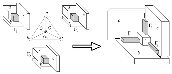
Figure 1: Illustration for the proof of Theorem 3.1.

First Proof: Let $a$, $b$, $c$ be the outer vertices of $G$. We construct a representation $\Gamma$ for $G$ where $b$ occupies the bottom side of $\Gamma$, $a$ occupies the back of $\Gamma-\{b\}$ and $c$ occupies the right side of $\Gamma-\{a,b\}$; see Fig. 1. Here for a set of vertices $S$, $\Gamma-S$ denotes the representation obtained from $\Gamma$ by deleting the boxes representing the vertices in $S$. The claim is trivial when $G$ is a triangle, so assume that $G$ has at least one internal vertex. Let $r$ be the root of the representation tree $T_{G}$ of $G$. Then $r$ is adjacent to $a$, $b$ and $c$ and thus defines three regions $G_{1}$, $G_{2}$ and $G_{3}$ inside the triangles $\Delta_{1}=abr$, $\Delta_{2}=bcr$ and $\Delta_{3}=car$, respectively (including the vertices of these triangles). By induction hypothesis $G_{i}$, $i=1,2,3$ has a proportional box-contact representation $\Gamma_{i}$ where the boxes for the three vertices in $\Delta_{i}$ occupy the bottom, back and right sides of $\Gamma_{i}$. Define $\Gamma^{\prime}_{i}=\Gamma_{i}-\Delta_{i}$. We now construct the desired representation for $G$. First take a box for $r$ with volume $w(r)$ and place it in a corner created by the intersection of three pairwise-touching boxes; see Fig. 1. For each $\Delta_{i}$, $i=1,2,3$, there is a corner $p_{i}$ formed by the intersection of the three boxes for $\Delta_{i}$. We now place $\Gamma^{\prime}_{i}$ (after possible scaling) in the corner $p_{i}$ so that it touches the boxes for the vertices in $\Delta_{i}$ by three planes. Note that this is always possible since we can choose the surface areas for $a$, $b$ and $c$ to be arbitrarily large and still realize their corresponding weights by appropriately changing the thickness in the third dimension. This construction requires only linear time, by keeping the scaling factor for each region in the representative tree $T_{G}$ at the vertex representing that region. Then the exact coordinates can be computed with a top-down traversal of $T_{G}$. ∎

Second Proof: Assume (after possible factoring) that for each vertex $v$ of $G$, the weight $w(v)$ is at least 1. Let $T_{G}$ be the representative tree of $G$. For any vertex $v$ of $T_{G}$, we denote by $U_{v}$, the set of the descendants of $v$ in $T_{G}$ including $v$. The predecessors of $v$ are the neighbors of $v$ in $G$ that are not in $U_{v}$. Clearly each vertex of $T_{G}$ has exactly three predecessors. We now define a parameter $W(v)$ for each vertex $v$ of $T_{G}$. Let $v_{1}$, $v_{2}$ and $v_{3}$ be the three children of $v$ in $T_{G}$ (where zero or more of these three children may be empty). Then $W(v)$ is defined as $\Pi_{i=1}^{3}[W(v_{i})+\sqrt[3]{w(v)}]$, where $U(v_{i})$ is taken as zero when $v_{i}$ is empty. We can compute the value of $W(v)$ for each vertex $v$ of $T_{G}$ by a linear-time bottom-up traversal of $T_{G}$. Once we have computed these values, we proceed on constructing the box-contact representation as follows.

Figure 2: Illustration for the second proof of Theorem 3.1.

Let $a$, $b$, $c$ be the three outer vertices of $G$ in the clockwise order and let $r$ be the root of $T_{G}$. We start by computing three boxes for $a$, $b$ and $c$ with the correct volume as illustrated in Fig. 2(a), so that the volume of the dotted box $R$ is $W(r)$. We will now construct a box representation of $U_{r}$ inside $R$ so that all the vertices in $U_{r}$ adjacent to an outer vertex is represented by a box with a face co-planar on the face of $R$ adjacent to box representing that outer vertex. We do this recursively by a top-down computation on $T_{G}$. Let $v$ be a vertex of $T_{G}$ with the three predecessors $u_{1}$, $u_{2}$ and $u_{3}$. Let $D(v)$ be a box with volume $W(v)$ and let $t_{1}$, $t_{2}$, $t_{3}$ be three faces of it with a common point. While traversing $v$, we compute a proportional box-contact representation of $U_{v}$ inside $D(v)$ where the vertices in $U_{v}$ adjacent to $u_{i}$ for some $i\in\{1,2,3\}$ is represented by a box with a face co-planar with $t_{i}$. Let $v_{1}$, $v_{2}$ and $v_{3}$ are the three children of $v$ in $T_{G}$ (where zero or more of these children may be empty). Also assume that $x_{1}$, $x_{2}$, $x_{3}$ are the length, width and height of $D(v)$, respectively and $p$ is the common point of $t_{1}$, $t_{2}$ and $t_{3}$. Then first compute a box $R(v)$ of volume $w(v)$ for $v$ with a corner at $p$ where $x^{\prime}_{1}$, $x^{\prime}_{2}$ and $x^{\prime}_{3}$ are the length, width and height of $R(v)$, such that $x^{\prime}_{i}=\frac{\sqrt[3]{w(v)}}{W(v_{1})+\sqrt[3]{w(v)}}$. These choices of $x^{\prime}_{i}$’s also creates three boxes $D(v_{i})$ with volume at least $W(v_{i})$, $i\in\{1,2,3\}$, as illustrated in Fig. 2(b). Finally we recursively compute the box representations for $U_{v_{i}}$ inside $D(v_{i})$ for $i\in\{1,2,3\}$ to complete the construction. ∎

Theorem 3.2

[5] Let $G$ be a plane 3-tree. Then a cube-contact representation of $G$ can be computed in linear time.

The proof of this claim also relies on the recursive decomposition of planar 3-trees.

4 Cube-Contacts for Nested Maximal Outerplanar Graphs

We prove the following main theorem in this section:

Theorem 4.1

Any nested maximal outerplanar graph has a proper contact representation with cubes.

We prove Theorem 4.1 by construction, starting with a representation for each piece of $G$, and combining the pieces to complete the representation for $G$.

Let $G$ be a nested maximal outerplanar graph. We first augment the graph $G$ by adding three mutually adjacent dummy vertices $\{A,B,C\}$ on the outerface and then triangulating the graph by adding dummy edges from these three vertices to the outer vertices of $G$ such that the graph remains planar; see Fig. 4(a). Call this graph the extended graph of $G$. For consistency, let the three dummy vertices have level $0$. The observation below follows from the definition of nested maximal outerplanar graphs.

Observation 1

Let $G$ be a nested-maximal planar graph and let $G^{\prime}$ be the extended graph of $G$. Then for each piece $P$ of $G$ at level $l$, there is a triangle of $(l-1)$-level vertices adjacent to the vertices of $P$ and no other $k$-level vertices with $k<l$ are adjacent to any vertex of $P$.

Given this observation, we use the following strategy to obtain a contact representation of $G$ with cubes. For each piece $P$ of $G$ at level $l$, let $A$, $B$ and $C$ be the three $(l-1)$-level vertices adjacent to $P$’s vertices. Let $P^{\prime}$ be the subgraph of $G$ induced vertices of $P$ as well as $A$, $B$ and $C$; call $P^{\prime}$ the extended piece of $G$ for $P$. We obtain a contact representation of $P^{\prime}$ with cubes and delete the three cubes for $A$, $B$ and $C$ to obtain the contact representation of $P$ with cubes. Finally, we combine the representations for the pieces to complete the desired representation of $G$.

Before we give more details on this algorithm, we have the following lemma, that we use in this section. Furthermore this result is also interesting by itself, since for any outerplanar graph $O$, where each face has at least one outer edge, Lemma 2 gives a contact representation of $O$ on the plane with squares such that the outer boundary of the representation is a rectangle.

Lemma 2

Let $G$ be planar graph with outerface $ABba$ and at least one internal vertex, such that $G-\{A,B\}$ is a maximal outerplanar graph. If there is no chord between any two neighbors of $A$ and no chord between any two neighbors of $B$, then $G$ has a contact representation $\Gamma$ in 2D where each inner vertex is represented by a square, the union of these squares forms a rectangle, and the four sides of these rectangles represent $A$, $B$, $b$ and $a$, respectively.

Proof

We prove this lemma by induction on the number of vertices in $G$. Denote the maximal outerplanar graph $H=G-\{A,B\}$; see Fig. 3(a). If $G$ contains only one internal vertex $v$, then we compute $\Gamma$ by representing $v$ by a square $R(v)$ of arbitrary size and representing $A$, $B$, $b$ and $a$ by the left, bottom, right and top sides of $R(v)$.

Figure 3: Illustration for the proof of Lemma 2.

We thus assume that $G$ has at least two internal vertices. Let $u$ be the unique common neighbor of $\{a,b\}$ in $H$. If $u$ is a neighbor of $A$, then $H-\{a\}$ is a maximal outerplanar graph. By induction hypothesis, $G-\{a\}$ has a contact representation $\Gamma^{\prime}$ where each internal vertex of $G-\{a\}$ is represented by a square and the left, bottom, right and top sides of $\Gamma^{\prime}$ represent $A$, $B$, $b$ and $u$. Then we compute $\Gamma$ from $\Gamma^{\prime}$ by adding a square $R(u)$ to represent $u$ such that $R(u)$ spans the entire width of $\Gamma^{\prime}$ and is placed on top of $\Gamma^{\prime}$; see Fig. 3(b). A similar construction can be used if $u$ is a neighbor of $B$; see Fig. 3(c). We thus compute a contact representation for $G$; see Fig. 3(d).

4.1 Cube-Contact Representation for Extended Pieces

Lemma 3

Let $P$ be a piece of $G$ at level $l$ and $P^{\prime}$ be the extended piece for $P$ with $(l-1)$-level vertices $A$, $B$, $C$. Then $P^{\prime}$ has a cube-contact representation.

Proof

Let $r$ be a common neighbor of $B$ and $C$; $s$ a common neighbor of $A$ and $C$; $t$ a common neighbor of $A$ and $B$. It is easy to find a contact representation of $P^{\prime}$ if $r$, $s$ and $t$ are the only vertices of $P$, so let $P$ have at least four vertices. The outer cycle of $P$ can be partitioned into three paths: $P_{a}$ is the path from $s$ to $t$, $P_{b}$ is the path from $r$ to $t$ and $P_{c}$ is the path from $r$ to $s$. Note that all vertices on the path $P_{a}$ ($P_{b}$, $P_{c}$) are adjacent to $A$ ($B$, $C$). A chord $(u,v)$ is a short chord if it is between two vertices on the same path from the set $\{P_{a},P_{b},P_{c}\}$. (Note that a chord between two vertices from the set $\{r,s,t\}$ is also a short chord.) We have the following two cases.

Case A: There is no short chord in $P$. In this case all the chords of $P$ are between two different paths. We consider the following two subcases.

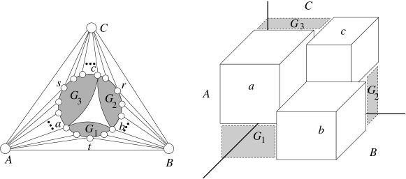
(a)                                                  (b)

Figure 4: Illustration for Case A1 in the proof of Lemma 3.

Case A1: There is no chord with one end-point in $\{r,s,t\}$. In this case, due to maximal-planarity there exist three vertices $a$, $b$ and $c$, adjacent to $A$, $B$, and $C$, respectively such that (i) $ab$ is the chord between vertices of $P_{a}$ and $P_{b}$ farthest away from $t$, (ii) $bc$ is the chord between vertices of $P_{b}$ and $P_{c}$ farthest away from $r$, and (iii) $ac$ is the chord between vertices of $P_{a}$ and $P_{c}$ farthest away from $s$; see Fig. 4(a). We can then find three interior-disjoint subgraphs of $P^{\prime}$ defined by three cycles of $P^{\prime}$: $G_{1}$ is the one induced by all vertices on or inside $ABba$; $G_{2}$ is induced by all vertices on or inside $BCcb$; and $G_{3}$ is induced by all vertices on or inside $ACca$. Each of these subgraphs has the common property that if we delete two vertices from the outerface (two vertices from the set $\{A,B,C\}$ in each subgraph), we get an outerplanar graph. From the representation with squares from the proof of Lemma 2, we find a contact representation of $G_{i}$, $i=1,2,3$ where each internal vertex of $G_{i}$ is represented by a cube and the union of all these cubes forms a rectangular box whose four sides realize the outer vertices. We use such a representation to obtain a contact representation of $P^{\prime}$ with cubes as follows.

We draw pairwise adjacent cubes (of arbitrary size) for $A$, $B$, $C$. We need to place the cubes for all the vertices of $P$ in the a corner defined by three faces of the cubes for $A$, $B$, $C$. Then we place three mutually touching cubes for $a$, $b$ and $c$, which touch the walls for $A$, $B$ and $C$, respectively; see Fig. 4(b). We also compute a contact representation of the internal vertices for each of the three graphs $G_{1}$, $G_{2}$ and $G_{3}$ with cubes using Lemma 2, so that the outer boundary for each of these representation forms a rectangular pipe. We adjust the sizes of the three cubes for $a$, $b$ and $c$ in such a way that the three highlighted rectangular pipes precisely fit these three representations (after some possible scaling). Note that this construction works even if one or more of the subgraphs $G_{1}$, $G_{2}$ and $G_{3}$ are empty. This completes the analysis of Case A1.

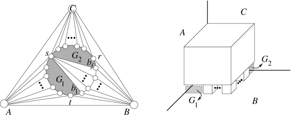
(a)                                                  (b)

Figure 5: Illustration for Case A2 in the proof of Lemma 3.

Case A2: There is at least one chord with one end-point in $\{r,s,t\}$. Due to planarity all such chords will have the same end-point in $\{r,s,t\}$. Suppose $s$ is this common end point for these chords; see Fig. 5(a). Let $b_{1}$ and $b_{f}$ be the first and last endpoints in the clockwise order of these chords around $s$. Then we can find two subgraphs $G_{1}$ and $G_{2}$ induced by the vertices on or inside two separating cycles $ABb_{1}s$ and $BCsb_{f}$. We find contact representations for the internal vertices of these two graphs $G_{1}$ and $G_{2}$ using Lemma 2 so that the outer-boundaries of these representation form rectangular pipes. We then obtain the desired contact representation for $P^{\prime}$, starting with the three mutually touching walls for $A$, $B$ and $C$ at right angles from each other, placing the cubes for $s$ and $b_{1}$, $\ldots$, $b_{f}$ as illustrated in Fig. 5(b), and fitting the representations for $G_{1}$ and $G_{2}$ (after some possible scaling) in the highlighted regions.

Case B: there are some shord chords in $P$. In this case, we find at most four subgraphs from $P^{\prime}$ as follows. At each path in $\{P_{a},P_{b},P_{c}\}$, we find the outermost chord, i.e., one that is not contained inside any other chords on the same path. Suppose these chords are $a_{1}a_{2}$, $b_{1}b_{2}$ and $c_{1}c_{2}$, on the three paths $P_{a}$, $P_{b}$, $P_{c}$, respectively. Then three of these subgraphs $G_{a}$, $G_{b}$ and $G_{c}$ are induced by the vertices on or inside the three triangles $Aa_{1}a_{2}$, $Bb_{1}b_{2}$ and $Cc_{1}c_{2}$. The fourth subgraph $P^{*}$ is obtained from $P^{\prime}$ by deleting all the inner vertices of the three graphs $G_{a}$, $G_{b}$ and $G_{c}$; see Fig. 6.

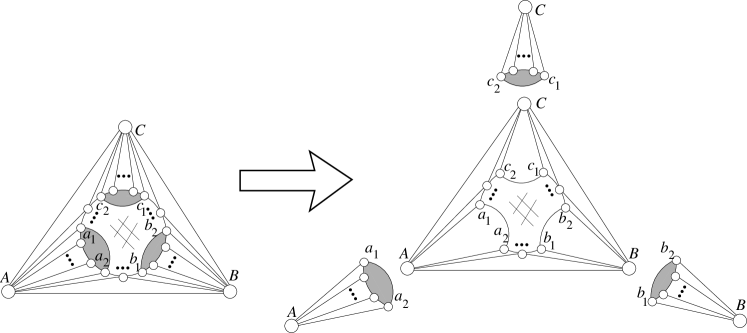
Figure 6: Removing chords with end-vertices in the same neighborhood.

A cube representation of $P^{*}$ can be found by the algorithm in Case A, as $P^{*}$ fits the condition that there is no chord between any two neighbors of the same vertex in $\{A,B,C\}$. Note that by moving the cubes in the representation by an arbitrarily small amount, we can make sure that for each triangle $xyz$ in $P^{*}$, the three cubes for $x$, $y$ and $z$ form a corner surrounded by three mutually touching walls at right angles to each other. Now observe that each of the three graphs $G_{a}$, $G_{b}$ and $G_{c}$ is a planar 3-tree; thus using the algorithm of either [5] or [10], we can place the internal vertices of these three graphs in their corresponding corners, thereby completing the representation.

4.2 Cube-Contact Representation for a Nested Maximal Outerplanar Graph

Proof of Theorem 4.1: Let $G$ be a nested maximal outerplanar graph. We build the contact representation of $G$ by a top-down traversal of the rooted tree $\mathcal{T}$ of the pieces of $G$. We start by creating a corner surrounded by three mutually touching walls at right angle to each other. Then whenever we traverse any vertex of $\mathcal{T}$, we realize the corresponding piece $P$ at level $l$ by obtaining a representation using Lemma 3 and placing this in the corner created by the three already-placed cubes for the three $(l-1)$-level vertices adjacent to $P$ (after possible scaling). ∎

5 Proportional Box-Contacts for Nested Outerplanar Graphs

In this section we prove the following main theorem.

Theorem 5.1

Let $G=(V,E)$ be a nested outerplanar graph and let $w:V\rightarrow\mathbb{R}^{+}$ be a weight function defining weights for the vertices of $G$. Then $G$ has a proportional contact representation with axis-aligned boxes with respect to $w$.

We construct a proportional representation for $G$ using a similar strategy as in the previous section: we traverse the construction tree $\mathcal{T}$ of $G$ and deal with each piece of $G$ separately. Each piece $P$ of $G$ is an outerplanar graph and hence one can easily construct a proportional box-contact representation for $P$ as follows. Any outerplanar graph $P$ has a contact representation with rectangles in the plane. In fact in [2], it was shown that $P$ has a contact representation with rectangles on the plane where the rectangles realize prespecified weights by their areas. Thus by giving unit heights to all rectangles we can obtain a proportional box-contact representation of $P$ for any given weight function. However if we construct proportional box-contact representation for each piece of $G$ in this way, it is not clear that we can combine them all to find a proportional contact representation of the whole graph $G$. Instead, we use this construction idea in Lemmas 4 and 5 to build two different proportional rectangle-contact representations for outerplanar graphs and we use them in the proof of Theorem 5.1.

Suppose $O$ is an outerplanar graph and $\Gamma$ is a contact representation of $O$ with rectangles in the plane. We say that a corner of a rectangle in $\Gamma$ is exposed if it is on the outer-boundary of $\Gamma$ and is not shared with any other rectangles.

Lemma 4

Let $O$ be a maximal outerplanar graph with a weight function $w$. Let $1$, $\ldots$, $n$ be the clockwise order of the vertices around the outer-cycle. Then a proportional rectangle-contact representation $\Gamma$ of $O$ for $w$ can be computed so that rectangle $R_{1}$ for $1$ is leftmost in $\Gamma$, rectangle $R_{n}$ for $n$ is bottommost in $\Gamma-R_{1}$, and the top-right corner for each rectangle is exposed in $\Gamma$.

Proof

We give an algorithm that recursively computes $\Gamma$. Constructing $\Gamma$ is easy when $G$ is a single edge $(1,n)$. We thus assume that $G$ has at least 3 vertices. Let $x$ be the (unique) third vertex on the inner face that is adjacent to $(1,n)$. Then graph $G$ can be split into two graphs at vertex $x$ and edge $(1,n)$: $G[1,x]$ consists of the graph induced by all vertices between $1$ and $x$ in clockwise order around the outer-cycle; while $G[x,n]$ consists of the graph induced by the vertices between $x$ and $n$.

Recursively draw $G[1,x]$ and remove the rectangles for $1$ and $x$ from it; call the result $\Gamma_{1}$. Again recursively draw $G[x,n]$ and remove $x$ and $n$ from it; call the result $\Gamma_{2}$. Now draw a rectangle $R_{x}$ for $x$ with area $w(x)$. Let $l_{x}$ and $h_{x}$ be the width and height of $R_{x}$, respectively. Then draw the rectangles $R_{1}$ and $R_{n}$ for $1$ and $n$ touching the left and the bottom sides of $R_{x}$, respectively with necessary areas. Select the widths and heights of these two rectangles such that the area $l_{x}(h_{1}-h_{n}-h_{x})$ can contain $\Gamma_{1}$ while the area $(w_{n}-w_{x})*h_{x}$ can contain $\Gamma_{2}$, where $l_{j}$ and $h_{j}$ denote the width and height of $R_{j}$, respectively for $j\in\{1,n\}$. Finally place $\Gamma_{1}$ (after possible scaling) touching the right side of $R_{1}$ and the top side of $R_{x}$ and place $\Gamma_{2}$ (after possible scaling) touching the right side of $R_{x}$ and the top side of $R_{n}$ to complete the drawing; see Fig. 8.

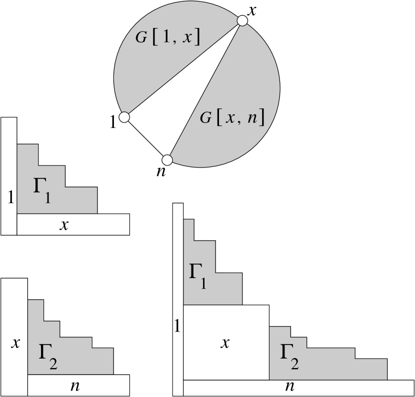
Figure 7: Illustration for the proof of Lemma 4.

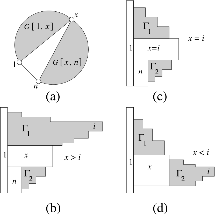
Figure 8: Illustration for the proof of Lemma 5.

Note that in the layout obtained above the top right corners of the rectangles for vertices $\{1,\ldots,n\}$ have increasing $x$-coordinates and decreasing $y$-coordinates. Thus we refer to them as Staircase layouts and to the algorithm as the Staircase Algorithm.

Lemma 5

Let $O$ be a maximal outerplanar graph with a weight function $w$. Let $1$, $\ldots$, $n$ be the clockwise order of the vertices around the outer-cycle. Then a proportional rectangle-contact representation $\Gamma$ of $O$ for $w$ can be computed so that rectangle $R_{1}$ for $1$ is leftmost in $\Gamma$, rectangle $R_{n}$ for $n$ is bottommost in $\Gamma-R_{1}$, and the top-right corners of all rectangles for vertices $\{1,\ldots,i\}$ and the bottom-right corners of all rectangles for vertices $\{i,\ldots,n\}$ are exposed in $\Gamma$.

Proof

We again compute $\Gamma$ recursively. Constructing $\Gamma$ is easy when $G$ is a single edge $(1,n)$. We thus assume that $G$ has at least 3 vertices. Let $x$ be the (unique) third vertex on the inner face that is adjacent to $(1,n)$. Define the two graphs $G[1,x]$ and $G[x,n]$ as in the proof of Lemma 4; see also Fig. 8(a).

If $x>i$, then recursively draw $G[1,x]$ and remove the rectangles for $1$ and $x$ from it; call the result $\Gamma_{1}$. Draw $G[x,n]$ using the Staircase Algorithm. Now draw three mutually touching rectangles $R_{1}$, $R_{x}$ and $R_{n}$ for $1$, $x$ and $n$, respectively with necessary areas such that the right side of $R_{1}$ touches both $R_{x}$ and $R_{n}$ and the right side of $R_{x}$ has greater $x$-coordinate than the right side of $R_{n}$; see Fig. 8(b). Finally place $\Gamma_{1}$ (after possible scaling) touching the right side of $R_{1}$ and the top side of $R_{x}$ such that the right side of the rectangle for $(x-1)$ extends past $R_{x}$. Also place $\Gamma_{2}$ (after $90^{\circ}$ clockwise rotation and possible scaling) touching the bottom side of $R_{x}$ and the right side of $R_{n}$ to complete the drawing (the width of $R_{x}$ can be chosen long enough so that $\Gamma_{2}$ can be contained between the bottom side of $R_{x}$ and the right side of $R_{n}$).

On the other hand if $x=i$ we follow almost the same procedure as in the previous paragraph. However, instead of the drawing of $G[1,x]$ recursively, we compute it by the Staircase Algorithm and then delete from it $1$ and $x$ to obtain $\Gamma_{1}$. We compute $\Gamma_{2}$ as in the previous section. We also draw $R_{1}$, $R_{x}$ and $R_{n}$ in the same way. Then we place $\Gamma_{1}$ (after possible scaling) touching the right side of $R_{1}$ and the top side of $R_{x}$ (again the width of $R_{x}$ is chosen long enough so that this can be done). We also place $\Gamma_{2}$ as the same manner as before to complete the drawing; see Fig. 8(c).

Finally if $x<i$, then we draw $G[1,x]$ by the Staircase Algorithm and delete from it $1$ and $x$ to obtain $\Gamma_{1}$. However, to compute $\Gamma_{2}$, we recursively draw $G[x,n]$ and delete $x$ and $n$ from it. We now draw $R_{1}$, $R_{x}$ and $R_{n}$ as before but this time the right side of $R_{n}$ should extend past $R_{x}$. We now place $\Gamma_{1}$ (after possible scaling) touching the right side of $R_{1}$ and the top side of $R_{x}$ (this is again possible for suitable choice of the height of $R_{1}$). Finally we complete the drawing by placing $\Gamma_{2}$ (after possible scaling) touching the right side of $R_{x}$ and the top side of $R_{n}$ so that the right side of the rectangle for $n-1$ extends past $R_{n}$; see Fig. 8(d).

Note that in the layout obtained above the top-right corners for vertices $\{1,\ldots,i\}$ and the bottom-right corners for vertices $\{i+1,\ldots,n\}$ form two staircases. Thus we refer to this as a Double-Staircase layout, to the algorithm as the Double-Staircase Algorithm, and to vertex $i$ as the pivot vertex.

Let $O$ be a maximal outerplanar graph and let $\Gamma$ be either a Staircase or a Double-Staircase layout. Then any triangle $\{p,q,r\}$ in $O$ is represented by three rectangles and the shared boundaries of these rectangles define a T-shape. The vertex whose two shared boundaries are collinear in the T-shape is called the pole of the triangle $\{p,q,r\}$.

Proof of Theorem 5.1. Let $\mathcal{T}$ be the construction tree for $G$. We compute a representation for $G$ by a top-down traversal of $\mathcal{T}$, constructing the representation for each piece as we traverse it. Let $P$ be a piece of $G$ at the $l$-th level. If $P$ is the root of $\mathcal{T}$, then we use the Staircase Algorithm to find a contact representation of $P$ with rectangles in the plane and then we give necessary heights to these rectangles to obtain a proportional contact representation of $P$ with boxes. Otherwise, the vertices of $P$ are adjacent to exactly three $(l-1)$-level vertices $A$, $B$, $C$ that form a triangle in the parent piece of $P$. Since $A$, $B$, $C$ belong to the parent piece of $P$, their boxes have already been drawn when we start to draw $P$. To find a correct representation of $G$, we need that the boxes for the vertices in $P$ have correct adjacencies with the boxes for $A$, $B$, and $C$; hence we assume a fixed structure for such a triangle. We maintain the following invariant:

Let $\{p,q,r\}$ be three vertices in a piece $P$ of $G$ forming a triangle. Then in the proportional contact representation of $P$, the boxes for $p$, $q$, $r$ are drawn in such a way that (i) the projection of the mutually shared boundaries for these boxes in the $xy$-plane forms a T-shape, (ii) the highest faces (faces with largest $z$-coordinate) of the three rectangles have different $z$ coordinates and the highest face of the pole-vertex of the triangle has the smallest $z$-coordinate.

Note that by choosing the areas of the rectangles in the Staircase layout, we can maintain this invariant for the parent piece by appropriately adjusting the heights of the boxes(e.g., incrementally increasing heights for the vertices in the recursive Staircase Algorithm).

We now describe the construction of a proportional box-contact representation of $P$ with the correct adjacencies for $A$, $B$ and $C$. By the invariant the projection of the shared boundaries for $\{A,B,C\}$ forms a T-shape in the $xy$-plane. Without loss of generality assume that $A$ is the pole of the triangle and the highest faces of $B$, $C$ and $A$ are in this order according to decreasing $z$-coordinates. Also assume that $P$ is a maximal outerplanar graph; we later argue that this assumption is not necessary.

Let $ab$ be a common neighbor of $A$ and $B$; $bc$ a common neighbor of $B$ and $C$; $ca$ a common neighbor of $C$ and $A$. Then the outer cycle of $P$ can be partitioned into three paths: $P_{a}$ is the path from $ca$ to $ab$, $P_{b}$ is the path from $ab$ to $bc$ and $P_{c}$ is the path from $bc$ to $ca$. All the vertices on the path $P_{a}$ ($P_{b}$, $P_{c}$, respectively) are adjacent to $A$ ($B$, $C$, respectively). We first assume that there is no chord in $P$ between $ca$ and a vertex on path $P_{a}$. We consider the following two cases.

Case 1: No vertex of $P$ is adjacent to all of $\{A,B,C\}$. We label the vertices of $P$ in the clockwise order starting from $ca=1$ and ending at $n$, where $n$ is the number of vertices in $P$. Let $i$ and $j$ be the indices of vertices $bc$ and $ab$, respectively. Let $x$ be the index of the vertex that is the (unique) third vertex of the inner face of $P$ containing the edge $(1,n)$. Define the two graphs $G[1,x]$ and $G[x,n]$ as in the proof of Lemma 4. We first find a proportional contact representation of $P$ for $w$ restricted to the vertices of $P$ using rectangles in the plane, then we give necessary heights to this rectangles. Draw $G[x,n]$ using the Staircase Algorithm and delete the rectangles for $x$ and $n$ to obtain $\Gamma_{2}$. Draw rectangles $R_{x}$ and $R_{n}$ for $x$ and $n$, respectively, so that the bottom side of $R_{x}$ touches the top side of $R_{n}$, the left sides for both the rectangles have the same $x$-coordinate and and the right side of $R_{n}$ extends past $R_{x}$. Now place $\Gamma_{2}$ (after possible scaling) touching the right side of $R_{x}$ and the top side of $R_{n}$ (this is possible since we can make the width of $R_{n}$ sufficiently long); see Fig. 9. Place the rectangle $R_{1}$ for $1$ touching the left sides of $R_{x}$ and $R_{n}$ such that its bottom side is aligned with $R_{n}$ and its top side is aligned with the top side of the rectangle for $j$. To complete the rest of the drawing, we have the following two subcases:

Case 1a: $x\leq i$. We draw $G[1,x]$ using the Staircase Algorithm and delete from it the rectangles for $1$ and $x$ to obtain $\Gamma_{1}$. We finally place $\Gamma_{1}$ (after $90^{\circ}$ counterclockwise rotation and possible scaling) touching the top side of $R_{1}$ and left side of $R_{x}$ (this is possible by choosing a sufficiently large height for $R_{x}$); see Fig. 9(a).

Case 1b: $x>i$. We draw $G[1,x]$ using the Double-Staircase Algorithm where $i$ is the pivot vertex. From this drawing, we delete the rectangles for $1$ and $x$ to obtain $\Gamma_{1}$. Finally place $\Gamma_{1}$ (after $90^{\circ}$ counterclockwise rotation and possible scaling) touching the top side of $R_{1}$ and left side of $R_{x}$ such that the topside of the rectangle for $(x-1)$ goes past the top side of $R_{x}$; see Fig. 9(b).

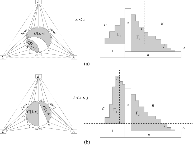
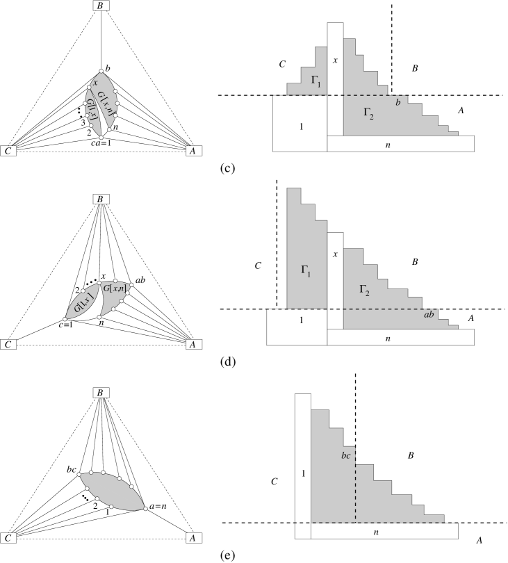
Figure 9: Illustration for Theorem 5.1. Construction of the representation for a piece $P$ of $G$, when (a)–(b) no vertex of $P$ is adjacent to all of $\{A,B,C\}$, and (c)–(e) a vertex of $P$ is adjacent to all of $\{A,B,C\}$.

So far we used the function $w$ to assign areas for the rectangles and obtained proportional box-contact representation of $P$ from the rectangles by assigning unit heights. However, by changing the areas for the rectangles, we can obtain different heights for the boxes. We will use this property to maintain adjacencies with $\{A,B,C\}$, as well as to maintain the invariant. Specifically, once we get the box representation of $P$, we scale it by increasing the heights for the boxes, so that when we place it at the corner created by the T-shape for $\{A,B,C\}$ it will not intersect the representation for any of its sibling pieces in $\mathcal{T}$. Consider the point $p$ which is the intersection of the lines containing the right side of the rectangle for $i$ and the top side of the rectangle for $j$. We place $\Gamma$ such that the point $p$ superimposes on the corner for the T-shape in the projection on the $xy$-plane. Since the highest faces of $B$, $C$ and $A$ are in this order according to $z$-coordinate, the adjacencies of the vertices in $P$ with $\{A,B,C\}$ are correct. By appropriately choosing the areas for the rectangles, we ensure that all the boxes for the vertices of $P$ have their highest faces above that of $B$ and that the invariant is maintained.

Case 2: A vertex of $P$ is adjacent to all of $\{A,B,C\}$. In this case at least one of $\{A,B,C\}$ has only one neighbor in $P$. Assume first that a vertex $b$ ($=ab=bc$) of $P$ is adjacent to all of $\{A,B,C\}$ and this is the only neighbor of $B$; see Fig. 9(c). Then we follow the steps for Case 1a with $b=j$ (and some vertex between $x$ and $b$ as $i$). But when we finally place this representation of $P$ on the corner for the T-shape of $\{A,B,C\}$ we find the point $p$ to superimpose on this corner as follows. The point $p$ is on the line containing the top side of the rectangle for $b$ and has $x$-coordinate between the right sides of the rectangles for $b$ and $(b-1)$.

If a vertex $c$ ($=bc=ca$) is adjacent to all of $\{A,B,C\}$ and is the only neighbor of $C$ in $P$, then we follow the steps of Case 1b with $i=2$ and $j=ab$; see Fig. 9(d). We find the point $p$ to superimpose on the corner for the T-shape of $\{A,B,C\}$ as follows. The point $p$ is on the line containing the top side of the rectangle for $j=ab$ and has $x$-coordinate between the left sides of the rectangles for $1$ and $2$.

If a vertex $a$ ($=ab=ca$) is adjacent to all of $\{A,B,C\}$ and is the only neighbor of $A$ in $P$, then we number the vertices of $P$ in the clockwise order starting from the clockwise neighbor of $a$ and ending at $a=n$; see Fig. 9(e). We use the Staircase Algorithm to find a representation of $P$ with rectangles and give necessary heights to obtain a representation with boxes. On the corner for the T-shape of $\{A,B,C\}$, we superimpose the intersection point for the lines containing the top side of the rectangle of $n$ and the right side of the rectangle for $bc$.

Finally, we consider the case when there is a chord between $ca$ and another vertex on the path $P_{a}$. Take the innermost such chord and let its other end-vertex be $t$. Then consider the two subgraphs $P_{1}$ and $P_{2}$ induced by all the vertices outside the chord and inside the chord (along with the two vertices $ca$ and $t$). $P_{1}$ does not contain any chord from $ca$; thus we use the algorithm above to obtain a representation of $P_{1}$; denote this by $\Gamma^{\prime}$. In this representation $ca$ and $t$ will play the roles of $1$ and $n$, respectively. Each vertex of $P_{2}$ is adjacent to $A$ and we find a proportional contact representation of $P_{2}$ and attach it with $\Gamma^{\prime}$ as follows. We use the Staircase Algorithm to find a proportional contact representation of $P_{2}$ with rectangles in the plane and delete the rectangles for $ca$ and $t$ from it to obtain $\Gamma^{\prime\prime}$. In $\Gamma^{\prime}$, we change the height of the rectangle $R_{1}$ for $ca=1$ to increase its area so that its bottom side extends past the bottom side of the rectangle $R_{n}$ for $t=n$. Then we place $\Gamma^{\prime\prime}$ (after reflecting with respect to the $x$-axis and possible scaling) touching the right side of $R_{1}$ and the bottom side of $R_{n}$. Since the Staircase Algorithm can accommodate any given area for the layout, we can change the heights of the boxes for the vertices in $P_{2}$ to maintain the invariant.

Thus with the top-down traversal of $\mathcal{T}$, we obtain a proportional contact representation for $O$. We assumed that each piece of $O$ is maximal outerplanar. However in the contact representation, for each edge $(u,v)$, either a face of the box $R_{u}$ for $u$ is adjacent to the box $R_{v}$ for $v$ and no other box; or a face of $R_{v}$ is adjacent to $R_{u}$ and no other box. In both cases the adjacency between these two coxes can be removed without affecting any other adjacency. Thus this algorithm holds for any nested outerplanar graph $O$. ∎

6 Conclusions and Future Work

We proved that nested maximal outerplanar graphs have cube-contact representations and nested outerplanar graphs have proportional box-contact representations. These classes of graphs are special cases of $k$-outerplanar graphs, and the set of $k$-outerplanar graphs for all $k>0$ is equivalent to the class of all planar graphs. Even though our approach might generalize to large classes, cube-contact representations and proportional box-contact representations are still open for general planar graphs.

Acknowledgments: We thank Therese Biedl, Steve Chaplick, Stefan Felsner, and Torsten Ueckerdt for discussions about this problem.

References

- [1] Alam, M.J., Kobourov, S.G., Liotta, G., Pupyrev, S., Veeramoni, S.: 3D proportional contact representations of graphs. In: Bourbakis, N.G., Tsihrintzis, G.A., Virvou, M. (eds.) Information, Intelligence, Systems and Applications. pp. 27–32. IEEE (2014)
- [2] Alam, M.J., Biedl, T.C., Felsner, S., Gerasch, A., Kaufmann, M., Kobourov, S.G.: Linear-time algorithms for hole-free rectilinear proportional contact graph representations. Algorithmica 67(1), 3–22 (2013)
- [3] Biedl, T.C., Velázquez, L.E.R.: Drawing planar 3-trees with given face areas. Computational Geometry: Theory and Applications 46(3), 276–285 (2013)
- [4] Biedl, T.C., Velázquez, L.E.R.: Orthogonal cartograms with at most 12 corners per face. Computational Geometry: Theory and Applications 47(2), 282–294 (2014)
- [5] Bremner, D., Evans, W.S., Frati, F., Heyer, L.J., Kobourov, S.G., Lenhart, W.J., Liotta, G., Rappaport, D., Whitesides, S.: On representing graphs by touching cuboids. In: Didimo, W., Patrignani, M. (eds.) Graph Drawing. LNCS, vol. 7704, pp. 187–198. Springer (2012)
- [6] Buchsbaum, A.L., Gansner, E.R., Procopiuc, C.M., Venkatasubramanian, S.: Rectangular layouts and contact graphs. ACM Transactions on Algorithms 4(1) (2008)
- [7] Duncan, C.A., Gansner, E.R., Hu, Y.F., Kaufmann, M., Kobourov, S.G.: Optimal polygonal representation of planar graphs. Algorithmica 63(3), 672–691 (2012)
- [8] Eppstein, D., Mumford, E., Speckmann, B., Verbeek, K.: Area-universal and constrained rectangular layouts. SIAM Journal on Computing 41(3), 537–564 (2012)
- [9] Evans, W., Felsner, S., Kaufmann, M., Kobourov, S., Mondal, D., Nishat, R., Verbeek, K.: Table cartograms. In: Bodlaender, H.L., Italiano, G.F. (eds.) European Symposium on Algorithms. LNCS, vol. 8125, pp. 421–432. Springer (2013)
- [10] Felsner, S., Francis, M.C.: Contact representations of planar graphs with cubes. In: Hurtado, F., van Kreveld, M.J. (eds.) Symposium on Computational Geometry. pp. 315–320 (2011)
- [11] de Fraysseix, H., de Mendez, P.O.: Regular orientations, arboricity, and augmentation. In: Graph Drawing. LNCS, vol. 894, pp. 111–118. Springer (1995)
- [12] Fusy, É.: Transversal structures on triangulations: A combinatorial study and straight-line drawings. Discrete Mathematics 309(7), 1870–1894 (2009)
- [13] Koebe, P.: Kontaktprobleme der konformen Abbildung. Berichte über die Verhandlungen der Sächsischen Akad. der Wissenschaften zu Leipzig. Math.-Phys. Klasse 88, 141–164 (1936)
- [14] Kozminski, K., Kinnen, E.: Rectangular duals of planar graphs. Networks 15(2), 145–157 (1985)
- [15] van Kreveld, M.J., Speckmann, B.: On rectangular cartograms. Computational Geometry 37(3), 175–187 (2007)
- [16] Mondal, D., Nishat, R.I., Rahman, M.S., Alam, M.J.: Minimum-area drawings of plane 3-trees. Journal of Graph Algorithms and Applications 15(2), 177–204 (2011)
- [17] Thomassen, C.: Interval representations of planar graphs. Journal of Combinatorial Theory, Series B 40(1), 9–20 (1988)
- [18] Ungar, P.: On diagrams representing maps. Journal of the London Mathematical Society 28, 336–342 (1953)
- [19] Yeap, K.H., Sarrafzadeh, M.: Floor-planning by graph dualization: 2-concave rectilinear modules. SIAM Journal on Computing 22, 500–526 (1993)