A complex hyperbolic Riley slice

Abstract

We study subgroups of ${\rm PU}(2,1)$ generated by two non-commuting unipotent maps $A$ and $B$ whose product $AB$ is also unipotent. We call $\mathcal{U}$ the set of conjugacy classes of such groups. We provide a set of coordinates on $\mathcal{U}$ that make it homeomorphic to $\mathbb{R}^{2}$ . By considering the action on complex hyperbolic space $\mathbf{H}^{2}_{\mathbb{C}}$ of groups in $\mathcal{U}$, we describe a two dimensional disc ${\mathcal{Z}}$ in $\mathcal{U}$ that parametrises a family of discrete groups. As a corollary, we give a proof of a conjecture of Schwartz for $(3,3,\infty)$-triangle groups. We also consider a particular group on the boundary of the disc ${\mathcal{Z}}$ where the commutator $[A,B]$ is also unipotent. We show that the boundary of the quotient orbifold associated to the latter group gives a spherical CR uniformisation of the Whitehead link complement.

AMS classification 51M10, 32M15, 22E40

1 Introduction

1.1 Context and motivation

The framework of this article is the study of the deformations of a discrete subgroup $\Gamma$ of a Lie group $H$ in a Lie group $G$ containing $H$. This question has been addressed in many different contexts. A classical example is the one where $\Gamma$ is a Fuchsian group, $H={\rm PSL}(2,\mathbb{R})$ and $G={\rm PSL}(2,\mathbb{C})$. When $\Gamma$ is discrete, such deformations are called quasi-Fuchsian. We will be interested in the case where $\Gamma$ is a discrete subgroup of $H={\rm SO}(2,1)$ and $G$ is the group ${\rm SU}(2,1)$ (or their natural projectivisations over $\mathbb{R}$ and $\mathbb{C}$ respectively). The geometrical motivation is very similar: In the classical case mentioned above, ${\rm PSL}(2,\mathbb{C})$ is the orientation preserving isometry group of hyperbolic 3-space ${\bf H}^{3}$ and a Fuchsian group preserves a totally geodesic hyperbolic plane ${\bf H}^{2}$ in ${\bf H}^{3}$. In our case $G={\rm SU}(2,1)$ is (a triple cover of) the holomorphic isometry group of complex hyperbolic 2-space $\mathbf{H}^{2}_{\mathbb{C}}$, and the subgroup $H={\rm SO}(2,1)$ preserves a totally geodesic Lagrangian plane isometric to ${\bf H}^{2}$. A discrete subgroup $\Gamma$ of ${\rm SO}(2,1)$ is called $\mathbb{R}$-Fuchsian. A second example of this construction is where $G$ is again ${\rm SU}(2,1)$ but now $H={\rm S}\bigl{(}{\rm U}(1)\times{\rm U}(1,1)\bigr{)}$. In this case $H$ preserves a totally geodesic complex line in $\mathbf{H}^{2}_{\mathbb{C}}$. A discrete subgroup of $H$ is called $\mathbb{C}$-Fuchsian. Deformations of either $\mathbb{R}$-Fuchsian or $\mathbb{C}$-Fuchsian groups in ${\rm SU}(2,1)$ are called complex hyperbolic quasi-Fuchsian. See [25] for a survey of this topic.

The title of this article refers to the so-called Riley slice of Schottky space (see [19] or [1]). Riley considered the space of conjugacy classes of subgroups of ${\rm PSL}(2,\mathbb{C})$ generated by two non-commuting parabolic maps. This space may be identified with $\mathbb{C}-\{0\}$ under the map that associates the parameter $\rho\in\mathbb{C}-\{0\}$ with the conjugacy class of the group $\Gamma_{\rho}$, where

$$\Gamma_{\rho}=\left\langle\left[\begin{matrix}1&1\\ 0&1\end{matrix}\right],\ \left[\begin{matrix}1&0\\ \rho&1\end{matrix}\right]\right\rangle.$$

Riley was interested in the set of those parameters $\rho$ for which $\Gamma_{\rho}$ is discrete. He was particularly interested in the (closed) set where $\Gamma_{\rho}$ is discrete and free, which is now called the Riley slice of Schottky space [19]. This work has been taken up more recently by Akiyoshi, Sakuma, Wada and Yamashita. In their book [1] they illustrate one of Riley’s original computer pictures, Figure 0.2a, and their version of this picture, Figure 0.2b. Riley’s main method was to construct the Ford domain for $\Gamma_{\rho}$. The different combinatorial patterns that arise in this Ford domain correspond to the differently coloured regions in these figures from [1]. Riley was also interested in groups $\Gamma_{\rho}$ that are discrete but not free. In particular, he showed that when $\rho$ is a complex sixth root of unity then the quotient of hyperbolic 3-space by $\Gamma_{\rho}$ is the figure-eight knot complement.

1.2 Main definitions and discreteness result

The direct analogue of the Riley slice in complex hyperbolic plane would be the set of conjugacy classes of groups generated by two non-commuting, unipotent parabolic elements $A$ and $B$ of ${\rm SU}(2,1)$. (Note that in contrast to to ${\rm PSL}(2,\mathbb{C})$, there exist parabolic elements in ${\rm SU}(2,1)$ that are not unipotent. In fact, there is a 1-parameter family of parabolic conjugacy classes, see for instance Chapter 6 of [15].) This choice would give a four dimensional parameter space, and we require additionally that $AB$ is unipotent; making the dimension drop to $2$. Specifically, we define

$${\mathcal{U}=\Bigl{\{}(A,B)\in{\rm SU}(2,1)^{2}\ :\ A,\,B,\,AB\,\hbox{ all unipotent and }AB\neq BA\Bigr{\}}}/{SU(2,1)}.$$ (1)

Following Riley, we are interested in the (closed) subset of ${\mathcal{U}}$ where the group $\langle A,B\rangle$ is discrete and free and our main method for studying this set is to construct the Ford domain for its action on complex hyperbolic space $\mathbf{H}^{2}_{\mathbb{C}}$. We shall also indicate various other interesting discrete groups in ${\mathcal{U}}$ but these will not be our main focus.

In Section 3.1, we will parametrise $\mathcal{U}$ so that it becomes the open square $(-\pi/2,\pi/2)^{2}$. The parameters we use will be the Cartan angular invariants $\alpha_{1}$ and $\alpha_{2}$ of the triples of (parabolic) fixed points of $(A,AB,B)$ and $(A,AB,BA)$ respectively (see Section 2.6 for the definitions). Note that the invariants $\alpha_{1}$ and $\alpha_{2}$ are defined to lie in the closed interval $[-\pi/2,\pi/2]$. Our assumption that $A$ and $B$ don’t commute implies that neither $\alpha_{1}$ nor $\alpha_{2}$ can equal $\pm\pi/2$ (see Section 3.1).

When $\alpha_{1}$ and $\alpha_{2}$ are both zero, that is at the origin of the square, the group $\langle A,B\rangle$ is ${\mathbb{R}}$-Fuchsian. The quotient of the Lagrangian plane preserved by $\langle A,B\rangle$ is a hyperbolic three times punctured sphere where the three (homotopy classes of) peripheral elements are represented by (the conjugacy classes of) $A$, $B$ and $AB$. The space $\mathcal{U}$ can thus be thought of as the slice of the ${\rm SU}(2,1)$-representation variety of the three times punctured sphere group defined by the conditions that the peripheral loops are mapped to unipotent isometries.

We can now state our main discreteness result.

Theorem 1.1.

Suppose that $\Gamma=\langle A,B\rangle$ is the group associated to parameters $(\alpha_{1},\alpha_{2})$ satisfying $\mathcal{D}\bigl{(}4\cos^{2}(\alpha_{1}),4\cos^{2}(\alpha_{2})\bigr{)}>0$, where $\mathcal{D}$ is the polynomial given by

$$\mathcal{D}(x,y)=x^{3}y^{3}-9x^{2}y^{2}-27xy^{2}+81xy-27x-27.$$

Then $\Gamma$ is discrete and isomorphic to the free group $F_{2}$. This region is $\mathcal{Z}$ in Figure 1.

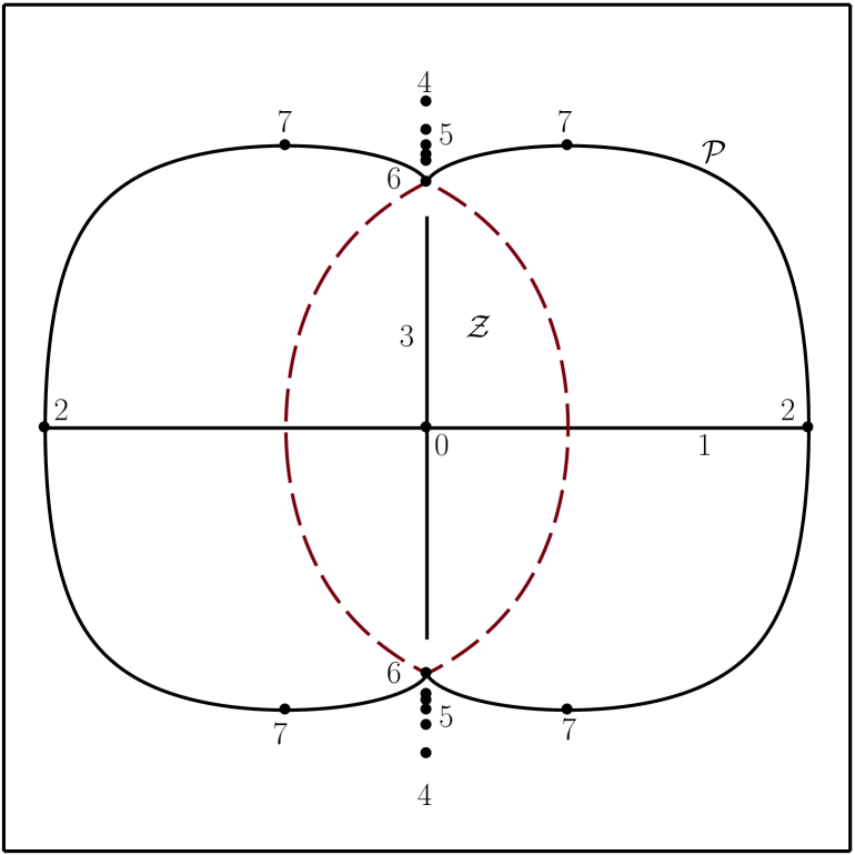
0 $\mathbb{R}$-Fuchsian representation of the $3$-punctured sphere group. 1 The horizontal segment marked $1$ corresponds to even word subgroups of ideal triangle groups, see [16, 30, 31, 33]. 2 Last ideal triangle group, contained with index three in a group uniformising the Whitehead link complement obtained by Schwartz, see [30, 31, 33]. 3 The vertical segment marked $3$ corresponds to bending groups that have been proved to be discrete in [37]. 4 $(3,3,4)$-group uniformising the figure eight knot complement. Obtained by Deraux and Falbel in [8]. 5 $(3,3,n)$-groups, proved to be discrete by in [26]. On this picture $4\leqslant n\leqslant 8$. 6 Uniformisation of the Whitehead link complement we obtain in this work. 7 Subgroup of the Eisenstein-Picard Lattice, see [14].

Figure 1: The parameter space for $\mathcal{U}$. The exterior curve $\mathcal{P}$ corresponds to classes of groups for which $[A,B]$ is parabolic. The central dashed curve bounds the region $\mathcal{Z}$ where we prove discreteness. The labels correspond to various special values of the parameters. Points with the same labels are obtained from one another by symmetries about the coordinate axes. The results of Section 3.3 imply that they correspond to groups conjugate in Isom($\mathbf{H}^{2}_{\mathbb{C}}$).

Note that at the centre of the square, we have $\mathcal{D}(4,4)=1225$ for the ${\mathbb{R}}$-Fuchsian representation. The region ${\mathcal{Z}}$ where ${\mathcal{D}}>0$ consists of groups $\Gamma$ whose Ford domain has the simplest possible combinatorial structure. It is the analogue of the outermost region in the two figures from Akiyoshi, Sakuma, Wada and Yamashita [1] mentioned above.

1.3 Decompositions and triangle groups

We will prove in Proposition 3.2 that all pairs $(A,B)$ in $\mathcal{U}$ admit a (unique) decomposition of the form

$$A=ST\mbox{ and }B=TS,$$ (2)

where $S$ and $T$ are order three regular elliptic elements (see Section 2.2). In turn, the group generated by $A$ and $B$ has index three in the one generated by $S$ and $T$. When either $\alpha_{1}=0$ or $\alpha_{2}=0$ there is a further decomposition making $\langle A,B\rangle$ a subgroup of a triangle group.

Deformations of triangle groups in ${\rm PU}(2,1)$ have been considered in many places, among which ([16, 28, 32, 26]). A complex hyperbolic $(p,q,r)$-triangle is one generated by three complex involutions about (complex) lines with pairwise angles $\pi/p$, $\pi/q$, and $\pi/r$ where $p$, $q$ and $r$ are integers or $\infty$ (when one of them is $\infty$ the corresponding angle is $0$). Groups generated by complex reflections of higher order are also interesting, see [22] for example, but we do not consider them here. For a given triple $(p,q,r)$ with $\min\{p,q,r\}\geqslant 3$ the deformation space of the $(p,q,r)$-triangle group is one dimensional, and can be thought of as the deformation space of the $\mathbb{R}$-Fuchsian triangle group. In [32], Schwartz develops a series of conjectures about which points in this space yield discrete and faithful representations of the triangle group. For a given triple $(p,q,r)$, Conjecture 5.1 of [32] states that a complex hyperbolic $(p,q,r)$-triangle group is a discrete and faithful representation of the Fuchsian one if and only if the words $I_{i}I_{j}I_{k}$ and $I_{i}I_{j}I_{k}I_{j}$ (with $i,j,k$ pairwise distinct) are non-elliptic. Moreover, depending on $p$, $q$ and $r$ he predicts which of these words one should choose.

We now explain the relationship between triangle groups and groups on the axes of our parameter space ${\mathcal{U}}$. First consider groups with $\alpha_{2}=0$. Let $I_{1}$, $I_{2}$ and $I_{3}$ be the involutions fixing the complex lines spanned by the fixed points of $(A,\,B)$, of $(A,\,AB)$ and of $(B,\,AB)$ respectively. If $\alpha_{2}=0$ then $A$ and $B$ may be decomposed as $A=I_{2}I_{1}$ and $B=I_{1}I_{3}$, and also $\langle A,B\rangle$ has index 2 in $\langle I_{1},I_{2},I_{3}\rangle$ (Proposition 3.6). Since $I_{2}I_{1}=A$, $I_{1}I_{3}=B$ and $I_{2}I_{3}=AB$ are all unipotent, we see that $\langle I_{1},I_{2},I_{3}\rangle$ is a complex hyperbolic ideal triangle group, as studied by Goldman and Parker [16] and Schwartz [30, 31, 33]. Their results gave a complete characterisation of when such a group is discrete. (Our Cartan invariant $\alpha_{1}$ is the same as the Cartan invariant $\mathbb{A}$ used in these papers.)

Theorem 1.2 (Goldman, Parker [16], Schwartz [31, 33]).

Let $I_{1}$, $I_{2}$, $I_{3}$ be complex involutions fixing distinct, pairwise asymptotic complex lines. Let $\mathbb{A}$ be the Cartan invariant of the fixed points of $I_{1}I_{2}$, $I_{2}I_{3}$ and $I_{3}I_{1}$.

1. The group $\langle I_{1},I_{2},I_{3}\rangle$ is a discrete and faithful representation of an $(\infty,\infty,\infty)$-triangle group if and only if $I_{1}I_{2}I_{3}$ is non-elliptic. This happens when $|\mathbb{A}|\leq\arccos\sqrt{3/128}$.

2. When $I_{1}I_{2}I_{3}$ is elliptic the group is not discrete. In this case $\arccos\sqrt{3/128}<|\mathbb{A}|<\pi/2$.

When $\alpha_{1}=0$ we get an analogous result. In this case, it is the order three maps $S$ and $T$ from (2) which decompose into products of complex involutions. Namely, if $\alpha_{1}=0$, there exist three involutions $I_{1}$, $I_{2}$, $I_{3}$, each fixing a complex line, so that $S=I_{2}I_{1}$ and $T=I_{1}I_{3}$ have order 3 and $ST=A=I_{2}I_{3}$ is unipotent (Proposition 3.6). Furthermore, writing $B=TS=I_{1}I_{3}I_{2}I_{1}$ we have $[A,B]=(ST^{-1})^{3}=(I_{2}I_{1}I_{3}I_{1})^{3}$. A corollary of Theorem 1.1 is a statement analogous to Theorem 1.2 for $(3,3,\infty)$-triangle groups, proving a special case of Conjecture 5.1 of Schwartz [32]. Compare with the proof of this conjecture for $(3,3,n)$-triangle groups given by Parker, Wang and Xie in [26].

Theorem 1.3.

Let $I_{1}$, $I_{2}$ and $I_{3}$ be complex involutions fixing distinct complex lines and so that $S=I_{2}I_{1}$ and $T=I_{1}I_{3}$ have order three and $A=ST=I_{2}I_{3}$ is unipotent. Let $\mathbb{A}$ be the Cartan invariant of the fixed points of $A$, $SAS^{-1}$ and $S^{-1}AS$. The group $\langle I_{1},I_{2},I_{3}\rangle$ is a discrete and faithful representation of the $(3,3,\infty)$-triangle group if and only if $I_{2}I_{1}I_{3}I_{1}=ST^{-1}$ is non-elliptic. This happens when $|\mathbb{A}|\leq\arccos\sqrt{3/8}$.

Theorem 1.3 follows directly from Theorem 1.1 by restricting it to the case where $(\alpha_{1},\alpha_{2})=(0,\mathbb{A})$. These groups are a special case of those studied by Will in [37] from a different point of view. There, using bending he proved that these groups are discrete as long as $|\mathbb{A}|=|\alpha_{2}|\leq\pi/4$. The gap between the vertical segment in Figure 1 and the curve where $[A,B]$ is parabolic illustrates the non-optimality of the result of [37].

1.4 Spherical CR uniformisations of the Whitehead link complement

The quotient of $\mathbf{H}^{2}_{\mathbb{C}}$ by an $\mathbb{R}$ or $\mathbb{C}$-Fuchsian punctured surface group is a disc bundle over the surface. If the surface is non-compact, this bundle is trivial. Its boundary at infinity is a circle bundle over the surface. Such three-manifolds appearing on the boundary at infinity of quotients of $\mathbf{H}^{2}_{\mathbb{C}}$ are naturally equipped with a spherical CR structure, which is the analogue of the flat conformal structure in the real hyperbolic case. These structures are examples of $(X,G)$-structure, where $X=S^{3}=\partial\mathbf{H}^{2}_{\mathbb{C}}$ and $G={\rm PU}(2,1)$. To any such structure on a three manifold $M$ are associated a holonomy representation $\rho:\pi_{1}(M)\longrightarrow{\rm PU}(2,1)$ and a developing map $D=\widetilde{M}\longrightarrow X$. This motivates the study of representations of fundamental groups of hyperbolic three manifolds in ${\rm PU}(2,1)$ and ${\rm PGL}(3,\mathbb{C})$ initiated by Falbel in [11], and continued in [13, 12] (see also [18]). Among ${\rm PU}(2,1)$-representations, uniformisations (see Definition 1.3 in [7]) are of special interest. There, the manifold at infinity is the quotient of the discontinuity region by the group action.

For parameter values in the open region $\mathcal{Z}$, the manifold at infinity of $\mathbf{H}^{2}_{\mathbb{C}}/\langle S,T\rangle$ is a Seifert fibre space over a $(3,3,\infty)$-orbifold. This is obviously true in the case where $\alpha_{1}=\alpha_{2}=0$ (the central point on Figure 1). Indeed, for these values the group $\langle S,T\rangle$ preserves $\mathbf{H}^{2}_{\mathbb{R}}$ (it is $\mathbb{R}$-Fuchsian) and the fibres correspond to boundaries of real planes orthogonal to $\mathbf{H}^{2}_{\mathbb{R}}$. As the combinatorics of our fundamental domain remains unchanged in $\mathcal{Z}$, the topology of the quotient is constant in $\mathcal{Z}$.

Things become interesting if we deform the group in such a way that a loop on the surface is represented by a parabolic map: the topology of the manifold at infinity can change. A hyperbolic manifold arising in this way was first constructed by Schwartz:

Theorem 1.4 (Schwartz [30]).

Let $I_{1}$, $I_{2}$ and $I_{3}$ be as in Theorem 1.2. Let $\mathbb{A}$ be the Cartan invariant of the fixed points of $I_{1}I_{2}$, $I_{2}I_{3}$ and $I_{3}I_{1}$ and let $S$ be the regular elliptic map cyclically permuting these points. When $I_{1}I_{2}I_{3}$ is parabolic the quotient of $\mathbf{H}^{2}_{\mathbb{C}}$ by the group $\langle I_{1}I_{2},S\rangle$ is a complex hyperbolic orbifold with isolated singularities whose boundary at infinity is a spherical CR uniformisation of the Whitehead link complement. These groups have Cartan invariant $\mathbb{A}=\pm\arccos\sqrt{3/128}$,

Schwartz’s example provides a uniformisation of the Whitehead link complement. More recently, Deraux and Falbel described a uniformisation of the complement of the figure eight knot in [8]. In [6], Deraux proved that this uniformisation was flexible: he described a one parameter deformation of the uniformisation described in [8], each group in the deformation being a uniformisation of the figure eight knot complement.

Our second main result concerns the $(3,3,\infty)$ triangles group from Theorem 1.3, and it states that when $I_{2}I_{1}I_{3}I_{1}$ is parabolic the associated groups give a uniformisation of the Whitehead link complement which is different from Schwartz’s one. Indeed in our case the cusps of the Whitehead link complement both have unipotent holonomy. In Schwartz’s case, one of them is unipotent whereas the other is screw-parabolic. The representation of the Whitehead link group we consider here was identified from a different point of view by Falbel, Koseleff and Rouillier in their census of ${\rm PGL}(3,{\mathbb{C}})$ representations of knot and link complement groups, see page 254 of [13].

Theorem 1.5.

Let $I_{1}$, $I_{2}$ and $I_{3}$ be as in Theorem 1.3 and define $S=I_{2}I_{1}$ and $A=I_{2}I_{3}$. Let $\mathbb{A}$ be the Cartan invariant of the fixed points of $A$, $SAS^{-1}$ and $S^{-1}AS$. When $I_{2}I_{1}I_{3}I_{1}$ is parabolic the quotient of $\mathbf{H}^{2}_{\mathbb{C}}$ by $\langle A,S\rangle$ is a complex hyperbolic orbifold with isolated singularities whose boundary is a spherical CR uniformisation of the Whitehead link complement. These groups have Cartan invariant $\mathbb{A}=\pm\arccos\sqrt{3/8}$.

Schwartz’s uniformisation of the Whitehead link complement corresponds to each of the endpoints of the horizontal segment, marked 2 in Figure 1, and our uniformisation corresponds to each of the points on the vertical axis, marked 6 in that figure.

It should be noted that the image of the holonomy representation of our uniformisation of the Whitehead link complement is the group generated by $S$ and $T$, which is isomorphic to ${\mathbb{Z}}_{3}*{\mathbb{Z}}_{3}$. We note in Proposition 3.3 that the fundamental group of the Whitehead link complement surjects onto ${\mathbb{Z}}_{3}*{\mathbb{Z}}_{3}$. Furthermore the group ${\mathbb{Z}}_{3}*{\mathbb{Z}}_{3}$ is the fundamental group of the (double) Dehn filling of the Whitehead link complement with slope $-3$ at each cusp in the standard marking (the same as in SnapPy). This Dehn filling is non-hyperbolic, as can be easily verified using the software SnapPy [5] (it also follows from Theorem 1.3. in [20]). This fact should be compared with Deraux’s remark in [7] that all known examples of non-compact finite volume hyperbolic manifold admitting a spherical CR uniformisation also admit an exceptional Dehn filling which is a Seifert fibre space over a $(p,q,r)$-orbifold with $p,q,r,\geqslant 3$.

1.5 Ideas for proofs.

Proof of Theorem 1.1.

The rough idea of this proof is to construct fundamental domains for the groups corresponding to parameters in the region $\mathcal{Z}$. To this end, we construct their Ford domains, which can be thought of as a fundamental domain for a coset decomposition of the group with respect to a parabolic element (here, this element is $A=ST$). The Ford domain is invariant by the subgroup generated by $A$ and we obtain a fundamental domain for the group by intersecting the Ford domain with a fundamental domain for the subgroup generated by $A$. The sides of the Ford domain are built out of pieces of isometric spheres of various group elements (see Sections 6 and 4) This method is classical, and is described in the case of the Poincaré disc in Section 9.6 of Beardon [2].

We thus have to consider a 2-parameter family of such polyhedra, and the polynomial $\mathcal{D}$ controls the combinatorial complexity of the Ford domain within our parameter space for $\mathcal{U}$ in the following sense. The null-locus of $\mathcal{D}$ is depicted on Figure 1 as a dashed curve, which bounds the region $\mathcal{Z}$. In the interior of this curve, the combinatorics of our domain is constant, and stays the same as it is for the $\mathbb{R}$-Fuchsian group. On the boundary of $\mathcal{Z}$ the isometric spheres of the elements $S$, $S^{-1}$ and $T$ have a common point. More precisely, the isometric spheres of $S^{-1}$ and $T$ intersect for all values of $\alpha_{1}$ and $\alpha_{2}$, but inside $\mathcal{Z}$ their intersection is contained in one of the two connected components of the complement of the isometric sphere of $S$ in $\mathbf{H}^{2}_{\mathbb{C}}$. When one reaches the boundary curve of $\mathcal{Z}$, one of their intersection points lies on the isometric sphere of $S$.

We believe that it should be possible to mimic Riley’s approach and to construct regions in our parameter space where the Ford domain is more complicated. However, as with Riley’s work, this may only be reasonable via computer experiments.

Proof of Theorem 1.5.

The groups where $[A,B]=(I_{2}I_{1}I_{3}I_{1})^{3}$ is parabolic are the focus of Section 6 and Theorem 1.5 will follow from Theorem 6.4. In order to prove this result, we analyse in details our fundamental domain, and show that it gives the classical description of the Whitehead link complement from an ideal octahedron equipped with face identifications. The Whitehead link is depicted in Figure 2. We refer to Section 10.3 of Ratcliffe [29] and Section 3.3 of Thurston [35] for classical information about the topology of the Whitehead link complement and its hyperbolic structure.

1.6 Further remarks

Other discrete groups appearing in $\mathcal{U}$.

As well as the ideal triangle groups and bending groups discussed above, there are some other previously studied discrete groups in this family. We give them in $(\alpha_{1},\alpha_{2})$ coordinates and illustrate them in Figure 1.

1. The groups corresponding to $\alpha_{1}=0$ and $\alpha_{2}=\pm\arccos\sqrt{1/8}$ have been studied in great detail by Deraux and Falbel who proved that they give a spherical CR uniformisation of the figure-eight knot complement [8]. This illustrates the fact that there is no statement for Theorem 1.3 analogous to the second part of Theorem 1.2: the group from [8] is contained in a discrete (non-faithful) $(3,3,\infty)$ triangle groups where $I_{2}I_{1}I_{3}I_{1}$ is elliptic.

2. The groups with parameters $\alpha_{1}=0$ and for which $ST^{-1}$ has order $n$ correspond to the $(3,3,n)$ triangle groups studied by Parker, Wang and Xie in [26]. The corresponding value of $\alpha_{2}$ is given by $\alpha_{2}=\pm\arccos\sqrt{(4\cos^{2}(\pi/n)-1)/8}$.

3. The groups where $\alpha_{1}=\pm\pi/6$ and $\alpha_{2}=\pm\pi/3$ are discrete, since they are subgroups of the Eisenstein-Picard lattice ${\rm PU}(2,1;{\mathbb{Z}}[\omega])$, where $\omega$ is a cube root of unity. That lattice has been studied by Falbel and Parker in [14].

Comparison with the classical Riley slice.

There is, conjecturally, one extremely significant difference between the classical Riley slice and our complex hyperbolic version. The boundary of the classical Riley slice is not a smooth curve and has a dense set of points where particular group elements are parabolic (see for instance the beautiful picture in the introduction of [19]). On the other hand, we believe that in the complex hyperbolic case, discreteness is completely controlled by the commutator $[A,B]$, or equivalently $ST^{-1}$, as is true for the two cases where $\alpha_{1}=0$ or $\alpha_{2}=0$ described above. If this is true, then the boundary of the set of (classes of) discrete and faithful representations in ${\rm SU}(2,1)$ of the three punctured sphere group with unipotent peripheral holonomy is piecewise smooth, and it is given by the simple closed curve ${\mathcal{P}}$ in Figure 1. This curve provides a one parameter family of (conjecturally discrete) representations that connects Schwartz’s uniformisation of the Whitehead link complement to ours. We believe that all these representations give uniformisations of the Whitehead link complement as well, but we are not able to prove this with our techniques. What seems to happen is that if one deforms our uniformisation by following the curve $\mathcal{P}$, the number of isometric spheres contributing to the boundary at infinity of the Ford domain becomes too large to be understood using our techniques. Possibly, this is because deformations of fundamental domains with tangencies between bisectors is complicated. This should be compared to Deraux’s construction [6] of deformations of the figure-eight knot complement mentioned above. There, he had to use a different domain to the one in [8], which also has tangencies between the bisectors.

1.7 Organisation of the article.

This article is organised as follows. In Section 2 we present the necessary background facts on complex hyperbolic space and its isometries. In Section 3, we describe coordinates on the space of (conjugacy classes) of group generated by two unipotent isometries with unipotent product. Section 4 is devoted to the description of the isometric spheres that bound our fundamental domains. We state and apply the Poincaré polyhedron theorem in Section 5. In Section 6, we focus on the specific case where the commutator becomes parabolic, and prove that the corresponding manifold at infinity is homeomorphic to the complement of the Whitehead link. In Section 7, we give the technical proofs which we have omitted for readability in the earlier sections.

1.8 Acknowledgements

The authors would like to thank Miguel Acosta, Martin Deraux, Elisha Falbel and Antonin Guilloux for numerous interesting discussions. The second author thanks Craig Hodgson, Neil Hoffman and Chris Leininger for kindly answering his naïve questions. This research was financially supported by ANR SGT and an LMS Scheme 2 grant. The research took place during visits of both authors to Les Diablerets, Durham, Grenoble, Hunan University, ICTP and Luminy, and we would like to thank all these institutions for hospitality. We are very grateful to the referee for their careful report and many helpful suggestions for improvement of the paper. The second author had the pleasure to share a very useful discussion with Lucien Guillou on a sunny June afternoon in Grenoble. Lucien has since passed away, and we remember him with affection.

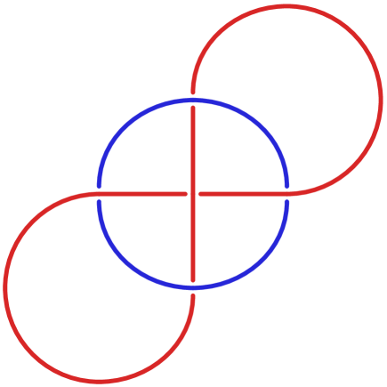
Figure 2: The Whitehead link

2 Preliminary material

Throughout we will work in the complex hyperbolic plane using a projective model and will therefore pass from projective objects to lifts of them. Our convention is that the same letter will be used to denote a point in $\mathbb{C}P^{2}$ and a lift of it to $\mathbb{C}^{3}$ with a bold font for the lift. As an example, each time $p$ is a point of $\mathbf{H}^{2}_{\mathbb{C}}$, ${\bf p}$ will be a lift of $p$ to $\mathbb{C}^{3}$.

2.1 The complex hyperbolic plane

The standard reference for complex hyperbolic space is Goldman’s book [15]. A lot of information can also be found in Chen and Greenberg’s paper [3], see also the survey articles [25, 38].

Let $H$ be the following matrix

$$H=\begin{bmatrix}0&0&1\\ 0&1&0\\ 1&0&0\end{bmatrix}.$$

The Hermitian product on $\mathbb{C}^{3}$ associated to $H$ is given by $\langle{\bf x},{\bf y}\rangle={\bf y}^{*}H{\bf x}$. The corresponding Hermitian form has signature $(2,1)$, and we denote by $V_{-}$ (respectively $V_{0}$ and $V_{+}$) the associated negative (respectively null and positive) cones in $\mathbb{C}^{3}$.

Definition 1.

The complex hyperbolic plane $\mathbf{H}^{2}_{\mathbb{C}}$ is the image of $V_{-}$ in $\mathbb{C}P^{2}$ by projectivisation and its boundary $\partial\mathbf{H}^{2}_{\mathbb{C}}$ is the image of $V_{0}$ in $\mathbb{C}P^{2}$. The complex hyperbolic plane is endowed with the Bergman metric

$$ds^{2}=\frac{-4}{\langle{\bf z},{\bf z}\rangle^{2}}{\rm det}\left(\begin{matrix}\langle{\bf z},{\bf z}\rangle&\langle d{\bf z},{\bf z}\rangle\\ \langle{\bf z},d{\bf z}\rangle&\langle d{\bf z},d{\bf z}\rangle\end{matrix}\right).$$

The Bergman metric is equivalent to the Bergman distance function $\rho$ defined by

$$\cosh^{2}{\left(\dfrac{\rho(m,n)}{2}\right)}=\dfrac{\langle{\bf m},{\bf n}\rangle\langle{\bf n},{\bf m}\rangle}{\langle{\bf m},{\bf m}\rangle\langle{\bf n},{\bf n}\rangle},$$

where ${\bf m}$ and ${\bf n}$ are lifts of $m$ and $n$ to $\mathbb{C}^{3}$.

Let ${\bf z}=[z_{1},\,z_{2},\,z_{3}]^{T}$ be a (column) vector in $\mathbb{C}^{3}-\{{\bf 0}\}$. Then ${\bf z}\in V_{-}$ (respectively $V_{0}$) if and only if $2{\rm Re}(z_{1}\overline{z}_{3})+|z_{2}|^{2}<0$ (respectively $=0$). Vectors in $V_{0}$ with $z_{3}=0$ must have $z_{2}=0$ as well. Such a vector is unique up to scalar multiplication. We call such its projectivisation the point at infinity $q_{\infty}\in\partial\mathbf{H}^{2}_{\mathbb{C}}$. If $z_{3}\neq 0$ then we can use inhomogeneous coordinates with $z_{3}=1$. Writing $\langle{\bf z},{\bf z}\rangle=-2u$ we give $\mathbf{H}^{2}_{\mathbb{C}}\cup\partial\mathbf{H}^{2}_{\mathbb{C}}-\{q_{\infty}\}$ horospherical coordinates $(z,t,u)\in\mathbb{C}\times\mathbb{R}\times\mathbb{R}_{\geq 0}$ defined as follows. A point $q\in\mathbf{H}^{2}_{\mathbb{C}}\cup\partial\mathbf{H}^{2}_{\mathbb{C}}$ with horospherical coordinates $(z,t,u)$ is represented by the following vector, which we call its standard lift.

$${\bf q}=\begin{bmatrix}-|z|^{2}-u+it\\ z\sqrt{2}\\ 1\end{bmatrix}\mbox{ if }q\neq q_{\infty},\quad{\bf q}_{\infty}=\begin{bmatrix}1\\ 0\\ 0\end{bmatrix}\mbox{ if }q=q_{\infty}.$$ (3)

Points of $\partial\mathbf{H}^{2}_{\mathbb{C}}-\{q_{\infty}\}$ have $u=0$ and we will abbreviate $(z,t,0)$ to $[z,t]$.

Horospherical coordinates give a model of complex hyperbolic space analogous to the upper half plane model of the hyperbolic plane. The Cygan metric $d_{\rm Cyg}$ on $\partial\mathbf{H}^{2}_{\mathbb{C}}-\{q_{\infty}\}$ plays the role of the Euclidean metric on the upper half plane. It is defined by the distance function:

$$d_{\rm Cyg}(p,q)=\bigl{|}\langle{\bf p},{\bf q}\rangle\bigr{|}^{1/2}=\Bigl{|}|z-w|^{2}+i\bigl{(}t-s+{\rm Im}(z\overline{w})\bigr{)}\Bigr{|}^{1/2}$$ (4)

where $p$ and $q$ have horospherical coordinates $[z,t]$ and $[w,s]$. We may extend this metric to points $p$ and $q$ in $\mathbf{H}^{2}_{\mathbb{C}}$ with horospherical coordinates $(z,t,u)$ and $(w,s,v)$ by writing

$$d_{\rm Cyg}(p,q)=\Bigl{|}|z-w|^{2}+|u-v|+i\bigl{(}t-s+{\rm Im}(z\overline{w})\bigr{)}\Bigr{|}^{1/2}$$

If (at least) one of $p$ and $q$ lies in $\partial\mathbf{H}^{2}_{\mathbb{C}}$ then we still have the formula $d_{\rm Cyg}(p,q)=\bigl{|}\langle{\bf p},{\bf q}\rangle\bigr{|}^{1/2}$.

2.2 Isometries

Since the Bergman metric and distance function are both given solely in terms of the Hermitian form, any unitary matrix preserving this form is an isometry. Similarly, complex conjugation of points in $\mathbb{C}^{3}$ leaves both the metric and the distance function unchanged. Hence, complex conjugation is also an isometry.

Define ${\rm U}(2,1)$ to be the group of unitary matrices preserving the Hermitian form and ${\rm PU}(2,1)$ to be the projective unitary group obtained by identifying non-zero scalar multiples of matrices in ${\rm U}(2,1)$. We also consider the subgroup ${\rm SU}(2,1)$ of matrices in ${\rm U}(2,1)$ with determinant $1$.

Proposition 2.1.

Every Bergman isometry of $\mathbf{H}^{2}_{\mathbb{C}}$ is either holomorphic or anti-holomorphic. The group of holomorphic isometries is ${\rm PU}(2,1)$, acting by projective transformations. Every antiholomorphic isometry is complex conjugation followed by an element of ${\rm PU}(2,1)$.

Elements of ${\rm SU}(2,1)$ fall into three types, according to the number and type of the fixed points of the corresponding isometry. Namely, an isometry is loxodromic (respectively parabolic) if it has exactly two fixed points (respectively exactly one fixed point) on $\partial\mathbf{H}^{2}_{\mathbb{C}}$. It is called elliptic when it has (at least) one fixed point inside $\mathbf{H}^{2}_{\mathbb{C}}$. An elliptic element $A\in{\rm SU}(2,1)$ is called regular elliptic whenever it has three distinct eigenvalues, and special elliptic if it has a repeated eigenvalue. The following criterion distinguishes the different isometry types.

Proposition 2.2 (Theorem 6.2.4 of Goldman [15]).

Let $\mathcal{F}$ be the polynomial given by $\mathcal{F}(z)=|z|^{4}-8\mbox{\rm Re}\,(z^{3})+18|z|^{2}-27$, and $A$ be a non identity matrix in ${\rm SU}(2,1)$. Then

1. $A$ is loxodromic if and only if $\mathcal{F}(\mbox{\rm tr}A)>0$,

2. $A$ is regular elliptic if and only if $\mathcal{F}(\mbox{\rm tr}A)<0$,

3. if $\mathcal{F}(\mbox{\rm tr}A)=0$, then $A$ is either parabolic or special elliptic.

We will be especially interested in elements of ${\rm SU}(2,1)$ with trace $0$ and those with trace $3$.

Lemma 2.3 (Section 7.1.3 of Goldman [15]).

1. A matrix $A$ in ${\rm SU}(2,1)$ is regular elliptic of order three if and only if its trace is equal to zero.

2. Let $(p,q,r)$ be three pairwise distinct points in $\partial\mathbf{H}^{2}_{\mathbb{C}}$, not contained in a common complex line. Then there exists a unique order three regular elliptic isometry $E$ so that $E(p)=q$ and $E(q)=r$.

Suppose that $T\in{\rm SU}(2,1)$ has trace equal to $3$. Then all $T$ eigenvalues of $T$ equal $1$, that is $T$ is unipotent. If $T$ is diagonalisable then it must be the identity; if it is non-diagonalisable then it must fix a point of $\partial\mathbf{H}^{2}_{\mathbb{C}}$. Conjugating within ${\rm SU}(2,1)$ if necessary, we may assume that $T$ fixes $q_{\infty}$. This implies that $T$ is upper triangular with each diagonal element equal to $1$.

Lemma 2.4 (Section 4.2 of Goldman [15]).

Suppose that $[w,s]\in\partial\mathbf{H}^{2}_{\mathbb{C}}-\{q_{\infty}\}$. Then there is a unique $T_{[w,s]}\in{\rm SU}(2,1)$ taking the point $[0,0]\in\partial\mathbf{H}^{2}_{\mathbb{C}}$ to $[w,s]$. As a matrix this map is:

$$T_{[w,s]}=\begin{bmatrix}1&-\overline{w}\sqrt{2}&-|w|^{2}+is\\ 0&1&w\sqrt{2}\\ 0&0&1\end{bmatrix}.$$ (5)

Moreover, composition of such elements gives $\partial\mathbf{H}^{2}_{\mathbb{C}}-\{q_{\infty}\}$ the structure of the Heisenberg group

$$[w,s]\cdot[z,t]=\bigl{[}w+z,s+t-2{\rm Im}(z\overline{w})\bigr{]}$$

and $T_{[w,s]}$ acts as left Heisenberg translation on $\partial\mathbf{H}^{2}_{\mathbb{C}}-\{q_{\infty}\}$.

The action of $T_{[w,s]}$ on horospherical coordinates is:

$$T_{[w,s]}:(z,t,u)\longmapsto\bigl{(}w+z,s+t-2{\rm Im}(z\overline{w}),u\bigr{)}.$$

An important observation is that this is an affine map, namely a translation and shear.

We can restate Lemma 2.4 in an invariant way. This result is actually true for any parabolic conjugacy class, as a special case of Proposition 3.1 in [23].

Proposition 2.5.

Let $(p_{1},p_{2},p_{3})$ be a triple of pairwise distinct points in $\partial\mathbf{H}^{2}_{\mathbb{C}}$. Then there is a unique unipotent element of ${\rm PU}(2,1)$ fixing $p_{1}$ and taking $p_{2}$ to $p_{3}$.

Proof.

We can choose $A\in{\rm SU}(2,1)$ taking $p_{1}$ to $q_{\infty}$ and $p_{2}$ to $[0,0]$. The result then follows from Lemma 2.4. ∎

2.3 Totally geodesic subspaces.

Maximal totally geodesic subspaces of $\mathbf{H}^{2}_{\mathbb{C}}$ have real dimension 2, and they fall in two types. Complex lines are intersections with $\mathbf{H}^{2}_{\mathbb{C}}$ of projective lines in $\mathbb{C}P^{2}$. By Hermitian duality, any complex line $L$ is polar to a point in $\mathbb{C}P^{2}$ that is outside the closure of $\mathbf{H}^{2}_{\mathbb{C}}$. Any lift of this point is called a polar vector to $L$. Any two distinct points $p$ and $q$ in the closure of $\mathbf{H}^{2}_{\mathbb{C}}$ belong to a unique complex line, and a vector polar to this line is given by ${\bf p}\boxtimes{\bf q}=H\overline{{\bf p}\wedge{\bf q}}$. This can be verified directly using $\langle{\bf x},{\bf y}\rangle={\bf y}^{*}H{\bf x}$ and the fact that here, $H^{2}=1$. A more general description of cross products in Hermitian vector spaces can be found in Section 2.2.7. of Chapter 2 of Goldman [15].

The other type of maximal totally geodesic subspace is a Lagrangian plane. Lagrangian planes are ${\rm PU}(2,1)$ images of the set of real points $\mathbf{H}^{2}_{\mathbb{R}}\subset\mathbf{H}^{2}_{\mathbb{C}}$. In particular, real planes are fixed points sets of antiholomorphic isometric involutions (sometimes called real symmetries). The symmetry fixing $\mathbf{H}^{2}_{\mathbb{R}}$ is complex conjugation. In turn, the symmetry about any other Lagrangian plane $M\cdot\mathbf{H}^{2}_{\mathbb{R}}$, where $M\in{\rm SU}(2,1)$, is given by ${\bf z}\longmapsto M\overline{M^{-1}}\,\overline{\bf z}=M\overline{\bigl{(}M^{-1}{\bf z}\bigr{)}}$. Note that the matrix $N=M\overline{M^{-1}}$ satisfies $N\overline{N}=Id$: this reflects the fact that real symmetries are involutions. We refer the reader to Chapter 3 and 4 of Goldman [15].

2.4 Isometric spheres

Definition 2.

For any $B\in{\rm SU}(2,1)$ that does not fix $q_{\infty}$, the isometric sphere of $B$ (denoted $\mathcal{I}(B)$) is defined to be

$$\mathcal{I}(B)=\Bigl{\{}p\in\mathbf{H}^{2}_{\mathbb{C}}\cup\partial\mathbf{H}^{2}_{\mathbb{C}}\ :\ \bigl{|}\langle{\bf p},{\bf q}_{\infty}\rangle\bigr{|}=\bigl{|}\langle{\bf p},B^{-1}({\bf q}_{\infty})\rangle\bigr{|}=\bigl{|}\langle B({\bf p}),{\bf q}_{\infty}\rangle\bigr{|}\Bigr{\}}$$ (6)

where ${\bf p}$ is the standard lift of $p\in\mathbf{H}^{2}_{\mathbb{C}}\cup\partial\mathbf{H}^{2}_{\mathbb{C}}$ given in (3).

The interior of $\mathcal{I}(B)$ is the component of its complement in $\mathbf{H}^{2}_{\mathbb{C}}\cup\partial\mathbf{H}^{2}_{\mathbb{C}}$ that do not contain $q_{\infty}$, namely,

$$\Bigl{\{}p\in\mathbf{H}^{2}_{\mathbb{C}}\cup\partial\mathbf{H}^{2}_{\mathbb{C}}\ :\ \bigl{|}\langle{\bf p},{\bf q}_{\infty}\rangle\bigr{|}>\bigl{|}\langle{\bf p},B^{-1}({\bf q}_{\infty})\rangle\bigr{|}\Bigr{\}}.$$

The exterior of $\mathcal{I}(B)$ is the component that contains the point at infinity $q_{\infty}$

Suppose $B$ is written as a matrix as

$$B=\left[\begin{matrix}a&b&c\\ d&e&f\\ g&h&j\end{matrix}\right].$$ (7)

Then $B^{-1}({\bf q}_{\infty})=\bigl{[}\overline{j},\,\overline{h},\,\overline{g}\bigr{]}^{T}$. Thus $B$ fixes $q_{\infty}$ if and only if $g=0$. If $B$ does not fix $q_{\infty}$ (that is $g\neq 0$) the horospherical coordinates of $B^{-1}(q_{\infty})$ are:

$$B^{-1}(q_{\infty})=\Bigl{[}\overline{h}/\bigl{(}\overline{g}\sqrt{2}\bigr{)},\,{\rm Im}\bigl{(}\overline{j}/\overline{g}\bigr{)}\Bigr{]}.$$

Lemma 2.6 (Section 5.4.5 of Goldman [15]).

Let $B\in{\rm PU}(2,1)$ be an isometry of $\mathbf{H}^{2}_{\mathbb{C}}$ not fixing $q_{\infty}$.

1. The transformation $B$ maps $\mathcal{I}(B)$ to $\mathcal{I}(B^{-1})$, and the interior of $\mathcal{I}(B)$ to the exterior of $\mathcal{I}(B^{-1})$.

2. For any $A\in{\rm PU}(2,1)$ fixing $q_{\infty}$ and such that the corresponding eigenvalue has unit modulus, we have $\mathcal{I}(B)=\mathcal{I}(AB)$.

Using the characterisation (4) of the Cygan metric in terms of the Hermitian form, the following lemma is obvious.

Lemma 2.7.

Suppose that $B\in{\rm SU}(2,1)$ written in the form (7) does not fix $q_{\infty}$. Then the isometric sphere $\mathcal{I}(B)$ is the Cygan sphere in $\mathbf{H}^{2}_{\mathbb{C}}\cup\partial\mathbf{H}^{2}_{\mathbb{C}}$ with centre $B^{-1}(q_{\infty})$ and radius $r_{A}=1/|g|^{1/2}$.

The importance of isometric spheres is that they form the boundary of the Ford polyhedron. This is the limit of Dirichlet polyhedra as the centre point approaches $\partial\mathbf{H}^{2}_{\mathbb{C}}$; see Section 9.3 of Goldman [15]. The Ford polyhedron $D$ for a discrete group $\Gamma$ is the intersection of the (closures of the) exteriors of all isometric spheres for elements of $\Gamma$ not fixing $q_{\infty}$. That is:

$$D_{\Gamma}=\Bigl{\{}p\in\mathbf{H}^{2}_{\mathbb{C}}\cup\partial\mathbf{H}^{2}_{\mathbb{C}}\ :\ \bigl{|}\langle{\bf p},{\bf q}_{\infty}\rangle\bigr{|}\geq\bigl{|}\langle{\bf p},B^{-1}{\bf q}_{\infty}\rangle\bigr{|}\hbox{ for all }B\in\Gamma\hbox{ with }B(q_{\infty})\neq q_{\infty}\Bigr{\}}.$$

Of course, just as for Dirichlet polyhedra, to construct the Ford polyhedron one must check infinitely many equalities. Therefore our method will be to guess the Ford polyhedron and check this using the Poincaré polyhedron theorem. When $q_{\infty}$ is either in the domain of discontinuity or is a parabolic fixed point, the Ford polyhedron is preserved by $\Gamma_{\infty}$, the stabiliser of $q_{\infty}$ in $\Gamma$. It is a fundamental polyhedron for the partition of $\Gamma$ into $\Gamma_{\infty}$-cosets. In order to obtain a fundamental domain for $\Gamma$, one must intersect the Ford domain with a fundamental domain for $\Gamma_{\infty}$.

2.5 Cygan spheres and geographical coordinates.

We now give some geometrical results about Cygan spheres. They are, in particular, applicable to isometric spheres. The Cygan sphere $\mathcal{S}_{[0,0]}(r)$ of radius $r>0$ with centre the origin $[0,0]$ is the (real) hypersurface of $\mathbf{H}^{2}_{\mathbb{C}}\cup\partial\mathbf{H}^{2}_{\mathbb{C}}$ described in horospherical coordinates by the equation

$$\mathcal{S}_{[0,0]}(r)=\Bigl{\{}(z,t,u)\ :\ \bigl{(}|z|^{2}+u\bigr{)}^{2}+t^{2}=r^{4}\Bigr{\}}.$$ (8)

From (8) we immediately see that when written in horospherical coordinates the interior of $\mathcal{S}_{[0,0]}(r)$ is convex. The Cygan sphere $\mathcal{S}_{[w,s]}(r)$ of radius $r$ with centre $[w,s]$ is the image of $\mathcal{S}_{[0,0]}(r)$ under the Heisenberg translation $T_{[w,s]}$. Since Heisenberg translations are affine maps in horospherical coordinates, we see that the interior of any Cygan sphere is convex. This immediately gives:

Proposition 2.8.

The intersection of two Cygan spheres is connected.

Cygan spheres are examples of bisectors (otherwise called spinal hypersurfaces) and their intersection is an example of what Goldman calls an intersection of covertical bisectors. Thus Proposition 2.8 is a restatement of Theorem 9.2.6 of [15]. There is a natural system of coordinates on bisectors in terms of totally geodesic subspaces, see Section 5.1 of [15]. In particular for Cygan spheres, these are defined as follows:

Definition 3.

Let ${\mathcal{S}}_{[0,0]}(r)$ be the Cygan sphere with centre the origin $[0,0]$ and radius $r>0$. The point $g(\alpha,\beta,w)$ of ${\mathcal{S}}_{[0,0]}(r)$ with geographical coordinates $(\alpha,\beta,w)$ is the point whose lift to $\mathbb{C}^{3}$ is:

$${\bf g}(\alpha,\beta,w)=\begin{bmatrix}-r^{2}e^{-i\alpha}\\ rwe^{i(-\alpha/2+\beta)}\\ 1\end{bmatrix},$$ (9)

where $\beta\in[0,\pi)$, $\alpha\in[-\pi/2,\pi/2]$ and $w\in[-\sqrt{2\cos(\alpha)},\sqrt{2\cos(\alpha)}]$,

Let ${\mathcal{S}}_{[z,t]}(r)$ be the Cygan sphere with centre $[z,t]$ and radius $r$. Then geographical coordinates on ${\mathcal{S}}_{[z,t]}(r)$ are obtained from the ones on ${\mathcal{S}}_{[0,0]}(r)$ by applying the Heisenberg translation $T_{[z,t]}$ to the vector (9).

We will only be interested in geographical coordinates on ${\mathcal{S}}_{[0,0]}(1)$, the unit Cygan sphere centred at the origin. Note that for the point $g(\alpha,\beta,w)$ of this sphere, $\langle g(\alpha,\beta,u),g(\alpha,\beta,u)\rangle=w^{2}-2\cos(\alpha)$. Therefore the horospherical coordinates of $g(\alpha,\beta,w)$ are:

$$\Bigl{(}we^{i(-\alpha/2+\beta)}/\sqrt{2},\ \sin(\alpha),\,\cos(\alpha)-w^{2}/2\Bigr{)}$$

In particular, the points of ${\mathcal{S}}_{[0,0]}(1)$ on $\partial\mathbf{H}^{2}_{\mathbb{C}}$ are those with $w=\pm\sqrt{2\cos(\alpha)}$.

The level sets of $\alpha$ and $\beta$ are totally geodesic subspaces of $\mathbf{H}^{2}_{\mathbb{C}}$; see Example 5.1.8 of Goldman [15].

Proposition 2.9.

Let ${\mathcal{S}}_{[w,s]}(r)$ be a Cygan sphere with geographical coordinates $(\alpha,\beta,w)$.

1. For each $\alpha_{0}\in(-\pi/2,\pi/2)$ the set of points $L_{\alpha_{0}}=\bigl{\{}g(\alpha,\beta,w)\in{\mathcal{S}}_{[w,s]}(r)\ :\ \alpha=\alpha_{0}\bigr{\}}$ is a complex line, called a slice of ${\mathcal{S}}_{[w,s]}(r)$.

2. For each $\beta_{0}\in[0,\pi)$ the set of points $R_{\beta_{0}}=\bigl{\{}g(\alpha,\beta,w)\in{\mathcal{S}}_{[w,s]}(r)\ :\ \beta=\beta_{0}\bigr{\}}$ is a Lagrangian plane, called a meridian of ${\mathcal{S}}_{[w,s]}(r)$.

3. The set of points with $w=0$ is the spine of ${\mathcal{S}}_{[w,s]}(r)$. It is a geodesic contained in every meridian.

Remark 1.

From (8), it is easy to see that projections of boundaries of Cygan spheres onto the $z$-factor are closed Euclidean discs in $\mathbb{C}$. This correspond to the vertical projection onto $\mathbb{C}$ in the Heisenberg group. This fact is often useful to prove that two Cygan spheres are disjoint.

2.6 Cartan’s angular invariant.

Élie Cartan defined an invariant of triples of pairwise distinct points $p_{1},\,p_{2},\,p_{3}$ in $\partial\mathbf{H}^{2}_{\mathbb{C}}$; see Section 7.1 of Goldman [15]. For any lifts ${\bf p}_{j}$ of $p_{j}$ to $\mathbb{C}^{3}$, this invariant is defined by $\mbox{arg}{\left(-\langle{\bf p}_{1},{\bf p}_{2}\rangle\langle{\bf p}_{2}{\bf p}_{3}\rangle\langle{\bf p}_{3},{\bf p}_{1}\rangle\right)}$, where the argument is chosen to lie in $(-\pi,\pi]$. We state here some important properties of $\mathbb{A}$.

Proposition 2.10.

[Sections 7.1.1 and 7.1.2 of [15]]

1. $-\pi/2\leq\mathbb{A}(p_{1},p_{2},p_{3})\leq\pi/2$ for any triple of pairwise distinct points $p_{1}$, $p_{2}$, $p_{3}$.

2. $\mathbb{A}(p_{1},p_{2},p_{3})=\pm\pi/2$ if and only if $p_{1}$, $p_{2}$, $p_{3}$ lie on the same complex line.

3. $\mathbb{A}(p_{1},p_{2},p_{3})=0$ if and only if $p_{1}$, $p_{2}$, $p_{3}$ lie on the same Lagrangian plane.

4. Two triples $p_{1}$, $p_{2}$, $p_{3}$ and $q_{1}$, $q_{2}$, $q_{3}$ have $\mathbb{A}(p_{1},p_{2},p_{3})=\mathbb{A}(q_{1},q_{2},q_{3})$ if and only if there exists $A\in{\rm SU}(2,1)$ so that $A(p_{j})=q_{j}$ for $j=1,\,2,\,3$.

5. Two triples $p_{1}$, $p_{2}$, $p_{3}$ and $q_{1}$, $q_{2}$, $q_{3}$ have $\mathbb{A}(p_{1},p_{2},p_{3})=-\mathbb{A}(q_{1},q_{2},q_{3})$ if and only if there exists an anti-holomorphic isometry $A$ so that $A(p_{j})=q_{j}$ for $j=1,\,2,\,3$.

The following proposition will be useful to us when we parametrise the family of classes of groups $\Gamma$.

Proposition 2.11.

Let $(\alpha_{1},\alpha_{2})\in(-\pi/2,\pi/2)^{2}$. Then there exists a unique PU(2,1)-class of quadruples $(p_{1},p_{2},p_{3},p_{4})$ of pairwise distinct boundary points of $\mathbf{H}^{2}_{\mathbb{C}}$ such that

1. The complex lines $L_{12}$ and $L_{34}$ respectively spanned by $(p_{1},p_{2})$ and $(p_{3},p_{4})$ are orthogonal.

2. $\mathbb{A}(p_{1},p_{3},p_{2})=\alpha_{1}$ and $\mathbb{A}(p_{1},p_{3},p_{4})=\alpha_{2}$.

Proof.

Since PU(2,1) acts transitively on pairs of distinct points of $\partial\mathbf{H}^{2}_{\mathbb{C}}$, we may assume using the Siegel model, that the points $p_{i}$ are given in Heisenberg coordinates by:

$$p_{1}=q_{\infty},\quad p_{2}=[0,0],\quad p_{3}=[1,t],\quad p_{4}=[z,s].$$ (10)

Using the standard lifts given in Section 2.1 (denoted by ${\bf p}_{i}$), we see by a direct computation using the Hermitian cross-product that

$$\langle{\bf p}_{1}\boxtimes{\bf p}_{2},{\bf p}_{3}\boxtimes{\bf p}_{4}\rangle=|z|^{2}-1+i(t-s).$$

Thus the condition $L_{12}\perp L_{34}$ gives $|z|=1$ and $t=s$. We thus write $z=e^{i\theta}$ with $\theta\in[0,2\pi)$. Now computing the triple products we see that

$$\mathbb{A}(p_{1},p_{3},p_{2})=\mbox{arg}(1-it)\quad\mbox{ and }\quad\mathbb{A}(p_{1},p_{3},p_{4})=\mbox{arg}(1-\overline{z})=\mbox{arg}\Bigl{(}2ie^{i\frac{\theta}{2}}\sin{\bigl{(}\theta/2\bigr{)}}\Bigr{)}.$$

In particular $\alpha_{1}$ and $\alpha_{2}$ determine the values of $t$ and $\theta$. ∎

3 The parameter space

3.1 Coordinates

Our space of interest is the following.

Definition 4.

Let $\mathcal{U}$ be the set of ${\rm PU}(2,1)$-conjugacy classes of non-elementary pairs $(A,B)$ such that $A$, $B$ and $AB$ are unipotent.

Here, by non-elementary, we mean that the two isometries $A$ and $B$ have no common fixed point in $\partial\mathbf{H}^{2}_{\mathbb{C}}$. In fact, a slightly stronger statement will follow from Theorem 3.1 below. Namely $A$ and $B$ do not preserve a common complex line and so the pair $A$, $B$ have no common fixed point in $\mathbb{C}P^{2}$ (see Section 2.3). Another way to see this is that if $A$ in ${\rm PU}(2,1)$ is unipotent and preserves a complex line, then its action on that complex line is via a unipotent element of ${\rm SL}(2,{\mathbb{R}})$ (that is parabolic with trace $+2$). It is well known that if $A$ and $B$ are unipotent elements of ${\rm SL}(2,{\mathbb{R}})$ whose product is also unipotent then $A$ and $B$ must share a fixed point (if $A$, $B$ and $AB$ are all parabolic with distinct fixed points, at least one of them should have trace $-2$).

Note that $BA=A^{-1}(AB)A=B(AB)B^{-1}$ and so if $AB$ is unipotent then so is $BA$. If $p_{AB}$ and $p_{BA}$ in $\partial\mathbf{H}^{2}_{\mathbb{C}}$ are the fixed points of $AB$ and $BA$ then we have $A(p_{BA})=p_{AB}$ and $B(p_{AB})=p_{BA}$. From Proposition 2.5 this means that $A$ and $B$ are uniquely determined by the fixed points of $A$, $B$, $AB$ and $BA$. We describe a set of coordinates on $\mathcal{U}$ expressed in terms of the Cartan invariants of triples of these fixed points.

Theorem 3.1.

There is a bijection between $\mathcal{U}$ and the open square $(\alpha_{1},\alpha_{2})\in(-\pi/2,\pi/2)^{2}$, which is given by the map

$$\Lambda:(A,B)\longmapsto\left(\mathbb{A}(p_{A},p_{AB},p_{B}),\mathbb{A}(p_{A},p_{AB},p_{BA})\right),$$

where $p_{A}$, $p_{B}$, $p_{AB}$ and $p_{BA}$ are the parabolic fixed points of the corresponding isometries.

This result can be see as a special case of the main result of [23]. For completeness, we include here a direct proof.

Proof.

First, the two quantities $\alpha_{1}=\mathbb{A}(p_{A},p_{AB},p_{B})$ and $\alpha_{2}=\mathbb{A}(p_{A},p_{AB},p_{BA})$ are invariant under ${\rm PU}(2,1)$-conjugation and thus the map $\Lambda$ is well-defined. Let us first prove that the image of $\Lambda$ is contained in $(-\pi/2,\pi/2)^{2}$. In other words, we must show $\alpha_{1}\neq\pm\pi/2$ and $\alpha_{2}\neq\pm\pi/2$.

Fix a choice of lifts ${\bf p}_{A}$, ${\bf p}_{B}$, ${\bf p}_{AB}$ and ${\bf p}_{BA}$ for the fixed points of $A$, $B$, $AB$ and $BA$. Since the fixed points are assumed to be distinct, we see that the Hermitian product of each pair of these vectors does not vanish. The conditions $A(p_{BA})=p_{AB}$ and $B(p_{AB})=p_{BA}$ imply that there exist two non-zero complex numbers $\lambda$ and $\mu$ satisfying

$$A{\bf p}_{BA}=\lambda{\bf p}_{AB}\quad\mbox{ and }\quad B{\bf p}_{AB}=\mu{\bf p}_{BA}.$$

As $AB$ is unipotent, its eigenvalue associated to ${\bf p}_{AB}$ is $1$, and therefore $\lambda\mu=1$. Moreover, using the fact that ${\bf p}_{A}$ and ${\bf p}_{B}$ are eigenvectors of $A$ and $B$ with eigenvalue $1$, we have

$$\langle{\bf p}_{BA},{\bf p}_{A}\rangle=\langle A{\bf p}_{BA},A{\bf p}_{A}\rangle=\lambda\langle{\bf p}_{AB},{\bf p}_{A}\rangle,\quad\langle{\bf p}_{AB},{\bf p}_{B}\rangle=\langle B{\bf p}_{AB},B{\bf p}_{B}\rangle=\mu\langle{\bf p}_{BA},{\bf p}_{B}\rangle.$$ (11)

Using $\lambda\mu=1$ and (11), it is not hard to show that ${\bf n}_{1}=\lambda{\bf p}_{AB}-{\bf p}_{BA}$ is a polar vector for the complex line $L_{1}$ spanned by ${\bf p}_{A}$ and ${\bf p}_{B}$ (see Section 2.3). Moreover, $\langle{\bf p}_{AB},{\bf n}_{1}\rangle=-\langle{\bf p}_{AB},{\bf p}_{BA}\rangle\neq 0$. Thus $p_{AB}$ does not lie on $L_{1}$. That is, the three of points $p_{A},\,p_{B},\,p_{AB}$ do not lie on the same complex line and so $\alpha_{1}\neq\pm\pi/2$.

Likewise, again using $\lambda\mu=1$ and (11) we find ${\bf n}_{2}=\langle{\bf p}_{B},{\bf p}_{AB}\rangle{\bf p}_{A}-\langle{\bf p}_{A},{\bf p}_{AB}\rangle{\bf p}_{B}$ is a polar vector for $L_{2}$ and $\langle{\bf p}_{A},{\bf n}_{2}\rangle=-\langle{\bf p}_{A},{\bf p}_{AB}\rangle\langle{\bf p}_{A},{\bf p}_{B}\rangle\neq 0$. Hence $p_{A}$ does not lie on $L_{2}$ and so $\alpha_{2}\neq\pm\pi/2$. We remark that, by construction, we have $\langle{\bf n}_{1},{\bf n}_{2}\rangle=0$ and so in fact $L_{1}$ and $L_{2}$ are orthogonal.

To see that $\Lambda$ is surjective, fix $(\alpha_{1},\alpha_{2})$ in $(-\pi/2,\pi/2)^{2}$ and define

$$x_{1}=\sqrt{2\cos(\alpha_{1})}\quad\mbox{ and }\quad x_{2}=\sqrt{2\cos(\alpha_{2})},\quad\mbox{ for }\alpha_{i}\in(-\pi/2,\pi/2),\mbox{ so }x_{1},x_{2}\in\mathbb{R}_{+}^{*}.$$ (12)

Now consider the following elements of ${\rm SU}(2,1)$:

$$A=\begin{bmatrix}1&-x_{1}x_{2}^{2}&-x_{1}^{2}x_{2}^{2}e^{-i\alpha_{2}}\\ 0&1&x_{1}x_{2}^{2}\\ 0&0&1\end{bmatrix}\mbox{ and }B=\begin{bmatrix}1&0&0\\ x_{1}x_{2}^{2}e^{-i\alpha_{1}}&1&0\\ -x_{1}^{2}x_{2}^{2}e^{i\alpha_{2}}&-x_{1}x_{2}^{2}e^{i\alpha_{1}}&1\end{bmatrix},$$ (13)

Clearly, $A$ and $B$ are unipotent, and since $\mbox{\rm tr}(AB)=3$, $AB$ is also unipotent. The four fixed points can be lifted to the vectors

$${\bf p}_{A}=\begin{bmatrix}1\\ 0\\ 0\end{bmatrix},\quad{\bf p}_{B}=\begin{bmatrix}0\\ 0\\ 1\end{bmatrix},\quad{\bf p}_{AB}=\begin{bmatrix}-e^{i\alpha_{1}}\\ x_{1}e^{i\alpha_{2}}\\ 1\end{bmatrix},\quad{\bf p}_{BA}=\begin{bmatrix}-e^{i\alpha_{1}}\\ -x_{1}e^{-i\alpha_{2}}\\ 1\end{bmatrix}.$$ (14)

They satisfy $\mathbb{A}(p_{A},p_{AB},p_{B})=\alpha_{1}$ and $\mathbb{A}(p_{A},p_{AB},p_{BA})=\alpha_{2}$. Note that when either $\alpha_{1}$ or $\alpha_{2}$ tends to $\pm/\pi/2$ (that is $x_{1}$ or $x_{2}$ respectively tends to $0$), $A$ and $B$ both tend to the identity matrix.

To see that $\Lambda$ is injective, it suffices to prove that the quadruple $(p_{A},p_{B},p_{AB},p_{BA})$ is uniquely determined by $(\alpha_{1},\alpha_{2})$ up to isometry. Indeed, once this quadruple is fixed, $A$ and $B$ are uniquely determined by Proposition 2.5. The above discussion has proved that for any pair $(A,B)$ in $\mathcal{U}$ the two complex lines spanned respectively by $(p_{A},p_{B})$ and $(p_{AB},p_{BA})$ are orthogonal. The result then follows straightforwardly from Proposition 2.11. ∎

From now on, we will identify any conjugacy class of pair in $\mathcal{U}$ with its representative given by (13). We will repeatedly use the notation $x_{i}=\sqrt{2\cos(\alpha_{i})}$ from (12) and, when necessary, we will freely combine $x_{i}$ with trigonometric notation. It should be noted that the unipotent isometry $A$ given by (13) is equal to the Heisenberg translation $T_{[\ell_{A},t_{A}]}$ (see Lemma 2.4), where

$$\ell_{A}=x_{1}x_{2}^{2}/\sqrt{2}=2\cos(\alpha_{1})\cos^{2}(\alpha_{2})\quad\mbox{ and }\quad t_{A}=x_{1}^{2}x_{2}^{2}\sin(\alpha_{2})=4\cos(\alpha_{1})\cos(\alpha_{2})\sin(\alpha_{2}).$$ (15)

3.2 Products of order 3 elliptics.

The following proposition gives a decomposition of pairs in $\mathcal{U}$ that we will use in the rest of this work.

Proposition 3.2.

For any pair $(A,B)\in\mathcal{U}$, their exists a unique pair of isometries $(S,T)$ such that:

1. Both $S$ and $T$ have order three, and they cyclically permute $(p_{A},p_{AB},p_{B})$ and $(p_{A},p_{B},p_{BA})$, respectively.

2. $A=ST$ and $B=TS$.

Proof.

The first item is a direct consequence of Lemma 2.3 (note that neither of the triples $(p_{A},p_{AB},p_{B})$ and $(p_{A},p_{B},p_{BA})$ is contained in a complex line by Theorem 3.1). The action of $S$ and $T$ is summed up on Figure 3. From this, we see that $ST$ (resp. $TS$) fixes $p_{A}$ (resp. $p_{B}$) and maps $p_{BA}$ to $p_{AB}$ (resp. $p_{A}B$ to $p_{BA}$). Provided $ST$ and $TS$ are unipotent, this suffices to prove the second item by Proposition 2.5. To see that $ST$ and $TS$ are indeed unipotent, we can use the lifts of $p_{A}$, $p_{B}$, $p_{AB}$ and $p_{BA}$ given by (14). In this case we have

$$S=e^{-i\alpha_{1}/3}\begin{bmatrix}e^{i\alpha_{1}}&x_{1}e^{i\alpha_{1}-i\alpha_{2}}&-1\\ -x_{1}e^{i\alpha_{2}}&-e^{i\alpha_{1}}&0\\ -1&0&0\end{bmatrix},\quad T=e^{i\alpha_{1}/3}\begin{bmatrix}0&0&-1\\ 0&-e^{-i\alpha_{1}}&-x_{1}e^{-i\alpha_{1}-i\alpha_{2}}\\ -1&x_{1}e^{i\alpha_{2}}&e^{-i\alpha_{1}}\end{bmatrix},$$ (16)

where, as usual, $x_{i}=\sqrt{2\cos(\alpha_{i})}$; see (12). Computing the products $ST$ and $TS$ gives the result. ∎

We will use the notation $S$ and $T$ for these two order three symmetries throughout the paper.

A more geometric proof of the existence of order three elliptic isometries decomposing pairs of parabolics as above can be found in a slightly more general context in [23].

Figure 3: Action of $S$ and $T$ on the tetrahedron $(p_{A},p_{B},p_{AB},p_{BA})$.

One consequence of the existence of this decomposition as a product of order three elliptic is that any group generated in bu a pair $(A,B)$ in $\mathcal{U}$ is the image of the fundamental group of the Whitehead link complement by a morphism to PU(2,1). This follows directly from the following.

Proposition 3.3.

The free product ${\mathbb{Z}}_{3}\ast{\mathbb{Z}}_{3}$ is a quotient of the fundamental group of the Whitehead link complement.

Proof.

The fundamental group of the Whitehead link complement is presented by $\pi=\langle u,v|{\rm rel}(u,v)\rangle$, where

$${\rm rel}(u,v)=[u,v]\cdot[u,v^{-1}]\cdot[u^{-1},v^{-1}]\cdot[u^{-1},v]$$ (17)

Making the substitution $u=st$ and $v=tst$, the relation becomes ${\rm rel}(st,tst)=[st,s^{-1}t^{-3}s^{-2}]$. This relation is trivial whenever $s^{3}=t^{3}=1$. Therefore, one defines a morphism $\mu:\pi\longrightarrow{\mathbb{Z}}_{3}\ast{\mathbb{Z}}_{3}$ by setting $\mu(u)=st$ and $\mu(v)=tst$. The morphism $\mu$ is surjective: $t$ is the image of $vu^{-1}$ and $s$ the image of $u^{2}v^{-1}$. ∎

3.3 Symmetries of the moduli space

The parameters $(\alpha_{1},\alpha_{2})$ determine $\Gamma$ up to ${\rm PU}(2,1)$ conjugation. We now show that there is an antiholomorphic conjugation that changes the sign of both $\alpha_{1}$ and $\alpha_{2}$.

Proposition 3.4.

There is an antiholomorphic involution $\iota$ with the properties:

1. $\iota$ interchanges $p_{A}$ and $p_{B}$ and interchanges $p_{AB}$ and $p_{BA}$;

2. $\iota$ conjugates $S$ to $T$ and $A$ to $B$ (and vice versa);

3. $\iota$ conjugates the group $\Gamma$ with parameters $(\alpha_{1},\alpha_{2})$ to the group with parameters $(-\alpha_{1},-\alpha_{2})$.

Proof.

The action on $\mathbb{C}^{3}$ of $\iota$ is:

$$\iota:\left[\begin{matrix}z_{1}\\ z_{2}\\ z_{3}\end{matrix}\right]\longmapsto\left[\begin{matrix}\overline{z}_{3}\\ e^{-i\alpha_{1}}\overline{z}_{2}\\ \overline{z}_{1}\end{matrix}\right].$$

It is easy to see that $\iota^{2}$ is the identity and that $\iota$ sends ${\bf p}_{A}$ to ${\bf p}_{B}$ and sends ${\bf p}_{AB}$ to $(-e^{-i\alpha_{1}}){\bf p}_{BA}$. Projectivising gives the first part.

Since $A$ is the unique unipotent map fixing $p_{A}$ and sending $p_{BA}$ to $p_{AB}$, we see $\iota A\iota$ is the unique unipotent map fixing $\iota(p_{A})=p_{B}$ and sending $\iota(p_{BA})=p_{AB}$ to $\iota(p_{AB})=p_{BA}$. Thus $\iota A\iota=B$ and so $\iota B\iota=A$. Applying Proposition 3.2 we see that $\iota S\iota=T$ and $\iota T\iota=S$, proving the second part.

The parameters associated to the group $\iota\Gamma\iota$ are $\mathbb{A}(\iota p_{A},\iota p_{AB},\iota p_{B})=\mathbb{A}(p_{B},p_{BA},p_{A})=-\alpha_{1}$ and $\mathbb{A}(\iota p_{A},\iota p_{AB},\iota p_{BA})=\mathbb{A}(p_{B},p_{BA},p_{AB})=-\alpha_{2}$. This completes the proof. ∎

There are other symmetries of the parameter space $\mathcal{U}$ that, in general, do not arise from conjugation by isometries.

Proposition 3.5.

Let $\phi_{h}:(\alpha_{1},\alpha_{2})\longmapsto(\alpha_{1},-\alpha_{2})$ and $\phi_{v}:(\alpha_{1},\alpha_{2})\longmapsto(-\alpha_{1},\alpha_{2})$ denote the symmetries about the horizontal and vertical axes of the $(\alpha_{1},\alpha_{2})$-square. Then $\phi_{h}\circ\phi_{v}$ induces the conjugation by $\iota$ given in Proposition 3.4. Moreover:

1. $\phi_{h}$ induces the change of generators $(S,T)\longmapsto(T^{-1},S^{-1})$ and $(A,B)\longmapsto(A^{-1},B^{-1})$.

2. $\phi_{v}$ induces the change of generators $(S,T)\longmapsto(S^{-1},T^{-1})$ and $(A,B)\longmapsto(B^{-1},A^{-1})$,

Proof.

Making the change $\phi_{h}$ to the points in (14) and then applying ${\rm diag}[1,\,-1,\,1]\in{\rm PU}(2,1)$ fixes $p_{A}$ and $p_{B}$ and swaps $p_{AB}$ and $p_{BA}$. Therefore it sends $S$ to the map cyclically permuting $(p_{A},p_{BA},p_{B})$, which is $T^{-1}$. Similarly it sends $T$ to $S^{-1}$.

It is clear that the change of generators $(S,T)\longmapsto(T^{-1},S^{-1})$ sends $A=ST$ to $T^{-1}S^{-1}=A^{-1}$ and $B=TS$ to $S^{-1}T^{-1}=B^{-1}$.

The change of generators $(A,B)\longmapsto(A^{-1},B^{-1})$ fixes $p_{A}$ and $p_{B}$. Since it sends $AB$ to $A^{-1}B^{-1}=(BA)^{-1}$ it sends $p_{AB}$ to $p_{BA}$ and similarly sends $p_{BA}$ to $p_{AB}$. From this we can calculate the new Cartan invariants and we obtain the symmetry $\phi_{h}$.

Hence all three conditions in the first part are equivalent. The second part then follows the first part and Proposition 3.4 by first applying $\phi_{h}$ and then conjugating by $\iota$. ∎

The fixed point sets of these automorphisms are related to $\mathbb{R}$-decomposability and $\mathbb{C}$-decomposability of $\Gamma$.

Definition 5 (Compare Will [36]).

A pair $(S,T)$ of elements in ${\rm PU}(2,1)$ is $\mathbb{R}$-decomposable if there exist three antiholomorphic involutions $(\iota_{1},\iota_{2},\iota_{3})$ such that $S=\iota_{2}\iota_{1}$ and $T=\iota_{1}\iota_{3}$.

A pair $(S,T)$ of elements in ${\rm PU}(2,1)$ is $\mathbb{C}$-decomposable if there exists three involutions $(I_{1},I_{2},I_{3})$ in ${\rm PU}(2,1)$ such that $S=I_{2}I_{1}$ and $T=I_{1}I_{3}$.

The properties of $\mathbb{R}$ and $\mathbb{C}$-decomposability have also been studied (in the special case of pairs of loxodromic isometries) from the point of view of traces in ${\rm SU}(2,1)$ in [36], and (in the general case) using cross-ratios in [27]. We could take either point of view here, but instead we choose to argue directly with fixed points.

Proposition 3.6.

Let $(A,B)$ be in $\mathcal{U}$, and $(S,T)$ be the corresponding elliptic isometries.

1. If $\alpha_{1}=0$, then the pair $(S,T)$ is $\mathbb{C}$-decomposable and the pair $(A,B)$ is $\mathbb{R}$-decomposable. In particular, $\langle S,T\rangle$ has index $2$ in a $(3,3,\infty)$-triangle group.

2. If $\alpha_{2}=0$, then the pair $(S,T)$ is $\mathbb{R}$-decomposable and the pair $(A,B)$ is $\mathbb{C}$-decomposable. In particular $\langle A,B\rangle$ has index two in a complex hyperbolic ideal triangle group.

Proof.

Consider the antiholomorphic involution $\iota_{1}:[z_{1},\,z_{2},\,z_{3}]\longmapsto\bigl{[}\overline{z}_{1},\,-\overline{z}_{2},\,\overline{z}_{3}\bigr{]}$. Applying $\iota_{1}$ to the points in (14) with $\alpha_{1}=0$, we see that $\iota_{1}$ fixes $p_{A}$ and $p_{B}$ and interchanges $p_{AB}$ and $p_{BA}$. Therefore $\iota_{1}$ conjugates $A$ to $A^{-1}$ and $B$ to $B^{-1}$. Hence $A\iota_{1}A\iota_{1}$ and $\iota_{1}B\iota_{1}B$ are the identity. That is $\iota_{2}=A\iota_{1}$ and $\iota_{3}=\iota_{1}B$ are involutions. Hence $(A,B)$ is $\mathbb{R}$-decomposable.

Again assuming $\alpha_{1}=0$, consider the holomorphic involution defined by $I_{1}=\iota_{1}\iota$ (where $\iota$ is the involution defined in Proposition 3.4). Then $I_{1}$ fixes $p_{AB}$ and $p_{BA}$ and interchanges $p_{A}$ and $p_{B}$. Therefore, it conjugates $S$ to $S^{-1}$ and $T$ to $T^{-1}$. This means $I_{2}=SI_{1}$ and $I_{3}=I_{1}T$ are involutions. Hence $(S,T)$ is $\mathbb{C}$-decomposable.

Now consider the holomorphic involution $I_{1}^{\prime}:[z_{1},\,z_{2},\,z_{3}]\longmapsto[z_{1},\,-z_{2},\,z_{3}]$. This fixes $p_{A}$ and $p_{B}$ and when $\alpha_{2}=0$ it interchanges $p_{AB}$ and $p_{BA}$. As above this means $I_{2}^{\prime}=AI_{1}^{\prime}$ and $I_{3}^{\prime}=I_{1}^{\prime}B$ are involutions and $(A,B)$ is $\mathbb{C}$-decomposable. Finally, define $\iota_{1}^{\prime}=I_{1}^{\prime}\iota$. Arguing as above, again with $\alpha_{2}=0$, we see that $\iota^{\prime}_{2}=S\iota^{\prime}_{1}$ and $\iota^{\prime}_{3}=\iota^{\prime}_{1}T$ are involutions. Hence $(S,T)$ is $\mathbb{R}$-decomposable. ∎

As indicated above, when $\alpha_{1}=0$ the group generated by $(I_{1},I_{2},I_{3})$ is a $(3,3,\infty)$ reflection triangle group. This group can be thought of as a limit as $n$ tends to infinity of the $(3,3,n)$ triangle groups which have been studied by Parker, Wang and Xie in [26]. The special case $(3,3,4)$ has been studied by Falbel and Deraux in [8]. Both [8] and [26] constructed Dirichlet domains, and the Ford domain we construct can be seen as a limit of these. Moreover, $\mathbb{R}$-decomposability of the pair $(A,B)$ when $\alpha_{1}=0$ can be used to show that these groups correspond to the bending representations of the fundamental group of a 3-punctured sphere that have been studied in [37]. Ideal triangle groups have been studied in great detail in [16, 31, 30, 33, 34].

3.4 Isometry type of the commutator.

The isometry type of the commutator will play an important role in the rest of this paper. It is easily described using the order three elliptic maps given by Proposition 3.2.

Proposition 3.7.

The commutator $[A,B]$ has the same isometry type as $ST^{-1}$. More precisely, consider $\mathcal{G}(x_{1}^{4},x_{2}^{4})=\mathcal{G}\bigl{(}4\cos^{2}(\alpha_{1}),4\cos^{2}(\alpha_{2})\bigr{)}$ where

$$\mathcal{G}(x,y)=x^{2}y^{4}-4x^{2}y^{3}+18xy^{2}-27.$$

Then $[A,B]$ is loxodromic (respectively parabolic, elliptic) if and only if $\mathcal{G}(x_{1}^{4},x_{2}^{4})$ is positive (respectively zero, negative).

Proof.

First, from $A=ST$, $B=TS$ and the fact that $S$ and $T$ have order 3, we see that

$$[A,B]=ABA^{-1}B^{-1}=STTST^{-1}S^{-1}S^{-1}T^{-1}=(ST^{-1})^{3}.$$

This implies that $[A,B]$ has the same isometry type as $ST^{-1}$ unless $ST^{-1}$ is elliptic of order three, in which case $[A,B]$ is the identity. This would mean that $A$ and $B$ commute, which can not be because their fixed point sets are disjoint.

Representatives of $S$ and $T$ in ${\rm SU}(2,1)$ are given in (16). A direct calculation using these matrices shows that ${\rm tr}(ST^{-1})=x_{1}^{2}x_{2}^{4}e^{i\alpha_{1}/3}$. The function $\mathcal{G}(x_{1}^{4},x_{2}^{4})$ above is obtained by plugging this value in the function $\mathcal{F}$ given in Proposition 2.2. ∎

The null locus of $\mathcal{G}\bigl{(}4\cos^{2}(\alpha_{1}),4\cos^{2}(\alpha_{2})\bigr{)}$ in the square $(-\pi/2,\pi/2)^{2}$ is a curve, which we will refer to as the parabolicity curve and denote by $\mathcal{P}$. It is depicted on Figure 4. Similarly, the region where $\mathcal{G}$ is positive (thus $[A,B]$ loxodromic) will be denoted by $\mathcal{L}$. It is a topological disc, which is the connected component of the complement of the curve $\mathcal{P}$ that contains the origin. The region where $[A,B]$ is elliptic will be denoted by $\mathcal{E}$.

4 Isometric spheres and their intersections

4.1 Isometric spheres for $S$, $S^{-1}$ and their $A$-translates.

In this section we give details of the isometric spheres that will contain the sides of our polyhedron $D$. The polyhedron $D$ is our guess for the Ford polyhedron of $\Gamma$, subject to the combinatorial restriction discussed in Section 4.2.

We start with the isometric spheres $\mathcal{I}(S)$ and $\mathcal{I}(S^{-1})$ for $S$ and its inverse. From the matrix for $S$ given in (16), using Lemma 2.7 we see that $\mathcal{I}(S)$ and $\mathcal{I}(S^{-1})$ have radius $1/|-e^{-i\alpha_{1}/3}|^{1/2}=1$ and centres $S^{-1}(q_{\infty})=p_{B}$ and $S(q_{\infty})=p_{AB}$ respectively; see (14). In particular, $\mathcal{I}(S)$ is the Cygan sphere $\mathcal{S}_{[0,0]}(1)$ of radius $1$ centred at the origin; see (8). In our computations we will use geographical coordinates in $\mathcal{I}(S)$ as in Definition 3. The polyhedron $D$ will be the intersection of the exteriors of $\mathcal{I}(S^{\pm 1})$ and all their translates by powers of $A$. We now fix some notation:

Definition 6.

For $k\in{\mathbb{Z}}$ let $\mathcal{I}_{k}^{+}$ be the isometric sphere $\mathcal{I}(A^{k}SA^{-k})=A^{k}\mathcal{I}(S)$ and let $\mathcal{I}_{k}^{-}$ be the isometric sphere $\mathcal{I}(A^{k}S^{-1}A^{-k})=A^{k}\mathcal{I}(S^{-1})$.

With this notation, we have:

Proposition 4.1.

For any integer $k\in{\mathbb{Z}}$, the isometric sphere $\mathcal{I}_{k}^{+}$ has radius $1$ and is centred at the point with Heisenberg coordinates $[k\ell_{A},kt_{A}]$, where $\ell_{A}$ and $t_{A}$ are as in (15). Similarly, the isometric sphere $\mathcal{I}_{k}^{-}$ has radius $1$ and centre the point with Heisenberg coordinates $[k\ell_{A}+\sqrt{\cos(\alpha_{1})}e^{i\alpha_{2}},-\sin(\alpha_{1})]$.

Proof.

As $A$ is unipotent and fixes $q_{\infty}$, it is a Cygan isometry, and thus preserves the radius of isometric spheres. This gives the part about radius. Moreover, it follows directly from Proposition 13 that $A^{k}$ acts on the boundary of $\mathbf{H}^{2}_{\mathbb{C}}$ by left Heisenberg multiplication by $[k\ell_{A},kt_{A}]$. This gives the part about centres by a straightforward verification. ∎

The following proposition describes a symmetry of the family $\{\mathcal{I}_{k}^{\pm}\ :\ k\in{\mathbb{Z}}\}$ which will be useful in the study of intersections of the isometric spheres $\mathcal{I}_{k}^{\pm}$.

Proposition 4.2.

Let $\varphi$ be the antiholomorphic isometry $S\iota=\iota T$, where $\iota$ is as in Proposition 3.4. Then $\varphi^{2}=A$, and $\varphi$ acts on the Heisenberg group as a screw motion preserving the affine line parametrised by

$$\Delta_{\varphi}=\Bigl{\{}\delta_{\varphi}(x)=\Bigl{[}x+i\dfrac{\sqrt{\cos(\alpha_{1})}\sin(\alpha_{2})}{2},x\sqrt{\cos(\alpha_{1})}\sin(\alpha_{2})-\dfrac{\sin(\alpha_{1})}{2}\Bigr{]}\ :\ x\in\mathbb{R}\Bigr{\}}.$$ (18)

Moreover, $\varphi$ acts on isometric spheres as $\varphi(\mathcal{I}_{k}^{+})=\mathcal{I}_{k}^{-}$ and $\varphi(\mathcal{I}_{k}^{-})=\mathcal{I}_{k+1}^{+}$ for all $k\in{\mathbb{Z}}$.

Proof.

Using the fact that $T=\iota S\iota$ we see that $A=ST=S\iota S\iota=\varphi^{2}$. Moreover $\varphi(p_{A})=S\iota(p_{A})=S(p_{B})=p_{A}$. Hence $\varphi$ is a Cygan isometry. It follows by direct calculation that $\varphi$ sends $\delta_{\varphi}(x)$ to $\delta_{\varphi}(x+\ell_{A}/2)$, and so preserves $\Delta_{\varphi}$. Moreover,

$$\varphi(p_{BA})=S\iota(p_{BA})=S(p_{AB})=p_{B},\quad\varphi(p_{B})=S\iota(p_{B})=S(p_{A})=p_{AB}.$$

Hence $\varphi$ sends $\mathcal{I}_{-1}^{-}$ to $\mathcal{I}_{0}^{+}$ since it is a Cygan isometry mapping the centre of $\mathcal{I}_{-1}^{-}$ to the centre of $\mathcal{I}_{0}^{+}$. Similarly, $\varphi$ sends $\mathcal{I}_{0}^{+}$ to $\mathcal{I}_{0}^{-}$. The action on other isometric spheres follows since $\varphi^{2}=A$. ∎

4.2 A combinatorial restriction.

The following section is the crucial technical part of our work. As most of the proofs are computational, we will omit many of them here; they will be provided in Section 7. We are now going to restrict our attention to those parameters in the region $\mathcal{L}$ such that the three isometric spheres $\mathcal{I}_{0}^{+}=\mathcal{I}(S)$, $\mathcal{I}_{0}^{-}=\mathcal{I}(S^{-1})$ and $\mathcal{I}_{-1}^{-}=\mathcal{I}(T)$ have no triple intersection. We will describe the region we are interested in by an inequality on $\alpha_{1}$ and $\alpha_{2}$. Prior to stating it, let us fix a little notation.

We denote by $\alpha_{2}^{\lim}=\arccos\bigl{(}\sqrt{3/8}\bigr{)}$. Then $\mathcal{G}\bigl{(}4\cos^{2}(0),4\cos^{2}(\pm\alpha_{2}^{\lim})\bigr{)}=\mathcal{G}(4,3/2)=0$ and so the two points $(0,\pm\alpha_{2}^{\lim})$ are the two cusps of the curve $\mathcal{P}$ located on the vertical axis (see figure 4). Now, let $\mathcal{R}$ be the rectangle (depicted in Figure 4) defined by

$$\mathcal{R}=\left\{(\alpha_{1},\alpha_{2})\ :\ |\alpha_{1}|\leqslant\pi/6,\,|\alpha_{2}|\leqslant\alpha_{2}^{\lim}\right\}.$$ (19)

We remark that in Lemma 7.3 we will prove that when $(\alpha_{1},\alpha_{2})\in\mathcal{R}$, the commutator $[A,B]$ is non elliptic. This means that $\mathcal{R}$ is contained in the closure of $\mathcal{L}$.

Definition 7.

Let $\mathcal{Z}$ denote the subset of $\mathcal{R}$ where the triple intersection $\mathcal{I}_{0}^{+}\cap\mathcal{I}_{-1}^{-}\cap\mathcal{I}_{0}^{-}$ is empty.

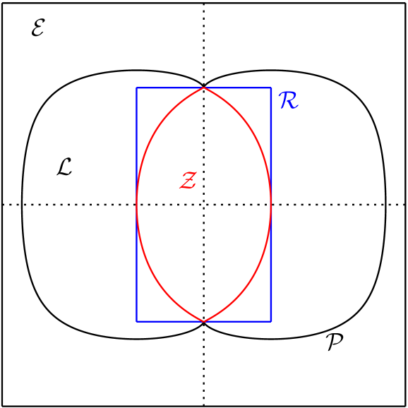
Figure 4: The parameter space, with the parabolicity curve $\mathcal{P}$ and the regions $\mathcal{E}$, $\mathcal{L}$. The region $\mathcal{Z}$ is the central region, which is contained in the rectangle $\mathcal{R}$.

The following proposition characterises those points $(\alpha_{1},\alpha_{2})$ that lie in $\mathcal{Z}$.

Proposition 4.3.

A parameter $(\alpha_{1},\alpha_{2})\in\mathcal{R}$ is in $\mathcal{Z}$ if and only if it satisfies

$$\mathcal{D}(x_{1}^{4},x_{2}^{4})=\mathcal{D}\bigl{(}4\cos^{2}(\alpha_{1}),4\cos^{2}(\alpha_{1})\bigr{)}>0,$$

where $\mathcal{D}$ is the polynomial given by

$$\mathcal{D}(x,y)=x^{3}y^{3}-9x^{2}y^{2}-27xy^{2}+81xy-27x-27.$$

The region $\mathcal{Z}$ is depicted in Figure 4: it is the interior of the central region of the figure. In fact, $\mathcal{Z}$ is the region in all of $\mathcal{L}$ where $\mathcal{I}_{0}^{+}\cap\mathcal{I}_{-1}^{-}\cap\mathcal{I}_{0}^{-}$ is empty, but as proving this is more involved, we restrict ourselves to the rectangle $\mathcal{R}$. This provides a priori bounds on the parameters $\alpha_{1}$ and $\alpha_{2}$ that will make our computations easier. We will prove Proposition 4.3 in Section 7.3. It relies on Proposition 4.4, describing the set of points where $\mathcal{D}(x_{1}^{4},x_{2}^{4})>0$ and on Proposition 4.5, which gives geometric properties of the triple intersection. Proofs of Proposition 4.4 and Proposition 4.5 will be given in Section 7.2 and Section 7.1 respectively.

Proposition 4.4.

The region $\mathcal{Z}$ is an open topological disc in $\mathcal{R}$, symmetric about the axes and intersecting them in the intervals $\{\alpha_{2}=0,\,-\pi/6<\alpha_{1}<\pi/6\}$ and $\{\alpha_{1}=0,\,-\alpha_{2}^{\lim}<\alpha_{2}<\alpha_{2}^{\lim}\}$.

Moreover, the intersection of the closure of $\mathcal{Z}$ with the parabolicity curve $\mathcal{P}$ consists of the two points $(0,\pm\alpha_{2}^{\lim})$.

Proposition 4.5.

1. The triple intersection $\mathcal{I}_{0}^{+}\cap\mathcal{I}_{0}^{-}\cap\mathcal{I}_{-1}^{-}$ is contained in the meridian $\mathfrak{m}$ of $\mathcal{I}_{0}^{+}$ defined in geographical coordinates by $\beta=(\pi-\alpha_{1})/2$.

2. If the triple intersection $\mathcal{I}_{0}^{+}\cap\mathcal{I}_{0}^{-}\cap\mathcal{I}_{-1}^{-}$ is non-empty, it contains a point in $\partial\mathbf{H}^{2}_{\mathbb{C}}$.

The second part of Proposition 4.5 is not true for general triples of bisectors. It will allow us to restrict ourselves to the boundary of $\mathbf{H}^{2}_{\mathbb{C}}$ to prove Proposition 4.3. Restricting ourselves to the region $\mathcal{Z}$ will considerably simplify the combinatorics of the family of isometric spheres $\{\mathcal{I}_{k}^{\pm}\ :\ k\in{\mathbb{Z}}\}$. The following fact will be crucial in our study; compare Figure 5.

Proposition 4.6.

Fix $(\alpha_{1},\alpha_{2})$ a point in $\mathcal{Z}$. Then the isometric sphere $\mathcal{I}_{0}^{+}$ is contained in the exterior of the isometric spheres $\mathcal{I}_{k}^{\pm}$ for all $k$, except for $\mathcal{I}_{1}^{+}$, $\mathcal{I}_{-1}^{+}$, $\mathcal{I}_{0}^{-}$ and $\mathcal{I}_{-1}^{-}$.

The proof of Proposition 4.6 will be detailed in Section 7.4. We can give more information about the intersections $\mathcal{I}_{0}^{\pm}$ with these four other isometric spheres; compare Figure 5.

Proposition 4.7.

If $(\alpha_{1},\alpha_{2})\in\mathcal{Z}$, then the intersection $\mathcal{I}_{-1}^{-}\cap\mathcal{I}_{0}^{-}$ is contained in the interior of $\mathcal{I}_{0}^{+}$.

Proof.

Since the point $p_{B}$ is the centre of $\mathcal{I}_{0}^{+}$, it lies in its interior. Moreover, $p_{B}$ lies on both $\mathcal{I}_{-1}^{-}$ and $\mathcal{I}_{0}^{-}$: indeed, $\langle{\bf p}_{AB},{\bf p}_{B}\rangle=\langle{\bf p}_{BA},{\bf p}_{B}\rangle=1$. By convexity of Cygan spheres (see Proposition 2.8), the intersection of the latter two isometric spheres is connected. This implies that $\mathcal{I}_{-1}^{-}\cap\mathcal{I}_{0}^{-}$ is contained in the interior of $\mathcal{I}_{0}^{+}$ for otherwise $\mathcal{I}_{0}^{+}\cap\mathcal{I}_{-1}^{-}\cap\mathcal{I}_{0}^{-}$ would not be empty. ∎

Using Proposition 4.2, applying powers of $\varphi$ to Propositions 4.6 and 4.7 gives the following results describing all pairwise intersections.

Corollary 4.8.

Fix $(\alpha_{1},\alpha_{2})\in\mathcal{Z}$. Then for all $k\in{\mathbb{Z}}$:

1. $\mathcal{I}_{k}^{+}$ is contained in the exterior of all isometric spheres in $\{\mathcal{I}_{k}^{\pm}\ :\ k\in{\mathbb{Z}}\}$ except $\mathcal{I}_{k-1}^{+}$, $\mathcal{I}_{k-1}^{-}$, $\mathcal{I}_{k}^{-}$ and $\mathcal{I}_{k+1}^{+}$. Moreover, $\mathcal{I}_{k}^{+}\cap\mathcal{I}_{k-1}^{-}\cap\mathcal{I}_{k}^{-}=\emptyset$ and $\mathcal{I}_{k}^{+}\cap\mathcal{I}_{k-1}^{+}$ (respectively $\mathcal{I}_{k}^{+}\cap\mathcal{I}_{k+1}^{+}$) is contained in the interior of $\mathcal{I}_{k-1}^{-}$ (respectively $\mathcal{I}_{k}^{-}$).

2. $\mathcal{I}_{k}^{-}$ is contained in the exterior of all isometric spheres in $\{\mathcal{I}_{k}^{\pm}\ :\ k\in{\mathbb{Z}}\}$ except $\mathcal{I}_{k-1}^{-}$, $\mathcal{I}_{k}^{+}$, $\mathcal{I}_{k+1}^{+}$, and $\mathcal{I}_{k+1}^{-}$. Moreover, $\mathcal{I}_{k}^{-}\cap\mathcal{I}_{k}^{-}\cap\mathcal{I}_{k+1}^{-}=\emptyset$ and $\mathcal{I}_{k}^{-}\cap\mathcal{I}_{k-1}^{-}$ (respectively $\mathcal{I}_{k}^{-}\cap\mathcal{I}_{k+1}^{-}$) is contained in the interior of $\mathcal{I}_{k}^{+}$ (respectively $\mathcal{I}_{k+1}^{+}$).

Proposition 4.6 and Corollary 4.8 are illustrated in Figure 5.

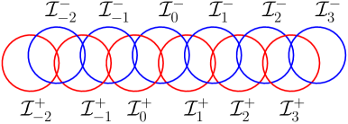
Figure 5: Vertical projections of the isometric spheres $\mathcal{I}_{k}^{\pm}$ for small values of $k$ at the point $(\alpha_{1},\alpha_{2})=(0.4,0.3)$

5 Applying the Poincaré polyhedron theorem inside $\mathcal{Z}$.

5.1 The Poincaré polyhedron theorem

For the proof of our main result we need to use the Poincaré polyhedron theorem for coset decompositions. The general principle of this result is described in Section 9.6 of [2] in the context of the Poincaré disc. A generalisation to the case of $\mathbf{H}^{2}_{\mathbb{C}}$ has already appeared in Mostow [22] and Deraux, Parker, Paupert [9]. In these cases it was assumed that the stabiliser of the polyhedron is finite. In our case the stabiliser is the infinite cyclic group generated by the unipotent parabolic map $A$. There are two main differences from the version given in [9]. First, we allow the polyhedron $D$ to have infinitely many facets, the stabiliser group $\Upsilon$ is also infinite, but we require that there are only finitely many $\Upsilon$-orbits of facets. Secondly, we consider polyhedra $D$ whose boundary intersects $\partial\mathbf{H}^{2}_{\mathbb{C}}$ in an open set, which we refer to as the ideal boundary of $D$. In fact, the version we need has many things in common with the version given by Parker, Wang and Xie [26]. A more general statement will appear in Parker’s book [24]. In what follows we will adapt our statement of the Poincaré theorem to the case we have in mind.

The polyhedron and its cell structure

Let $D$ be an open polyhedron in $\mathbf{H}^{2}_{\mathbb{C}}$ and let $\overline{D}$ denote its closure in $\overline{\mathbf{H}^{2}_{\mathbb{C}}}=\mathbf{H}^{2}_{\mathbb{C}}\cup\partial\mathbf{H}^{2}_{\mathbb{C}}$. We define the ideal boundary $\partial_{\infty}D$ of $D$ to be the intersection of $\overline{D}$ with $\partial\mathbf{H}^{2}_{\mathbb{C}}$. This polyhedron has a natural cell structure which we suppose is locally finite inside $\mathbf{H}^{2}_{\mathbb{C}}$. We suppose that the facets of $D$ of all dimensions are piecewise smooth submanifolds of $\overline{\mathbf{H}^{2}_{\mathbb{C}}}$. Let ${\mathcal{F}}_{k}(D)$ be the collection of facets of codimension $k$ having non-trivial intersection with $\mathbf{H}^{2}_{\mathbb{C}}$. We suppose that facets are closed subsets of $\overline{\mathbf{H}^{2}_{\mathbb{C}}}$. We write $f^{\circ}$ to denote the interior of a facet $f$, that is the collection of points of $f$ that are not contained in $\partial\mathbf{H}^{2}_{\mathbb{C}}$ or any facet of a lower dimension (higher codimension). Elements of ${\mathcal{F}}_{1}(D)$ and ${\mathcal{F}}_{2}(D)$ are respectively called sides and ridges of $D$. Since $D$ is a polyhedron, ${\mathcal{F}}_{0}(D)=\overline{D}$ and each ridge in ${\mathcal{F}}_{2}(D)$ lies in exactly two sides in ${\mathcal{F}}_{1}(D)$. Similarly, the intersection of facets of $D$ with $\partial\mathbf{H}^{2}_{\mathbb{C}}$ gives rise to a polyhedral structure on a subset of $\partial_{\infty}D$. We let ${\mathcal{IF}}_{k}(D)$ denote the ideal facets of $\partial_{\infty}D$ of codimension $k$ so that each facet in ${\mathcal{IF}}_{k}(D)$ is contained in some facet of ${\mathcal{F}}_{\ell}(D)$ with $\ell<k$. In particular, we will also need to consider ideal vertices in ${\mathcal{IF}}_{4}(D)$. These are points of either the endpoints of facets in ${\mathcal{F}}_{3}(D)$ or else they are points of $\partial\mathbf{H}^{2}_{\mathbb{C}}$ contained in (at least) two facets of $D$ that do not intersect inside $\mathbf{H}^{2}_{\mathbb{C}}$. Note that, since we have defined ideal facets to be subsets of facets, it may be that $\partial\mathbf{H}^{2}_{\mathbb{C}}$ contains points of $\partial_{\infty}D$ not contained in any ideal facet. In the case we consider, there will be one such point, namely the point at $\infty$ fixed by $A$.

The side pairing.

We suppose that there is a side pairing $\sigma:{\mathcal{F}}_{1}(D)\longrightarrow\mbox{\rm PU(2,1)}$ satisfying the following conditions:

1. For each side $s\in{\mathcal{F}}_{1}(D)$ with $\sigma(s)=S$ there is another side $s^{-}\in{\mathcal{F}}_{1}(D)$ so that $S$ maps $s$ homeomorphically onto $s^{-}$ preserving the cell structure. Moreover, $\sigma(s^{-})=S^{-1}$. Furthermore, if $s=s^{-}$ then $S=S^{-1}$ and $S$ is an involution. In this case, we call $S^{2}=id$ a reflection relation.

2. For each $s\in{\mathcal{F}}_{1}(D)$ with $\sigma(s)=S$ we have $\overline{D}\cap S^{-1}(\overline{D})=s$ and $D\cap S^{-1}(D)=\emptyset$.

3. For each $w$ in the interior $s^{\circ}$ of $s$ there is an open neighbourhood $U(w)\subset\mathbf{H}^{2}_{\mathbb{C}}$ of $w$ contained in $\overline{D}\cup S^{-1}(\overline{D})$.

In the example we consider, $D$ will be the Ford domain of a group. In particular, each side $s$ will be contained in the isometric sphere $\mathcal{I}(S)$ of $S=\sigma(s)$. Indeed, $s=\mathcal{I}(S)\cap\overline{D}$. By construction we have $S:\mathcal{I}(S)\longmapsto\mathcal{I}(S^{-1})$ and in this case $s^{-}=\mathcal{I}(S^{-1})\cap\overline{D}$. The polyhedron $D$ will be the (open) infinite sided polyhedron formed by the intersection of the exteriors of all the $\mathcal{I}(S)$ where $S=\sigma(s)$ and $s$ varies over ${\mathcal{F}}_{1}(D)$. By construction, the sides of $D$ are smooth hypersurfaces (with boundary) in $\mathbf{H}^{2}_{\mathbb{C}}$.

Suppose that $D$ is invariant under a group $\Upsilon$ that is compatible with the side pairing map in the sense that for all $P\in\Upsilon$ and $s\in{\mathcal{F}}_{1}(D)$ we have $P(s)\in{\mathcal{F}}_{1}(D)$ and $\sigma(Ps)=P\sigma(s)P^{-1}$. We call the latter a compatibility relation. We suppose that there are finitely many $\Upsilon$-orbits of facets in each ${\mathcal{F}}_{k}(D)$. Since $P\in\Upsilon$ cannot fix a side $s\in{\mathcal{F}}_{1}(D)$ pointwise, subdividing sides if necessary, we suppose that if $P\in\Upsilon$ maps a side in ${\mathcal{F}}_{1}(D)$ to itself then $P$ is the identity. In particular, given sides $s_{1}$ and $s_{2}$ in ${\mathcal{F}}_{1}(D)$, there is at most one $P\in\Upsilon$ sending $s_{1}$ to $s_{2}$. In the example of a Ford domain $\Upsilon$ will be $\Gamma_{\infty}$, the stabiliser of the point $\infty$ in the group $\Gamma$.

Ridges and cycle relations.

Consider a ridge $r_{1}\in{\mathcal{F}}_{2}(D)$. Then, $r_{1}$ is contained in precisely two sides of $D$, say $s_{0}^{-}$ and $s_{1}$. Consider the ordered triple $(r_{1},s_{0}^{-},s_{1})$. The side pairing map $\sigma(s_{1})=S_{1}$ sends $s_{1}$ to the side $s_{1}^{-}$ preserving its cell structure. In particular, $S_{1}(r_{1})$ is a ridge of $s_{1}^{-}$, say $r_{2}$. Let $s_{2}$ be the other side containing $r_{2}$. Then we obtain a new ordered triple $(r_{2},s_{1}^{-},s_{2})$. Now apply $\sigma(s_{2})=S_{2}$ to $r_{2}$ and repeat. Because there are only finitely many $\Upsilon$-orbits of ridges, we eventually find an $m$ so that the ordered triple $(r_{m+1},s_{m}^{-},s_{m+1})=(P^{-1}r_{1},P^{-1}s_{0}^{-},P^{-1}s_{1})$ for some $P\in\Upsilon$ (note that, by hypothesis, $P$ is unique). We define a map $\rho:{\mathcal{F}}_{2}(D)\longrightarrow\mbox{\rm PU(2,1)}$ called the cycle transformation by $\rho(r_{1})=P\circ S_{m}\circ\cdots\circ S_{1}$. (Note that for any ridge $r_{1}=s_{0}^{-}\cap s_{1}$, the cycle transformation map $\rho(r_{1})=R$ depends on a choice of one of the sides $s_{0}^{-}$ and $s_{1}$. If we choose the other one then the ridge cycle becomes $R^{-1}$. This follows from the fact that then $\sigma(s_{j}^{-})=\sigma(s_{j})^{-1}$ and from the compatibility relations.) By construction, the cycle transformation $R=\rho(r_{1})$ maps the ridge $r_{1}$ to itself setwise. However, $R$ may not be the identity on $r_{1}$, nor on $\mathbf{H}^{2}_{\mathbb{C}}$. Nevertheless, we suppose that $R$ has order $n$. The relation $R^{n}=id$ is called the cycle relation associated to $r_{1}$.

Writing the cycle transformation $\rho(r_{1})=R$ in terms of $P$ and the $S_{j}$, we let ${\mathcal{C}}(r_{1})$ be the collection of suffix subwords of $R^{n}$. That is

$${\mathcal{C}}(r_{1})=\Bigl{\{}S_{j}\circ\cdots\circ S_{1}\circ R^{k}\ :\ 0\leq j\leq m-1,\ 0\leq k\leq n-1\Bigr{\}}.$$

We say that the cycle condition is satisfied at $r_{1}$ provided:

1. $$r_{1}=\bigcap_{C\in{\mathcal{C}}(r_{1})}C^{-1}(\overline{D}).$$

2. If $C_{1},\,C_{2}\in{\mathcal{C}}(r_{1})$ with $C_{1}\neq C_{2}$ then $C_{1}^{-1}(D)\cap C_{2}^{-1}(D)=\emptyset$.

3. For each $w\in r_{1}^{\circ}$ there is an open neighbourhood $U(w)$ of $w$ so that

   $$U(w)\subset\bigcup_{C\in{\mathcal{C}}(r_{1})}C^{-1}(\overline{D}).$$

Ideal vertices and consistent horoballs.

Suppose that the set ${\mathcal{IF}}_{4}(D)$ of ideal vertices of $D$ is non-empty. In our applications, there are no edges (that is ${\mathcal{F}}_{3}(D)$ is empty) and the only ideal vertices arise as points of tangency between the ideal boundaries of ridges in ${\mathcal{F}}_{2}(D)$. In order to simplify our discussion below, we will only treat this case. We require that there is a system of consistent horoballs based at the ideal vertices and their images under the side pairing maps (see page 152 of [10] for definition). For each ideal vertex $\xi\in{\mathcal{IF}}_{4}(D)$, the consistent horoball $H_{\xi}$ is a horoball based at $\xi$ with the following property. Let $\xi\in{\mathcal{IF}}_{4}(D)$ and let $s\in{\mathcal{F}}_{1}(D)$ be a side with $\xi\in s$. Then the side pairing $S=\sigma(s)$ maps $\xi$ to a point $\xi^{-}$ in $s^{-}$. Note that $\xi^{-}$ is not necessarily an ideal vertex (since it could be that $\xi$ is a point of tangency between two sides whose closures in $\overline{\mathbf{H}^{2}_{\mathbb{C}}}$ are otherwise disjoint and $\xi^{-}$ may be a point of tangency between two nested bisectors only one of which contributes a side of $D$). In our case this does not happen and so we may assume $\xi^{-}$ also lies in ${\mathcal{IF}}_{4}(D)$ and so has a consistent horoball $H_{\xi^{-}}$. In order for these horoballs to form a system of consistent horoballs we require that for each ideal vertex $\xi$ and each side $s$ with $\xi\in s$ the side pairing map $\sigma(s)$ should map the horoball $H_{\xi}$ onto the horoball $H_{\xi^{-}}$. In particular, any cycle of side pairing maps sending $\xi$ to itself must also send $H_{\xi}$ to itself.

Statement of the Poincaré polyhedron theorem.

We can now state the version of the Poincaré polyhedron theorem that we need (compare [22] or [9]).

Theorem 5.1.

Let $D$ be a smoothly embedded polyhedron $D$ in $\mathbf{H}^{2}_{\mathbb{C}}$ together with a side pairing $\sigma:{\mathcal{F}}_{1}(D)\longrightarrow\mbox{\rm PU(2,1)}$. Let $\Upsilon<\mbox{\rm PU(2,1)}$ be a group of automorphisms of $D$ compatible with the side pairing and suppose that each ${\mathcal{F}}_{k}(D)$ contains finitely many $\Upsilon$-orbits. Fix a presentation for $\Upsilon$ with generating set ${\mathcal{P}}_{\upsilon}$ and relations ${\mathcal{R}}_{\Upsilon}$. Let $\Gamma$ be the group generated by ${\mathcal{P}}_{\Upsilon}$ and the side pairing maps $\{\sigma(s)\}$. Suppose that the cycle condition is satisfied for each ridge in ${\mathcal{F}}_{2}(D)$ and that there is a system of consistent horoballs at all the ideal vertices of $D$ (if any). Then:

1. The images of $D$ under the cosets of $\Upsilon$ in $\Gamma$ tessellate $\mathbf{H}^{2}_{\mathbb{C}}$. That is $\mathbf{H}^{2}_{\mathbb{C}}\subset\bigcup_{A\in\Gamma}A(\overline{D})$ and $D\cap A(D)=\emptyset$ for all $A\in\Gamma-\Upsilon$.

2. The group $\Gamma$ is discrete and a fundamental domain for its action on $\mathbf{H}^{2}_{\mathbb{C}}$ is obtained from the intersection of $D$ with a fundamental domain for $\Upsilon$.

3. A presentation for $\Gamma$ (with respect to the generating set ${\mathcal{P}}_{\Upsilon}\cup\{\sigma(s)\}$) has the following set of relations: the relations ${\mathcal{R}}_{\Upsilon}$ in $\Upsilon$, the compatibility relations between $\sigma$ and $\Upsilon$, the reflection relations and the cycle relations.

5.2 Application to our examples.

We are now going to apply Theorem 5.1 to the group generated by $S$ and $A$. Explicit matrices for these transformations are provided in equations (13) and (16). Our aim is to prove:

Theorem 5.2.

Suppose that $(\alpha_{1},\alpha_{2})$ is in $\mathcal{Z}$. That is, $\mathcal{D}\bigl{(}4\cos^{2}(\alpha_{1}),4\cos^{2}(\alpha_{1})\bigr{)}>0$, where $\mathcal{D}(x,y)$ is the polynomial defined in Proposition 4.3. Then the group $\Gamma=\langle S,A\rangle$ associated to the parameters $(\alpha_{1},\alpha_{2})$ is discrete and has the presentation

$$\langle S,\,A\ :\ S^{3}=(A^{-1}S)^{3}=id\rangle.$$ (20)

We obtain the presentation $\langle S,\,T\ :\ S^{3}=T^{3}=id\rangle$ by changing generators to $S$ and $T=A^{-1}S$.

Definition of the polyhedron and its cell structure.

The infinite polyhedron we consider is the intersection of the exteriors of all the isometric spheres in $\{\mathcal{I}_{k}^{\pm}\ :\ k\in{\mathbb{Z}}\}$.

Definition 8.

We call $D$ the intersection of the exteriors of all isometric spheres $\mathcal{I}_{k}^{+}$ and $\mathcal{I}_{k}^{-}$ with centres $A^{k}S^{-1}(q_{\infty})$ and $A^{k}S(q_{\infty})$ respectively :

$$D=\Bigl{\{}q\in\mathbf{H}^{2}_{\mathbb{C}}\ :\ d_{\rm Cyg}\bigl{(}q,A^{k}S^{\pm 1}(q_{\infty})\bigr{)}>1\hbox{ for all }k\in{\mathbb{Z}}\Bigr{\}}.$$ (21)

The set of sides of $D$ is ${\mathcal{F}}_{1}(D)=\{s_{k}^{+},\,s_{k}^{-}\ :\ k\in{\mathbb{Z}}\}$ where $s_{k}^{+}=\mathcal{I}_{k}^{+}\cap\overline{D}$ and $s_{k}^{-}=\mathcal{I}_{k}^{-}\cap\overline{D}$.

Using Corollary 4.8 we can completely describe $s_{k}^{+}$ and $s_{k}^{-}$.

Proposition 5.3.

The side $s_{k}^{\pm}$ is topologically a solid cylinder in $\mathbf{H}^{2}_{\mathbb{C}}\cup\partial\mathbf{H}^{2}_{\mathbb{C}}$. More precisely, $s_{k}^{\pm}$ is a product $D\times[0,1]$ where for each $t\in[0,1]$, the fibre $D\times\{t\}$ is homeomorphic to a closed disc in $\overline{\mathbf{H}^{2}_{\mathbb{C}}}$ whose boundary is contained in $\partial\mathbf{H}^{2}_{\mathbb{C}}$. The intersection of $\partial s_{k}^{+}$ (respectively $\partial s_{k}^{-}$) with $\mathbf{H}^{2}_{\mathbb{C}}$ is the disjoint union of the topological discs $s_{k}^{+}\cap s_{k-1}^{-}$ and $s_{k}^{+}\cap s_{k}^{-}$ (respectively $s_{k}^{-}\cap s_{k}^{+}$ and $s_{k}^{-}\cap s_{k+1}^{-}$).

Proof.

Since $s_{k}^{+}$ is contained in $\mathcal{I}_{k}^{+}$, its only possible intersections with other sides are contained in $\mathcal{I}_{k-1}^{+}$, $\mathcal{I}_{k-1}^{-}$, $\mathcal{I}_{k+1}^{+}$ and $\mathcal{I}_{k+1}^{-}$ by Corollary 4.8. Since $\mathcal{I}_{k}^{+}\cap\mathcal{I}_{k-1}^{+}$ and $\mathcal{I}_{k}^{+}\cap\mathcal{I}_{k+1}^{+}$ are contained in the interiors of other isometric spheres, the intersections $s_{k}^{+}\cap s_{k-1}^{+}$ and $s_{k}^{+}\cap s_{k+1}^{+}$ are empty. Also, $\mathcal{I}_{k}^{+}\cap\mathcal{I}_{k-1}^{-}\cap\mathcal{I}_{k}^{-}=\emptyset$ and so $s_{k}^{+}\cap s_{k-1}^{-}$ and $s_{k}^{+}\cap s_{k}^{-}$ are disjoint. Since isometric spheres are topological balls and their pairwise intersections are connected, the description of $s_{k}^{+}$ follows. A similar argument describes $s_{k}^{-}$. ∎

The side pairing $\sigma:{\mathcal{F}}_{1}(D)\longrightarrow\mbox{\rm PU(2,1)}$ is defined by

$$\sigma(s_{k}^{+})=A^{k}SA^{-k},\qquad\sigma(s_{k}^{-})=A^{k}S^{-1}A^{-k}.$$ (22)

Let $\Upsilon=\langle A\rangle$ be the infinite cyclic group generated by $A$. By construction the side pairing $\sigma$ is compatible with $\Upsilon$. Furthermore, using Proposition 5.3 the set of ridges is ${\mathcal{F}}_{2}(D)=\{r_{k}^{+},\,r_{k}^{-}\ :\ k\in{\mathbb{Z}}\}$ where $r_{k}^{+}=s_{k}^{+}\cap s_{k}^{-}$ and $r_{k}^{-}=s_{k}^{+}\cap s_{k-1}^{-}$. We can now verify that $\sigma$ satisfies the first condition of being a side pairing.

Proposition 5.4.

The side pairing map $\sigma(s_{k}^{+})=A^{k}SA^{-k}$ is a homeomorphism from $s_{k}^{+}$ to $s_{k}^{-}$. Moreover $\sigma(s_{k}^{-})$ sends $r_{k}^{+}=s_{k}^{+}\cap s_{k}^{-}$ to itself and sends $r_{k}^{-}=s_{k}^{+}\cap s_{k-1}^{-}$ to $r_{k+1}^{-}=s_{k}^{-}\cap s_{k+1}^{+}$.

Proof.

By applying powers of $A$ we need only need to consider the case where $k=0$. First, the ridge $r_{0}^{+}=s_{0}^{+}\cap s_{0}^{-}=\mathcal{I}(S)\cap\mathcal{I}(S^{-1})$ is defined by the triple equality

$$|\langle{\bf z},{\bf q}_{\infty}\rangle|=|\langle{\bf z},S^{-1}{\bf q}_{\infty}\rangle|=|\langle{\bf z},S{\bf q}_{\infty}\rangle|.$$ (23)

The map $S$ cyclically permutes $p_{B}=S^{-1}(q_{\infty})$, $p_{A}=q_{\infty}$, $p_{AB}=S(q_{\infty})$, and so maps $r_{0}^{+}$ to itself. Similarly, consider $r_{0}^{-}=s_{0}^{+}\cap s_{-1}^{-}$. The side pairing map $S$ sends $A^{-1}S(q_{\infty})$, the centre of $\mathcal{I}_{-1}^{-}$, to

$$S(A^{-1}S)(q_{\infty})=S(T^{-1}S^{-1})S(q_{\infty})=ST^{2}(q_{\infty})=(ST)S^{-1}(ST)(q_{\infty})=AS^{-1}(q_{\infty}),$$

which is the centre of $\mathcal{I}_{1}^{+}$, where we have used $A^{-1}=T^{-1}S^{-1}$, $T^{-1}=T^{2}$ and $ST(q_{\infty})=q_{\infty}$. Therefore $r_{0}^{-}=s_{0}^{+}\cap s_{-1}^{-}$ is sent to $r_{1}^{-}=s_{0}^{-}\cap s_{1}^{+}$ as claimed. The rest of the result follows from our description of $s_{k}^{\pm}$ in Proposition 5.3. ∎

Local tessellation.

We now prove local tessellation around the sides and ridges of $D$.

• Since $\sigma(s_{k}^{\pm})=A^{k}S^{\pm 1}A^{-1}$ sends the exterior of $\mathcal{I}_{k}^{\pm}$ to the interior of $\mathcal{I}_{k}^{\mp}$ we see that $D$ and $A^{k}S^{\pm 1}A^{-k}(D)$ have disjoint interiors and cover a neighbourhood of each point in $s_{k}^{\mp}$. Together with Proposition 5.4 this means $\sigma$ satisfies the three conditions of being a side pairing.

• Consider the case of $r_{0}^{+}=s_{0}^{+}\cap s_{0}^{-}=\mathcal{I}(S)\cap\mathcal{I}(S^{-1})$, which is given by (23). Observe that $r_{0}^{+}$ is mapped to itself by $S$. Using Proposition 5.4, we see that when constructing the cycle transformation for $r_{0}^{+}$ we have one ordered triple $(r_{0}^{+},s_{0}^{-},s_{0}^{+})$ and the cycle transformation $\rho(r_{0}^{+})=S$. The cycle relation is $S^{3}=id$ and ${\mathcal{C}}(r_{0}^{+})=\{id,\,S,\,S^{2}\}$. Consider an open neighbourhood $U_{0}^{+}$ of $r_{0}^{+}$ but not intersecting any other ridge. The intersection of $D$ with $U_{0}^{+}$ is the same as the intersection of $U_{0}^{+}$ with the Ford domain $D_{S}$ for the order three group $\langle S\rangle$. Since $S$ has order 3 this Ford domain is the intersection of the exteriors of $\mathcal{I}(S)$ and $\mathcal{I}(S^{-1})$. For $z$ in $D_{S}$, $|\langle{\bf z},{\bf q}_{\infty}\rangle|$ is the smallest of the three quantities in (23). Applying $S=\sigma(s_{0}^{+})$ and $S^{-1}=\sigma(s_{0}^{-})$ gives regions $S(D_{S})$ and $S^{-1}(D_{S})$ where one of the other two quantities is the smallest. Therefore $U_{0}^{+}\cap S(U_{0}^{+})\cap S(U_{0}^{-})$ is an open neighbourhood of $r_{0}^{+}$ contained in $D\cup S(D)\cup S^{-1}(D)$. This proves the cycle condition at $r_{0}^{+}$.

• Now consider $r_{0}^{-}=s_{0}^{+}\cap s_{-1}^{-}$. When constructing the cycle transformation for $r_{0}^{-}$ we start with the ordered triple $(r_{0}^{-},s_{-1}^{-},s_{0}^{+})$. Applying $S=\sigma(s_{0}^{+})$ to $r_{0}^{-}$ gives the ordered triple $(r_{1}^{-},s_{0}^{-},s_{1}^{+})$, which is simply $(Ar_{0}^{-},As_{-1}^{-},As_{0}^{+})$. Thus the cycle transformation of $r_{0}^{-}$ is $\rho(r_{0}^{-})=A^{-1}S=T^{-1}$, which has order 3. Therefore the cycle relation is $(A^{-1}S)^{3}=id$, and ${\mathcal{C}}(r_{0}^{-})=\{id,\,A^{-1}S,\,(A^{-1}S)^{2}\}$. Noting that $\mathcal{I}_{0}^{+}$ has centre $S^{-1}(q_{\infty})S^{-1}A(q_{\infty})=T(q_{\infty})$ and $\mathcal{I}_{-1}^{-}$ has centre $A^{-1}S(q_{\infty})=T^{-1}(q-\infty)$ we see $\mathcal{I}_{0}^{+}=\mathcal{I}(T^{-1})$ and $\mathcal{I}_{0}^{-}=\mathcal{I}(T)$. Therefore a similar argument involving the Ford domain for $\langle T\rangle$ shows that the cycle condition is satisfied at $r_{0}^{-}$.

• Using compatibility of the side pairings with $\Upsilon=\langle A\rangle$, we see that $\rho(r_{k}^{+})=A^{k}SA^{-k}$ with cycle relation $(A^{k}SA^{-k})^{3}=A^{k}S^{3}A^{-k}=id$ and that the cycle condition is satisfied at $r_{k}^{+}$. Likewise, $\rho(r_{k}^{-})=A^{k}(A^{-1}S)A^{-k}=A^{k-1}SA^{-k}$ with cycle relation $(A^{k-1}SA^{-k})^{3}=A^{k}(A^{-1}S)A^{-k}=id$ and the cycle condition is satisfied at $r_{k}^{-}$.

This is sufficient to prove Theorem 5.2 by applying the Poincaré polyhedron theorem when $D$ has no ideal vertices, that is to all groups $\Gamma$ in the interior of ${\mathcal{Z}}$. In particular, $\Gamma$ is generated by the generator $A$ of $\Upsilon$ and the side pairing maps. Using the compatibility relations, there is only one side pairing map up to the action of $\Upsilon$, namely $S$. There are no reflection relations, and (again up to the action of $\Upsilon$) the only cycle relations are $S^{3}=id$ and $(A^{-1}S)^{3}=id$. Thus the Poincaré polyhedron theorem gives the presentation (20). This completes the proof of Theorem 5.2.

For groups on the boundary of $\mathcal{Z}$ the same result is also true. This follows from the fact (Chuckrow’s theorem): the algebraic limit of a sequence of discrete and faithful representations of a non virtually nilpotent group in Isom($\mathbf{H}^{n}_{\mathbb{C}}$) is discrete and faithful (see for instance Theorem 2.7 of [4] or [21] for a more general result in the frame of negatively curved groups).

We do not need to apply the Poincaré polyhedron theorem for these groups. However, to describe the manifold at infinity for the limit groups, we will need to know a fundamental domain, and we will have to go through a similar analysis in the next section.

6 The limit group.

In this section, we consider the group $\Gamma^{\lim}$, and unless otherwise stated, the parameters $\alpha_{1}$ and $\alpha_{2}$ will always be assumed to be equal to $0$ and $\alpha_{2}^{\lim}$ respectively. We know already that $\Gamma^{\lim}$ is discrete and isomorphic to ${\mathbb{Z}}_{3}\ast{\mathbb{Z}}_{3}$. Our goal is to prove that its manifold at infinity is homeomorphic to the complement of the Whitehead link. For these values of the parameters, the maps $S^{-1}T$ and $ST^{-1}$ are unipotent parabolic (see the results of Section 3.4), and we denote by $V_{S^{-1}T}$ and $V_{ST^{-1}}$ respectively the sets of (parabolic) fixed points of conjugates of $S^{-1}T$ and $ST^{-1}$ by powers of $A$.

1. As in the previous section, we apply the Poincaré polyhedron theorem, this time to the group $\Gamma^{\lim}$. We obtain an infinite $A$-invariant polyhedron, still denoted $D$, which is a fundamental domain for $A$-cosets. This polyhedron is slightly more complicated than the one in the previous section due to the appearance of ideal vertices that are the points in $V_{S^{-1}T}$ and $V_{ST^{-1}}$.

2. We analyse the combinatorics of the ideal boundary $\partial_{\infty}D$ of this polyhedron. More precisely, we will see that the quotient of $\partial_{\infty}D\setminus\left(\{p_{A}\}\cup V_{S^{-1}T}\cup V_{ST^{-1}}\right)$ by the action of the group $\langle S,T\rangle$ is homeomorphic the complement of the Whitehead link, as stated in Theorem 6.4.

6.1 Matrices and fixed points.

Before going any further, we provide specific expressions for the various objects we consider at the limit point. When $\alpha_{1}=0$ and $\alpha_{2}=\alpha_{2}^{\lim}$, the map $\varphi$ described in Proposition 4.2 is given in Heisenberg coordinates by

$$\varphi:[z,t]\longmapsto\left[\overline{z}+\sqrt{3/8}+i\sqrt{5/8},-t+x\sqrt{5/2}+y\sqrt{3/2}\right].$$ (24)

In particular its invariant line $\Delta_{\varphi}$ is parametrised by

$$\Delta_{\varphi}=\Bigl{\{}\delta_{\varphi}(x)=\left[\,x+i\sqrt{5/32},\,x\sqrt{5/8}\,\right]\ :\ x\in\mathbb{R}\Bigr{\}}.$$ (25)

The parabolic map $A=\varphi^{2}$ acts on $\Delta_{\varphi}$ as $A:\delta_{\varphi}(x)\longmapsto\delta_{\varphi}(x+\sqrt{3/2})$. As a matrix it is given by

$$A=\begin{bmatrix}1&-\sqrt{3}&-3/2+i\sqrt{15}/2\\ 0&1&\sqrt{3}\\ 0&0&1\end{bmatrix}.$$ (26)

We can decompose $A$ into the product of regular elliptic maps $S$ and $T$:

$$S=\begin{bmatrix}1&\sqrt{3}/2-i\sqrt{5}/2&-1\\ -\sqrt{3}/2-i\sqrt{5}/2&-1&0\\ -1&0&0\end{bmatrix},\quad T=\begin{bmatrix}0&0&-1\\ 0&-1&-\sqrt{3}/2+i\sqrt{5}/2\\ -1&\sqrt{3}/2+i\sqrt{5}/2&1\end{bmatrix}$$

These maps cyclically permute $(p_{A},p_{AB},p_{B})$ and $(p_{A},p_{B},p_{BA})$ where

$${\bf p}_{A}=\begin{bmatrix}1\\ 0\\ 0\end{bmatrix},\quad{\bf p}_{B}=\begin{bmatrix}0\\ 0\\ 1\end{bmatrix},\quad{\bf p}_{AB}=\begin{bmatrix}-1\\ \sqrt{3}/2+i\sqrt{5/2}\\ 1\end{bmatrix},\quad{\bf p}_{BA}=\begin{bmatrix}-1\\ -\sqrt{3}/2+i\sqrt{5}/2\\ 1\end{bmatrix}.$$ (27)

Using $\alpha_{1}=0$, we will occasionally use the facts from Proposition 3.6 that $(S,T)$ is $\mathbb{C}$-decomposable and $(A,B)$ is $\mathbb{R}$-decomposable.

As mentioned above, in the group $\Gamma^{\lim}$ the elements $ST^{-1}$, $S^{-1}T$, $TST$, $STS$ and the commutator $[A,B]=(ST^{-1})^{3}$ are unipotent parabolic. For future reference, we provide here lifts of their fixed points, both as vectors in $\mathbb{C}^{3}$ and in terms of geographical coordinates $g(\alpha,\beta)$ (we omit the $w$ coordinates: since we are on the boundary at infinity, it is equal to $\sqrt{2\cos\alpha}$).

$${\bf p}_{ST^{-1}} = \begin{bmatrix}-1/4+i\sqrt{15}/4\\ \sqrt{3}/4+i\sqrt{5}/4\\ 1\end{bmatrix}\ =\ {\bf g}\left(\arccos(1/4),\pi/2\right),$$

$${\bf p}_{S^{-1}T} = \begin{bmatrix}-1/4-i\sqrt{15}/4\\ -\sqrt{3}/4+i\sqrt{5}/4\\ 1\end{bmatrix}\ =\ {\bf g}\left(-\arccos(1/4),\pi/2\right),$$

$${\bf p}_{TST} = \begin{bmatrix}-1\\ -3\sqrt{3}/4+i\sqrt{5}/4\\ 1\end{bmatrix}\ =\ {\bf g}\left(0,-\arccos\left(\sqrt{27/32}\right)\right),$$

$${\bf p}_{STS} = \begin{bmatrix}-1\\ 3\sqrt{3}/4+i\sqrt{5}/4\\ 1\end{bmatrix}\ =\ {\bf g}\left(0,\arccos\left(\sqrt{27/32}\right)\right).$$ (28)

It follows from (24) that $\varphi$ acts on these parabolic fixed points as follows:

$$\cdots p_{T^{-1}STST}\overset{\varphi}{\longrightarrow}p_{TST}\overset{\varphi}{\longrightarrow}p_{S^{-1}T}\overset{\varphi}{\longrightarrow}p_{ST^{-1}}\overset{\varphi}{\longrightarrow}p_{STS}\overset{\varphi}{\longrightarrow}p_{STSTS^{-1}}\cdots$$ (29)

6.2 The Poincaré theorem for the limit group.

The limit group has extra parabolic elements. Therefore, in order to apply the Poincaré theorem, we must construct a system of consistent horoballs at these parabolic fixed points (see Section 5.1).

Lemma 6.1.

The isometric spheres $\mathcal{I}_{1}^{+}$ and $\mathcal{I}_{-1}^{-}$ are tangent at $p_{ST^{-1}}$. The isometric spheres $\mathcal{I}_{-1}^{+}$ and $\mathcal{I}_{0}^{-}$ are tangent at $p_{S^{-1}T}$.

Proof.

It is straightforward to verify that $|\langle{\bf p}_{ST^{-1}},{\bf p}_{BA}\rangle|=|\langle{\bf p}_{ST^{-1}},A({\bf p}_{B})\rangle|=1$, and therefore $p_{ST^{-1}}$ belongs to both $\mathcal{I}_{-1}^{-}$ and $\mathcal{I}_{1}^{+}$. Projecting vertically (see Remark 1), we see that the projections of $\mathcal{I}_{-1}^{-}$ and $\mathcal{I}_{1}^{+}$ are tangent discs and as they are strictly convex, their intersection contains at most one point. This gives the result. The other tangency is along the same lines. ∎

A consequence of Lemma 6.1 is that the parabolic fixed points are tangency points of isometric spheres. The following lemma is proved in Section 7.1.

Lemma 6.2.

For the group $\Gamma^{\lim}$ the triple intersection $\mathcal{I}_{0}^{+}\cap\mathcal{I}_{0}^{-}\cap\mathcal{I}_{-1}^{-}$ contains exactly two points, namely the parabolic fixed points $p_{ST^{-1}}$ and $p_{S^{-1}T}$.

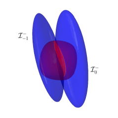
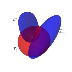
Figure 6: Two realistic views of the isometric spheres $\mathcal{I}_{0}^{+}$, $\mathcal{I}_{1}^{+}$ and $\mathcal{I}_{0}^{-}$ for the limit group $\Gamma^{\lim}$. The thin bigon is $\mathcal{B}_{0}^{+}$ (defined in Proposition 6.5). Compare with Figures 8 and 12

Applying powers of $\varphi$, we see that these triple intersections are actually quadruple intersections of sides and triple intersections of ridges.

Corollary 6.3.

The parabolic fixed point $A^{k}(p_{ST^{-1}})$ lies on $\mathcal{I}_{k-1}^{-}\cap\mathcal{I}_{k}^{+}\cap\mathcal{I}_{k}^{-}\cap\mathcal{I}_{k}^{+}$. In particular, it is the triple ridge intersection $r_{k}^{-}\cap r_{k}^{+}\cap r_{k+1}^{-}$. Similarly, $A^{k}(p_{S^{-1}T})$ lies on $\mathcal{I}_{-1}^{+}\cap\mathcal{I}_{-1}^{-}\cap\mathcal{I}_{0}^{+}\cap\mathcal{I}_{0}^{-}$. In particular it is $r_{k-1}^{+}\cap r_{k}^{-}\cap r_{k}^{+}$.

To construct a system of consistent horoballs at the parabolic fixed points we must investigate the action of the side pairing maps on them. First, $p_{S^{-1}T}\in\mathcal{I}_{-1}^{+}\cap\mathcal{I}_{-1}^{-}\cap\mathcal{I}_{0}^{+}\cap\mathcal{I}_{0}^{-}$, we have

$$\sigma(s_{-1}^{+})=A^{-1}SA:p_{S^{-1}T} \longmapsto p_{T^{-1}STST},$$

$$\sigma(s_{-1}^{-})=A^{-1}S^{-1}A:p_{S^{-1}T} \longmapsto p_{TST},$$

$$\sigma(s_{0}^{+})=S:p_{S^{-1}T} \longmapsto p_{ST^{-1}},$$

$$\sigma(s_{0}^{-})=S^{-1}:p_{S^{-1}T} \longmapsto p_{STS}.$$

Likewise $p_{ST^{-1}}\in\mathcal{I}_{-1}^{-}\cap\mathcal{I}_{0}^{+}\cap\mathcal{I}_{0}^{-}\cap\mathcal{I}_{1}^{+}$. We have

$$\sigma(s_{-1}^{-})=A^{-1}S^{-1}A:p_{ST^{-1}} \longmapsto A^{-2}(p_{ST^{-1}}),$$

$$\sigma(s_{0}^{+})=S:p_{ST^{-1}} \longmapsto p_{STS},$$

$$\sigma(s_{0}^{-})=S^{-1}:p_{ST^{-1}} \longmapsto p_{S^{-1}T},$$

$$\sigma(s_{1}^{+})=ASA^{-1}:p_{ST^{-1}} \longmapsto A^{2}(p_{ST^{-1}}).$$

We can combine these maps to show how the points $A^{k}(p_{ST^{-1}})$ and $A^{k}(p_{S^{-1}T})$ are related by the side pairing maps. This leads to an infinite graph, a section of which is:

(30)

From this it is clear that all the cycles in the graph (30) are generated by triangles and quadrilaterals. Up to powers of $A$, the triangles lead to the word $S^{3}$, which is the identity. Up to powers of $A$ the quadrilaterals lead to words cyclically equivalent to the one coming from:

In other words, $p_{S^{-1}T}$ is fixed by $(A^{-1}SA)(S^{-1})(ASA^{-1})(S^{-1})=(T^{-1}S)^{3}$. This is parabolic and so preserves all horoballs based at $p_{S^{-1}T}$.

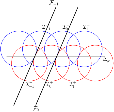
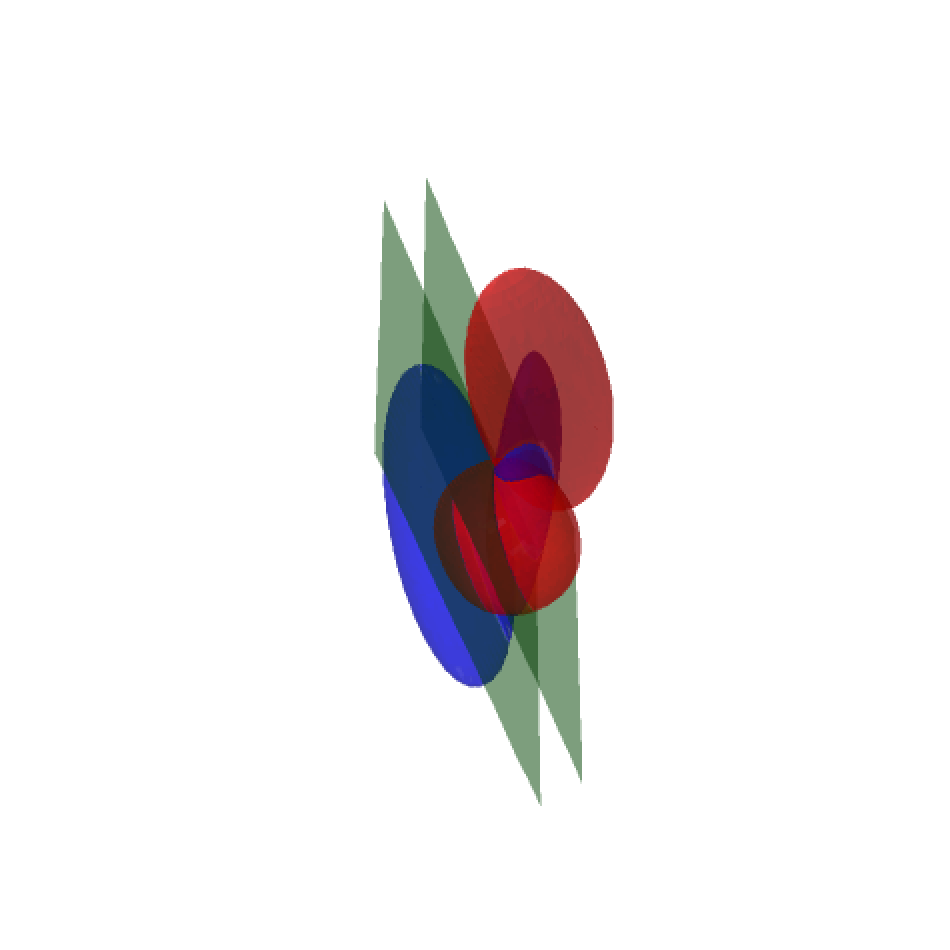
Figure 7: Vertical projection and realistic view of the isometric spheres and the fans $F_{0}$ and $F_{-1}$ for the parameter values $\alpha_{1}=0$, $\alpha_{2}=\alpha_{2}^{\lim}$. Compare with Figure 5.

Therefore, we can define a system of horoballs as follows. Let $U_{0}^{+}$ be a horoball based at $p_{S^{-1}T}$, disjoint from the closure of any side not containing $p_{S^{-1}T}$ in its closure. Now define horoballs $U_{k}^{+}$ and $U_{k}^{-}$ by applying the side pairing maps to $U_{0}^{+}$. Since every cycle in the graph (30) gives rise either to the identity map or to a parabolic map, this process is well defined and gives rise to a consistent system of horoballs. Therefore we can apply the Poincaré polyhedron theorem for the two limit groups. Using the same arguments as we did for groups in the interior of ${\mathcal{Z}}$, we see that $\Gamma$ has the presentation (20).

6.3 The boundary of the limit orbifold.

Theorem 6.4.

The manifold at infinity of the group $\Gamma^{\lim}$ is homeomorphic to the Whitehead link complement.

The ideal boundary of $D$ is made up of those pieces of the isometric spheres $\mathcal{I}_{k}^{\pm}$ that are outside all other isometric spheres in $\{\mathcal{I}_{k}^{\pm}\ :\ k\in{\mathbb{Z}}\}$. Recall that the (ideal boundary of) the side $s_{k}^{\pm}$ is the part of $\partial\mathcal{I}_{k}^{\pm}$ which is outside (the ideal boundary of) all other isometric spheres. In this section, when we speak of sides and ridges we implicitly mean their intersection with $\partial\mathbf{H}^{2}_{\mathbb{C}}$.

We will see that each isometric sphere in $\{\mathcal{I}_{k}^{\pm}\ :\ k\in{\mathbb{Z}}\}$ contributes a side $s_{k}^{\pm}$ made up of one quadrilateral, denoted by $\mathcal{Q}_{k}^{\pm}$ and one bigon $\mathcal{B}_{k}^{\pm}$. A very similar configuration of isometric spheres has been observed by Deraux and Falbel in [8]. We begin by analysing the contribution of $\mathcal{I}_{0}^{+}$.

Proposition 6.5.

The side $(s_{0}^{+})^{\circ}$ of $D$ has two connected components.

1. One of them is a quadrilateral, denoted $\mathcal{Q}_{0}^{+}$, whose vertices are points $p_{ST^{-1}}$, $p_{S^{-1}T}$, $p_{STS}$ and $p_{TST}$ (all of which are parabolic fixed points)

2. The other is a bigon, denoted $\mathcal{B}_{0}^{+}$, whose vertices are $p_{ST^{-1}}$ and $p_{S^{-1}T}$

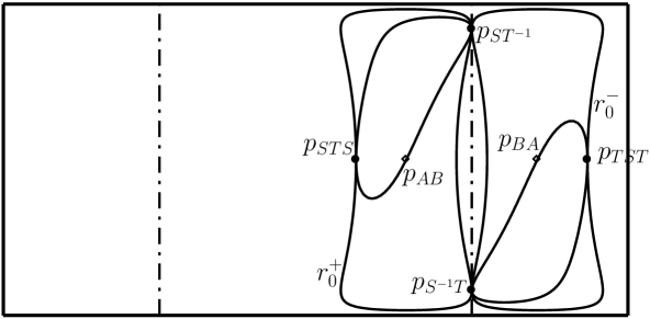
Figure 8: Intersections of the isometric spheres $\mathcal{I}_{0}^{-}$, $\mathcal{I}_{-1}^{-}$, $\mathcal{I}_{1}^{+}$ and $\mathcal{I}_{-1}^{+}$ with $\mathcal{I}_{0}^{+}$ in the boundary of $\mathbf{H}^{2}_{\mathbb{C}}$, viewed in geographical coordinates. Recall that $r_{0}^{+}=\mathcal{I}_{0}^{+}\cap\mathcal{I}_{0}^{-}$ and $r_{0}^{-}=\mathcal{I}_{0}^{+}\cap\mathcal{I}_{-1}^{-}$. Here $\alpha\in[-\pi/2,\pi/2]$ is the vertical coordinates, and $\beta\in[-\pi,\pi]$ the horizontal one. The vertical dash-dotted segments $\beta=\pm\pi/2$ are the two halves of the boundary of the meridian $\mathfrak{m}$. The bigon between the two curves $r_{0}^{+}$ and $r_{0}^{-}$ is $\mathcal{B}_{0}^{+}$ (see Proposition 6.5). Compare to Figure 2 of [8].

Proof.

Since isometric spheres are strictly convex, the ideal boundaries of the ridges $r_{0}^{+}=\mathcal{I}_{0}^{+}\cap\mathcal{I}_{0}^{-}$ and $r_{0}^{-}=\mathcal{I}_{0}^{+}\cap\mathcal{I}_{-1}^{-}$ are Jordan curves on $\mathcal{I}_{0}^{+}$. We still denote them by $r_{0}^{\pm}$. The interiors of these curves are respectively the connected components containing $p_{AB}$ and $p_{BA}$. By Lemma 6.2 in Section 7.1, $r_{0}^{+}$ and $r_{0}^{-}$ have two intersection points, namely $p_{S^{-1}T}$ and $p_{ST^{-1}}$, and their interiors are disjoint. As a consequence the common exterior of the two curves has two connected components, and the points $p_{S^{-1}T}$ and $p_{ST^{-1}}$ lie on the boundary of both.

To finish the proof, consider the involution $\iota_{1}$ defined in the proof of Proposition 3.6. (Note that since $\alpha_{1}=0$ this involution conjugates $\Gamma^{\lim}$ to itself.) In Heisenberg coordinates it is defined by $\iota_{1}:[z,t]\longmapsto[-\overline{z},-t]$ and is clearly a Cygan isometry. As in Proposition 3.6, $\iota_{1}$ fixes $p_{A}$ and $p_{B}$ and it interchanges $p_{AB}$ and $p_{BA}$. Thus it conjugates $S$ to $T^{-1}$ and so it interchanges $p_{ST^{-1}}$ and $p_{S^{-1}T}$ and it interchanges $p_{STS}$ and $p_{TST}$. Moreover, since it is a Cygan isometry, $\iota_{1}$ preserves $\mathcal{I}_{0}^{+}$ and interchanges $\mathcal{I}_{-1}^{-}$ and $\mathcal{I}_{0}^{-}$ and thus it also exchanges the two curves $r_{0}^{+}$ and $r_{0}^{-}$. Again, since it is a Cygan isometry, it maps interior to interior and exterior to exterior for both curves. As a consequence, the two connected components of the common exterior are either exchanged or both preserved.

Now consider the point with Heisenberg coordinates $[i,0]$. It is fixed by $\iota_{1}$, and belongs to the common exterior of both $r_{0}^{+}$ and $r_{0}^{-}$. This implies that both connected components are preserved. Finally, since $p_{STS}\in\mathcal{I}_{0}^{+}\cap\mathcal{I}_{0}^{-}$ and $p_{TST}\in\mathcal{I}_{0}^{+}\cap\mathcal{I}_{-1}^{-}$ are exchanged by $\iota_{1}$, these two points belong to the closure of the same connected component. As a consequence, one of the two connected components has $p_{ST^{-1}}$, $p_{S^{-1}T}$, $p_{STS}$ and $p_{TST}$ on its boundary. This is the quadrilateral. The other one has $p_{ST^{-1}}$ and $p_{S^{-1}T}$ on its boundary. This is the bigon. ∎

We now apply powers of $A$ to get a result about all the isometric sphere intersections in the ideal boundary of $D$. Define $\mathcal{Q}_{0}^{-}=\varphi(\mathcal{Q}_{0}^{+})$ and $\mathcal{B}_{0}^{-}=\varphi(\mathcal{B}_{0}^{+})$. Then applying powers of $A$ we define quadrilaterals $\mathcal{Q}_{k}^{\pm}=A^{k}(\mathcal{Q}_{0}^{\pm})$, and bigons $\mathcal{B}_{k}^{\pm}=A^{k}(\mathcal{B}_{0}^{\pm})$. The action of the Heisenberg translation $A$ and the glide reflection $\varphi$ are:

Figure 9: A combinatorial picture of $\partial D$. The top and bottom lines are identified.

Corollary 6.6.

For the group $\Gamma^{\lim}$, the (ideal boundary of) the side $s_{k}^{\pm}$ is the union of the quadrilateral $\mathcal{Q}_{k}^{\pm}$ and the bigon $\mathcal{B}_{k}^{\pm}$. The action of $A$ and $\varphi$ are as follows.

1. $A$ maps $\mathcal{Q}_{k}^{\pm}$ to $\mathcal{Q}_{k+1}^{\pm}$, and $\mathcal{B}_{k}^{\pm}$ to $\mathcal{B}_{k+1}^{\pm}$.

2. $\varphi$ maps $\mathcal{Q}_{k}^{+}$ to $\mathcal{Q}_{k}^{-}$, $\mathcal{Q}_{k}^{-}$ to $\mathcal{Q}_{k+1}^{+}$, $\mathcal{B}_{k}^{+}$ to $\mathcal{B}_{k}^{-}$ and $\mathcal{B}_{k}^{-}$ to $\mathcal{B}_{k+1}^{+}$.

In order to understand the combinatorics of the sides of $D$, we describe the edges of the faces lying in $\mathcal{I}_{0}^{+}$. The three points $p_{S^{-1}T},\,p_{ST^{-1}},\,p_{STS}$ lie on the ridge $r_{0}^{+}=\mathcal{I}_{0}^{+}\cap\mathcal{I}_{0}^{-}$. Likewise, the points $p_{ST^{-1}},\,p_{S^{-1}T},\,p_{TST}$ lie in the ridge $r_{0}^{-}=\mathcal{I}_{0}^{+}\cap\mathcal{I}_{-1}^{-}$. Indeed, these points divide (the ideal boundaries of) these ridges into three segments. We have listed the ideal vertices in positive cyclic order (see Figure 8). Using the graph (30), the action of the cycle transformations $\rho(s_{0}^{+})=S$ and $\rho(r_{0}^{-})=A^{-1}S=T^{-1}$ on these ideal vertices, and hence on the segments of the ridges, is:

Furthermore, $S$ maps $p_{TST}$ to $p_{STSTS^{-1}}$.

The quadrilateral $\mathcal{Q}_{0}^{+}$ has two edges $[p_{S^{-1}T},p_{TST}]\cup[p_{TST},p_{ST^{-1}}]$ in the ridge $r_{0}^{-}$ and two edges $[p_{ST^{-1}},p_{STS}]\cup[p_{STS},p_{S^{-1}T}]$ in the ridge $r_{0}^{+}$. It is sent by $S$ to the quadrilateral $\mathcal{Q}_{0}^{-}$ with two edges $[p_{ST^{-1}},p_{STSTS^{-1}}]\cup[p_{STSTS^{-1}},p_{STS}]$ in $r_{1}^{-}$ and two edges $[p_{STS},p_{S^{-1}T}]\cup[p_{S^{-1}T},p_{ST^{-1}}]$ in $r_{0}^{+}$. Similarly, the edges of the bigon $\mathcal{B}_{0}^{+}$ are the remaining segments in $r_{0}^{-}$ and $r_{0}^{+}$, both with endpoints $p_{S^{-1}T}$ and $p_{ST^{-1}}$. It is sent by $S$ to the bigon $\mathcal{B}_{0}^{-}$ with vertices $p_{ST^{-1}}$ and $p_{STS}$.

Applying powers of $A$ gives the other quadrilaterals and bigons. As usual, the image under $A^{k}$ can be found by adding $k$ to each subscript and conjugating each side pairing map and ridge cycle by $A^{k}$. The combinatorics of $D$ is summarised on Figure 9.

Lemma 6.7.

The line $\Delta_{\varphi}$ given in (25) is contained in the complement of $D$.

Proof.

As noted above, $A$ acts on $\Delta_{\varphi}$ as a translation through $\sqrt{3/2}$. We claim that the segment of $\Delta_{\varphi}$ with parameter $x\in[-\sqrt{3/8},\sqrt{3/8}]$ in contained in the interior of $\mathcal{I}_{0}^{+}$. Applying powers of $A$ we see that each point of $\Delta_{\varphi}$ is contained in $\mathcal{I}_{k}^{+}$ for some $k$. Hence the line is in the complement of $D$.

Consider $\delta_{\varphi}(x)\in\Delta_{\varphi}$ with $x^{2}\leq 3/8$. The Cygan distance between $p_{B}$ and $\delta_{\varphi}(x)$ satisfies:

$$d_{\rm Cyg}(p_{B},\delta_{\varphi}(x))^{4}=\Bigl{|}-x^{2}-5/32+ix\sqrt{5/8}\Bigr{|}^{2}=x^{4}+15x^{2}/16+25/1-24\leq 529/1024.$$

Since $d_{\rm Cyg}(p_{B},\delta_{\varphi}(x))<1$ this means $\delta_{\varphi}(x)$ is in the interior of $\mathcal{I}_{0}^{+}$ as claimed. ∎

The following result, which will be proved in Section 7.5, is crucial for proving Theorem 6.4.

Proposition 6.8.

There exists a homeomorphism $\Psi:\mathbb{R}^{3}\longrightarrow\partial\mathbf{H}^{2}_{\mathbb{C}}-\{q_{\infty}\}$ mapping the exterior of $S^{1}\times\mathbb{R}$, that is $\bigl{\{}(x,y,z)\ :\ x^{2}+y^{2}\geq 1\bigr{\}}$, homeomorphically onto $D$ and so that $\Psi(x,y,z+1)=A\Psi(x,y,z)$, that is $\Psi$ is equivariant with respect to unit translation along the $z$ axis and $A$.

As a consequence of Proposition 6.8, $D$ admits an $A$ invariant 1-dimensional foliation, the leaves being the images of radial lines $\bigl{\{}(r\cos(\theta_{0}),r\sin(\theta_{0}),z_{0})\ :\ r\geq 1\bigr{\}}$ that foliate the exterior of $S^{1}\times\mathbb{R}$. Each of these leaves is a curve connecting a point of $\partial D$ with $q_{\infty}$. We can now prove Theorem 6.4.

Proof of Theorem 6.4..

The union $\mathcal{Q}_{0}^{+}\cup\mathcal{B}_{0}^{+}\cup\mathcal{Q}_{0}^{-}\cup\mathcal{B}_{0}^{-}$ is a fundamental domain for the action of $A$ on the boundary cylinder $\partial D$. As the foliation obtained above is $A$-invariant, the cone to the point $q_{\infty}$ built over it via the foliation is a fundamental domain for the action of $A$ over $D$, and thus, it is a fundamental domain for the action of $\Gamma^{\lim}$ on the region of discontinuity $\Omega({\Gamma^{\lim}})$.

This fundamental domain is the union of two pyramids $\mathcal{P}^{+}$ and $\mathcal{P^{-}}$, with respective bases $\mathcal{Q}_{0}^{+}\cup\mathcal{B}_{0}^{-}$ and $\mathcal{Q}_{0}^{-}\cup\mathcal{B}_{0}^{+}$, and common vertex $q_{\infty}=p_{ST}$. The two pyramids share a common face, which is a triangle with vertices $p_{STS}$, $p_{T^{-1}S}$ and $p_{ST}$. Cutting and pasting, consider the union $\mathcal{P}^{+}\cup S^{-1}\bigl{(}\mathcal{P}^{-}\bigr{)}$. It is again a fundamental domain for $\Gamma^{\lim}$. The apex of $S^{-1}(\mathcal{P}^{-})$ is $S^{-1}(q_{\infty})=p_{B}=p_{TS}$. The image under $S^{-1}$ of $\mathcal{Q}_{0}^{-}$ is $\mathcal{Q}_{0}^{+}$, and the bigon $\mathcal{B}_{0}^{+}$ is mapped by $S^{-1}$ to another bigon connecting $p_{T^{-1}S}$ to $p_{STS}$. Since $\mathcal{B}_{0}^{-}=S(\mathcal{B}_{0}^{+})$, this new bigon is the image of $\mathcal{B}_{0}^{-}$ under $S^{-2}=S$.

The resulting object is a is a polyhedron (a combinatorial picture is provided on Figure 10), whose faces are triangles and bigons.

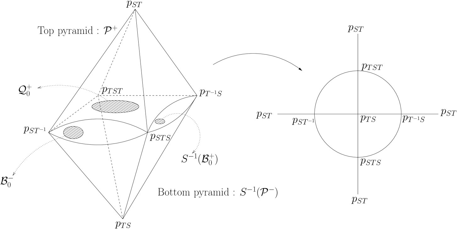
Figure 10: A combinatorial picture of the octahedron.

The faces of this octahedron are paired as follows.

$$TS : (p_{TS},p_{T^{-1}S},p_{STS})\longmapsto(p_{TS},p_{TST},p_{TS^{-1}}),$$

$$ST : (p_{ST},p_{TST},p_{T^{-1}S})\longmapsto(p_{ST},p_{ST^{-1}},p_{STS}),$$

$$T : (p_{ST},p_{TST},p_{ST^{-1}})\longmapsto(p_{TS},p_{T^{-1}S},p_{TST}),$$

$$S : (p_{TS},p_{ST^{-1}},p_{STS})\longmapsto(p_{ST},p_{STS},p_{S^{-1}T}),$$

$$S : (p_{ST^{-1}},p_{STS})\longmapsto(p_{STS},p_{S^{-1}T})$$

The last line is the bigon identification between $\mathcal{B}_{0}^{-}$ and $S^{-1}(\mathcal{B}_{0}^{+})$. As the triangle $(p_{TS},p_{ST^{-1}},p_{STS})$ and the bigon $\mathcal{B}_{0}^{-}$ share a common edge and have the same face pairing they can be combined into a single triangle, as well as their images. Thus the last two lines may be combined into a single side with side pairing map $S$. We therefore obtain a true combinatorial octahedron. The face identifications given above make the quotient manifold homeomorphic to the complement of the Whitehead link (compare for instance with Section 3.3 of [35]). ∎

7 Technicalities.

7.1 The triple intersections: proofs of Proposition 4.5 and Lemma 6.2.

In this section we first prove Proposition 4.5, which states that the triple intersection must contain a point of $\partial\mathbf{H}^{2}_{\mathbb{C}}$ and then we analyse the case of the limit group $\Gamma^{\lim}$, giving a proof of Lemma 6.2. First recall that the isometric spheres $\mathcal{I}_{0}^{-}$ and $\mathcal{I}_{-1}^{-}$ are the unit Heisenberg spheres with centres given respectively in geographical coordinates by (see 2.5)

$${\bf p}_{AB} = S(\infty)=g\bigl{(}-\alpha_{1},-\alpha_{1}/2+\alpha_{2},\sqrt{2\cos(\alpha_{1})}\bigr{)}$$

$${\bf p}_{BA} = A^{-1}S(\infty)=g\bigl{(}-\alpha_{1},-\alpha_{1}/2-\alpha_{2}+\pi,\sqrt{2\cos(\alpha_{1})}\bigr{)}.$$

Consider the two functions of points $q=g(\alpha,\beta,w)\in\mathcal{I}_{0}^{+}$ defined by

$$f^{[0]}_{\alpha_{1},\alpha_{2}}(q) = 2\cos^{2}(\alpha/2-\alpha_{1}/2)+\cos(\alpha-\alpha_{1})$$

$$\quad-4wx_{1}\cos(\alpha/2-\alpha_{1}/2)\cos(\beta+\alpha_{1}/2-\alpha_{2})+w^{2}x_{1}^{2},$$

$$f^{[-1]}_{\alpha_{1},\alpha_{2}}(q) = 2\cos^{2}(\alpha/2-\alpha_{1}/2)+\cos(\alpha-\alpha_{1})$$ (32)

$$\quad+4wx_{1}\cos(\alpha/2-\alpha_{1}/2)\cos(\beta+\alpha_{1}/2+\alpha_{2})+w^{2}x_{1}^{2}.$$

These functions characterise those points on $\mathcal{I}_{0}^{+}$ that belong to $\mathcal{I}_{0}^{-}$ and $\mathcal{I}_{-1}^{-}$.

Lemma 7.1.

A point $q$ on $\mathcal{I}_{0}^{+}$ lies on $\mathcal{I}_{0}^{-}$ (respectively in its interior or exterior) if and only if it satisfies $f^{[0]}_{\alpha_{1},\alpha_{2}}(q)=0$ (respectively is negative or is positive). Similarly, a point $q$ on $\mathcal{I}_{0}^{+}$ lies on $\mathcal{I}_{-1}^{-}$ (respectively in its interior or exterior) if and only if it satisfies $f^{[-1]}_{\alpha_{1},\alpha_{2}}(q)=0$ (respectively is negative or is positive).

Proof.

A point $q\in\mathcal{I}_{0}^{+}$ lies on $\mathcal{I}_{0}^{-}$ (respectively in its interior or exterior) if and only if its Cygan distance from the centre of $\mathcal{I}_{0}^{-}$, which is the point $p_{AB}$, equals $1$ (respectively is less than $1$ or greater than $1$). Equivalently (see Section 2.4), the following quantity vanishes, is positive or negative respectively,

$$\bigl{|}\langle{\bf q},{\bf p}_{AB}\rangle\bigr{|}^{2}-1 = \Bigl{|}-e^{-i\alpha}+wx_{1}e^{-i\alpha/2+i\beta-i\alpha_{2}}-e^{-i\alpha_{1}}\Bigr{|}^{2}-1$$

$$= \Bigl{|}-2\cos(\alpha/2-\alpha_{1}/2)+wx_{1}e^{i\beta+i\alpha_{1}/2-i\alpha_{2}}\Bigr{|}^{2}-1$$

$$= 4\cos^{2}(\alpha/2-\alpha_{1}/2)-1-4\cos(\alpha/2-\alpha_{1}/2)wx_{1}\cos(\beta+\alpha_{1}/2-\alpha/2)+w^{2}x_{1}^{2}$$

$$= f^{[0]}_{\alpha_{1},\alpha_{2}}(q).$$

On the last line we used $2\cos^{2}(\alpha/2-\alpha_{1}/2)=1+\cos(\alpha-\alpha_{1})$. This proves the first part of the Lemma and the second is obtained by a similar computation. ∎

Corollary 7.2.

For given $(\alpha_{1},\alpha_{2})$, if the sum $f^{[0]}_{\alpha_{1},\alpha_{2}}+f^{[-1]}_{\alpha_{1},\alpha_{2}}$ is positive for all $q$, then the triple intersection $\mathcal{I}_{0}^{+}\cap\mathcal{I}_{0}^{-}\cap\mathcal{I}_{-1}^{-}$ is empty.

See Figure 8. We can now prove Proposition 4.5.

Proof of Proposition 4.5..

To prove the first part, note that a necessary condition for a point $q\in\mathcal{I}_{0}^{+}$ to be in the intersection $\mathcal{I}_{0}^{-}\cap\mathcal{I}_{-1}^{-}$ is that $f_{\alpha_{1},\alpha_{2}}^{[0]}(q)-f_{\alpha_{1},\alpha_{2}}^{[-1]}(q)=0$. This difference is:

$$f^{[0]}_{\alpha_{1},\alpha_{2}}(q)-f^{[-1]}_{\alpha_{1},\alpha_{2}}(q) = -4wx_{1}\cos(\alpha/2-\alpha_{1}/2)\bigl{(}\cos(\beta+\alpha_{1}/2-\alpha_{2})+\cos(\beta+\alpha_{1}/2+\alpha_{2})\bigr{)}$$

$$= -8wx_{1}\cos(\alpha/2-\alpha_{1}/2)\cos(\beta+\alpha_{1}/2)\cos(\alpha_{2}).$$

Since $\alpha_{1}$ and $\alpha_{2}$ lie in $(-\pi/2,\pi/2)$ and $\alpha\in[-\pi/2,\pi/2]$, the only solutions are $\cos(\beta+\alpha_{1}/2)=0$ or $w=0$. Thus either $p=g(\alpha,\beta,w)$ lies on the meridian $\mathfrak{m}$, or on the spine of $\mathcal{I}_{0}^{+}$, and hence on every meridian, in particular on $\mathfrak{m}$ (compare with Proposition 2.9).

To prove the second part of Proposition 4.5, assume that the triple intersection contains a point $q=g\bigl{(}\alpha,(\pi/2-\alpha_{1}/2),w\bigr{)}$ inside $\mathbf{H}^{2}_{\mathbb{C}}$, that is such that $w^{2}<2\cos(\alpha)$, and

$$f^{[0]}_{\alpha_{1},\alpha_{2}}(q)+f^{[-1]}_{\alpha_{1},\alpha_{2}}(q)=0.$$

In view of Corollary 7.2, we only need to prove that there exists a point on $\partial\mathfrak{m}$ where the above sum is non-positive, and use the intermediate value theorem. To do so, let $\tilde{\alpha}$ be defined by the condition $2\cos(\tilde{\alpha})=w^{2}$ and such that $\tilde{\alpha}$ and $\alpha_{1}$ have opposite signs. Since $w^{2}<2\cos(\alpha)$, these conditions imply that $|\tilde{\alpha}|>|\alpha|$. We claim that the point $\tilde{q}=g\bigl{(}\tilde{\alpha},(\pi-\alpha_{1})/2,w\bigr{)}$ is satisfactory. Indeed, the conditions on $\tilde{\alpha}$ give

$$|\alpha-\alpha_{1}|\leq|\alpha|+|\alpha_{1}|<|\tilde{\alpha}|+|\alpha_{1}|=|\tilde{\alpha}-\alpha_{1}|$$

where the last inequality follows from the fact that $\tilde{\alpha}$ and $\alpha_{1}$ have opposite signs. Therefore

$$\cos(\tilde{\alpha}/2-\alpha_{1}/2)<\cos(\alpha/2-\alpha_{1}/2).$$ (33)

On the other hand, we have

$$f^{[0]}_{\alpha_{1},\alpha_{2}}(q)+f^{[-1]}_{\alpha_{1},\alpha_{2}}(q)$$ (34)

$$= 4\cos^{2}(\alpha/2-\alpha_{1}/2)+2\cos(\alpha-\alpha_{1})-8wx_{1}\cos(\alpha/2-\alpha_{1}/2)\sin(\alpha_{2})+2w^{2}x_{1}^{2}$$

$$= 8\cos^{2}(\alpha/2-\alpha_{1}/2)-2-8wx_{1}\cos(\alpha/2-\alpha_{1}/2)\sin(\alpha_{2})+2w^{2}x_{1}^{2}.$$

We claim this is an increasing function of $\cos(\alpha/2-\alpha_{1}/2)$. In order to see this, observe that its derivative with respect to this variable is

$$16\cos(\alpha/2-\alpha_{1}/2)-8wx_{1}\sin(\alpha_{2})>16\cos(\alpha/2-\alpha_{1}/2)-16\sqrt{\cos(\alpha)\cos(\alpha_{1})}\geq 0,$$

where we used $x_{1}=\sqrt{2\cos(\alpha_{1})}$, $w<\sqrt{2\cos(\alpha)}$ and $\sin(\alpha_{2})\leq 1$. Therefore,

$$0 = f^{[0]}_{\alpha_{1},\alpha_{2}}(q)+f^{[-1]}_{\alpha_{1},\alpha_{2}}(q)$$

$$= 8\cos^{2}(\alpha/2-\alpha_{1}/2)-2-8wx_{1}\cos(\alpha/2-\alpha_{1}/2)\sin(\alpha_{2})+2w^{2}x_{1}^{2}$$

$$> 8\cos^{2}(\tilde{\alpha}/2-\alpha_{1}/2)-2-8wx_{1}\cos(\tilde{\alpha}/2-\alpha_{1}/2)\sin(\alpha_{2})+2w^{2}x_{1}^{2}$$

$$= f^{[0]}_{\alpha_{1},\alpha_{2}}(\tilde{q})+f^{[-1]}_{\alpha_{1},\alpha_{2}}(\tilde{q}).$$

This proves our claim. ∎

We now prove Lemma 6.2 which completely describes the triple intersection at the limit point.

Proof of Lemma 6.2.

From the first part of Proposition 4.5 we see that any point $q=g(\alpha,\beta,w)$ in $\mathcal{I}_{0}^{+}\cap\mathcal{I}_{0}^{-}\cap\mathcal{I}_{-1}^{-}$ must lie on $\mathfrak{m}$, that is $\beta=(\pi-\alpha_{1})/2$. For such points it is enough to show that $f^{[0]}_{0,\alpha_{2}^{\lim}}(q)+f^{[-1]}_{0,\alpha_{2}^{\lim}}(q)=0$. Substituting $\alpha_{1}=0$ and $\sin(\alpha_{2})=\sqrt{5/8}$, this becomes:

$$f^{[0]}_{0,\alpha_{2}^{\lim}}(q)+f^{[-1]}_{0,\alpha_{2}^{\lim}}(q) = 4\cos^{2}(\alpha/2)+\cos(\alpha)-4\sqrt{5}w\cos(\alpha/2)+4w^{2}$$

$$= \Bigl{(}2\cos(\alpha/2)-\sqrt{5}w\Bigr{)}^{2}+\bigl{(}2\cos(\alpha)-w^{2}\bigr{)}.$$

In order to vanish, both terms must be zero. Hence $w^{2}=2\cos(\alpha)$ and $2\cos(\alpha/2)=\sqrt{5}w=\sqrt{10\cos(\alpha)}$ (noting $w$ cannot be negative since $\alpha\in[-\pi/2,\pi/2]$). This means $\alpha=\pm\arccos(1/4)$ and $w=\sqrt{2\cos(\alpha)}=1/\sqrt{2}$. Therefore, the only points in $\mathcal{I}_{0}^{+}\cap\mathcal{I}_{0}^{-}\cap\mathcal{I}_{-1}^{-}$ have geographical coordinates $g\bigl{(}\pm\arccos(1/4),\pi/2,1/\sqrt{2}\bigr{)}$. Using (6.1), we see these points are $p_{ST^{-1}}$ and $p_{S^{-1}T}$. ∎

7.2 The region $\mathcal{Z}$ is an open disc in the region $\mathcal{L}$: Proof of Proposition 4.4.

Consider the group $\Gamma_{\alpha_{1},\alpha_{2}}$ and, as before, write $x_{1}^{4}=4\cos^{2}(\alpha_{1})$ and $x_{2}^{4}=4\cos^{2}(\alpha_{2})$. Recall, from Proposition 3.7, that $(\alpha_{1},\alpha_{2})$ is in ${\mathcal{L}}$ (respectively ${\mathcal{P}}$) if $\mathcal{G}(x_{1}^{4},x_{2}^{4})>0$ (respectively $=0$) where:

$$\mathcal{G}(x,y)=x^{2}y^{4}-4x^{2}y^{3}+18xy^{2}-27.$$ (35)

Recall this means $[A,B]$ is loxodromic (respectively parabolic). Also $(\alpha_{1},\alpha_{2})$ is in the rectangle $\mathcal{R}$ if and only if $(x_{1}^{4},x_{2}^{4})\in[3,4]\times[3/2,4]$. From Proposition 4.3, the point $(\alpha_{1},\alpha_{2})\in\mathcal{R}$ is in $\mathcal{Z}$ (respectively $\partial\mathcal{Z}$) if $\mathcal{D}(x_{1}^{4},x_{2}^{4})>0$ (respectively $=0$) where:

$$\mathcal{D}(x,y)=x^{3}y^{3}-9x^{2}y^{2}-27xy^{2}+81xy-27x-27.$$ (36)

Lemma 7.3.

Suppose $(\alpha_{1},\alpha_{2})\in\mathcal{R}$. Then $(\alpha_{1},\alpha_{2})\in{\mathcal{L}}\cup\mathcal{P}$, that is the commutator $[A,B]$ is loxodromic or parabolic (see Section 3.4). Moreover, $(\alpha_{1},\alpha_{2})\in\mathcal{P}$ if and only if $(\alpha_{1},\alpha_{2})=(0,\pm\alpha_{2}^{\lim})$.

Proof.

We first claim that the function $\mathcal{G}(x,y)$ has no critical points in $(0,\infty)\times(0,\infty)$. Indeed, the first partial derivatives of $\mathcal{G}(x,y)$ are

$$\mathcal{G}_{x}(x,y)=2y^{2}(xy^{2}-4xy+9),\quad\mathcal{G}_{y}(x,y)=4xy(xy^{2}-3xy+9).$$

These are not simultaneously zero for any positive values of $x$ and $y$. As a consequence, the minimum of $\mathcal{G}$ on $[3,4]\times[3/2,4]$ is attained on the boundary of this rectangle. We then have:

$$\begin{array}[]{ll}\mathcal{G}(x,3/2)=\dfrac{27}{16}\left(4-x\right)\left(5x-4\right),&\mathcal{G}(x,4)=9(32x-3),\\ \mathcal{G}(3,y)=9\left(y-1\right)\left(y^{3}-3y^{2}+3y+3\right),&\mathcal{G}(4,y)=(2y+1)(2y-3)^{3}.\end{array}$$

It is a simple exercise to check that under the assumptions that $3\leq x\leq 4$ and $3/2\leq y\leq 4$ all four of these terms are positive, except for when $(x,y)=(4,3/2)$ in which case $\mathcal{G}(4,3/2)=0$. Then $(x_{1}^{4},x_{2}^{4})=(4,3/2)$ if and only if $(\alpha_{1},\alpha_{2})=(0,\pm\alpha_{2}^{\lim})$; compare to Figure 4. ∎

Figure 11: The null locus of $\mathcal{D}(x,y)$ in the rectangle $[3,4]\times[3/2,4]$.

Lemma 7.4.

The region $\mathcal{Z}$ is an open topological disc in $\mathcal{R}$ symmetric about the axes and intersecting them in the intervals $\{\alpha_{2}=0,\,-\pi/6<\alpha_{1}<\pi/6\}$ and $\{\alpha_{1}=0,\,-\alpha_{2}^{\lim}<\alpha_{2}<\alpha_{2}^{\lim}\}$. Moreover, the only points of $\partial\mathcal{Z}$ that lie in the boundary of $\mathcal{R}$ are $(\alpha_{1},\alpha_{2})=(0,\pm\alpha_{2}^{\lim})$ and $(\alpha_{1},\alpha_{2})=(\pm\pi/6,0)$.

Proof.

First we examine the values of $\mathcal{D}(x,y)$ on the boundary of $[3,4]\times[3/2,4]$:

$$\begin{array}[]{ll}\mathcal{D}\left(x,3/2\right)=\frac{27}{8}(x-4)(x^{2}-2x+2),&\mathcal{D}(x,4)=(x-3)(3+8x)^{2},\\ \mathcal{D}(3,y)=27(y-4)(y-1)^{2},&\mathcal{D}(4,y)=(16y-15)(2y-3)^{2}.\end{array}$$ (37)

We claim that, for any $y_{0}\in[3/2,4]$ the polynomial $\mathcal{D}(x,y_{0})$ has exactly one root in $[3,4]$. Indeed, we have $\mathcal{D}(3,y_{0})\leq 0\leq\mathcal{D}(4,y_{0})$ and thus $\mathcal{D}(x,y_{0})$ has at least one such root. The $x$-derivative of $\mathcal{D}$ is

$$\partial_{x}\mathcal{D}(x,y)=3(x-3)y^{2}(xy+3y-6)+27(y-1)^{3},$$

which is positive when $x\in[3,4]$ and $y\in[3/2,4]$. Thus $\mathcal{D}(x,y_{0})$ is increasing, and the root is unique.

Similarly, we claim that, for any $x_{0}\in[3,4]$, the polynomial $\mathcal{D}(x_{0},y)$ has a unique root in $[3/2,4]$. It is clear from (37) when $x_{0}=4$ (there the root is $y=3/2$). Now suppose $3\leq x_{0}<4$. Arguing as before, we have $\mathcal{D}(x_{0},3/2)<0\leq\mathcal{D}(x_{0},4)$. However, it is not true that $\mathcal{D}(x_{0},y)$ is a monotone function of $y$. The partial derivative of $\mathcal{D}(x,y)$ with respect to $y$ is

$$\partial_{y}\mathcal{D}(x,y)=3x(x^{2}y^{2}-6xy-18y+27).$$

Therefore, for a fixed $x_{0}\in[3,4)$ we have $\partial_{y}\mathcal{D}(x_{0},3/2)=27x_{0}^{2}(x_{0}-4)/4<0$. Since $\mathcal{D}(x_{0},y)$ is a cubic with leading coefficient $x_{0}^{3}>0$, such that both $\mathcal{D}(x_{0},3/2)$ and $\partial_{y}\mathcal{D}(x_{0},3/2)$ are negative we see that $\mathcal{D}(x_{0},y)$ has exactly one zero in $(3/2,\infty)$. Since $\mathcal{D}(x_{0},4)\geq 0$ this zero must lies in $(3/2,4]$ as claimed.

Thus the zero-locus of $\mathcal{D}(x,y)$ in $[3,4]\times[3/2,4]$ is the graph of a continuous bijection connecting the two points $(3,4)$ and $(4,3/2)$. The polynomial $\mathcal{D}(x,y)$ is positive in the part of $[3,4]\times[3/2,4]$ above the zero-locus, that is containing the point $(x,y)=(4,4)$ (see Figure 11). Likewise, it is negative in the part below the zero locus, that is containing the point $(x,y)=(3,3/2)$. Changing coordinates to $(\alpha_{1},\alpha_{2})$, we see that the zero locus of $\mathcal{D}\bigl{(}4\cos^{2}(\alpha_{1}),4\cos^{2}(\alpha_{2})\bigr{)}$ in the rectangle $[0,\pi/6]\times[0,\alpha_{2}^{\lim}]$ is the graph of a continuous bijection connecting the points $(\alpha_{1},\alpha_{2})=(\pi/6,0)$ and $(0,\alpha_{2}^{\lim})$. Moreover, $\mathcal{D}$ is positive on the part below this curve, in particular on the interval $\alpha_{1}=0$ and $0\leq\alpha_{2}<\alpha_{2}^{\lim}$ and the interval $\alpha_{2}=0$ and $0\leq\alpha_{1}<\pi/6$. The region $\mathcal{Z}$ is the union of the four copies of this region by the symmetries about the horizontal and vertical coordinate axes. It is clearly a disc and contains the relevant parts of the axes. This completes the proof. ∎

Combining Lemmas 7.3 and 7.4 proves Proposition 4.4.

7.3 Condition for no triple intersections: Proof of Proposition 4.3.

In this section we find a condition on $(\alpha_{1},\alpha_{2})$ that characterises the set $\mathcal{Z}$ where the triple intersection of isometric spheres $\mathcal{I}_{0}^{+}\cap\mathcal{I}_{0}^{-}\cap\mathcal{I}_{-1}^{-}$ is empty.

Lemma 7.5.

The triple intersection $\mathcal{I}_{0}^{+}\cap\mathcal{I}_{0}^{-}\cap\mathcal{I}_{-1}^{-}$ is empty if and only if $f_{\alpha_{1},\alpha_{2}}(\alpha)>0$ for all $\alpha\in[-\pi/2,\pi/2]$ where

$$f_{\alpha_{1},\alpha_{2}}(\alpha) = 4\cos^{2}(\alpha/2-\alpha_{1}/2)+2\cos(\alpha-\alpha_{1})+8\cos(\alpha)\cos(\alpha_{1})$$

$$\quad-16\sqrt{\cos(\alpha)\cos(\alpha_{1})}\cos(\alpha/2-\alpha_{1}/2)\bigl{|}\sin(\alpha_{2})\bigr{|}.$$

Proof.

By Corollary 7.2, it is enough to show that $f^{[0]}_{\alpha_{1},\alpha_{2}}+f^{[-1]}_{\alpha_{1},\alpha_{2}}>0$. This sum is made explicit in (34). In view of the second part of Proposition (4.5), we can restrict our attention to showing that the triple intersection $\mathcal{I}_{0}^{+}\cap\mathcal{I}_{0}^{-}\cap\mathcal{I}_{-1}^{-}$ contains no points of $\partial\mathbf{H}^{2}_{\mathbb{C}}$. That is, we may assume $w=\pm\sqrt{2\cos(\alpha)}$. Using the first part of Proposition 4.5 we restrict our attention to points $m$ in the meridian $\mathfrak{m}$ where $\beta=(\pi-\alpha_{1})/2$. The triple intersection is empty if and only if the sum $f^{[0]}_{\alpha_{1},\alpha_{2}}(q)+f^{[-1]}_{\alpha_{1},\alpha_{2}}(q)$ is positive for any value of $\alpha$, where $q=g\bigl{(}\alpha,(\pi-\alpha_{1}/2),\pm\sqrt{2\cos(\alpha)}\bigr{)}$. When $w\sin(\alpha_{2})$ is negative all terms in (34) are positive. Therefore we may suppose $w\sin(\alpha_{2})=\sqrt{2\cos(\alpha_{1})}\bigl{|}\sin(\alpha_{2})\bigr{|}\geq 0$. Substituting these values in the expression for $f^{[0]}_{\alpha_{1},\alpha_{2}}(q)+f^{[-1]}_{\alpha_{1},\alpha_{2}}(q)$ given in (34) gives the function $f_{\alpha_{1},\alpha_{2}}(\alpha)$ in (7.5). ∎

We want to convert (7.5) into a polynomial expression in a function of $\alpha$. The numerical condition given in the statement of Proposition 4.3 will follow from the next lemma.

Lemma 7.6.

If $\alpha\in[-\pi/2,\pi/2]$ is a zero of $f_{\alpha_{1},\alpha_{2}}$ then $T_{\alpha}=\tan(\alpha/2)\in[-1,1]$ is a root of the quartic polynomial $L_{\alpha_{1},\alpha_{2}}(T)$, where

$$L_{\alpha_{1},\alpha_{2}}(T) = T^{4}\left(2x_{1}^{4}x_{2}^{4}-4x_{1}^{2}x_{2}^{4}+x_{1}^{4}+10x_{1}^{2}+1\right)-8T^{3}\sin(\alpha_{1})\left(x_{1}^{2}x_{2}^{4}-x_{1}^{2}-1\right)$$ (39)

$$-2T^{2}\left(2x_{1}^{4}x_{2}^{4}+3x_{1}^{4}-9\right)+8T\sin(\alpha_{1})\left(x_{1}^{2}x_{2}^{4}-x_{1}^{2}+1\right)$$

$$+\left(2x_{1}^{4}x_{2}^{4}+4x_{1}^{2}x_{2}^{4}+x_{1}^{4}-10x_{1}^{2}+1\right)$$

Proof.

Squaring the two lines of (7.5) and using $\sqrt{2\cos(\alpha_{1})}\bigl{|}\sin(\alpha_{2})\bigr{|}\geq 0$, we see that the condition $f_{\alpha_{1},\alpha_{2}}(\alpha)=0$ is equivalent to

$$\Bigl{(}2\cos^{2}(\alpha/2-\alpha_{1}/2)+\cos(\alpha-\alpha_{1})+4\cos(\alpha)\cos(\alpha_{1})\Bigr{)}^{2}=64\cos(\alpha)\cos(\alpha_{1})\cos^{2}(\alpha/2-\alpha_{1}/2)\sin^{2}(\alpha_{2}).\\$$

After rearranging and expanding, we obtain the following polynomial equation in $\cos(\alpha)$ and $\sin(\alpha)$.

$$0 = 4\left(8\cos^{2}(\alpha_{1})\cos^{2}(\alpha_{2})+2\cos^{2}(\alpha_{1})-1\right)\cos^{2}(\alpha)+4\cos(\alpha_{1})\bigl{(}8\cos^{2}(\alpha_{2})-5\bigr{)}\cos(\alpha)$$

$$\quad+8\cos(\alpha_{1})\sin(\alpha_{1})\left(4\cos^{2}(\alpha_{2})-1\right)\cos(\alpha)\sin(\alpha)+4\sin(\alpha_{1})\sin(\alpha)-4\cos^{2}(\alpha_{1})+5.$$

Substituting $\tan(\alpha/2)=T$, $2\cos(\alpha_{1})=x_{1}^{2}$ and $2\cos(\alpha_{2})=x_{2}^{2}$ into this equation gives $L_{\alpha_{1},\alpha_{2}}(T)$. ∎

Before proving Proposition 4.3, we analyse the situation on the axes $\alpha_{1}=0$ and $\alpha_{2}=0$.

Lemma 7.7.

Let $L_{\alpha_{1},\alpha_{2}}(T)$ be given by (39).

1. When $\alpha_{2}=0$ and $-\pi/6<\alpha_{1}<\pi/6$ then $L_{\alpha_{1},0}(T)$ has two real double roots $T_{-}$ and $T_{+}$ where $T_{-}<-1$ and $T_{+}>1$, and no other roots.

2. When $\alpha_{1}=0$ and $0<\alpha_{2}<\alpha_{2}^{\lim}$ or $-\alpha_{2}^{\lim}<\alpha_{2}<0$ the polynomial $L_{0,\alpha_{2}}(T)$ has no real roots.

Proof.

First, substituting $\alpha_{2}=0$ in (39) we find $L_{(\alpha_{1},0)}=M_{\alpha_{1}}(T)^{2}$, where

$$M_{\alpha_{1}}(T)=T^{2}(3x_{1}^{2}-1)-4T\sin(\alpha_{1})-(3x_{1}^{2}+1).$$

The condition on $\alpha_{1}$ guarantees that $3x_{1}^{2}-1>0$ and so as $T$ tends to $\pm\infty$ so $M_{\alpha_{1}}(T)$ tends to $+\infty$. On the other hand,

$$M_{\alpha_{1}}(-1)=4\sin(\alpha_{1})-2<0,\quad M_{\alpha_{1}}(1)=-4\sin(\alpha_{1})-2<0.$$

Therefore $M_{\alpha_{1}}(T)$ has two real roots $T_{-}<-1$ and $T_{+}>1$ as claimed. Since $M_{\alpha_{1}}(T)$ is quadratic, it cannot have any more roots. In particular, it is negative for $-1\leq T\leq 1$.

Secondly, we substitute $\alpha_{1}=0$ in (39), giving:

$$L_{0,\alpha_{2}}(T)=\left(5T^{2}-\frac{8x_{2}^{4}+3}{5}\right)^{2}+\frac{32}{25}(2x_{2}^{4}-3)(4-x_{2}^{4}).$$

When $\alpha_{2}\in(-\alpha_{2}^{\lim},\alpha_{2}^{\lim})$ and $\alpha_{2}\neq 0$, we have $x_{2}^{4}=4\cos^{2}(\alpha_{2})\in(3/2,4)$. In particular, this means that $(2x_{2}^{4}-3)(4-x_{2}^{4})>0$ and so $L_{0,\alpha_{2}}(T)$ has no real roots, proving the second part. ∎

We note that when $\alpha_{1}=\alpha_{2}=0$ then $L_{0,0}(T)$ has double roots at $T=\pm\sqrt{7/5}$ and when $\alpha_{1}=0$ and $\alpha_{2}=\pm\alpha_{2}^{\lim}$ then $L_{0,\pm\alpha_{2}^{\lim}}(T)$ has double roots at $T=\pm\sqrt{3/5}$.

Lemma 7.8.

If $(\alpha_{1},\alpha_{2})\in\mathcal{Z}$ then the polynomial $L_{\alpha_{1},\alpha_{2}}(T)$ has no roots $T$ in $[-1,1]$.

Proof.

We analyse the number, type (real or non-real) and location of roots of the polynomial $L_{\alpha_{1},\alpha_{2}}(T)$ when $(\alpha_{1},\alpha_{2})\in\mathcal{R}$. As $L_{\alpha_{1}\alpha_{2}}(T)$ has real coefficients, whenever it has only simple roots, its root set is of one of the following types:

1. two pairs of complex conjugate non real simple roots,

2. a pair of non-real complex conjugate simple roots and two simple real roots,

3. four simple real roots.

But the set of roots of a polynomial is a continuous map (in bounded degree) for the Hausdorff distance on compact subsets of $\mathbb{C}$. In particular, the root set type of $L_{\alpha_{1},\alpha_{2}}(T)$ is a continuous function of $\alpha_{1}$ and $\alpha_{2}$. This implies that it is not possible to pass from one of the above types to another without passing through a polynomial having a double root.

We compute the discriminant $\Delta_{\alpha_{1},\alpha_{2}}$ of $L_{\alpha_{1},\alpha_{2}}(T)$ (a computer may be useful to do so):

$$\Delta_{\alpha_{1},\alpha_{2}} = 2^{16}x_{1}^{4}\bigl{(}x_{1}^{4}+1\bigr{)}^{2}\bigl{(}2x_{1}^{2}(2-x_{1}^{2})(4-x_{2}^{4})+(3x_{1}^{2}-1)^{2}\bigr{)}\bigl{(}4-x_{2}^{4}\bigr{)}^{2}\cdot\mathcal{D}\bigl{(}x_{1}^{4},x_{2}^{4}\bigr{)}$$ (40)

where $\mathcal{D}(x,y)$ is as in Proposition 4.3, and $x_{i}=\sqrt{2\cos(\alpha_{i})}$. The polynomial $L_{\alpha_{1},\alpha_{2}}(T)$ has a multiple root in $\mathbb{C}$ if and only if $\Delta_{\alpha_{1}\alpha_{2}}=0$. Let us examine the different factors.

• The first two factors $x_{1}^{4}$ and $(x_{1}^{4}+1)^{2}$ are positive when $(\alpha_{1},\alpha_{2})\in(-\pi/2,\pi/2)^{2}$.

• Note that $(2-x_{1}^{2})(4-x_{2}^{4})\geq 0$ and $(3x_{1}^{2}-1)^{2}>0$ when $\sqrt{3}\leq x_{1}^{2}\leq 2$ and $x_{2}^{4}\leq 4$, and so the third factor is positive.

Thus, the only factors of $\Delta_{\alpha_{1},\alpha_{2}}$ that can vanish on $\mathcal{R}$ are $(4-x_{2}^{4})^{2}=16\sin^{4}\alpha_{2}$ and $\mathcal{D}(x_{1}^{4},x_{2}^{4})$. In particular $L_{\alpha_{1},\alpha_{2}}(T)$ has a multiple root in $\mathbb{C}$ if and only if one of these two factors vanishes. We saw in Proposition 4.4 that the subset of $\mathcal{R}$ where $\mathcal{D}(x_{1}^{4},x_{2}^{4})>0$ is a topological disc $\mathcal{Z}$, symmetric about the $\alpha_{1}$ and $\alpha_{2}$ axes and intersecting them in the intervals $\{\alpha_{2}=0,\,-\pi/6<\alpha_{1}<\pi/6\}$ and $\{\alpha_{1}=0,\,-\alpha_{2}^{\lim}<\alpha_{2}<\alpha_{2}^{\lim}\}$. Therefore, the rectangle $\mathcal{R}$ contains two open discs on which $\Delta_{\alpha_{1},\alpha_{2}}>0$, namely

$$\mathcal{Z}^{+}=\{(\alpha_{1},\alpha_{2})\in\mathcal{Z}\ :\ \alpha_{2}>0\},\quad\mathcal{Z}^{-}=\{(\alpha_{1},\alpha_{2})\in\mathcal{Z}\ :\ \alpha_{2}<0\}.$$

These two sets each contain an open interval of the $\alpha_{2}$ axis. We saw in the second part of Lemma 7.7 that on both these intervals $L_{\alpha_{1},\alpha_{2}}(T)$ has no real roots, that is its roots are of type (a). Therefore it has no real roots on all of $\mathcal{Z}^{+}$ and $\mathcal{Z}^{-}$.

The only points of $\mathcal{Z}$ yet to be considered are those in the interval $\{\alpha_{2}=0,\,-\pi/6<\alpha_{1}<\pi/6\}$. We saw in the first part of Lemma 7.7 that for such points $L_{\alpha_{1},\alpha_{2}}(T)$ has no roots with $-1\leq T\leq 1$. This completes the proof of Proposition 4.3. ∎

7.4 Pairwise intersection: Proof of Proposition 4.6.

Proposition 4.6 will follow from the next lemma.

Lemma 7.9.

If $0<x\leq 4$ and $\mathcal{D}(x,y)\geq 0$ then $xy\geq 6$ with equality if and only if $(x,y)=(4,3/2)$.

Proof.

Substituting $y=6/x$ in (36) and simplifying, we find $\mathcal{D}(x,6/x)=-27(x-4)(x-9)/x$. When $0<x\leq 4$ we see immediately that this is non-positive and equals zero if and only if $x=4$. This means that $xy-6$ has a constant sign on the region where $\mathcal{D}(x,y)>0$. Checking at $(x,y)=(4,4)$ we see that it is positive. ∎

Proof of Proposition 4.6.

To prove the disjointness of the given isometric spheres we calculate the Cygan distance between their centres. Since all the isometric spheres have radius $1$, if we can show their centres are a Cygan distance at least $2$ apart, then the spheres are disjoint. (Note that the Cygan distance is not a path metric, so it may be the distance is less than $2$ but the spheres are still disjoint. This will not be the case in our examples.)

The centre of $I_{k}^{+}$ is $A^{k}(p_{B})=\bigl{[}kx_{1}x_{2}^{2}/\sqrt{2},kx_{1}^{2}x_{2}^{2}\sin(\alpha_{2})\bigr{]}$; see Proposition 4.1. We will show that $d_{\rm Cyg}\bigl{(}A^{k}(p_{B}),p_{B}\bigr{)}^{4}>16$ when $k^{2}\geq 4$ and $(\alpha_{1},\alpha_{2})\in\mathcal{R}$, that is $(x_{1}^{4},x_{2}^{4})\in[3,4]\times[3/2,4]$:

$$d_{\rm Cyg}\bigl{(}A^{k}(p_{B}),p_{B}\bigr{)}^{4} = \frac{k^{4}x_{1}^{4}x_{2}^{8}+k^{2}x_{1}^{4}x_{2}^{4}(4-x_{2}^{4})}{4}$$

$$\geq \frac{27k^{4}}{16}.$$

This number is greater than $16$ when $k\geq 2$ or $k\leq-2$ as claimed.

Again using Proposition 4.1, the centre of $\mathcal{I}_{k}^{-}$ is $A^{k}(p_{AB})=\bigl{[}(kx_{1}x_{2}^{2}+x_{1}e^{i\alpha_{2}})/\sqrt{2},-\sin(\alpha_{1})\bigr{]}$. We suppose $(x_{1}^{4},x_{2}^{4})\in[3,4]\times[3/2,4]$ satisfies $x_{1}^{4}x_{2}^{4}\geq 6$, which is valid for $(\alpha_{1},\alpha_{2})\in{\mathcal{Z}}$ by Lemma 7.9.

$$d_{\rm Cyg}\bigl{(}A^{k}(p_{AB}),p_{B}\bigr{)}^{4} = \frac{\bigl{(}k(k+1)x_{1}^{2}x_{2}^{4}+x_{1}^{2}\bigr{)}^{2}+4-x_{1}^{4}}{4}$$

$$= 1+\frac{k^{2}(k+1)^{2}x_{1}^{4}x_{2}^{8}+2k(k+1)x_{1}^{4}x_{2}^{4}}{4}$$

$$\geq \left(\frac{3k(k+1)}{2}+1\right)^{2}.$$

This number is at least $16$ when $k\geq 1$ or $k\leq-2$ as claimed. Moreover, we have equality exactly when $k=1$ or $k=-2$ and when $x_{1}^{4}x_{2}^{4}=6$ and $x_{2}^{4}=3/2$; that is when $(x_{1}^{4},x_{2}^{4})=(4,3/2)$. ∎

7.5 $\partial_{\infty}D$ is a cylinder: Proof of Proposition 6.8.

To prove Proposition 6.8, we adopt the following strategy.

• Step 1. First, we intersect $D$ with a fundamental domain $D_{A}$ for the action of $A$ on the Heisenberg group. The domain $D_{A}$ is bounded by two parallel vertical planes $F_{-1}$ and $F_{0}$ that are boundaries of fans in the sense of [17]. These two fans are such that $A(F_{-1})=F_{0}$ (see Figure 7 for a view of the situation in vertical projection). We analyse the intersections of $F_{0}$ and $F_{-1}$ with $D$, and show that they are topological circles, denoted by $c_{-1}$ and $c_{0}$ with $A(c_{-1})=c_{0}$.

• Step 2. Secondly, we consider the subset of the complement of $D$ which is contained in $D_{A}$, and prove that it is a 3-dimensional ball that intersects $F_{-1}$ and $F_{0}$ along topological discs (bounded by $c_{-1}$ and $c_{0}$). This proves that $D\cap D_{A}$ is the complement a solid tube in $D_{A}$, which is unknotted using Lemma 6.7. Finally, we prove that, gluing together copies by powers of $A$ of $D\cap D_{A}$, we indeed obtain the complement of a solid cylinder.

We construct a fundamental domain $D_{A}$ for the cyclic group of Heisenberg translations $\langle A\rangle$. The domain $D_{A}$ will be bounded by two fans, chosen to intersect as few bisectors as possible. The fan $F_{0}$ will pass through $p_{ST^{-1}}$ and will be tangent to both $\mathcal{I}_{1}^{+}$ and $\mathcal{I}_{-1}^{-}$; compare Figure 7. Similarly, $F_{-1}=A^{-1}(F_{0})$ will pass through $A^{-1}(p_{ST^{-1}})=p_{TST}$ and be tangent to both $\mathcal{I}_{0}^{+}$ and $\mathcal{I}_{-2}^{-}$. We first give $F_{0}$ and $F_{-1}$ in terms of horospherical coordinates and then we give them in terms of their own geographical coordinates (see [17]). In horospherical coordinates they are:

$$F_{0} = \Bigl{\{}[x+iy,t]\ :\ 3x\sqrt{3}-y\sqrt{5}=\sqrt{2}/2\Bigr{\}},$$ (41)

$$F_{-1} = \Bigl{\{}[x+iy,t]\ :\ 3x\sqrt{3}-y\sqrt{5}=-4\sqrt{2}\Bigr{\}}.$$ (42)

This leads to the definition of $D_{A}$:

$$D_{A}=\Bigl{\{}[x+iy,t]\ :\ -4\sqrt{2}\leq 3x\sqrt{3}-y\sqrt{5}\leq\sqrt{2}/2\Bigr{\}}.$$ (43)

We choose geographical coordinates $(\xi,\eta)$ on $F_{0}$: the lines where $\xi$ is constant (respectively $\eta$ is constant) are boundaries of complex lines (respectively Lagrangian planes). These coordinates correspond to the double foliation of fans by real planes and complex lines, which is described in Section 5.2 of [17]. The particular choice is made so that the origin is the midpoint of the centres of $\mathcal{I}_{0}^{+}$ and $\mathcal{I}_{0}^{-}$. Doing so gives the fan $F_{0}$ as the set of points $f(\xi,\eta)$:

$$f(\xi,\eta)=\left\{\left[\frac{\sqrt{5}\xi+\sqrt{3}+3i\sqrt{3}\xi+i\sqrt{5}}{4\sqrt{2}},\ \eta-\xi/4\right]\ :\ \xi,\,\eta\in{\mathbb{R}}\right\}.$$

The standard lift of $f(\xi,\eta)$ is given by

$${\bf f}(\xi,\eta)=\left[\begin{matrix}-\xi^{2}-\sqrt{15}\xi/4-1/4+i\eta-i\xi/4\\ \sqrt{5}\xi/4+\sqrt{3}/4+3i\sqrt{3}\xi/4+i\sqrt{5}/4\\ 1\end{matrix}\right].$$

Using the convexity of Cygan spheres, we see that their intersection with $F_{0}$ (or $F_{-1}$) is one of: empty, a point or a topological circle. For the particular fans and isometric spheres of interest to us, the possible intersections are summarised in the following result:

Proposition 7.10.

The intersections of the fans $F_{-1}$ and $F_{0}$ with the isometric spheres $\mathcal{I}_{k}^{\pm}$ are empty, except for those indicated in the following table.

$$\begin{array}[]{|c|c|c|c|c|c|c|c|c|}\hline\cr\bigcap&\mathcal{I}_{-2}^{-}&\mathcal{I}_{-2}^{+}&\mathcal{I}_{-1}^{-}&\mathcal{I}_{-1}^{+}&\mathcal{I}_{0}^{-}&\mathcal{I}_{0}^{+}&\mathcal{I}_{1}^{-}&\mathcal{I}_{1}^{+}\\ \hline\cr F_{0}&\emptyset&\emptyset&\{p_{ST^{-1}}\}&\emptyset&\hbox{a circle}&\hbox{a circle}&\emptyset&\{p_{ST^{-1}}\}\\ F_{-1}&\{{p_{TST}\}}&\emptyset&\hbox{a circle}&\hbox{a circle}&\emptyset&\{{p_{TST}\}}&\emptyset&\emptyset\\ \hline\cr\end{array}$$

Moreover, the point $p_{S^{-1}T}$ belongs to the interior of $D_{A}$. The parabolic fixed points $A^{k}(p_{ST^{-1}})$ lie outside $D_{A}$ for all $k\geq 1$ and $k\leq-1$; parabolic fixed points $A^{k}(p_{S^{-1}T})$ lie outside $D_{A}$ for all $k\neq 0$.

A direct consequence of this proposition is that the only point in the closure of the quadrilateral $\mathcal{Q}_{-1}^{-}$ and the bigon $\mathcal{B}_{-1}^{-}$ that lie on $F_{0}$ is their vertex $p_{TST}$.

Proof.

The part about intersections of fans and isometric spheres is proved easily by projecting vertically onto $\mathbb{C}$, as in the proof of Proposition 4.6 (see Figure 7). Note that as isometric spheres are strictly convex, their intersections with a plane is either empty or a point or a topological circle. The part about the parabolic fixed points is a direct verification using (41) as well as (6.1). ∎

We need to be slightly more precise about the intersection of $F_{0}$ with $\mathcal{I}_{0}^{+}$ and $\mathcal{I}_{0}^{-}$.

Proposition 7.11.

The intersection of $F_{0}$ with $\mathcal{I}_{0}^{+}\cup\mathcal{I}_{0}^{-}$ (and thus with $\partial D$) is a topological circle $c_{0}$, which is the union of two topological segments $c_{0}^{+}$ and $c_{0}^{-}$, where the segment $c_{0}^{\pm}$ is the part of $F_{0}\cap\mathcal{I}_{0}^{\pm}$ that is outside $\mathcal{I}_{0}^{\mp}$. The two segments $c_{0}^{+}$ and $c_{0}^{-}$ have the same endpoints: one of them is $p_{ST^{-1}}$, and we will denote the other by $q_{0}$. Moreover, the point $q_{0}$ lies on the segment $[p_{STS},p_{S^{-1}T}]$ of $\mathcal{I}_{0}^{+}\cap\mathcal{I}_{0}^{-}$.

The point $q_{0}$ appears in Figures 12, 14 and 14.

Proof.

The point $f(\xi,\eta)$ of the fan $F_{0}$ lies of $\mathcal{I}_{0}^{+}$ whenever $1=\bigl{|}\langle{\bf f}(\xi,\eta),{\bf p}_{B}\rangle\bigr{|}$ and on $\mathcal{I}_{0}^{-}$ whenever $1=\bigl{|}\langle{\bf f}(\xi,\eta),{\bf p}_{AB}\rangle\bigr{|}$. We first find all points on $F_{0}\cap\mathcal{I}_{0}^{+}\cap\mathcal{I}_{0}^{-}$. These correspond to simultaneous solutions to:

$$1=\bigl{|}\langle{\bf f}(\xi,\eta),{\bf p}_{B}\rangle\bigr{|}=\bigl{|}\langle{\bf f}(\xi,\eta),{\bf p}_{AB}\rangle\bigr{|}$$ (44)

Computing these products and rearranging, we obtain

$$\bigl{|}\langle{\bf f}(\xi,\eta),{\bf p}_{B}\rangle\bigr{|}^{2} = (\xi^{2}+1/4)^{2}+\xi^{2}+\eta^{2}+\xi\Bigl{(}\sqrt{15}\xi^{2}+\sqrt{15}/4-\eta\Bigr{)}/2,$$

$$\bigl{|}\langle{\bf f}(\xi,\eta),{\bf p}_{AB}\rangle\bigr{|}^{2} = (\xi^{2}+1/4)^{2}+\xi^{2}+\eta^{2}-\xi\Bigl{(}\sqrt{15}\xi^{2}+\sqrt{15}/4-\eta\Bigr{)}/2.$$

Subtracting, we see that solutions to (44) must either have $\xi=0$ or $\eta=\sqrt{15}(\xi^{2}+1/4)$. Substituting these solutions into $1=\bigl{|}\langle{\bf f}(\xi,\eta),{\bf p}_{B}\rangle\bigr{|}^{2}$, we see first that $\xi=0$ implies $1=\eta^{2}+1/16$; and secondly that $\eta=\sqrt{15}(\xi^{2}+1/4)$ implies

$$1=(\xi^{2}+1/4)^{2}+\xi^{2}+15(\xi^{2}+1/4)^{2}=(4\xi^{2}+1)^{2}+\xi^{2}.$$

Clearly the only solution to this equation is $\xi=0$. So both cases lead to the solutions $(\xi,\eta)=(0,\pm\sqrt{15}/4)$. Thus the only points satisfying (44), that is the points in $F_{0}\cap\mathcal{I}_{0}^{+}\cap\mathcal{I}_{0}^{-}$, are

$$f(0,\sqrt{15}/4)=\left[\frac{\sqrt{3}+i\sqrt{5}}{4\sqrt{2}},\ \frac{\sqrt{15}}{4}\right]\mbox{ and }f(0,-\sqrt{15}/4)=\left[\frac{\sqrt{3}+i\sqrt{5}}{4\sqrt{2}},\ \frac{-\sqrt{15}}{4}\right].$$

Note that the first of these points is $p_{ST^{-1}}$. We call the other point $q_{0}$.

These two points divide $F_{0}\cap\mathcal{I}_{0}^{+}$ and $F_{0}\cap\mathcal{I}_{0}^{-}$ into two arcs. It remains to decide which of these arcs is outside the other isometric sphere. Clearly $\bigl{|}\langle{\bf f}(\xi,\eta),{\bf p}_{B}\rangle\bigr{|}>\bigl{|}\langle{\bf f}(\xi,\eta),{\bf p}_{AB}\rangle\bigr{|}$ if and only if $\xi\bigl{(}\sqrt{15}\xi^{2}+\sqrt{15}/4-\eta\bigr{)}>0$. Close to $\eta=-\sqrt{15}/4$ we see this quantity changes sign only when $\xi$ does. This means that if $f(\xi,\eta)\in\mathcal{I}_{0}^{-}$ with $\xi>0$ then $f(\xi,\eta)$ is in the exterior of $\mathcal{I}_{0}^{+}$. Similarly, if $f(\xi,\eta)\in\mathcal{I}_{0}^{+}$ with $\xi<0$ then $f(\xi,\eta)$ is in the exterior of $\mathcal{I}_{0}^{-}$. In other words, $c_{0}^{+}$ is the segment of $F_{0}\cap\mathcal{I}_{0}^{+}$ where $\xi<0$ and $c_{0}^{-}$ is the segment of $F_{0}\cap\mathcal{I}_{0}^{-}$ where $\xi>0$.

Finally, consider the involution $I_{2}=SI_{1}$ in ${\rm PU}(2,1)$ from the proof of Proposition 3.6. (Note that since $\alpha_{1}=0$, this involution conjugates $\Gamma^{\lim}$ to itself.) The involution $I_{2}$ preserves $F_{0}$, acting on it by sending $f(\xi,\eta)$ to $f(-\xi,\eta)$, and hence interchanging the components of its complement. In Heisenberg coordinates $I_{2}$ is given by

$$I_{2}:\Bigl{[}x+iy,\,t\Bigr{]}\longleftrightarrow\Bigl{[}-x-iy+\sqrt{3/8}+i\sqrt{5/8},\,t-\sqrt{5/2}\,x+\sqrt{3/2}\,y\Bigr{]}.$$ (45)

As $I_{2}$ is elliptic and fixes the point $q_{\infty}$, it is a Cygan isometry (see Section 2.4). Since it interchanges $p_{B}$ and $p_{AB}$, it also interchanges $\mathcal{I}_{0}^{+}$ and $\mathcal{I}_{0}^{-}$. Hence their intersection is preserved setwise. The involution $I_{2}$ also interchanges $p_{S^{-1}T}$ and $p_{STS}$ contained in $\mathcal{I}_{0}^{+}\cap\mathcal{I}_{0}^{-}$ (but not on $F_{0}$). Therefore, these two points lie in different components of the complement of $F_{0}$. Hence there must be a point of $F_{0}$ on the segment $[p_{S^{-1}T},p_{STS}]$. This point cannot be $p_{ST^{-1}}$, and so must be $q_{0}$ (see Figure 12). ∎

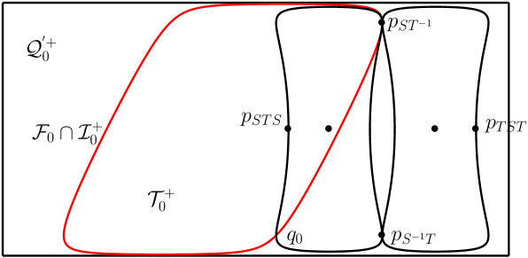
Figure 12: The intersection of $F_{0}$ with $\mathcal{I}_{0}^{+}$ drawn on $\mathcal{I}_{0}^{+}$, in geographical coordinates.

Let $D^{c}$ denote closure of the complement of $D$ in $\partial\mathbf{H}^{2}_{\mathbb{C}}-\{q_{\infty}\}$.

Proposition 7.12.

The closure of the intersection $D^{c}\cap D_{A}$ is a solid tube homeomorphic to a 3-ball.

Proof.

We describe the combinatorial cell structure of $D^{c}\cap D_{A}$; see Figure 14. Using Proposition 7.11, it is clear $D^{c}$ intersects $F_{0}$ in a topological disc whose boundary circle is made up of two edges, $c_{0}^{\pm}$ and two vertices $p_{ST^{-1}}$ and $q_{0}$. Combinatorially, this is a bigon. Applying $A^{-1}$ we see $D^{c}$ intersects $F_{-1}$ in a bigon with boundary made up of edges $c_{-1}^{\pm}$ and two vertices $p_{TST}$ and $q_{-1}$.

Moreover, Proposition 7.11 immediately implies that $c_{0}$ cuts $\mathcal{Q}_{0}^{\pm}$ into a quadrilateral and a triangle, which we denote by $\mathcal{{Q^{\prime}}}_{0}^{\pm}$ and $\mathcal{T}_{0}^{\pm}$. Since $D_{A}$ contains $p_{S^{-1}T}$ and $p_{TST}$, we see that $D_{A}$ contains $\mathcal{{Q^{\prime}}}_{0}^{+}$ and $\mathcal{T}_{0}^{-}$. These have vertex sets $\{p_{ST^{-1}},\,p_{TST},\,p_{S^{-1}T},\,q_{0}\}$ and $\{p_{S^{-1}T},\,p_{ST^{-1}},\,q_{0}\}$ respectively. Applying $A^{-1}$ we see that $c_{-1}$ cuts $\mathcal{Q}_{-1}^{\pm}$ into a quadrilateral, denoted $\mathcal{{Q^{\prime}}}_{-1}^{\pm}$, and a triangle, denoted $\mathcal{T}_{-1}^{\pm}$. Of these the quadrilateral $\mathcal{{Q^{\prime}}}_{-1}^{-}$ and the triangle $\mathcal{T}_{-1}^{+}$ lie in $D_{A}$. Finally, the bigons $\mathcal{B}_{0}^{+}$ and $\mathcal{B}_{-1}^{-}$ also lie in $D_{A}$.

In summary, the boundary of $D^{c}\cap D_{A}$ has a combinatorial cell structure with five vertices $\{p_{ST^{-1}},\,p_{S^{-1}T},\,p_{TST},\,q_{0},\,q_{-1}\}$ and eight faces.

$$\{\mathcal{Q^{\prime}}_{0}^{+},\,\mathcal{Q^{\prime}}_{-1}^{-},\,\mathcal{T}_{0}^{-},\,\mathcal{T}_{-1}^{+},\,\mathcal{B}_{0}^{+},\,\mathcal{B}_{-1}^{-},\,F_{0}\cap D^{c},\,F_{-1}\cap D^{c}\}.$$

These are respectively two quadrilaterals, two triangles and four bigons. Therefore, in total the cell structure has $(2\times 4+2\times 3+4\times 2)/2=11$ edges. Therefore the Euler characteristic of $\partial(D^{c}\cap D_{A})$ is

$$\chi\bigl{(}\partial(D^{c}\cap D_{A})\bigr{)}=5-11+8=2.$$

Hence $\partial(D^{c}\cap D_{A})$ is indeed a sphere. This means $D^{c}\cap D_{A}$ is a ball as claimed. ∎

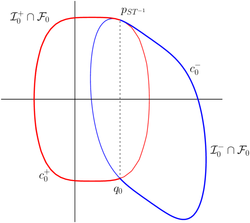
Figure 13: The intersection of $F_{0}$ with $\mathcal{I}_{0}^{+}\cap\mathcal{I}_{0}^{-}$. The disc $\mathcal{D}_{0}$ is the interior of $c_{0}=c_{0}^{+}\cap c_{0}^{-}$. The two segments $c_{0}^{+}$ and $c_{0}^{-}$ are the thicker parts of $F_{0}\cap\mathcal{I}_{0}^{+}$ and $F_{0}\cap\mathcal{I}_{0}^{-}$.

Figure 14: A combinatorial picture of the intersection of $\partial D$ with $D_{A}$ . The top and bottom lines are identified. The curve $c_{0}$ corresponds to the right hand side of the figure.

Remark 2.

The combinatorial structure described on Figure 14 is quite simple. However, the geometric realisation of this structure is much more intricate. As an example, there are fans $F$ parallel to $F_{0}$ and $F_{-1}$ whose intersection with $D^{c}$ is disconnected. This means that the foliation described right after Proposition 6.8 that is used in the proof of Theorem 6.4 is actually quite “distorted”.

We are now ready to prove Proposition 6.8.

Proposition 7.13.

There is a homeomorphism $\Psi_{A}:\mathbb{R}^{2}\times[0,1]\longrightarrow D_{A}$ that satisfies $\Psi_{A}(x,y,1)=A\Psi_{A}(x,y,0)$ and so that $\Psi_{A}$ restricts to a homeomorphism from the exterior of $S^{1}\times[0,1]$, that is $\bigl{\{}(x,y,z)\ :\ x^{2}+y^{2}\geq 1,\,0\leq z\leq 1\bigr{\}}$, to $D\cap D_{A}$.

Proof.

We have shown Proposition 7.12 that $D^{c}\cap D_{A}$ is a solid tube homeomorphic to a $3$-ball and (using Proposition 7.11) that $D^{c}$ intersects $\partial D_{A}$ in two discs, one in $F_{0}$ bounded by $c_{0}$ and the other in $F_{-1}$ bounded by $c_{-1}$. This means we can construct a homeomorphism $\Psi_{A}^{c}$ from the solid cylinder $\bigl{\{}(x,y,z)\ :\ x^{2}+y^{2}\leq 1,\,0\leq z\leq 1\bigr{\}}$ to $D^{c}\cap D_{A}$ so that the restriction of $\Psi_{A}^{c}$ to $S^{1}\times[0,1]$ is a homeomorphism to $\partial D\cap D_{A}$, with $\Psi_{A}^{c}:S^{1}\times\{0\}\longmapsto c_{-1}$ and $\Psi_{A}^{c}:S^{1}\times\{1\}\longmapsto c_{0}$. Adjusting $\Psi_{A}^{c}$ if necessary, we can assume that $\Psi_{A}^{c}(x,y,1)=A\Psi_{A}^{c}(x,y,0)$.

Furthermore, in Lemma 6.7, we showed that $D^{c}$ contains the invariant line $\Delta_{\varphi}$ of $\varphi$. This means that the cylinder $D^{c}\cap D_{A}$ is a thickening of $\Delta_{\varphi}\cap D_{A}$ and so, in particular, it cannot be knotted. Hence we can extend $\Psi_{A}^{c}$ to homeomorphism $\Psi_{A}:\mathbb{R}^{2}\times[0,1]\longrightarrow D_{A}$ satisfying $\Psi_{A}(x,y,1)=A\Psi_{A}(x,y,0)$. In particular, $\Psi$ maps $\bigl{\{}(x,y,z)\ :\ x^{2}+y^{2}\geq 1,\,0\leq z\leq 1\bigr{\}}$ homeomorphically to $D\cap D_{A}$ as claimed. ∎

Finally, we prove Proposition 6.8 by extending $\Psi_{A}:\mathbb{R}^{2}\times[0,1]\longrightarrow D_{A}$ equivariantly to a homeomorphism $\Psi:\mathbb{R}^{3}\longmapsto\partial\mathbf{H}^{2}_{\mathbb{C}}-\{q_{\infty}\}$. That is, if $(x,y,z+k)\in\mathbb{R}^{3}$ where $k\in{\mathbb{Z}}$ and $z\in[0,1]$, we define $\Psi(x,y,z+k)=A^{k}(x,y,z)$. Since $\Psi(x,y,1)=A\Psi(x,y,0)$ there is no ambiguity at the boundary.

References

- [1] H. Akiyoshi, M. Sakuma, M. Wada, and Y. Yamashita. Punctured Torus Groups and 2-Bridge Knot Groups I. Springer LNM 1909, Heidelberg, 2007.
- [2] A.F. Beardon. The geometry of discrete groups. Springer, New York, 1983.
- [3] S. Chen and L. Greenberg. Hyperbolic spaces. In Contribution to Analysis, pages 49–87. Academic Press, New York, 1974.
- [4] D. Cooper, D. Long, and M. Thistlethwaite. Flexing closed hyperbolic manifolds. Geom. Topo., 11:2413–2440, 2007.
- [5] M. Culler, N. M. Dunfield, and J. R. Weeks. SnapPy, a computer program for studying the topology of -manifolds. Available at http://snappy.computop.org.
- [6] M. Deraux. A 1-parameter family of spherical CR uniformisations of the fighure eight knot complement. arxiv:1410.1198.
- [7] M. Deraux. On spherical CR uniformization of 3-manifolds. Exp. Math., 24:355–370, 2015.
- [8] M. Deraux and E. Falbel. Complex hyperbolic geometry of the figure eight knot. Geom. Topol., 19:237–293, 2015.
- [9] M. Deraux, J.R. Parker, and J. Paupert. New non-arithmetic complex hyperbolic lattices. Invent. Math., 203:681–771, 2016.
- [10] D. B. Epstein and C. Petronio. An exposition of oincaré’s polyhedron theorem. Enseign. Math. (2), 40(1-2):113–170, 1994.
- [11] E. Falbel. A spherical CR structure on the complement of the figure eight knot with discrete holonomy. Journal Diff. Geom., 79(1):69–110, 2008.
- [12] E. Falbel, A. Guilloux, P.V. Koseleff, F. Rouillier, and M. Thistlethwaite. Character varieties for SL(3, : the figure eight knot. arXiv:1412.4711, 2014.
- [13] E. Falbel, P.V. Koseleff, and F. Rouillier. Representations of fundamental groups of 3-manifolds into : exact computations in low complexity. Geometriae Dedicata, 177:229–255, 2015.
- [14] E. Falbel and J.R. Parker. The geometry of the Eisenstein-Picard modular group. Duke Math. J., 131(2):249–289, 2006.
- [15] W.M. Goldman. Complex Hyperbolic Geometry. Oxford University Press, Oxford, 1999.
- [16] W.M. Goldman and J.R. Parker. Complex hyperbolic ideal triangle groups. Journal für dir reine und angewandte Math., 425:71–86, 1992.
- [17] W.M. Goldman and J.R. Parker. Dirichlet Polyhedra for Dihedral Groups Acting on Complex Hyperbolic Space. Jour. Geom. Analysis, 2(6):517–554, 1992.
- [18] M. Heusener, V. Munoz, and J. Porti. The SL(3,)-character variety of the figure eight knot. arXiv:1505.04451, 2015.
- [19] L. Keen and C. Series. The Riley slice of Shottky space. Proc. London Math. Soc, 69:72–90, 1994.
- [20] B. Martelli and C. Petronio. Dehn filling of the ’magic’ 3-manifold. Comm. Anal. Geom., 14:967–1024, 2006.
- [21] G. Martin. On discrete isometry groups of negative curvature. Pacific J. Math., 160:109–128, 1993.
- [22] G.D. Mostow. A remarkable class of polyhedra in complex hyperbolic space. Pac. J. Math., 86:171–276, 1980.
- [23] J. Parker and P. Will. Complex hyperbolic free groups with many parabolic elements. In Geometry, Groups and Dynamics, volume 639 of Contemporary Mathematics, pages 327–348. American Mathematical Society, Providence, RI, 2015.
- [24] J.R. Parker. Complex Hyperbolic Kleinian Groups. Cambridge University Press, to appear,.
- [25] J.R. Parker and I.D. Platis. Complex hyperbolic quasi-Fuchsian groups. In Geometry of Riemann Surfaces, volume 368 of London Mathematical Society Lecture Notes, pages 309–355. 2010.
- [26] J.R. Parker, Jieyan Wang, and Baohua Xie. Complex hyperbolic triangle groups. Pacific. J. Mathematics, 280:433–453, 2016.
- [27] J. Paupert and P. Will. Real reflections, commutators and cross-ratios in complex hyperbolic space. Preprint arXiv:1312.3173.
- [28] A. Pratoussevitch. Traces in complex hyperbolic triangle groups. Geometriae Dedicata, 111:159–185, 2005.
- [29] J.G. Ratcliffe. Foundations of Hyperbolic Manifolds. Springer-Verlag, New York, 2006.
- [30] R. E. Schwartz. Degenerating the complex hyperbolic ideal triangle groups. Acta Math., 186:105–154, 2001.
- [31] R. E. Schwartz. Ideal triangle groups, dented tori, and numerical analysis. Ann. of Math. (2), 153:533–598, 2001.
- [32] R. E. Schwartz. Complex hyperbolic triangle groups. Proc. Int. Math. Cong., 1:339–350, 2002.
- [33] R. E. Schwartz. A better proof of the Goldman-Parker conjecture. Geometry and Topology, 9:1539–1601, 2005.
- [34] R. E. Schwartz. Spherical CR Geometry and Dehn Surgery, volume 165 of Ann. of Math. Studies. Princeton University Press, Princeton, 2007.
- [35] W. Thurston. The Geometry and Topology of Three-Manifolds. http://www.msri.org/publications/books/gt3m/.
- [36] P. Will. Traces, Cross-ratios and 2-Generator Subgroups of PU(2,1). Canad. J. Math., 61(6):189–209, 2009.
- [37] P. Will. Bending Fuchsian representations of fundamental groups of cusped surfaces PU(2,1). Jour. Differ. Geom., 90(3):473–520, 2012.
- [38] P. Will. Two-generator groups acting on the complex hyperbolic plane. In Handbook of Teichmüller theory. Vol. VI, IRMA Lect. Math. Theor. Phys. Eur. Math. Soc., Zürich, to appear.