An extension of the open-source porousMultiphaseFoam toolbox dedicated to groundwater flows solving the Richards’ equation

Abstract

In this note, the existing porousMultiphaseFoam toolbox, developed initially for any two-phase flow in porous media is extended to the specific case of the Richards’ equation which neglect the pressure gradient of the non-wetting phase. This model is typically used for saturated and unsaturated groundwater flows. A Picard’s algorithm is implemented to linearize and solve the Richards’ equation developed in the pressure head based form. This new solver of the porousMultiphaseFoam toolbox is named groundwaterFoam. The validation of thesolver is achieved by a comparison between numerical simulations and results obtained from the literature. Finally, a parallel efficiency test is performed on a large unstructured mesh and exhibits a super-linear behavior as observed for the other solvers of the toolbox.

1 Introduction

The modeling and understanding of fluid flow in unsaturated soils is an important problem in a wide range of scientific domains, such as environmental engineering or groundwater hydrology. Two-phase flow in porous media can be modeled by solving the mass conservation equation for each phase where the phase velocities are expressed using a generalized Darcy’s law [10]. However, a classical approach commonly used in soils science consists in neglecting the pressure gradient in the non-wetting phase (typically the air) to reduce the two-phase flow to one equation, the so-called Richards’ equation [13, 5].

Several softwares has been developed to solve the Richards’ equation and some of these developments have already been done using the OpenFOAM platform [7, 14]. We can cite the example of Liu [9] who developed a saturated-unsaturated groundwater flow solver based on the Picard’s algorithm. This solver includes several features such as the different forms of the Richards equation (pressure-based and mixed-form), three convergence criteria and specific boundary conditions. More recently, another Richards’ solver has also been proposed for the OpenFOAM platform [11]. Both initiatives have been shown to have good parallel efficiency.

In a previous work, an open-source toolbox based on OpenFOAM and dedicated to the simulation of multiphase flow in porous media as been developed and validated [6]. Based on the IMPES method (Implicit Pressure Explicit Saturation) [15], this toolbox includes the commonly used porous media models (relative permeability, capillary pressure), specific boundary conditions and validation cases. A good parallel efficiency has also been demonstrated. This project is still under development and the toolbox is freely available [2].

To expand the possibilities and the application fields of the porous media toolbox, this work proposes to implement a version of the Richards’ equation following the formalism of the toolbox and re-using as much as possible the existing libraries. First, the mathematical model and the formulation chosen are presented. In Sec. 3, the numerical implementation is developed with the different choices in terms of time step determination, algorithm, etc. The solver is then validated and evaluated in terms of parallel efficiency in Sec. 4. In the following, italic style refers to solvers, small capitals style to libraries, and typewriter style to directories.

2 Mathematical model

Three major forms of the unsaturated mass conservation equation exist in the literature: the pressure head-based, the saturation-based or the mixed-form formulation. The pressure head-based formulation has been chosen as this formulation is closed to the previously developed solvers of the toolbox [6]. The Richards’ equation in the pressure head based formulation reads

$$C(h)\frac{\partial h}{\partial t}-\nabla\cdot\left[K_{S}(h)\nabla\left(h+z\right)\right]=0,$$ (1)

where $h$ is the pressure head, $C(h)$ the capillary capacity depending on the head pressure, $K_{S}(h)$ the hydraulic conductivity and $z$ the elevation. This equation can be formulated as

$$C(h)\frac{\partial h}{\partial t}-\nabla\cdot\left[M_{\theta}\left(\rho_{\theta}\parallel\mathbf{g}\parallel_{2}\nabla h-\rho_{\theta}\mathbf{g}\right)\right]=0,$$ (2)

where $\rho_{\theta}$ is the phase density, $\parallel\mathbf{g}\parallel_{2}$ the magnitude of the gravity field and $M_{\theta}$ the phase mobility of the phase defined as

$$M_{\theta}=\frac{Kk_{r,\theta}}{\mu_{\theta}},$$ (3)

where $K$ is the intrinsic permeability of the porous medium, $\mu_{\theta}$ the liquid viscosity and $k_{r,\theta}$ the relative permeability. The saturated hydraulic conductivity $K_{S}$, commonly used for fluid flow in unsaturated soils, is then directly related to the rock intrinsic permeability following:

$$K=\frac{\mu_{\theta}K_{S}}{\rho_{\theta}\parallel\mathbf{g}\parallel_{2}}.$$ (4)

Note that the relative permeability $k_{r,\theta}$ is expressed as a function of saturation $\theta$ to re-use the already implemented relative permeability models (Brooks and Corey [3], Van Genuchten [16]). Using this formulation, only two functions need to be added in the capillaryModel library. The first one allows to compute the saturation $\theta$ from the pressure head $h$, which gives, for the Van Genuchten model,

$$\theta(h)=\left\{\begin{array}[]{ll}\frac{\theta_{s}-\theta_{r}}{\left((1+(\alpha|h|))^{n}\right)^{m}}+\theta_{r}&\forall\,h<0\\ \theta_{s}&\forall\,h\geq 0\end{array}\right.$$ (5)

where $\theta_{s}$ and $\theta_{r}$ are respectively the saturated and residual saturations, and $\alpha$ and $m$ the Van Genuchten’s parameters. The second function computes the capillary capacity

$$C(h)=\frac{\alpha m\left(\theta_{s}-\theta_{r}\right)}{1-m}\left(\theta_{e}\right)^{\frac{1}{m}}\left(1-\left(\theta_{e}\right)^{\frac{1}{m}}\right)^{m}$$ (6)

where $\theta_{e}$ is the effective saturation given by

$$\theta_{e}=\frac{\theta(h)-\theta_{r}}{\theta_{s}-\theta_{r}}.$$

The total mobility $M$ is defined as

$$M=M_{\theta}\rho_{\theta}\parallel\mathbf{g}\parallel_{2}$$ (7)

which allows to directly use the existing darcyGradPressure boundary condition for the pressure head field $h$. When using this boundary conditions, the solver will look up at the fixed value for the velocity field $U$, and the value of total mobility $M$ to set the pressure head gradient necessary to impose the fluid velocity. Readers can refer to the work of Horgue et al. [6] for more details about the darcyGradPressure boundary condition.

3 Numerical implementation

Different iterative techniques can be used to solve the non-linear problem expressed in Eq. (2) including Picard and Newton methods. The Picard method has been implemented in this work as it the simplest and the more robust technique. Note that a better convergence rate can be obtained with Newton methods but this requires the computation of a Jacobian matrix (increasing the RAM memory required).

3.1 Picard’s algorithm

In the Picard method, the pressure-head field $h^{n+1,m+1}$ for the iteration $m+1$ of the algorithm is computed as:

$$C(h^{n+1,m})\frac{h^{n+1,m+1}-h^{n}}{\Delta t^{n}}-\nabla\cdot\left(\rho_{\theta}\parallel\mathbf{g}\parallel_{2}M_{\theta}^{n+1,m}\nabla h^{n+1,m+1}\right)+\nabla M_{\theta}^{n+1,m}\cdot\rho_{\theta}\mathbf{g}=0$$ (8)

with $h^{n}$ the head pressure value at the last time $n$ and $M^{n+1,m}$the phase mobility computed using the last iteration $h^{n+1,m}$. The loop occurs until the Picard residual $r_{Picard}$ satisfies:

$$r_{Picard}=max\left(\mid h^{n+1,m+1}-h^{n+1,m}\mid\right)<\epsilon{}_{Picard}$$ (9)

where $\epsilon{}_{Picard}$ is the user-defined Picard tolerance.

3.2 Time-step

A simple heuristic way has been chosen as proposed in [17] for time step determination with a stabilization parameter to avoid too sharp time-step evolution. This includes three user-defined numbers of iterations ($n_{maxIter,Picard}$, $n_{minIter,Picard}$ and $n_{maxIter,stabilization}$) and two time-step factors ($f_{\Delta t,increase}$ and $f_{\Delta t,decrease}$). After the Picard algorithm has converged using $n_{iter,Picard}$ iterations, three different situations can occur:

1. $n_{iter,Picard}>n_{maxIter,Picard}$, the current time step is too large and $\Delta t^{n+1}=f_{\Delta t,decrease}\times\Delta t^{n}$.

2. $n_{minIter,Picard}\leq n_{iter,Picard}\leq n_{maxIter,Picard}$, the time step remains unchanged $\Delta t^{n+1}=\Delta t^{n}$.

3. $n_{iter,Picard}<n_{minIter,Picard}$:

   1. the stabilized iteration counter is increased: $n_{iter,stabilized}=n_{iter,stabilized}+1$

   2. If $n_{iter,stabilized}=n_{maxIter,stabilization}$, then the time step increases $\Delta t^{n+1}=f_{\Delta t,increase}\times\Delta t^{n}$ and the counter is reseted ($n_{iter,stabilized}=0$).

3.3 Algorithm

The global algorithm for each time step consists in:

1. While $r_{Picard}>\epsilon{}_{Picard}$

   1. solve Richards’ equation (8)

   2. update flow properties (relative permeabilities, capillary pressure)

   3. compute Picard residual $r_{Picard}$

   4. if $n_{iter,Picard}>2\times n_{maxIter,Picard}$: break loop, accept current solution and display warning message

2. Compute $\Delta t$ for the next iteration (see Sec. 3.2).

3.4 Code structure

The program groundwaterFoam, solving the Richards’ equation for an heterogeneous isotropic permeability field ($K$ is an heterogeneous scalar field) have been added to the porousMultiphaseFoam toolbox. Note that, following the example of impesFoam and anisoImpesFoam, it is possible to develop a Richards’ solver handling anisotropic permeability fields. The capillarityModels functions have been modified to compute saturation $\theta$ and capillary capacity $C(h)$ from head pressure $h$. Note that the Van Genuchten model is currently the only model implemented in the toolbox.

Three test cases have been added in the groundwaterFoam-tutorials folder of the toolbox. The 1Dinfiltration simulation is used to validate the developed solver (see Sec. 4.1) and provides an example of the solver use. The 1Dinfiltration_Ufixed is close to the previous validation case but using the darcyGradPressure boundary condition (which set the value of the velocity field). The realCase provides an example on a more complex geometry based on real topographic dataset and has been used to evaluate parallel efficiency (see Sec. 4.2).

4 Numerical simulations

4.1 Validation case

The vertical 1D water infiltration problem proposed for validation is derived from the work of Celia et al. [4] and has been used in several studies [12, 8]. The column of New Mexico soils is modeled using the following parameter:

• $K_{s}=0.00922$ cm.s^-1 (corresponding to $K=9.4.10^{-12}$ m²),

• $\theta_{r}=0.102$ and $\theta_{s}=0.368$,

• $\alpha=0.0335$ cm^-1,

• $m=1-\frac{1}{n}=0.5$,

• $\mu_{\theta}=1\cdot 10^{-3}$ Pa.s,

• $\rho_{\theta}=1\cdot 10^{3}$ kg.m^-3.

The boundary condition on the top of the column is initialized to $h=-75$ cm (corresponding to $\theta=0.20037$) while the head pressure is uniformly distributed in the column $h=-1000$ cm (corresponding to $\theta=0.10994$). The domain is discretized using $200$ computation cells and the test case is directly available in the toolbox tutorials (1Dinfiltration folder).

The comparison between simulations and the reference solution (numerical results extracted from the work of Kavetski et al. [8]) presented in Fig. 1 shows a good agreement and validates the code.

Figure 1: Pressure head profiles at various times for the 1D infiltration case (lines are reference results from Kavetski et al. [8])

4.2 Parallel efficiency

The test of the parallel efficiency is performed on a 3D unstructured mesh constructed on real topographic dataset. For this purpose, the software MMesh3D developed by S. Marras is used [1] which allows to build standard mesh files in the VTK format. Using the topographic dataset of the Monterey bay in California (dataset available with the software), a coarse unstructured mesh composed by $60\times 120\times 10$ ($72\,000$) computation cells is constructed in the VTK format and then transformed into the OpenFOAM format using the utility vtkUnstructuredToFoam. Figure 2 shows the mesh with an aspect ratio of $1:1:4$. The permeability field, randomly distributed with a uniform law ($K\in\left[9.4.10^{-13}:9.4.10^{-12}\right]$ m²), is shown in Fig. 3. The pressure head is initialized in the full domain with an homogeneous value $h_{init}=-5$ m ($\theta_{init}\approx 0.118$) and a fixed pressure head $h_{top}=-0.5$ m ($\theta_{top}\approx 0.306$) is imposed on the top of the domain (the irregular face). The other parameters used for this test are identical to those used in the Sec. 4.1. An example of the saturation field at $t=1000$ days using the coarse mesh is presented in Figure 4.

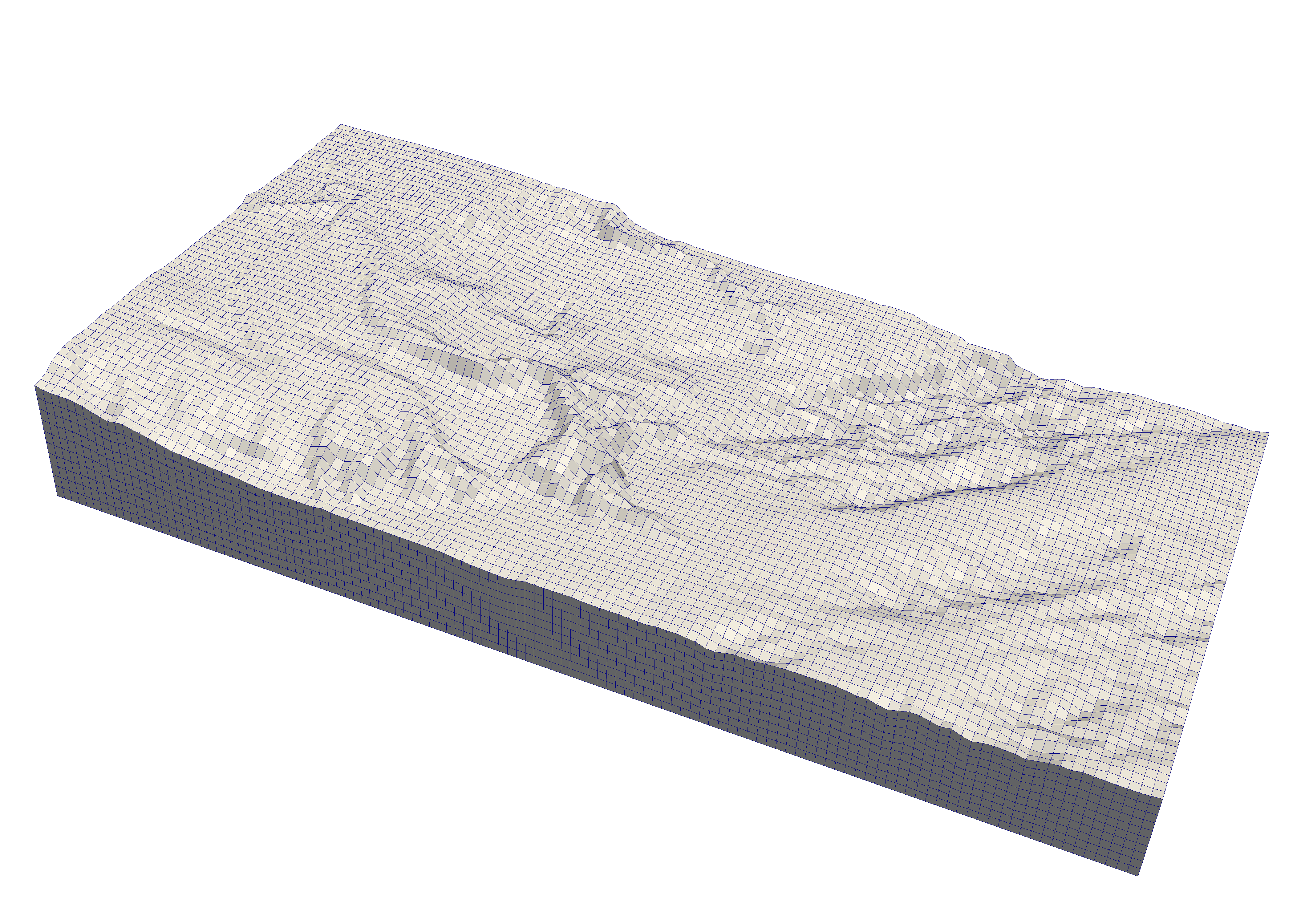
Figure 2: Unstructured coarse mesh based on real topographic dataset (aspect ratio of the visualization $1:1:4$)

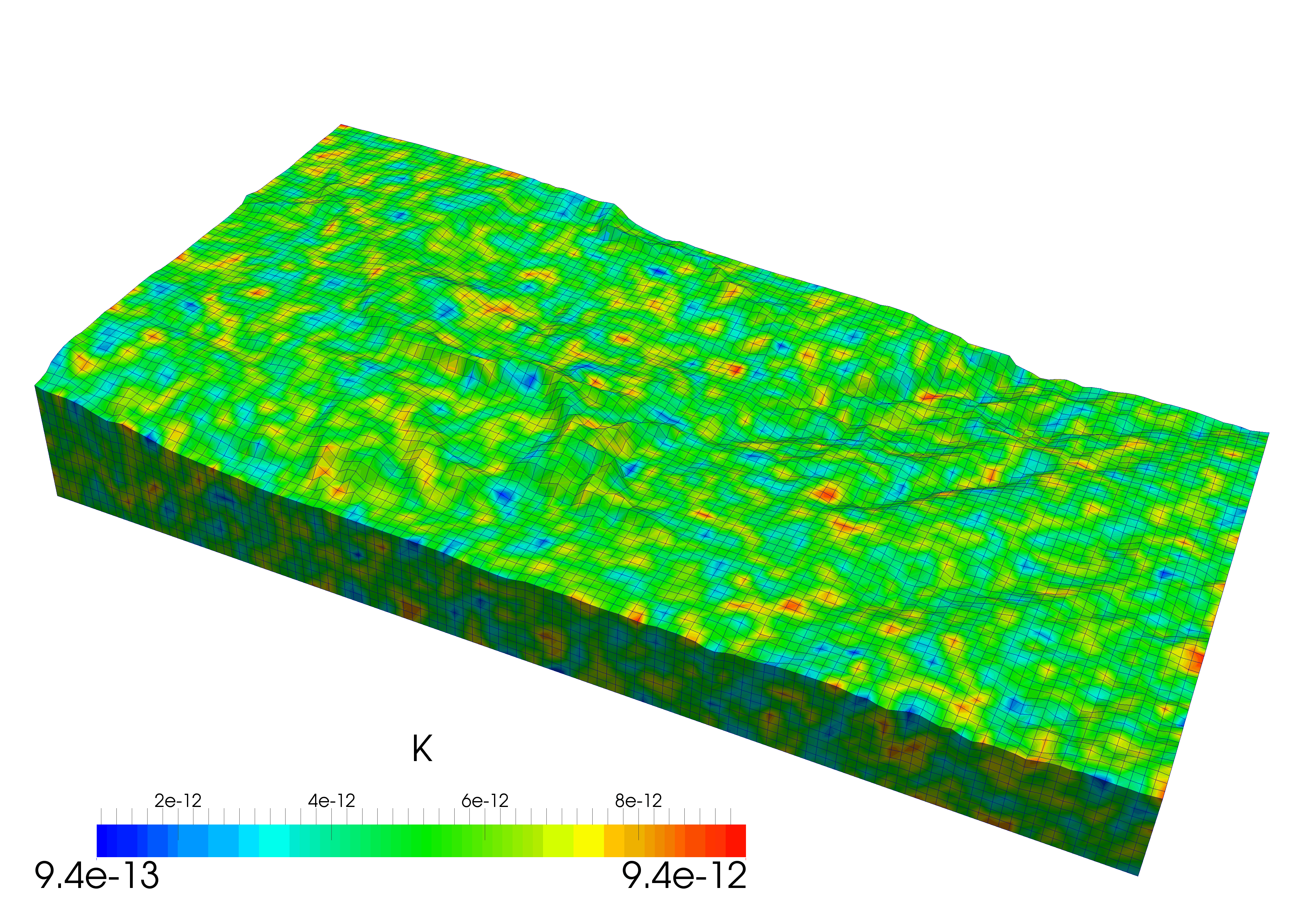
Figure 3: Uniformly distributed permeability field

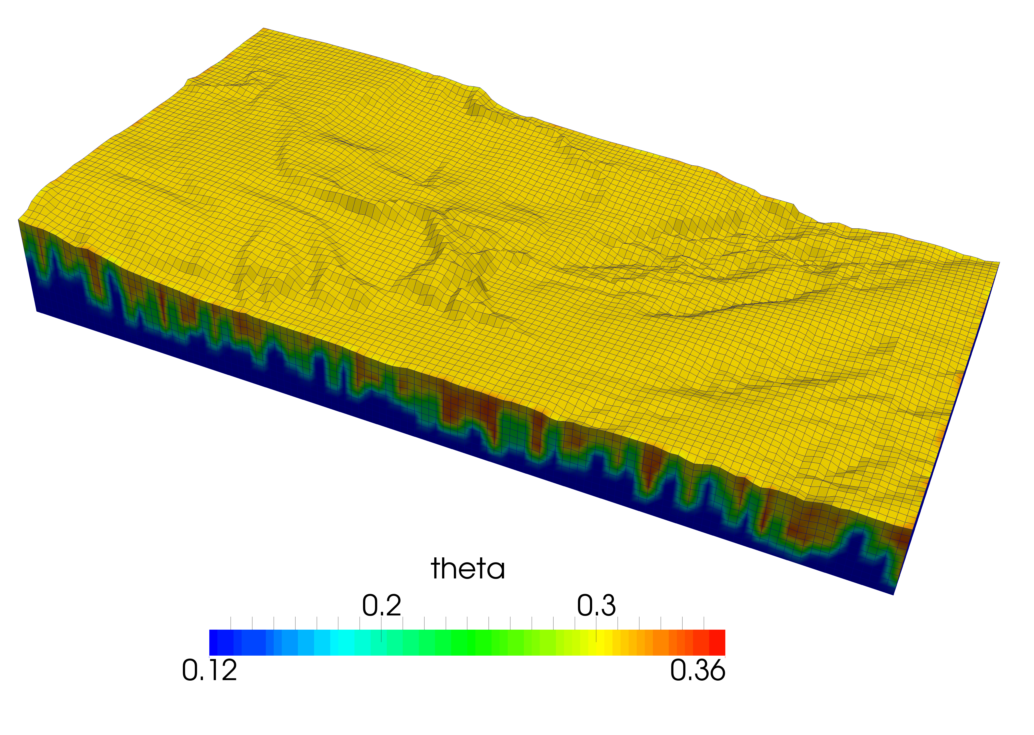
Figure 4: Saturation field at $t=1000$ days

To increase the size of the problem (necessary for the strong scaling evaluation), the utility refineMesh is used twice to multiply by $64$ the mesh size ($240\times 480\times 40=4\,608\,000$ computation cells). The infiltration phenomenon is then simulated on the CALMIP’s EOS cluster which consists of $612$ computation nodes of 2 Intel processors 10-cores clocked at $2.8$ GHz. Simulations are performed from $20$ (the reference) to $1280$ cores (corresponding to $64$ computation nodes) and the total CPU time required for the full simulation is about $12$ hours. The maximum amount of memory used by the process is $\sim 5500$ Mb. The speedup $\sigma$ for a simulation with $n$ cores is computed as

$$\sigma_{n}=\frac{T_{20}}{T_{n}}$$ (10)

where $T_{n}$ is the computation time for $n$ cores. The speedup of the groundwaterFoam solver is shown in Figure 5 and exhibits a super-linear speedup until $640$ cores. This behavior has previously been observed with the previous developed solver of the toolbox [6]. We should note that the parallel efficiency is almost linear for $1280$ cores and probably decreases for a larger number of processors. This may be explained by the fact that the linear system for each computation core becomes too small ($3600$ mesh cells per core for $1280$ cores). In this configuration, the parallel efficiency allows to reduce the computation time from $\sim 34$ min ($20$ cores) to $\sim 36$ seconds ($1280$ cores).

Figure 5: Log-log representation of the speedup with the $groundwaterFoam$ solver (reference is one computation node of $20$ cores)

5 Conclusion

In this work, an OpenFOAM® solver dedicated to the Richards’ equation has been developed to extend the scope of the porousMultiphaseFoam toolbox [2]. The specific form of Van Genuchten’s model has been implemented to allow groundwater flow simulations with the groundwaterFoam solver. Three test cases are provided with the freely accessible toolbox:

1. The 1D infiltration case which validates the numerical implementation of the model by a comparison with results from the literature.

2. A 1D infiltration case with inlet velocity fixed which shows an example of using the boundary condition darcyGradPressure.

3. A real topographic case with an unstructured mesh that has been used to evaluate the parallel efficiency of the solver and exhibits a super-linear behavior.

References

References

- [1] MMesh3D. URL http://mmesh3d.wikispaces.com/.
- Hor [2015] The porousmultiphasefoam toolbox, 2015. URL https://github.com/phorgue/porousMultiphaseFoam.git.
- Brooks and Corey [1964] R. H. Brooks and A. T. Corey. Hydraulic Properties of Porous Media. In Hydrology Papers, 1964.
- Celia et al. [1990] M. A. Celia, E. T. Bouloutas, and R. L. Zarba. A general mass-conservative numerical solution for the unsaturated flow equation. Water Resources Research, 26, 1990.
- Hillel [1980] D. Hillel. Fundamentals of soil physics. 1980.
- Horgue et al. [2015] P. Horgue, C. Soulaine, J. Franc, R. Guibert, and G. Debenest. An open-source toolbox for multiphase flow in porous media. Computer Physics Communications, 187, 2015.
- Jasak [1996] H. Jasak. Error Analysis and Estimation for the Finite Volume Method with Applications to Fluid Flows, 1996.
- Kavetski et al. [2001] D. Kavetski, P. Binning, and S. W. Sloan. Adaptive time stepping and error control in a mass conservative numerical solution of the mixed form of Richards equation. Advances in Water Resources, 24, 2001.
- Liu [2012] X. Liu. suGWFoam: An Open Source Saturated-Unsaturated GroundWater Flow Solver based on OpenFOAM, Civil and Environmental Engineering Studies Technical Report No. 01-01. Technical report, 2012.
- Muskat [1949] M. Muskat. Physical principles of oil production. New York, mcgraw-hil edition, 1949.
- Orgogozo et al. [2014] L. Orgogozo, N. Renon, C. Soulaine, F. Hénon, S. K. Tomer, D. Labat, O. S. Pokrovsky, M. Sekhar, R. Ababou, and M. Quintard. An open source massively parallel solver for Richards equation: Mechanistic modelling of water fluxes at the watershed scale. Computer Physics Communications, 185, 2014.
- Rathfelder and Abriola [1994] K. Rathfelder and L. M. Abriola. Mass conservative numerical solutions of the head-based Richards equation. Water Resources Research, 1994.
- Richards [1931] L. A. Richards. Capillary conduction of liquids through porous mediums. Journal of Applied Physics, 1931.
- Rusche [2002] H. Rusche. Computational fluid dynamics of dispersed two-phase flows at high phase fractions. PhD thesis, 2002.
- Sheldon et al. [1959] J. W. Sheldon, B. Zondek, and W. T. Cardwell. One-dimensional, incompressible, non-capillary, two-phase fluid flow in a porous medium. T. SPE. AIME, 1959.
- Van Genuchten [1980] M. T. Van Genuchten. A Closed-form Equation for Predicting the Hydraulic Conductivity of Unsaturated Soils1. Soil Science Society of America Journal, 44, 1980.
- Williams and Miller [1999] G. A. Williams and C. T. Miller. An evaluation of temporally adaptive transformation approaches for solving richards’ equation. Advances in Water Resources, 1999.