On the upper limits for dipole anisotropies in cosmic-ray positrons

Abstract

The excess of cosmic-ray positrons in the energy range from 10 GeV to few hundred GeV reported by PAMELA and AMS experiments is not consistent with a pure secondary origin and requires the introduction of a source term. The presence of anisotropies in the positron arrival directions would be a distinctive signature of their origin. Current measurements are consistent with isotropy and limits to a dipole anisotropy have been established. In this note, we review the mathematical basis of this analysis and provide a general bound to the dipole upper limits achievable from a given sample of events. The published experimental limits are confronted with this bound.

1 Introduction

Recent measurements of the cosmic-ray positrons carried out by the PAMELA [1] and AMS [2] space spectrometers have provided precise characterization of their energy spectrum up to few hundred GeV. In particular, the positron spectrum above $\sim$20 GeV is harder than the electron spectrum and therefore, the positron fraction shows a striking increase dubbed as positron excess [3, 4].

The pure secondary production of positrons, originated from the interaction of primary cosmic rays with the interstellar medium, can not account for the features in the observed spectrum. Additional source terms for positron and electrons are needed to reproduce the measurements.

The physical origin of the source term has been extensively discussed. The proposed models can be grouped into three different classes. First, secondary production in the standard cosmic ray sources [5]; second, exotic astrophysical sources, e.g. pulsars [6]; finally, dark matter annihilation in the galactic halo [7] or in the Earth’s vicinity [8]. The detection of anisotropies in the positron arrival directions would certainly favor some of these hypotheses.

Searches for large scale anisotropies in the positron samples have been carried out by the experiments [10, 11]. The result is that the distribution of the arrival directions is consistent with isotropy and thus, limits may be set to the anisotropies at different angular scales. In particular, an upper limit to a dipole anisotropy can be established within a certain confidence level.

In this note we present a short review of the mathematical rationale behind the analysis of dipole anisotropies and the confidence regions one may achieve from an experiment. The basic definitions are introduced in section 2. In section 3, the expressions for the lower bound to the one-side confidence regions to a dipole anisotropy and the expected limit from a single experiment are obtained. In section 4, we discuss the consistency with the published limits by the AMS and PAMELA collaborations.

2 Basic Formulae

The angular distribution of cosmic rays is described by a probability density function $p({\theta},{\phi}|{\bullet}){\in}L_{2}({\Omega})$, which is a real, non-negative and well-behaved function with support in ${\Omega}=[0,{\pi}]{\times}[0,2{\pi}]$. The analysis of anisotropies is based on the expansion of this density in a spherical harmonics basis. Being a real function, it is natural to use the orthonormal real harmonics basis (therefore real coefficients), though irrelevant for what follows. Thus, after normalization, we can write

$$p({\theta},{\phi}|\mbox{{\boldmath${a}$}})\,=\,\frac{\textstyle 1}{\textstyle 4{\pi}}\,\left(1\,+\,a_{lm}\,Y_{lm}({\theta},{\phi})\right)$$ (1)

where $\mbox{{\boldmath${a}$}}=\{a_{lm};\,l{\geq}1,-l{\leq}m{\leq}l\}$,

$$a_{lm}\,=\,4{\pi}\int_{\Omega}p({\theta},{\phi})\,Y_{lm}({\theta},{\phi})\,d{\mu}\,=\,4{\pi}\,E_{p;{\mu}}[Y_{lm}({\theta},{\phi})]\,,$$ (2)

$d{\mu}=\sin{\theta}d{\theta}d{\phi}$ and summation over repeated indices is understood. In this note, we shall be particularly interested in dipole anisotropies $(l=1)$ so, to simplify the notation, we redefine the indices $(l,m)=\{(1,-1),(1,0),(1,1)\}$ as $i=\{1,2,3\}$ and write

$$p({\theta},{\phi}|\mbox{{\boldmath${a}$}})\,=\,\frac{1}{4{\pi}}\,\left(1\,+\,a_{1}Y_{1}\,+\,a_{2}Y_{2}\,+\,a_{3}Y_{3}\right)$$ (3)

with $\mbox{{\boldmath${a}$}}=(a_{1},a_{2},a_{3})$.

The coefficient of dipole anisotropy

$${\delta}\,=\,\sqrt{\frac{3}{4{\pi}}}\,\left(a_{1}^{2}\,+\,a_{2}^{2}\,+\,a_{3}^{2}\right)^{1/2}$$ (4)

corresponds to the usual definition  [3, 4] based on the maximum and minimum values of the intensity of Cosmic Rays.

Obviously, for any $({\theta},{\phi}){\in}{\Omega}$ we have that $p({\theta},{\phi}|\mbox{{\boldmath${a}$}}){\geq}0$ so the set of parameters ${a}$ are constrained on a compact support. In the present case, non-negativity of the probability density implies that the dipole coefficients are bounded by the sphere

$$a_{1}^{2}\,+\,a_{2}^{2}\,+\,a_{3}^{2}\,{\leq}\,\frac{4{\pi}}{3}$$ (5)

and therefore, the coefficient of dipole anisotropy by ${\delta}\,{\leq}\,1$.

3 Parametric Inference

Given an exchangeable sequence $\{x_{1},x_{1},{\ldots},x_{n}\}$ of $n$ observations $x_{i}=({\theta}_{i},{\phi}_{i})$ identically distributed from the parametric model $p({\theta},{\phi}|\mbox{{\boldmath${a}$}})$, we shall be interested in making inferences on the parameters $\mbox{{\boldmath${a}$}}=(a_{1},a_{2},a_{3})$ from the proper posterior density,

$$p(\mbox{{\boldmath${a}$}}|{\bullet})\,{\propto}\,\pi(\mbox{{\boldmath${a}$}})\,\prod_{i=1}^{n}\,p({\theta}_{i},{\phi}_{i}|\mbox{{\boldmath${a}$}})$$ (6)

with $\pi(\mbox{{\boldmath${a}$}})$ the reference prior and, eventually, on the dipole anisotropy coefficient $\delta$ from $p({\delta}|{\rm data})$.

3.1 Expected precision on the dipole coefficients

The first question to address is the precision we expect on the parameters ${a}$ given a sequence of observations. The space of parameters ${S}_{\mbox{{\boldmath${a}$}}}$ is a Riemannian manifold with the Fisher-Rao metric tensor given by:

$$g_{ij}(\mbox{{\boldmath${a}$}})\,=\,\frac{1}{(4{\pi})^{2}}\,\int_{\Omega}\,\frac{Y_{i}({\theta},{\phi})\,Y_{j}({\theta},{\phi})}{p({\theta},{\phi}|\mbox{{\boldmath${a}$}})}\,d{\mu}\,.$$ (7)

We shall be interested in a neighborhood of $\mbox{{\boldmath${a}$}}=(0,0,0)$ so, expanding this expression to order ${\sl O}({a}_{i}^{4})$ one gets:

$$g_{ij}\,{\simeq}\,\frac{1}{4{\pi}}(1\,+\,\frac{{\delta}^{2}}{5})\,{\delta}_{ij}\,+\,\frac{6}{5(4{\pi})^{2}}\,{a}_{i}{a}_{j}\,.$$ (8)

Regularity conditions are satisfied to ensure that, for large $n$, the posterior density $p(\mbox{{\boldmath${a}$}}|{\bullet})$ is asymptotically normal. Then, for large $n$, prior precision can be ignored compared to that from data and the accuracy will be given by the Hessian matrix. Thus, again to order ${\sl O}({a}_{i}^{4})$, we have that:

$$V({a}_{i},{a}_{i})\,\simeq\,\frac{4{\pi}}{n}\,\left(1\,-\,\frac{3}{5(4{\pi})}\left({a}_{1}^{2}\,+\,{a}_{2}^{2}\,+\,{a}_{3}^{2}\,+\,2\,{a}_{i}^{2}\right)\right)$$ (9)

and covariances

$$V({a}_{i},{a}_{j})\,\simeq\,-\frac{6}{5\,n}\,{a}_{i}{a}_{j}\hskip 42.67912pti{\neq}j.$$ (10)

In particular, in the limit ${a}_{1,2,3}{\rightarrow}0$ one has

$${\sigma}({a}_{i})\,=\,\sqrt{\frac{4{\pi}}{n}}\hskip 28.45274pt{\rm and}\hskip 28.45274pt{\rho}_{ij}\,=\,0\,.$$ (11)

A question that has been posed is whether one can have more precise estimates. First, one can obviously rotate the reference frame to increase the sensitivity in one particular direction. However, on the one hand, if the coefficients $a_{i}$ have small absolute value the changes in the Hessian matrix will be of order ${\sl O}({a}_{i}^{2})$. On the other hand, rotations are orthogonal transformations, isometric, so for a second order tensor $G$ there are three quantities that remain invariant (Cayley-Hamilton) and they ensure that, to order ${\sl O}({a}_{i}^{2})$, $\sum{\sigma}^{2}(a_{i})$ and $\prod{\sigma}^{2}(a_{i})$ will not change. In consequence, any improvement in the accuracy of one parameter has to be compensated by the worsening of the accuracy of the other parameters and therefore there is no way to improve the precision of the coefficient of dipole anisotropy in a significant manner by rotations of the reference frame.

In a more realistic situation, two effects have to be considered. First, it may happen that only a fraction of ${\Omega}$ is experimentally observed. This can be easily accounted for with the appropriate normalization of Eqn. 1. Second, it may happen that the observation time is not uniform over ${\Omega}$. This effect can be accounted for modifying the probability density (1) as

$$p^{\star}({\theta},{\phi}|\mbox{{\boldmath${a}$}})\,{\propto}\,f({\theta},{\phi})\,\left(1\,+\,a_{1}Y_{1}\,+\,a_{2}Y_{2}\,+\,a_{3}Y_{3}\right)\,.$$ (12)

with $f({\theta},{\phi})$ a non-negative function. In the first place, it should be noted that if the coefficients $|a_{i}|$ are small, only the dipole and quadrupole terms of the expansion of $f({\theta},{\phi})$ are relevant in the corresponding metric tensor. In the second place, even though the accuracy along a particular direction may improve it can be shown (Schur’s inequality) that, under the hypothesis of no true anisotropy, the quadratic sum of uncertainties is bounded from below by that obtained in the case of uniform exposure and, in consequence, the limits obtained in the next section still apply.

3.2 One-side credible regions for $\delta$

In this problem, there are no sufficient minimal statistics neither for the coefficients ${a}$ nor for ${\delta}$ other than the whole sample. However, as argued above, for large statistics and sufficiently smooth priors we may consider that the posterior density is well approximated by

$$p(\mbox{{\boldmath${a}$}}|{\bullet})\,{\simeq}\,\prod_{k=1}^{3}\,N({a}_{k}|m_{k},{\sigma}_{k}^{2})$$ (13)

The distribution of the coefficient of anisotropy ${\delta}$ is a quite involved expression. Nevertheless, if we define the statistics

$${\sigma}_{s}^{2}\,=\,\frac{1}{3}\sum_{k=1}^{3}{\sigma}_{k}^{2}\,;\hskip 28.45274pts\,=\,\frac{4{\pi}}{3{\sigma}_{s}^{2}}\hskip 28.45274pt{\rm and}\hskip 28.45274ptr\,=\,\sum_{k=1}^{3}\left(\frac{m_{k}}{{\sigma}_{k}}\right)^{2}$$

and assume ${\sigma}_{k}^{2}{\simeq}{\sigma}_{s}^{2};\,k=1,2,3$ we have the simpler expression

$$p({\delta}|r,s)\,=\,\frac{s\sqrt{2}}{\sqrt{{\pi}r}}\,e^{-r/2}\,e^{\textstyle-s{\delta}^{2}/2}\,{\delta}\,{\rm sinh}(\sqrt{rs}\,{\delta})\,\mbox{{\boldmath$1$}}_{[0,{\infty})}({\delta})$$ (14)

that, within the assumptions made, is the posterior density for the anisotropy coefficient from which inferences should be drawn. The first two moments are given by:

$$E[{\delta}]\,=\,e^{-r/2}\frac{\sqrt{2}}{\sqrt{{\pi}s}}\,+\,\frac{1+r}{\sqrt{sr}}\,{\rm erf}\left[\sqrt{\frac{r}{2}}\right]\hskip 28.45274pt{\rm and}\hskip 28.45274ptE[{\delta}^{2}]\,=\,\frac{3+r}{s}$$ (15)

and, after integration, one gets the distribution function:

$$P({\delta}{\leq}{\delta}_{0}|r,s)\,=\,\frac{1}{2}\left({\rm erf}(w_{+})+{\rm erf}(w_{-})\right)+\frac{1}{\sqrt{2{\pi}r}}\,\left(e^{-w_{+}^{2}}-e^{-w_{-}^{2}}\right)$$ (16)

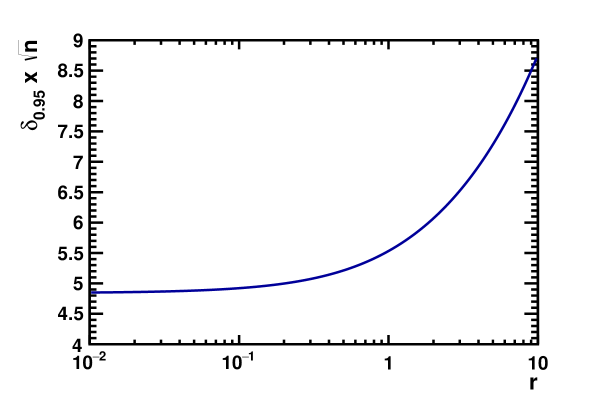
where $\sqrt{2}\,w_{\pm}=({\delta}_{0}\sqrt{s}{\pm}\sqrt{r})$ that can be used to obtain confidence regions. In particular, the value ${\delta}_{0.95}$ for the one-side 95% credible region is given by $P({\delta}{\leq}{\delta}_{0.95}|r,s)=0.95$ and its dependence with $r$ is shown in Fig. 1 assuming that ${\sigma}^{2}_{k}=4{\pi}/n;\,k=1,2,3$.

In the limit $r{\rightarrow}0$ one gets a Generalized Gamma Distribution:

$$p({\delta}|s)\,=\,s^{3/2}\,\sqrt{\frac{2}{\pi}}\,e^{\textstyle-s{\delta}^{2}/2}\,{\delta}^{2}\hskip 28.45274pt$$ (17)

with $E[{\delta}]=2\sqrt{2}/\sqrt{{\pi}s}$, $E[{\delta}^{2}]=3/s$ and the distribution function

$$P({\delta}{\leq}{\delta}_{0}|s)\,=\,\frac{2}{\sqrt{\pi}}\,{\gamma}(\frac{3}{2},\frac{s{\delta}_{0}^{2}}{2})$$ (18)

with ${\gamma}(s,x)$ the Incomplete Gamma Function.

Assuming ${\sigma}^{2}_{k}=4{\pi}/n;\,k=1,2,3$ we have, for $P({\delta}{\leq}{\delta}_{\alpha}|s)={\alpha}$, that

$$\gamma(\frac{\textstyle 3}{\textstyle 2},\frac{\textstyle{\delta}_{\alpha}^{2}\,n}{\textstyle 6})\,=\,{\alpha}\,\frac{\sqrt{\pi}}{2}$$ (19)

and, in particular, a 95% one-side credible region:

$${\delta}^{0}_{0.95}\,=\,\frac{4.84}{\sqrt{n}}$$ (20)

Within the assumptions and approximations made, this is the “smallest” 95% upper limit one may set on $\delta$ from a sample of size $n$. Moreover, from the arguments given in the previous section it is clear that, in the case of no true anisotropy, collecting data in a subset of $\Omega$ or having a non-uniform exposure time can only increase this value.

Figure 1: Upper limit at 95% CL on the dipole anisotropy parameter $\delta$ as a function of the measured parameter $r$ as defined in the text. $\delta_{0.95}$ is scaled with the factor $\sqrt{n}$, being $n$ the size of the sample.

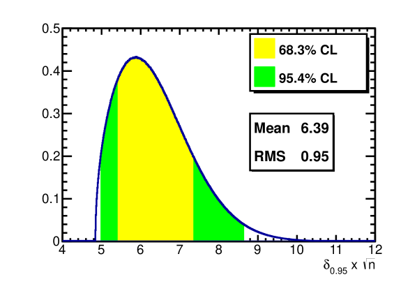
Obviously, even in the ideal case of Eqn. 3 being the true underlying distribution, this is not necessarily the limit one will get from a particular realization of the experiment. To have a feeling of what you expect for a sample of size $n$, we can evaluate $E_{r}[{\delta}_{\alpha}(r,s)]$. For ${\alpha}=0.95$ we get, under the hypothesis of no true anisotropies:

$${\delta}^{exp}_{0.95}\,=\,\frac{6.39}{\sqrt{n}}$$ (21)

The probability density function of $\delta_{0.95}$ is displayed in Fig. 2 together with the 68.3% and 95.4% equal tail area probability regions.

Figure 2: Distribution of the upper limit at 95% CL on the dipole anisotropy parameter $\delta$ expected for independent samples under the assumption of no true anisotropy. The 68.3% and 95.4% equal tail area probability regions are displayed in yellow and green respectively. $\delta_{0.95}$ is scaled with the factor $\sqrt{n}$, being $n$ the size of the sample.

4 Discussion

The conclusion from previous sections is that, under fairly general conditions, there is an absolute lower bound to the one-side confidence regions for the coefficient of anisotropy determined from a sample of events (Eqn. 20). On the other hand, the limit one may expect from a single experiment, under the assumption of no true anisotropy is given by Eqn. 21.

We have checked the consistency of these results with the published limits by the AMS and PAMELA collaborations.

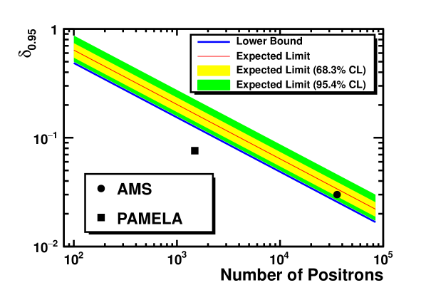
In Fig. 3, we display, as a function of the sample size, the absolute lower bound for the 95% CL exclusion limits, as well as the expected limit for a single experiment and the equal tail probability bands containing the ensemble of 68.3% and 95.4% of them under the assumption of no true anisotropy and ${\sigma}_{k}=4{\pi}/n;\,k=1,2,3$. AMS and PAMELA results are also displayed.

Figure 3: Upper limit at 95% CL on the dipole anisotropy parameter $\delta$ as a function of the number of detected positrons. The absolute lower bound (Eqn. 20) is displayed in blue. The red curve, corresponds to the expected limit for a single experiment (Eqn. 21). The equal tail probability bands containing the ensemble of 68.3% and 95.4% of the expected experimental limits are displayed in yellow and green respectively. The limit obtained by AMS [10] is shown with a circle. The result from PAMELA [11] is displayed with a square.

AMS obtained upper limits at the 95% confidence level for cumulative energy ranges on the positron over electron ratio [10]. The limit obtained for the energy range from 16 to 350 GeV on a sample of 35,000 positrons is ${\delta}_{0.95}=0.030$, in good agreement with what one may expect under the assumption of no true anisotropy ${\delta}^{exp}_{0.95}=0.034$ (Eqn. 21) and above the limit ${\delta}^{0}_{0.95}=0.026$ given by Eqn. 20.

PAMELA has recently released the search for anisotropies in cosmic-ray positrons [11]. A dipole anisotropy upper limit of ${\delta}_{0.95}=0.076$ at the 95% confidence level is determined from a data sample of 1,500 positrons selected in the rigidity range from 10 to 200 GV. This value is not consistent with the lower bound given by Eqn. 20 for this sample size (${\delta}^{0}_{0.95}=0.125$) and, therefore, we suspect that the upper bounds on the dipole anisotropy coefficient have not been derived correctly.

References

- [1] O. Adriani et al., Phys. Rev. Lett. 111 (2013) 081102; O. Adriani et al., Phys. Rev. Lett. 106 (2011) 201101.
- [2] M. Aguilar et al., Phys. Rev. Lett. 113 (2014) 121102.
- [3] O. Adriani et al., Nature 458 (2009) 607.; O. Adriani et al., Astropart. Phys. 34 (2010) 1.
- [4] M. Aguilar et al., Phys. Rev. Lett. 110 (2013) 141102; L. Accardo et al., Phys. Rev. Lett. 113 (2014) 121101.
- [5] P. Mertsch and S. Sarkar, Phys. Rev. D 90 (2014) 061301.
- [6] A. K. Harding and R. Ramaty, Proc. 20th ICRC, Moscow, USSR (1987); D. Hooper, P. Blasi and P. Serpico, J. Cosmol. Astropart. Phys. 01 (2009) 25; D. Grasso et al., Astropart. Phys. 32 (2009) 140; S. Profumo, Cent. Eur. J. Phys. 10 (2011) 1-31.
- [7] J. Silk and M. Srednicki, Phys. Rev. Lett. 53 (1984) 624; J. R. Ellis et al., Phys. Lett. B 214 (1988) 403; M. Cirelli et al., Nucl. Phys. B 813 (2009) 1.
- [8] P. Schuster et al., Phys. Rev. D 82 (2010) 115012.
- [9] S. Profumo, J. Cosmol. Astropart. Phys. 02 (2015) 1502; I. Cernuda, Astropart. Phys. 34 (2010) 59.
- [10] J. Casaus, for the AMS Collab., Proc. 33rd ICRC, Rio de Janeiro, Brazil (2013).
- [11] O. Adriani et al., Astrophys. J. 811 (2015) 21.