On the Online Frank-Wolfe Algorithms for Convex and Non-convex Optimizations

Abstract

In this paper, the online variants of the classical Frank-Wolfe algorithm are considered. We consider minimizing the regret with a stochastic cost. The online algorithms only require simple iterative updates and a non-adaptive step size rule, in contrast to the hybrid schemes commonly considered in the literature. Several new results are derived for convex and non-convex losses. With a strongly convex stochastic cost and when the optimal solution lies in the interior of the constraint set or the constraint set is a polytope, the regret bound and anytime optimality are shown to be ${\cal O}(\log^{3}T/T)$ and ${\cal O}(\log^{2}T/T)$, respectively, where $T$ is the number of rounds played. These results are based on an improved analysis on the stochastic Frank-Wolfe algorithms. Moreover, the online algorithms are shown to converge even when the loss is non-convex, i.e., the algorithms find a stationary point to the time-varying/stochastic loss at a rate of ${\cal O}(\sqrt{1/T})$. Numerical experiments on realistic data sets are presented to support our theoretical claims.

1 Introduction

Recently, Frank-Wolfe (FW) algorithm [FW56] has become popular for high-dimensional constrained optimization. Compared to the projected gradient (PG) algorithm (see [BT09, JN12a, JN12b, NJLS09]), the FW algorithm (a.k.a. conditional gradient method) is appealing due to its projection-free nature. The costly projection step in PG is replaced by a linear optimization in FW. The latter admits a closed form solution for many problems of interests in machine learning.

This work focuses on the online variants of the FW and the FW with away step (AW) algorithms. At each round, the proposed online FW/AW algorithms follow the same update equation applied in classical FW/AW and a step size is taken according to a non-adaptive rule. The only modification involved is that we use an online-computed aggregated gradient as a surrogate of the true gradient of the expected loss that we attempt to minimize. We establish fast convergence of the algorithms under various conditions.

Fast convergence for projection-free algorithms have been studied in [LJJ13, LJJ15, GH15a, GH15b, LZ14, HL16]. However, many works have considered a ‘hybrid’ approach that involves solving a regularized linear optimization during the updates [GH15b, LZ14]; or combining existing algorithms with FW [HL16]. In particular, the authors in [GH15b] showed a regret bound of ${\cal O}(\log T/T)$ for their online projection-free algorithm, where $T$ is the number of iterations, under an adversarial setting. This matches the optimal bound for strongly convex loss. The drawback of these algorithms lies on the extra complexities (in implementation and computation) added to the classical FW algorithm.

Our aim is to show that simple online projection-free methods can achieve on-the-par convergence guarantees as the sophisticated algorithms mentioned above. In particular, we present a set of new results for online FW/AW algorithms under the full information setting, i.e., complete knowledge about the loss function is retrieved at each round [ADX10] (see section 2). Our online FW algorithm is similar to the online projection-free method proposed in [HK12], while the online AW algorithm is new. For online FW algorithms, [HK12] has proven a regret of ${\cal O}(\sqrt{\log^{2}T/T})$ for convex and smooth stochastic costs. We improve the regret bound to ${\cal O}(\log^{3}T/T)$ under two different sets of assumptions: (a) the stochastic cost is strongly convex, the optimal solutions lie in the interior of ${\cal C}$ (cf. H1, for online FW); (b) ${\cal C}$ is a polytope (cf. H2, for online AW). An improved anytime optimality bound of ${\cal O}(\log^{2}T/T)$ (compared to ${\cal O}(\sqrt{\log^{2}T/T})$ in [HK12]) is also proven. We compare our results to the state-of-the-art in Table 1.

	Settings	Regret bound	Anytime bound
Garber & Hazan, 2015 [GH15b]	Hybrid algo., Lipschitz cvx. loss	${\cal O}(\sqrt{1/T})$	${\cal O}(\sqrt{\log T/T})$
	Hybrid algo., strong cvx. loss	${\cal O}(\log T/T)$	${\cal O}({\log T/T})$
Hazan & Kale, 2012 [HK12]	Simple algo., Lipschitz cvx. loss	${\cal O}(\sqrt{\log^{2}T/T})$	${\cal O}(\sqrt{\log^{2}T/T})$
	Simple algo., strong cvx. loss	${\cal O}(\sqrt{\log^{2}T/T})$	${\cal O}(\sqrt{\log^{2}T/T})$
This work	Simple algo., strong cvx. loss, interior point (online FW)	${\cal O}(\log^{3}T/T)$	${\cal O}(\log^{2}T/T)$
	Simple algo., strong cvx. loss, polytope const. (online AW)	${\cal O}(\log^{3}T/T)$	${\cal O}(\log^{2}T/T)$

Table 1: Convergence rate comparison. Note that the regret bound for [GH15b] is given under an adversarial loss setting, while the bounds for [HK12] and our work are based on a stochastic cost. Depending on the applications (see Section 5 & Appendix I), our regret and anytime bounds can be improved to ${\cal O}(\log^{2}T/T)$ and ${\cal O}(\log T/T)$, respectively.

Another interesting discovery is that the online FW/AW algorithms converge to a stationary point even when the loss is non-convex, at a rate of ${\cal O}(1/\sqrt{T})$. To the best of our knowledge, this is the first convergence rate result for non-convex online optimization with projection-free methods.

To support our claims, we perform numerical experiments on online matrix completion using realistic dataset. The proposed online schemes outperform a simple projected gradient method in terms of running time. The algorithm also demonstrates excellent performance for robust binary classification.

Related Works. In addition to the references mentioned above, this work is related to the study of stochastic optimization, e.g., [GL15, NJLS09]. [GL15] describes a FW algorithm using stochastic approximation and proves that the optimality gap converges to zero almost surely; [NJLS09] analyses the stochastic projected gradient method and proves that the convergence rate is ${\cal O}(\log t/t)$ under strong convexity and that the optimal solution lies in the interior of ${\cal C}$. This is similar to assumption H1 in this paper.

Lastly, most recent works on non-convex optimization are based on the stochastic projected gradient descent method [AZH16, GHJY15]. Projection-free non-convex optimization has only been addressed by a few authors [GL15, EV76]. At the time when we finished with the writing, we notice that several authors have published articles pertaining to offline, non-convex FW algorithm, e.g., [LJ16] achieves the same convergence rate as ours with an adaptive step size, [JLMZ16] considers a different assumption on the smoothness of loss function, [YZS14] has a slower convergence rate than ours. Nevertheless, none of the above has considered an online optimization setting with time varying objective like ours.

Notation. For any $n\in\mathbb{N}$, let $[n]$ denote the set $\{1,\cdots,n\}$. The inner product on a $n$ dimensional real Euclidian space $\mathbf{E}$ is denoted by $\langle\cdot,\cdot\rangle$ and the associated Euclidian norm by $\|\cdot\|_{2}$. The space $\mathbf{E}$ is also equipped with a norm $\|\cdot\|$ and its dual norm $\|\cdot\|_{\star}$. Diameter of the set ${\cal C}$ w.r.t. $\|\cdot\|_{\star}$ is denoted by $\rho$, that is $\textstyle\rho\mathrel{\mathop{:}}=\sup_{\theta,\theta^{\prime}\in{\cal C}}\|\theta-\theta^{\prime}\|_{\star}$. In addition, we denote the diameter of ${\cal C}$ w.r.t. the Euclidean norm as $\bar{\rho}$, i.e., $\bar{\rho}\mathrel{\mathop{:}}=\sup_{\theta,\theta^{\prime}\in{\cal C}}\|\theta-\theta^{\prime}\|_{2}$. The $i$th element in a vector ${\bm{x}}$ is denoted by $[{\bm{x}}]_{i}$.

2 Problem Setup and Algorithms

We use the setting introduced in [HK12]. The online learner wants to minimize a loss function $f$ which is the expectation of empirical loss functions $f_{t}(\bm{\theta})=f(\bm{\theta};\omega_{t})$, where $\omega_{t}$ is drawn i.i.d. from a fixed distribution ${\cal D}$: $f(\bm{\theta})\mathrel{\mathop{:}}=\mathbb{E}_{\omega\sim{\cal D}}[f(\bm{\theta};\omega)]$. The regret of a sequence of actions $\{\bm{\theta}_{t}\}_{t=1}^{T}$ is :

$$\textstyle{\cal R}_{T}\mathrel{\mathop{:}}=T^{-1}\sum_{t=1}^{T}f(\bm{\theta}_{t})-\min_{\bm{\theta}\in{\cal C}}f(\bm{\theta})\;.$$ (1)

Here, ${\cal C}$ is a bounded convex set included in $\mathbf{E}$ and $f_{t}(\cdot)$ is a continuously differentiable function.

Our proposed algorithms assume the full information setting [ADX10] such that upon playing $\bm{\theta}_{t}$, we receive full knowledge about the loss function $\bm{\theta}\mapsto f_{t}(\bm{\theta})$ . The choice of $\bm{\theta}_{t+1}$ will be based on the previously observed loss $\{f_{s}(\bm{\theta})\}_{s=1}^{t}$. Let $\gamma_{t}\in(0,1]$ be a sequence of decreasing step size (see section 3), $F_{T}(\bm{\theta})=\sum_{t=1}^{T}f_{t}(\bm{\theta})$ the aggregated loss and ${\nabla}F_{T}(\bm{\theta})$ be the gradient of $F_{t}(\bm{\theta})$ evaluated at $\bm{\theta}$, we study two online algorithms.

Online Frank-Wolfe (O-FW). The online FW algorithm, introduced in [HK12], is a direct generalization of the classical FW algorithm, as summarized in Algorithm 1. It differs from the classical FW algorithm only in the sense that the aggregated gradient ${\nabla}F_{t}(\bm{\theta}_{t})=t^{-1}\sum_{s=1}^{t}{\nabla}f_{s}(\bm{\theta}_{t})$ is used for the linear optimization in Step 4. See the comment in Remark 3 for the complexity of calculating the aggregated gradient.

Algorithm 1 Online Frank-Wolfe (O-FW).

1:  Initialize: ${{\bm{\theta}}}_{1}\leftarrow 0$

2:  for $t=1,\dots$ do

3:     Play $\bm{\theta}_{t}$ and receive $\bm{\theta}\mapsto f_{t}(\bm{\theta})$.

4:     Solve the linear optimization:

$${{\bm{a}}}_{t}\leftarrow\arg\min_{{{\bm{a}}}\in{\cal C}}~{}\big{\langle}{{\bm{a}}},{\nabla}F_{t}(\bm{\theta}_{t})\big{\rangle}\;.\vspace{-.2cm}$$ (2)

5:     Compute ${\bm{\theta}}_{t+1}\leftarrow{\bm{\theta}}_{t}+\gamma_{t}({{\bm{a}}}_{t}-{\bm{\theta}}_{t})$.

6:  end for

Algorithm 2 Online away step Frank-Wolfe (O-AW).

1:  Initialize: $n_{0}=0$, ${{\bm{\theta}}}_{1}=0$, $\mathcal{A}_{1}=\emptyset$;

2:  for $t=1,\dots$ do

3:     Play $\bm{\theta}_{t}$ and receive the loss function $\bm{\theta}\mapsto f_{t}(\bm{\theta})$ .

4:     Solve the linear optimizations with the aggregated gradient:

$${\bm{a}}_{t}^{\sf FW}\leftarrow\arg\min_{{{\bm{a}}}\in{\cal C}}~{}\big{\langle}{{\bm{a}}},{\nabla}F_{t}({\bm{\theta}}_{t})\big{\rangle},~{}{\bm{a}}_{t}^{\sf AW}\leftarrow\arg\max_{{{\bm{a}}}\in\mathcal{A}_{t}}~{}\big{\langle}{{\bm{a}}},{\nabla}F_{t}({\bm{\theta}}_{t})\big{\rangle}\vspace{-.4cm}$$ (3)

5:     if $\langle{\bm{a}}_{t}^{\sf FW}-\bm{\theta}_{t},{\nabla}F_{t}({\bm{\theta}}_{t})\rangle\leq\langle\bm{\theta}_{t}-{\bm{a}}_{t}^{\sf AW},{\nabla}F_{t}({\bm{\theta}}_{t})\rangle$ or $\mathcal{A}_{t}=\emptyset$ then

6:        FW step: ${\bm{d}}_{t}\leftarrow{\bm{a}}_{t}^{\sf FW}-\bm{\theta}_{t}$, $n_{t}\leftarrow n_{t-1}+1$, $\hat{\gamma}_{t}\leftarrow\gamma_{n_{t}}$ and $\mathcal{A}_{t+1}\leftarrow\mathcal{A}_{t}\cup\{{\bm{a}}_{t}^{\sf FW}\}$.

7:     else

8:        ${\bm{d}}_{t}\leftarrow\bm{\theta}_{t}-{\bm{a}}_{t}^{\sf AW}$, $\gamma_{\rm max}=\alpha_{t}^{{\bm{a}}_{t}^{\sf AW}}/(1-\alpha_{t}^{{\bm{a}}_{t}^{\sf AW}})$, cf. (4) for definition of $\alpha_{t}^{{\bm{a}}_{t}^{\sf AW}}$.

9:        if  $\gamma_{\rm max}\geq\gamma_{n_{t-1}}$ then

10:           AW step: $n_{t}\leftarrow n_{t-1}+1$ and $\hat{\gamma}_{t}\leftarrow\gamma_{n_{t}}$

11:        else

12:           Drop step: $\hat{\gamma}_{t}\leftarrow\gamma_{\rm max}$, $n_{t}\leftarrow n_{t-1}$ and $\mathcal{A}_{t+1}\leftarrow\mathcal{A}_{t}\setminus\{{\bm{a}}_{t}^{\sf AW}\}$

13:        end if

14:     end if

15:     Compute ${\bm{\theta}}_{t+1}\leftarrow{\bm{\theta}}_{t}+\hat{\gamma}_{t}{\bm{d}}_{t}$.

16:  end for

Online away-step Frank-Wolfe (O-AW). The online counterpart of the away step algorithm is given in Algorithm 2. By construction, the iterate $\bm{\theta}_{t}$ is a convex combination of extreme points of ${\cal C}$, referred to as active atoms. We denote by $\mathcal{A}_{t}$ the set of active atoms and denote by $\alpha_{t}^{\bm{a}}$ the positive weight of any active atom ${\bm{a}}\in\mathcal{A}_{t}$ at time $t$, that is:

$$\textstyle\bm{\theta}_{t}=\sum_{{\bm{a}}\in\mathcal{A}_{t}}\alpha_{t}^{{\bm{a}}}\cdot{\bm{a}}\quad\text{with}\quad\alpha_{t}^{\bm{a}}>0\;.$$ (4)

At each round, two types of step might be taken. If the condition of line 5 in Algorithm 2 is satisfied, we call the iteration a “FW step”, otherwise we call it an “AW step”. When a FW step is taken, a new atom ${\bm{a}}_{t}^{\sf FW}$ is selected (3), the current iterate $\bm{\theta}_{t}$ is moved towards ${\bm{a}}_{t}^{\sf FW}$ and the active set is updated accordingly (lines 6 and 15). The selected atom is the (extreme) point of ${\cal C}$ which is maximally correlated to the negative aggregated gradient. Note that this step is identical to a usual O-FW iteration. When an “AW step” is taken, a currently active atom ${\bm{a}}_{t}^{\sf AW}$ is selected (3) and the current iterate is moved away from ${\bm{a}}_{t}^{\sf AW}$ (line 8 and 15). The atom ${\bm{a}}_{t}^{\sf AW}$ is the active atom which is the most correlated to the current gradient approximation. The intuition is that taking the ‘away’ step prevents the algorithm from following a ‘zig-zag’ path when $\bm{\theta}_{t}$ is close to the boundary of ${\cal C}$ [Wol70].

Lastly, we note that the O-AW algorithm is similar to a classical AW algorithm [Wol70]. The exception is that a fixed step size rule is adopted due to the online optimization setting.

Remark 1.

As the linear optimization (3) enumerates over the active atoms ${\cal A}_{t}$ at round $t$, the O-AW algorithm is suitable when ${\cal C}$ is an atomic (or polytope) set, otherwise $|{\cal A}_{t}|$ may become too large.

Remark 2 (Linear Optimization.).

The run-time complexity of the O-FW and O-AW algorithms depends on finding efficient solution to the linear optimization step. In many cases, this is extremely efficient. For example, when ${\cal C}$ is the trace-norm ball, then the linear optimization amounts to finding the top singular vectors of the gradient; see [Jag13] for an overview.

Remark 3 (Complexity per iteration.).

In addition to the linear optimization, both O-FW/O-AW algorithms require the aggregate gradient ${\nabla}F_{t}(\bm{\theta}_{t})$ to be computed at each round, and the complexity involved grows with the round number. In cases when the loss $f_{t}$ is the negated log-likelihood of an exponential family distribution, the gradient aggregation can be replaced by an efficient ‘on-the-fly’ update, whose complexity is a dimension-dependent constant over the iterations. As demonstrated in Section 5 and Appendix I, this set-up covers many problems of interest, among others the online matrix completion and online LASSO.

3 Main Results

This section presents the main results for the convergence of O-FW/O-AW algorithms. Notice that our results for convex losses are based on an improved analysis on the stochastic/inexact invariant of FW/AW algorithms (see Anytime Analysis in subsection 3.1), while the results for non-convex losses are derived from a novel observation on the duality gap for FW algorithms. Due to space constraints, only the main results are displayed. Detailed proofs can be found in the appendices.

Some constants are defined as follows. A function $f$ is said to be $\mu$-strongly convex if, for all $\bm{\theta}$, $\tilde{\bm{\theta}}\in\mathbf{E}$,

$$f(\bm{\theta})\leq f(\tilde{\bm{\theta}})+\langle{\nabla}f(\bm{\theta}),\bm{\theta}-\tilde{\bm{\theta}}\rangle-(\mu/2)\|\bm{\theta}-\tilde{\bm{\theta}}\|_{{2}}^{2}\;.$$ (5)

We also say $f$ is $L$-smooth if for all $\bm{\theta}$, $\tilde{\bm{\theta}}\in\mathbf{E}$ we get

$$f(\tilde{\bm{\theta}})\leq f(\bm{\theta})+\langle{\nabla}f(\bm{\theta}),\tilde{\bm{\theta}}-\bm{\theta}\rangle+(L/2)\|\bm{\theta}-\tilde{\bm{\theta}}\|_{{2}}^{2}\;.$$ (6)

Lastly, $f$ is said to be $G$-Lipschitz if for all $\bm{\theta}$, $\tilde{\bm{\theta}}\in\mathbf{E}$,

$$|f(\bm{\theta})-f(\tilde{\bm{\theta}})|\leq G\|\bm{\theta}-\tilde{\bm{\theta}}\|_{*}\;.$$ (7)

3.1 Convex Loss

We analyze first Algorithm 1 and Algorithm 2 when the expected loss function $f$ is convex. In particular, our analysis will depend on the following geometric condition of the constraint set ${\cal C}$. Denote by $\partial{\cal C}$ the boundary set of ${\cal C}$. For Algorithm 1, we consider

H​​ 1.

There is a minimizer $\bm{\theta}^{\star}$ of $f$ that lies in the interior of ${\cal C}$, i.e., $\delta\mathrel{\mathop{:}}=\inf_{{\bm{s}}\in\partial{\cal C}}\|{\bm{s}}-\bm{\theta}^{\star}\|_{2}>0$.

While H1 appears to be restrictive, for Algorithm 2, we can work with a relaxed condition:

H​​ 2.

${\cal C}$ is a polytope.

As argued in [LJJ15], H2 implies that the pyramidal width for ${\cal C}$, $\delta_{\rm AW}\mathrel{\mathop{:}}=PdirW({\cal C})$, is positive; see the definition in (29) of the appendix.

Regret Analysis. Our main result is summarized as follows. For $\epsilon\in(0,1)$,

Theorem 1.

Consider O-FW (resp. O-AW). Assume H1 (resp. H2), $f(\bm{\theta})$ is $\mu$-strongly convex, $f(\bm{\theta};\omega)$ is $L$-smooth for all $\omega$ drawn from ${\cal D}$ and each element of ${\nabla}f_{t}(\bm{\theta})$ is sub-Gaussian with parameter $\sigma_{D}$. Set $\gamma_{t}=2/(t+1)$. With probability at least $1-\epsilon$ and for all $t\geq 1$, the anytime loss bounds hold:

$$\begin{split}\text{(O-FW)}&~{}~{}~{}~{}f(\bm{\theta}_{t})-\min_{\bm{\theta}\in{\cal C}}f(\bm{\theta})\leq\big{(}2\sqrt{3/2}(\sigma_{grd}\rho+L\bar{\rho}^{2})/(2\delta\sqrt{\mu})\big{)}^{2}\cdot(\log(t)\log(nt/\epsilon))\cdot t^{-1}\;,\\ \text{(O-AW)}&~{}~{}~{}~{}f(\bm{\theta}_{t})-\min_{\bm{\theta}\in{\cal C}}f(\bm{\theta})\leq\big{(}(5/3)(2\sigma_{grd}\rho+L\bar{\rho}^{2})/(\delta_{\rm AW}\sqrt{\mu})\big{)}^{2}\cdot(\log(t)\log(nt/\epsilon))\cdot t^{-1}\;,\end{split}$$ (8)

where $\sigma_{grd}={\cal O}(\max\{\sigma_{D},\bar{\rho}L\}\sqrt{n})$. Consequently, summing up the two sides of (8) from $t=1$ to $t=T$ gives the regret bound for both O-FW and O-AW:

$$\textstyle T^{-1}\sum_{t=1}^{T}f(\bm{\theta}_{t})-\min_{\bm{\theta}\in{\cal C}}f(\bm{\theta})={\cal O}(\log^{3}T/T),~{}\forall~{}T\geq 1\;.$$ (9)

Proof.

To prove Theorem 1, we first upper bound the gradient error of ${\nabla}F_{t}(\bm{\theta}_{t})$, i.e.,

Proposition 2.

Assume that $f(\bm{\theta};\omega)$ is $L$-smooth for all $\omega$ from ${\cal D}$ and each element of the vector ${\nabla}f_{t}(\bm{\theta})$ is sub-Gaussian with parameter $\sigma_{D}$. With probability at least $1-\epsilon$,

$$\|{\nabla}F_{t}(\bm{\theta}_{t})-{\nabla}f(\bm{\theta}_{t})\|_{\infty}={\cal O}(\max\{{\sigma_{D}},\bar{\rho}L\}\sqrt{n}\sqrt{{\log(t)\log(nt/\epsilon)}/{t}}),~{}\forall~{}t\geq 1\;.$$ (10)

This shows that ${\nabla}F_{t}(\bm{\theta}_{t})$ is an inexact gradient of the stochastic objective $f(\bm{\theta})$ at $\bm{\theta}_{t}$. Our proof is achieved by applying Theorem 3 (see below) by plugging in the appropriate constants. ∎

We notice that for O-FW, [HK12] has proven a regret bound of ${\cal O}(\sqrt{\log^{2}T/T})$, which is obtained by applying a uniform approximation bound on the objective value and proving a ${\cal O}(1/\sqrt{t})$ bound for the instantaneous loss $F_{t}(\bm{\theta}_{t})-F_{t}(\bm{\theta}_{t}^{\star})$. In contrast, Theorem 1 yields an improved regret by controlling the gradient error directly using Proposition 2 and analyzing O-FW/O-AW as an FW/AW algorithm with inexact gradient in the following.

Anytime Analysis. The regret analysis is derived from the following general result for FW/AW algorithms with stochastic/inexact gradients. Let $\hat{\nabla}_{t}f(\bm{\theta}_{t})$ be an estimate of $\nabla f(\bm{\theta}_{t})$ which satisfies:

H​​ 3.

For some $\alpha\in\left(0,1\right]$, $\sigma\geq 0$ and $K\in\mathbb{Z}_{+}^{\star}$. With probability at least $1-\epsilon$, we have

$$\|\hat{\nabla}_{t}f(\bm{\theta}_{t})-{\nabla}f(\bm{\theta}_{t})\|\leq\sigma(\eta^{\epsilon}_{t}/\{K+t-1\})^{\alpha},~{}\forall~{}t\geq 1\;,$$ (11)

where $\eta^{\epsilon}_{t}\geq 1$ is an increasing sequence such that the right hand side decreases to 0.

This is a more general setting than is required for the analysis of O-FW/O-AW as $\sigma,\alpha,\eta^{\epsilon}_{t}$ are arbitrary. The O-FW (or O-AW) with the above inexact gradient has the following convergence rate:

Theorem 3.

Consider the sequence $\{\bm{\theta}_{t}\}_{t=1}^{\infty}$ generated by O-FW (resp. O-AW) with the aggregated gradient ${\nabla}F_{t}(\bm{\theta}_{t})$ replaced by $\hat{\nabla}_{t}f(\bm{\theta}_{t})$ satisfying H3 with $K=2$. Assume H1 (resp. H2) and that $f(\bm{\theta})$ is $L$-smooth, $\mu$-strongly convex. Set $\gamma_{t}=2/(t+1)$. With probability at least $1-\epsilon$ and for all $t\geq 1$, we have

$$\begin{split}\text{(O-FW)}&~{}~{}~{}f(\bm{\theta}_{t})-\min_{\bm{\theta}\in{\cal C}}f(\bm{\theta})\leq\big{(}\max\{2(3/2)^{\alpha},1+2\alpha/(2-\alpha)\}(\sigma\rho+L\bar{\rho}^{2})/(2\delta\sqrt{\mu})\big{)}^{2}\cdot(\eta^{\epsilon}_{t}/(t+1))^{2\alpha}\;,\\ \text{(O-AW)}&~{}~{}~{}f(\bm{\theta}_{t})-\min_{\bm{\theta}\in{\cal C}}f(\bm{\theta})\leq 2\big{(}\max\{(3/2)^{\alpha},1+2\alpha/(2-\alpha)\}(2\sigma\rho+L\bar{\rho}^{2})/(\delta_{\rm AW}\sqrt{\mu})\big{)}^{2}\cdot(\eta^{\epsilon}_{t}/(t+1))^{2\alpha}\;,\end{split}$$ (12)

When $\alpha=0.5$, Theorem 3 improves the previous known bound of $f(\bm{\theta}_{t})-\min_{\bm{\theta}\in{\cal C}}f(\bm{\theta})={\cal O}(\sqrt{\eta^{\epsilon}_{t}/t})$ in [FG13, Jag13] under strong convexity and H1 or H2. It also matches the information-theoretical lower bound for strongly convex stochastic optimization in [RR11] (up to a log factor). Moreover, for O-AW, the strong convexity requirement on $f$ can be relaxed; see Appendix G.

3.2 Non-convex Loss

Define respectively the duality gaps for O-FW and O-AW as

$$g_{t}^{\sf FW}\mathrel{\mathop{:}}=\langle{\nabla}F_{t}(\bm{\theta}_{t}),\bm{\theta}_{t}-{\bm{a}}_{t}\rangle,~{}~{}g_{t}^{\sf AW}\mathrel{\mathop{:}}=\langle{\nabla}F_{t}(\bm{\theta}_{t}),{\bm{a}}_{t}^{\sf AW}-{\bm{a}}_{t}^{\sf FW}\rangle\;,$$ (13)

where ${\bm{a}}_{t}$ is defined in line 4 of Algorithm 1 and ${\bm{a}}_{t}^{\sf AW},{\bm{a}}_{t}^{\sf FW}$ are defined in (3) of Algorithm 2. Using the definition of ${\bm{a}}_{t}$, if $g_{t}^{\sf FW}=0$, then $\bm{\theta}_{t}$ is a stationary point to the optimization problem $\min_{\bm{\theta}\in{\cal C}}F_{t}(\bm{\theta})$. Therefore, $g_{t}^{\sf FW}$ (and similarly $g_{t}^{\sf AW}$) can be seen as a measure to the stationarity of the point $\bm{\theta}_{t}$ to the online optimization problem.

We analyze the convergence of O-FW/O-AW for general Lipschitz and smooth (possibly non-convex) loss function using the duality gaps defined above. To do so, we depart from the usual induction based proof technique (e.g., in the previous section or [Jag13, HK12]). Instead, our method of proof amounts to relate the duality gaps with a learning rate controlled by the step size rule on $\gamma_{t}$. The main result can be found below:

Theorem 4.

Consider O-FW and O-AW. Assume that each of the loss function $f_{t}$ is $G$-Lipschitz, $L$-smooth. Setting the step size sequence as $\gamma_{t}=t^{-\alpha}$ with $\alpha\in\left[0.5,1\right)$. We have

$$\begin{split}\min_{t\in[T/2+1,T]}g_{t}^{\sf FW}&\leq(1-\alpha)(4G\rho+L\bar{\rho}^{2}/2)(1-(2/3)^{1-\alpha})^{-1}\cdot T^{-(1-\alpha)},~{}\forall~{}T\geq 6\;,\\ \min_{t\in[T/2+1,T]}g_{t}^{\sf AW}&\leq(1-\alpha)(4G\rho+L\bar{\rho}^{2})(1-(4/5)^{1-\alpha})^{-1}\cdot T^{-(1-\alpha)},~{}\forall~{}T\geq 20\;.\end{split}$$ (14)

Notice that the above result is deterministic (cf. the definition of $g_{t}^{\sf FW}$, $g_{t}^{\sf AW}$) and also works with non-stochastic, non-convex losses. The above guarantees an ${\cal O}(1/T^{1-\alpha})$ rate for O-FW/O-AW at a certain round $t$ within the interval $[T/2+1,T]$. Unlike the regret/anytime analysis done previously, our bounds are stated with respect to the best duality gap attained within an interval from $t=T/2+1$ to $t=T$. This is a common artifact when analyzing the duality gap of FW [Jag13]. Furthermore, we can show that:

Proposition 5.

Consider O-FW (or O-AW), assume that each of $f_{t}$ is $G$-Lipschitz, $L$-smooth and each of ${\nabla}f_{t}(\bm{\theta})$ is sub-Gaussian with parameter $\sigma_{D}$. Set the step size sequence as $\gamma_{t}=t^{-\alpha}$ with $\alpha\in[0.5,1)$. With probability at least $1-\epsilon$ and for $T\geq 20$, there exists $t\in[T/2+1,T]$ such that

$$\max_{\bm{\theta}\in{\cal C}}~{}\langle{\nabla}f(\bm{\theta}_{t}),\bm{\theta}_{t}-\bm{\theta}\rangle={\cal O}\big{(}\max\big{\{}1/T^{1-\alpha},\sqrt{\log T/T}\big{\}}\big{)}\;.$$ (15)

The proposition indicates that the iterate $\bm{\theta}_{t}$ at round $t\in[T/2+1,T]$ is an ${\cal O}\big{(}\max\big{\{}1/T^{1-\alpha},\sqrt{\log T/T}\big{\}}\big{)}$-stationary point to the stochastic optimization $\min_{\bm{\theta}\in{\cal C}}f(\bm{\theta})$. Our proof relies on Theorem 4 and a uniform approximation bound result for ${\nabla}F_{t}(\bm{\theta}_{t})$.

4 Sketch of the Proof of Theorem 3

To provide some insights, we present the main ideas behind the proof of Theorem 3. To simplify the discussion we only consider O-FW, $K=1$, $\eta^{\epsilon}_{t}=1$ and $\alpha=0.5$ in H3. The full proof can be found in the supplementary material. Since $f(\cdot)$ is $L$-smooth and ${\cal C}$ has a diameter of $\bar{\rho}$, we have

$$f(\bm{\theta}_{t+1})\leq f(\bm{\theta}_{t})+\gamma_{t}\langle{\nabla}f(\bm{\theta}_{t}),{\bm{a}}_{t}-\bm{\theta}_{t}\rangle+\gamma_{t}^{2}L\bar{\rho}^{2}/2$$

If we define $\bm{\epsilon}_{t}\mathrel{\mathop{:}}=\hat{\nabla}_{t}f(\bm{\theta}_{t})-{\nabla}f(\bm{\theta}_{t})$, and subtract $f(\bm{\theta}^{*})$ on both sides, applying Cauchy Schwartz yields

$$h_{t+1}\leq h_{t}-\gamma_{t}g_{t}^{\sf FW}+\gamma_{t}^{2}L\bar{\rho}^{2}/2+\gamma_{t}{\rho}\|\bm{\epsilon}_{t}\|\;.$$ (16)

Observe that as $h_{t},g_{t}^{\sf FW}\geq 0$, the duality gap term $g_{t}^{\sf FW}$ determines the convergence rate of the sequence $h_{t}$ to zero.

In fact, when $f$ is convex, one can prove $g_{t}^{\sf FW}\geq h_{t}-{\rho}\|\bm{\epsilon}_{t}\|$. By the assumption H3, with probability at least $1-\epsilon$, we have

$$h_{t+1}\leq h_{t}-\gamma_{t}h_{t}+\gamma_{t}^{2}L\bar{\rho}^{2}/2+2\gamma_{t}{\rho}{\sigma}/{\sqrt{t}}=(1-\gamma_{t})h_{t}+{\cal O}(t^{-1.5})\;.$$

Setting $\gamma_{t}=1/t$ and a simple induction on the above inequality proves $h_{t}=\mathcal{O}(1/\sqrt{t})$.

An important consequence of H1 is that the latter leads to a tighter lower bound on $g_{t}^{\sf FW}$. As we present in Lemma 6 in Appendix B, under H1 and when $f$ is $\mu$-strongly convex, we can lower bound $g_{t}^{\sf FW}$ as

$$g_{t}^{\sf FW}\geq\max\{0,\delta\sqrt{\mu h_{t}}-{\rho}\|\bm{\epsilon}_{t}\|\}.$$

Note that $h_{t}$ converges to zero and the above lower bound on $g_{t}^{\sf FW}$ eventually will become tighter than the previous one, i.e., $g_{t}^{\sf FW}\geq\delta\sqrt{\mu h_{t}}-{\rho}\|\bm{\epsilon}_{t}\|\geq h_{t}-{\rho}\|\bm{\epsilon}_{t}\|$. This leads to the accelerated convergence of $h_{t}$. More formally, plugging the lower bound into (16) gives

$$h_{t+1}\leq h_{t}-\gamma_{t}\delta\sqrt{\mu h_{t}}+\gamma_{t}^{2}L\bar{\rho}^{2}/2+2\gamma_{t}{\rho}{\sigma}/{\sqrt{t}}\;.$$

Again, setting $\gamma_{t}=1/t$ and a carefully executed induction argument shows $h_{t}=\mathcal{O}(1/t)$. The same line of arguments is also used to prove the convergence rate of O-AW, where H2 will be required (instead of H1) to provide a similarly tight lower bound to $g_{t}^{\sf AW}$.

5 Numerical Experiments

We conduct numerical experiments to demonstrate the practical performance of the online algorithms. An additional experiment for online LASSO with O-AW can be found in the appendix.

5.1 Example: Online matrix completion (MC)

Consider the following setting: we are sequentially given observations in the form $(k_{t},l_{t},{Y}_{t})$, with $(k_{t},l_{t})\in[m_{1}]\times[m_{2}]$ and ${Y}_{t}\in\mathbb{R}$. The observations are assumed to be i.i.d. To define the loss function, the conditional distribution of ${Y}_{t}$ w.r.t. the sampling is parametrized by an unknown matrix $\bar{\bm{\theta}}\in\mathbb{R}^{m_{1}\times m_{2}}$ and supposed to belong to the exponential family, i.e.,

$$p_{\bar{\bm{\theta}}}({Y}_{t}|k_{t},l_{t})\mathrel{\mathop{:}}={\rm m}({Y}_{t})\exp\left({Y}_{t}\bar{\bm{\theta}}_{k_{t},l_{t}}-{\rm A}(\bar{\bm{\theta}}_{k_{t},l_{t}})\right),$$ (17)

where ${\rm m}(\cdot)$ and ${\rm A}(\cdot)$ are the base measure and log-partition functions, respectively. A natural choice for the loss function at round $t$ is obtained by taking the logarithm of the posterior, i.e.,

$$f_{t}(\bm{\theta})\mathrel{\mathop{:}}={\rm A}(\bm{\theta}_{k_{t},l_{t}})-{Y}_{t}\bm{\theta}_{k_{t},l_{t}}.$$

Our goal is to minimize the regret with a penalty favoring low rank solutions ${\cal C}\mathrel{\mathop{:}}=\{\bm{\theta}\in\mathbb{R}^{m_{1}\times m_{2}}:\|\bm{\theta}\|_{\sigma,1}\leq R\}$, and the stochastic cost associated is $f(\bm{\theta})\mathrel{\mathop{:}}=\mathbb{E}_{\bar{\bm{\theta}}}\big{[}{\rm A}(\bm{\theta}_{k_{1},l_{1}})-{Y}_{1}\bm{\theta}_{k_{1},l_{1}}\big{]}$.

Note that the aggregated gradient ${\nabla}F_{t}(\bm{\theta}_{t})=t^{-1}{\nabla}\sum_{s=1}^{t}f_{s}(\bm{\theta}_{t})$ can be expressed as:

$$\textstyle\big{[}{\nabla}F_{t}(\bm{\theta}_{t})\big{]}_{k,l}=t^{-1}{\rm A}^{\prime}([\bm{\theta}_{t}]_{k,l})\big{[}\sum_{s=1}^{t}e_{k_{s}}e_{l_{s}}^{{}^{\prime}\top}\big{]}_{k,l}-t^{-1}\big{[}\sum_{s=1}^{t}Y_{s}e_{k_{s}}e_{l_{s}}^{{}^{\prime}\top}\big{]}_{k,l},~{}\forall~{}k,l\in[m_{1}]\times[m_{2}]\;,$$

with $\{e_{k}\}_{k=1}^{m_{1}}$ (resp. $\{e^{\prime}_{l}\}_{l=1}^{m_{2}}$) the canonical basis of of $\mathbb{R}^{m_{1}}$ (resp. $\mathbb{R}^{m_{2}}$). We observe that the two matrices $\sum_{s=1}^{t}e_{k_{s}}e_{l_{s}}^{{}^{\prime}\top}$ and $\sum_{s=1}^{t}Y_{s}e_{k_{s}}e_{l_{s}}^{{}^{\prime}\top}$ can be computed ‘on-the-fly’ as the running sum. The two matrices can also be stored efficiently in the memory as they are at most $t$-sparse. The per iteration complexity is upper bounded by ${\cal O}(\min\{m_{1}m_{2},T\})$, where $T$ is the total number of observations.

We observe that for online MC, a better anytime/regret bound than the general case analyzed in Section 3 can be achieved. In particular, Appendix H shows that $\|{\nabla}F_{t}(\bm{\theta})-{\nabla}f(\bm{\theta})\|_{\sigma,\infty}={\cal O}(\sqrt{\log t/t})$. As such, the online gradient satisfies H3 with $\eta^{\epsilon}_{t}={\cal O}(\log t)$ and $\alpha=0.5$. Moreover, $f(\bm{\theta})$ is strongly convex if ${\rm A}^{\prime\prime}(\theta)\geq\mu$. For example, this holds for square loss function. Now if H1 is also satisfied, repeating the analysis in Section 3 yields an anytime and regret bound of ${\cal O}(\log t/t)$ and ${\cal O}(\log^{2}T/T)$, respectively.

We test our online MC algorithm on a small synthetically generated dataset, where $\bar{\bm{\theta}}$ is a rank-20, $200\times 5000$ matrix with Gaussian singular vectors. There are $2\times 10^{6}$ observations with Gaussian noise of variance $3$. Also, we test with two dataset movielens100k, movielens20m from [HK15], which contains $10^{5}$, $2\times 10^{7}$ movie ratings from $943$, $138493$ users on $1682$, $26744$ movies, respectively. We assume Gaussian observation and the loss function $f_{t}(\cdot)$ is designed as the square loss.

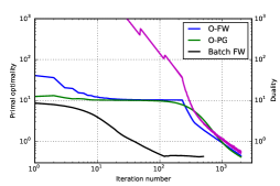
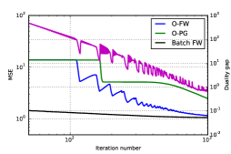
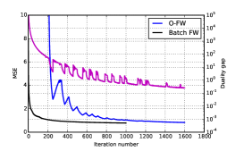
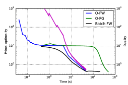
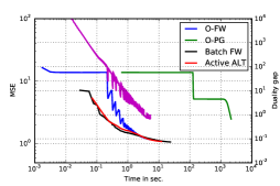
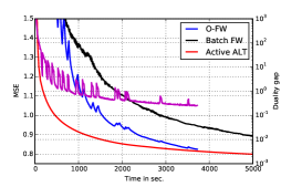
Figure 1: Online MC performance. (Left) synthetic with batch size $B=1000$; (Middle) movielens100k with $B=80$; (Right) movielens20m with $B=10000$. (Top) objective value/MSE against round number; (Bottom) against execution time. The duality gap $g_{t}^{\sf FW}$ for O-FW is plotted in purple.

Results. We compare O-FW to a simple online projected-gradient (O-PG) method. The step size for O-FW is set as $\gamma_{t}=2/(1+t)$. For the movielens datasets, the parameter $\bar{\bm{\theta}}$ is unknown, therefore we split the dataset into training ($80\%$) and testing ($20\%$) set and evaluate the mean square error on the test set. Radiuses of ${\cal C}_{R}$ are set as $R=1.1\|\bar{\bm{\theta}}\|_{\sigma,1}$ (synthetic), $R=10000$ (movielens100k) and $R=150000$ (movielens20m). Note that H1 is satisfied by the synthetic case.

The results are shown in Figure 1. For the synthetic data, we observe that the stochastic objective of O-FW decreases at a rate $\sim{\cal O}(1/t)$, as predicted in our analysis. Significant complexity reduction compared to O-PG for synthetic and movielens100k datasets are also observed. The running time is faster than the batch FW with line searched step size on movielens20m, which we suspect is caused by the simpler linear optimization (2) solved at the algorithm initialization by O-FW; and is also comparable to a state-of-the-art, specialized batch algorithm for MC problems in [HO14] (‘active ALT’) and achieves the same MSE level, even though the data are acquired in an online fashion in O-FW.

5.2 Example: Robust Binary Classification with Outliers

Consider the following online learning setting: the training data is given sequentially in the form of $(y_{t},{\bm{x}}_{t})$, where $y_{t}\in\{\pm 1\}$ is a binary label and ${\bm{x}}_{t}\in\mathbb{R}^{n}$ is a feature vector. Our goal is to train a classifier $\bm{\theta}\in\mathbb{R}^{n}$ such that for an arbitrary feature vector $\hat{\bm{x}}$ it assigns $\hat{y}={\rm sign}(\langle\bm{\theta},\hat{\bm{x}}\rangle)$.

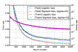
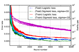
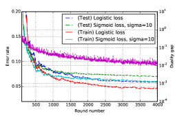
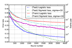
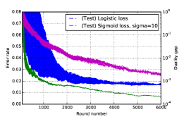
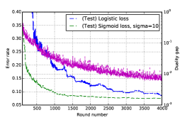
Figure 2: Binary classification performance against round number $t$ for: (Left) synthetic data; (Middle) mnist (class ‘1’); (Right) rcv1.binary. (Top) with no flip (Bottom) with $25\%$ flip in the training labels. The duality gap $g_{t}^{\sf FW}$ for O-FW with sigmoid loss is plotted in purple.

The dataset may sometimes be contaminated by wrong labels. As a remedy, we design a sigmoid loss function $f_{t}(\bm{\theta})\mathrel{\mathop{:}}=(1+{\rm exp}(10\cdot y_{t}\langle\bm{\theta},{\bm{x}}_{t}\rangle))^{-1}$ that approximates the $0/1$ loss function [SSSS11, EBG11]. Note that $f_{t}(\bm{\theta})$ is smooth and Lipschitz, but not convex. For ${\cal C}$, we consider the $\ell_{1}$ ball ${\cal C}_{\ell_{1}}=\{\bm{\theta}\in\mathbb{R}^{n}:\|\bm{\theta}\|_{1}\leq r\}$ when a sparse classifier is preferred; or the trace-norm ball ${\cal C}_{\sigma}=\{\bm{\theta}\in\mathbb{R}^{m_{1}\times m_{2}}:\|\bm{\theta}\|_{\sigma,1}\leq R\}$, where $n=m_{1}m_{2}$, when a low rank classifier is preferred.

We evaluate the performance of our online classifier on synthetic and real data. For the synthetic data, the true classifier $\bar{\bm{\theta}}$ is a rank-$10$, $30\times 30$ Gaussian matrix. Each feature ${\bm{x}}_{t}$ is a $30\times 30$ Gaussian matrix. We have $40000$ ($20000$) tuples of data for training (testing). We also test the classifier on the mnist (classifying ‘1’ from the rest of the digits), rcv1.binary dataset from LIBSVM [CL11]. The feature dimensions are $784$, $47236$, and there are $60000$ ($10000$) and $20242$ ($677399$) data tuples for training (testing), respectively. We artificially and randomly flip $0\%$, $25\%$ labels in the training set.

Results. As benchmark, we compare with the logistic loss function, i.e., $f_{t}(\bm{\theta})=\log(1+{\rm exp}(-y_{t}\langle\bm{\theta},{\bm{x}}_{t}\rangle))$. We apply O-FW with a learning rate of $\alpha=0.75$ for both loss functions, i.e., $\gamma_{t}=1/t^{0.75}$. For the synthetic data and mnist, the sigmoid (logistic) loss classifier is trained with a trace norm ball constraint of $R=1$ ($R=10$). Each round is fed with a batch of $B=10$ tuples of data. For rcv1.binary, we train the classifiers with $\ell_{1}$-ball constraint of $r=100$ ($r=1000$) for sigmoid (logistic) loss. Each round is fed with a batch of $B=5$ tuples of data.

As seen in Figure 2, the logistic loss and sigmoid loss performs similarly when there are no flip in the labels; and the sigmoid loss demonstrates better classification performance when some of the labels are flipped. Lastly, the duality gap of O-FW applied to the non-convex loss decays gradually with $t$, indicating that the algorithm converges to a stationary point.

Appendix A Proof of Proposition 2

The following proof is an application of a modified version of [SSSSS09, Theorem 5]. Let us define

$$\bm{\epsilon}_{t}(\bm{\theta})={\nabla}F_{t}(\bm{\theta})-{\nabla}f(\bm{\theta})=\frac{1}{t}\sum_{s=1}^{t}\Big{(}{\nabla}f(\bm{\theta};\omega_{s})-\mathbb{E}_{\omega\sim{\cal D}}[{\nabla}f(\bm{\theta};\omega)]\Big{)}\;.$$ (18)

From [Gau05], for some sufficiently small $\epsilon>0$, there exists a Euclidean $\epsilon$-net, $\mathcal{N}(\epsilon)$, with cardinality bounded by

$$|\mathcal{N}(\epsilon)|=\mathcal{O}\left(n^{2}\log(n)\left(\frac{\bar{\rho}}{\epsilon}\right)^{n}\right)\;.$$ (19)

In particular, for any $\bm{\theta}\in{\cal C}$ there is a point $p_{\bm{\theta}}\in\mathcal{N}(\epsilon/L)$ such that $\|p_{\bm{\theta}}-\bm{\theta}\|_{2}\leq\epsilon/L$. This implies:

$$\begin{split}\|\bm{\epsilon}_{t}(\bm{\theta})\|_{\infty}&\leq\|\bm{\epsilon}_{t}(p_{\bm{\theta}})\|_{\infty}+\|\bm{\epsilon}_{t}(p_{\bm{\theta}})-\bm{\epsilon}_{t}(\bm{\theta})\|_{\infty}\leq\|\bm{\epsilon}_{t}(p_{\bm{\theta}})\|_{\infty}+\|{\nabla}F_{t}(\bm{\theta})-{\nabla}F_{t}(p_{\bm{\theta}})\|_{\infty}+\|{\nabla}f(\bm{\theta})-{\nabla}f(p_{\bm{\theta}})\|_{\infty}\\ &\leq\|\bm{\epsilon}_{t}(p_{\bm{\theta}})\|_{\infty}+\|{\nabla}F_{t}(\bm{\theta})-{\nabla}F_{t}(p_{\bm{\theta}})\|_{2}+\|{\nabla}f(\bm{\theta})-{\nabla}f(p_{\bm{\theta}})\|_{2}\leq\|\bm{\epsilon}_{t}(p_{\bm{\theta}})\|_{\infty}+2L\|\bm{\theta}-p_{\bm{\theta}}\|_{2}\\ &\leq\|\bm{\epsilon}_{t}(p_{\bm{\theta}})\|_{\infty}+2\epsilon\;,\end{split}$$

where we used the $L$-smoothness of ${\nabla}F_{t}(\bm{\theta})$ and ${\nabla}f(\bm{\theta})$ for the second last inequality. Applying the union bound and controlling each point $p_{\bm{\theta}}\in\mathcal{N}(\epsilon/L)$ using the sub-Gaussian assumption yields:

$$\begin{split}\mathbb{P}\Big{(}\sup_{\bm{\theta}\in{\cal C}}\|\bm{\epsilon}_{t}(\bm{\theta})\|_{\infty}>s\Big{)}\leq\mathbb{P}\Big{(}\bigcup_{p_{\bm{\theta}}\in{\cal N}(\epsilon/L)}\Big{\{}\|\bm{\epsilon}_{t}(p_{\bm{\theta}})\|_{\infty}>s-2\epsilon\Big{\}}\Big{)}&\leq|\mathcal{N}(\epsilon/L)|\cdot 2n\exp\left(-\frac{t(s-2\epsilon)^{2}}{2\sigma_{D}^{2}}\right)\\ &\leq\mathcal{O}\left(n^{3}\log(n)\left(\frac{L\bar{\rho}}{\epsilon}\right)^{n}\exp\left(-\frac{t(s-2\epsilon)^{2}}{2\sigma_{D}^{2}}\right)\right)\;.\end{split}$$

Setting $s=3\epsilon$ in the above, it can be verified that the following holds with probability at least $1-\delta$

$$\|\bm{\epsilon}_{t}(\bm{\theta})\|_{\infty}={\cal O}\left(\max\{L\bar{\rho},\>\>\sigma_{D}\}\sqrt{\frac{n\log(t)\log(n/\delta)}{t}}\right)\;.$$ (20)

Applying another union bound over $t\geq 1$ (e.g., by setting $\delta=\epsilon/t^{2}$) then yields the desired result.

Appendix B Proof of Theorem 3

We define $h_{t}\mathrel{\mathop{:}}=f(\bm{\theta}_{t})-\min_{\bm{\theta}\in{\cal C}}f(\bm{\theta})$ in the following. The analysis below is done by assuming a more general step size rule $\gamma_{t}=K/(K+t-1)$ with some $K\in\mathbb{Z}_{+}^{\star}$. First of all, we notice that for both Algorithm 1 and Algorithm 2 with the step size rule $\gamma_{t}=K/(K+t-1)$, we have $\gamma_{1}=1$ and thus $h_{1}=f({\bm{a}}_{1})-f(\bm{\theta}^{\star})<\infty$. For $t\geq 2$, we have the following convergence results for FW/AW algorithms with inexact gradients.

As explained in the proof sketch, let us state the following lemma which is borrowed from [LJJ13, LJJ15].

Lemma 6.

[LJJ13, LJJ15] Assume H1 and that $f$ is $L$-smooth and $\mu$-strongly convex, then

$$\big{(}\max_{\bm{\theta}\in{\cal C}}\langle{\nabla}f(\bm{\theta}_{t}),\bm{\theta}_{t}-\bm{\theta}\rangle\big{)}^{2}\geq 2\mu\delta^{2}{h_{t}}\quad{\rm and}\quad L\bar{\rho}^{2}\geq\mu\delta^{2}\;.$$ (21)

Consider Algorithm 2, assume H2 and that $f$ is $L$-smooth and $\mu$-strongly convex, then

$$\big{(}\max_{\bm{\theta}\in{\cal A}_{t}}\langle{\nabla}f(\bm{\theta}_{t}),\bm{\theta}\rangle-\min_{\bm{\theta}\in{\cal C}}\langle{\nabla}f(\bm{\theta}_{t}),\bm{\theta}\rangle\big{)}^{2}\geq 2\mu\delta_{\rm AW}^{2}h_{t}\quad{\rm and}\quad L\bar{\rho}^{2}\geq\mu\delta_{\rm AW}^{2}\;.$$ (22)

The above lemma is a key result that leads to the linear convergence of the classical FW/AW algorithms with adaptive step sizes, as studied in [LJJ13, LJJ15]. Lemma 6 enables us to prove the theorems below for the FW/AW algorithms with inexact gradient and fixed step sizes, whose proof can be founded in Appendix E and F:

Theorem 7.

Consider Algorithm 1 with the assumptions given in Theorem 3. The following holds with probability at least $1-\epsilon$:

$$f(\bm{\theta}_{t})-f(\bm{\theta}^{\star})\leq D_{1}\left(\frac{\eta^{\epsilon}_{t}}{t+K-1}\right)^{2\alpha},~{}\forall~{}t\geq 2\;,$$ (23)

where $\beta=1+2\alpha/(K-\alpha)$ and

$$D_{1}=\max\Big{\{}4\Big{(}\frac{K+1}{K}\Big{)}^{2\alpha},\beta^{2}\Big{\}}\cdot\frac{(\rho\sigma+KL\bar{\rho}^{2}/2)^{2}}{2\delta^{2}\mu}\;.$$

The anytime bound for Algorithm 1 is obvious from the above Theorem.

Theorem 8.

Consider Algorithm 2 with the assumptions given in Theorem 3. The following holds with probability at least $1-\epsilon$:

$$f(\bm{\theta}_{t})-f(\bm{\theta}^{\star})\leq D_{2}\Big{(}\frac{\eta^{\epsilon}_{t}}{n_{t-1}+K}\Big{)}^{2\alpha},~{}\forall~{}t\geq 2,\;,$$ (24)

where $n_{t}$ is the number of non-drop steps (see Algorithm 2) up to iteration $t$, $\beta=1+2\alpha/(K-\alpha)$ and

$$D_{2}=\max\Big{\{}\Big{(}\frac{K+1}{K}\Big{)}^{2\alpha},\beta^{2}\Big{\}}\cdot\frac{2(2\rho\sigma+KL\bar{\rho}^{2}/2)^{2}}{(\delta_{\rm AW})^{2}\mu}\;.$$

In addition, we have the following Lemma for Algorithm 2.

Lemma 9.

Consider Algorithm 2. We have $n_{t}\geq t/2$ for all $t$, where $n_{t}$ is the number of non-drop steps taken until round $t$.

Proof.

Except at initialization, the active set is never empty. Indeed, if there is only one active atom left, then its weight is $1$. Therfore the condition of line 9 is satisfied and the atom cannot be dropped. Denote by $q_{t}$ the number of iterations where an atom was dropped up to time $t$ (line 12). As noted above, $n_{t}+q_{t}=t$ holds. Since to be dropped, an atom needs to be added to the active set $\mathcal{A}_{t}$ first, $q_{t}\leq t/2$ also holds, yielding the result. ∎

Combining Theorem 8 and the above lemma, we get the desirable anytime bound for Algorithm 2.

B.1 Proof of Lemma 6

We first prove the first part of the lemma, i.e., (21), pertaining to the O-FW algorithm. Let $\bar{\bm{s}}_{t}\in\partial{\cal C}$ be a point on the boundary of ${\cal C}$ such that it is co-linear with $\bm{\theta}^{\star}$ and $\bm{\theta}_{t}$. Moreover, we defin ${g}_{t}\mathrel{\mathop{:}}=\max_{\bm{\theta}\in{\cal C}}\langle{\nabla}f(\bm{\theta}_{t}),\bm{\theta}_{t}-\bm{\theta}\rangle$. As $\bm{\theta}^{\star}\in{\rm int}({\cal C})$, we can write

$$\bm{\theta}^{\star}=\bm{\theta}_{t}+\bar{\gamma}(\bar{\bm{s}}_{t}-\bm{\theta}_{t})~{}~{}~{}\text{for some}~{}~{}~{}\bar{\gamma}\in[0,1)\;.$$ (25)

From the $\mu$-strong convexity of $f$, we have

$$\frac{\mu}{2}\|\bm{\theta}^{\star}-\bm{\theta}_{t}\|_{2}^{2}\leq f(\bm{\theta}^{\star})-f(\bm{\theta}_{t})-\langle{\nabla}f(\bm{\theta}_{t}),\bm{\theta}^{\star}-\bm{\theta}_{t}\rangle=-h_{t}+\bar{\gamma}\langle{\nabla}f(\bm{\theta}_{t}),\bm{\theta}_{t}-\bar{\bm{s}}_{t}\rangle\leq-h_{t}+\bar{\gamma}g_{t}\;,$$ (26)

where the last inequality is due to the definition of $g_{t}$. Now, the left hand side of the inequality above can be bounded as

$$\frac{\mu}{2}\|\bm{\theta}^{\star}-\bm{\theta}_{t}\|_{2}^{2}=\bar{\gamma}^{2}\frac{\mu}{2}\|\bar{\bm{s}}_{t}-\bm{\theta}_{t}\|_{2}^{2}\geq\bar{\gamma}^{2}\frac{\mu}{2}\|\bar{\bm{s}}_{t}-\bm{\theta}^{\star}\|_{2}^{2}\geq\bar{\gamma}^{2}\delta^{2}\frac{\mu}{2}$$ (27)

Combining the two inequalities above yields

$$h_{t}\leq\bar{\gamma}g_{t}-\bar{\gamma}^{2}\delta^{2}\frac{\mu}{2}\leq\frac{g_{t}^{2}}{2\delta^{2}\mu}\;,$$ (28)

where the upper bound is achieved by setting $\bar{\gamma}=g_{t}/(\delta^{2}\mu)$. Recalling the definition of $g_{t}$ concludes the proof of the first part. Lastly, we note by combining Eq. (2), Remark 1 and Lemma 2 in [LJJ13], we have $L\bar{\rho}^{2}\geq\mu\delta^{2}$.

Next, we prove the second part of the lemma, i.e., (22), pertaining to the O-AW algorithm. Recall that as ${\cal C}$ is a polytope, we can write ${\cal C}={\rm conv}({\cal A})$ where ${\cal A}$ is a finite set of atoms in $\mathbb{R}^{n}$, i.e., ${\cal C}$ is a convex hull of ${\cal A}$. Note that ${\cal A}_{t}\subseteq{\cal A}$ for all $t$ in the O-AW algorithm. Let us define the pyramidal width $\delta_{\rm AW}$ of ${\cal C}$ as:

$$\delta_{\rm AW}\mathrel{\mathop{:}}=\inf_{\begin{subarray}{c}{\cal K}\in{\rm faces}({\cal C}),\bm{\theta}\in{\cal K},{\bm{d}}\in{\rm cone}({\cal C}-\bm{\theta})\setminus\{0\}\end{subarray}}\inf_{{\cal A}^{\prime}\in{\cal A}_{\bm{\theta}}}\frac{1}{\|{\bm{d}}\|_{2}}\Big{(}\max_{{\bm{y}}\in{\cal A}^{\prime}\cup\{{\bm{a}}({\cal K},{\bm{d}})\}}\langle{\bm{d}},{\bm{y}}\rangle-\min_{{\bm{y}}\in{\cal A}^{\prime}\cup\{{\bm{a}}({\cal K},{\bm{d}})\}}\langle{\bm{d}},{\bm{y}}\rangle\Big{)}\;,$$ (29)

where ${\cal A}_{\bm{\theta}}\mathrel{\mathop{:}}=\{{\cal A}^{\prime}:{\cal A}^{\prime}\subseteq{\cal A}~{}\text{such that}~{}\bm{\theta}\in{\rm conv}({\cal A}^{\prime})~{}\text{and $\bm{\theta}$ is a proper convex combination of ${\cal A}^{\prime}$}\}$ and ${\bm{a}}({\cal K},{\bm{d}})\mathrel{\mathop{:}}=\arg\max_{{\bm{v}}\in{\cal K}}\langle{\bm{v}},{\bm{d}}\rangle$. Now, define the quantities:

$$\gamma^{A}(\bm{\theta},\bm{\theta}^{\prime})\mathrel{\mathop{:}}=\frac{\langle{\nabla}f(\bm{\theta}),\bm{\theta}-\bm{\theta}^{\prime}\rangle}{\langle{\nabla}f(\bm{\theta}),{\bm{v}}_{f}(\bm{\theta})-{\bm{s}}_{f}(\bm{\theta})\rangle}\;,$$ (30)

where ${\bm{v}}_{f}(\bm{\theta})\mathrel{\mathop{:}}=\arg\min_{{\bm{a}}\in{\cal A}(\bm{\theta})}\langle{\nabla}f(\bm{\theta}),{\bm{a}}\rangle$ and ${\bm{s}}_{f}(\bm{\theta})\mathrel{\mathop{:}}=\arg\min_{{\bm{a}}\in{\cal A}}\langle{\nabla}f(\bm{\theta}),{\bm{a}}\rangle$. From [LJJ15, Theorem 6], it can be verified that

$$\mu\cdot\delta_{\rm AW}^{2}\leq\inf_{\bm{\theta}\in{\cal C}}~{}\Big{(}\inf_{\bm{\theta}^{\prime}\in{\cal C},{\rm s.t.}\langle{\nabla}f(\bm{\theta}),\bm{\theta}^{\prime}-\bm{\theta}\rangle<0}\Big{(}\frac{2}{\gamma^{A}(\bm{\theta},\bm{\theta}^{\prime})^{2}}\big{(}f(\bm{\theta}^{\prime})-f(\bm{\theta})-\langle{\nabla}f(\bm{\theta}),\bm{\theta}^{\prime}-\bm{\theta}\rangle\big{)}\Big{)}\Big{)}\;,$$ (31)

In the above, we have denoted ${\cal A}(\bm{\theta})\mathrel{\mathop{:}}=\{{\bm{v}}={\bm{v}}_{\cal A^{\prime}}(\bm{\theta})~{}:~{}{\cal A^{\prime}}\in{\cal A}_{\bm{\theta}}\}$ where ${\bm{v}}_{\cal A^{\prime}}(\bm{\theta})\mathrel{\mathop{:}}=\arg\max_{{\bm{a}}\in{\cal A}^{\prime}}\langle{\nabla}f(\bm{\theta}),{\bm{a}}\rangle$. We remark that ${\cal A}(\bm{\theta}_{t})\subseteq{\cal A}_{t}$. Note that $\gamma^{A}(\bm{\theta},\bm{\theta}^{\prime})>0$ as long as $\langle{\nabla}f(\bm{\theta}),\bm{\theta}^{\prime}-\bm{\theta}\rangle<0$ is satisfied.

Assume $\bm{\theta}_{t}\neq\bm{\theta}^{\star}$ and observe that we have $\langle{\nabla}f(\bm{\theta}_{t}),\bm{\theta}^{\star}-\bm{\theta}_{t}\rangle<0$, Eq. (31) implies that

$$\frac{\gamma^{A}(\bm{\theta}_{t},\bm{\theta}^{\star})^{2}}{2}\mu\delta_{\rm AW}^{2}\leq f(\bm{\theta}^{\star})-f(\bm{\theta}_{t})-\langle{\nabla}f(\bm{\theta}_{t}),\bm{\theta}^{\star}-\bm{\theta}_{t}\rangle=-h_{t}+\gamma^{A}(\bm{\theta}_{t},\bm{\theta}^{\star})\langle{\nabla}f(\bm{\theta}_{t}),{\bm{v}}_{f}(\bm{\theta}_{t})-{\bm{s}}_{f}(\bm{\theta}_{t})\rangle\;,$$ (32)

where the equality is found using the definition of $\gamma^{A}(\bm{\theta}_{t},\bm{\theta}^{\star})$. Define $g_{t}^{AW}\mathrel{\mathop{:}}=\max_{\bm{\theta}\in{\cal A}_{t}}\langle{\nabla}f(\bm{\theta}_{t}),\bm{\theta}\rangle-\min_{\bm{\theta}\in{\cal C}}\langle{\nabla}f(\bm{\theta}_{t}),\bm{\theta}\rangle$ and observe that

$$\langle{\nabla}f(\bm{\theta}_{t}),{\bm{s}}_{f}(\bm{\theta}_{t})\rangle=\min_{\bm{\theta}\in{\cal C}}\langle{\nabla}f(\bm{\theta}_{t}),\bm{\theta}\rangle~{}~{}~{}{\rm and}~{}~{}~{}\langle{\nabla}f(\bm{\theta}_{t}),{\bm{v}}_{f}(\bm{\theta}_{t})\rangle\leq\max_{\bm{\theta}\in{\cal A}_{t}}\langle{\nabla}f(\bm{\theta}_{t}),\bm{\theta}\rangle\;.$$ (33)

Plugging the above into (32) yields

$$h_{t}\leq-\frac{\gamma^{A}(\bm{\theta}_{t},\bm{\theta}^{\star})^{2}}{2}\mu\delta_{\rm AW}^{2}+\gamma^{A}(\bm{\theta}_{t},\bm{\theta}^{\star})g_{t}^{AW}\leq\frac{(g_{t}^{AW})^{2}}{2\delta_{\rm AW}^{2}\mu}\;,$$ (34)

where we have set $\gamma^{A}(\bm{\theta}_{t},\bm{\theta}^{\star})=g_{t}^{AW}/(\delta_{\rm AW}^{2}\mu)$ similar to the first part of this proof. This concludes the proof for the lower bound on $g_{t}^{AW}$. Lastly, it follows from Remark 7, Eq. (20) and Theorem 6 of [LJJ15] that $\mu\delta_{\rm AW}^{2}\leq L\bar{\rho}^{2}$.

Appendix C Proof of Theorem 4

In the following, we denote the minimum loss action at round $t$ as $\bm{\theta}_{t}^{\star}\in\arg\min_{\bm{\theta}\in{\cal C}}F_{t}(\bm{\theta})$. Notice that $F_{t}(\bm{\theta})$ may be non-convex.

Observe that for O-FW:

$$\begin{split}F_{t}(\bm{\theta}_{t+1})&\leq F_{t}(\bm{\theta}_{t})+\gamma_{t}\langle{\nabla}F_{t}(\bm{\theta}_{t}),{\bm{a}}_{t}-\bm{\theta}_{t}\rangle+\frac{1}{2}\gamma_{t}^{2}L\bar{\rho}^{2}=F_{t}(\bm{\theta}_{t})-\gamma_{t}g_{t}^{\sf FW}+\frac{1}{2}\gamma_{t}^{2}L\bar{\rho}^{2},\end{split}$$ (35)

where the first inequality is due to the fact that $f$ is $L$-smooth and ${\cal C}$ has a diameter of $\bar{\rho}$. Define $\Delta_{t}\mathrel{\mathop{:}}=F_{t}(\bm{\theta}_{t})-F_{t}(\bm{\theta}_{t}^{\star})$ to be the instantaneous loss at round $t$ (recall that $\bm{\theta}_{t}^{\star}\in\arg\min_{\bm{\theta}\in{\cal C}}F_{t}(\bm{\theta})$). We have

$$\begin{split}\Delta_{t+1}&=\frac{t}{t+1}\left(F_{t}(\bm{\theta}_{t+1})-F_{t}(\bm{\theta}_{t+1}^{\star})\right)+\frac{1}{t+1}(f_{t+1}(\bm{\theta}_{t+1})-f_{t+1}(\bm{\theta}_{t+1}^{\star}))\\ \end{split}$$ (36)

Note that the first part of the right hand side of (36) can be upper bounded as

$$\begin{split}F_{t}(\bm{\theta}_{t+1})-F_{t}(\bm{\theta}_{t+1}^{\star})&\leq F_{t}(\bm{\theta}_{t+1})-F_{t}(\bm{\theta}_{t}^{\star})\leq\Delta_{t}-\gamma_{t}g_{t}^{\sf FW}+\frac{1}{2}\gamma_{t}^{2}L\bar{\rho}^{2},\\ \end{split}$$ (37)

where the first inequality is due to $\bm{\theta}_{t+1}^{\star}\in{\cal C}$ and the optimality of $\bm{\theta}_{t}^{\star}$ and the second inequality is due to the $L$-smoothness of $F_{t}$. Combining (36) and (37) gives

$$\begin{split}\Delta_{t+1}&\leq\frac{t}{t+1}\left(\Delta_{t}-\gamma_{t}g_{t}^{\sf FW}+\gamma_{t}^{2}L\bar{\rho}^{2}/2\right)+\frac{1}{t+1}(f_{t+1}(\bm{\theta}_{t+1})-f_{t+1}(\bm{\theta}_{t+1}^{\star}))\\ \Longleftrightarrow\frac{t}{t+1}\gamma_{t}g_{t}^{\sf FW}&\leq\frac{t}{t+1}\left(\Delta_{t}+\frac{1}{2}\gamma_{t}^{2}L\bar{\rho}^{2}\right)+\frac{1}{t+1}(f_{t+1}(\bm{\theta}_{t+1})-f_{t+1}(\bm{\theta}_{t+1}^{\star}))-\Delta_{t+1}\;.\end{split}$$

Using the definition of $\Delta_{t+1}$, we note that $(t+1)^{-1}(f_{t+1}(\bm{\theta}_{t+1})-f_{t+1}(\bm{\theta}_{t+1}^{\star}))-\Delta_{t+1}=-(t/(t+1))(F_{t}(\bm{\theta}_{t+1})-F_{t}(\bm{\theta}_{t+1}^{\star}))$. Therefore, simplifying terms give

$$\gamma_{t}g_{t}^{\sf FW}\leq\Delta_{t}-(F_{t}(\bm{\theta}_{t+1})-F_{t}(\bm{\theta}_{t+1}^{\star}))+\gamma_{t}^{2}L\bar{\rho}^{2}/2\;.$$ (38)

Observe that:

$$\begin{split}\sum_{t=T/2+1}^{T}\Big{(}\Delta_{t}-(F_{t}(\bm{\theta}_{t+1})-F_{t}(\bm{\theta}_{t+1}^{\star}))\Big{)}&=\sum_{t=T/2+1}^{T}\Big{(}(F_{t}(\bm{\theta}_{t})-F_{t}(\bm{\theta}_{t+1}))-(F_{t}(\bm{\theta}_{t}^{\star})-F_{t}(\bm{\theta}_{t+1}^{\star}))\Big{)}\vspace{.2cm}\\ &=-F_{T}(\bm{\theta}_{T+1})+F_{T/2+1}(\bm{\theta}_{T/2+1})-F_{T/2+1}(\bm{\theta}_{T/2+1}^{\star})+F_{T}(\bm{\theta}_{T+1}^{\star})\\ &\textstyle+\sum_{t=T/2+2}^{T}t^{-1}\Big{(}f_{t}(\bm{\theta}_{t})-F_{t-1}(\bm{\theta}_{t})-(f_{t}(\bm{\theta}_{t}^{\star})-F_{t-1}(\bm{\theta}_{t}^{\star}))\Big{)}\\ &\textstyle\leq G\cdot\Big{(}\|\bm{\theta}_{T+1}-\bm{\theta}_{T+1}^{\star}\|_{*}+\|\bm{\theta}_{T/2+1}-\bm{\theta}_{T/2+1}^{\star}\|_{*}+\sum_{t=T/2+2}^{T}2t^{-1}\|\bm{\theta}_{t}-\bm{\theta}_{t}^{\star}\|_{*}\Big{)}\\ &\textstyle\leq 2\rho G\cdot\Big{(}1+\sum_{t=T/2+2}^{T}t^{-1}\Big{)}\leq 2\rho G\cdot(1+\log 2)\leq 4\rho G\;.\end{split}$$

where we have used the fact that $F_{t}(\bm{\theta}_{t})-F_{t-1}(\bm{\theta}_{t})=t^{-1}(f_{t}(\bm{\theta}_{t})-F_{t-1}(\bm{\theta}_{t}))$ in the first equality and that $f_{t},F_{t}$ are $G$-Lipschitz in the second inequality. We notice that $\sum_{t=T/2+1}^{T}\gamma_{t}^{2}=\sum_{t=T/2+1}^{T}t^{-2\alpha}\leq\log 2\leq 1$ as $\alpha\in[0.5,1]$. Summing up both side of the inequality (38) gives

$$\textstyle\Big{(}{\displaystyle\min_{t\in[T/2+1,T]}g_{t}^{\sf FW}}\Big{)}\cdot\sum_{t=T/2+1}^{T}\gamma_{t}\leq\sum_{t=T/2+1}^{T}\gamma_{t}g_{t}\leq 4\rho G+L\bar{\rho}^{2}/2\;,$$ (39)

where the inequality to the left is due to $\gamma_{t},g_{t}^{\sf FW}\geq 0$. Observe that for all $T\geq 6$, $\sum_{t=T/2+1}^{T}\gamma_{t}=\sum_{t=T/2+1}^{T}t^{-\alpha}\geq\frac{T^{1-\alpha}}{1-\alpha}\left(1-\left(\frac{2}{3}\right)^{1-\alpha}\right)=\Omega\big{(}T^{1-\alpha}\big{)}$. We conclude that

$$\min_{t\in[T/2+1,T]}g_{t}^{\sf FW}\leq\frac{1-\alpha}{T^{1-\alpha}}(4\rho G+L\bar{\rho}^{2}/2)\left(1-\left(\frac{2}{3}\right)^{1-\alpha}\right)^{-1}={\cal O}(1/T^{1-\alpha})\;.$$ (40)

For the O-AW algorithm, we observe that

$$F_{t}(\bm{\theta}_{t+1})\leq F_{t}(\bm{\theta}_{t})+\hat{\gamma}_{t}\langle{\nabla}F_{t}(\bm{\theta}_{t}),{\bm{d}}_{t}\rangle+\frac{1}{2}\hat{\gamma}_{t}^{2}L\bar{\rho}^{2}$$ (41)

Note that by construction, $\langle{\nabla}F_{t}(\bm{\theta}_{t}),{\bm{d}}_{t}\rangle=\min\{\langle{\nabla}F_{t}(\bm{\theta}_{t}),{\bm{a}}_{t}^{\sf FW}-\bm{\theta}_{t}\rangle,\langle{\nabla}F_{t}(\bm{\theta}_{t}),\bm{\theta}_{t}-{\bm{a}}_{t}^{\sf AW}\rangle\}$. Using the inequality $\min\{a,b\}\leq(1/2)(a+b)$, we have

$$F_{t}(\bm{\theta}_{t+1})\leq F_{t}(\bm{\theta}_{t})+\hat{\gamma}_{t}\Big{\langle}{\nabla}F_{t}(\bm{\theta}_{t}),\frac{1}{2}\Big{(}{\bm{a}}_{t}^{\sf FW}-{\bm{a}}_{t}^{\sf AW}\Big{)}\Big{\rangle}+\frac{1}{2}\hat{\gamma}_{t}^{2}L\bar{\rho}^{2}=F_{t}(\bm{\theta}_{t})-\frac{1}{2}\hat{\gamma}_{t}g_{t}^{\sf AW}+\frac{1}{2}\hat{\gamma}_{t}^{2}L\bar{\rho}^{2}.$$ (42)

Proceeding in a similar manner to the proof for O-FW above, we get

$$\frac{1}{2}\hat{\gamma}_{t}g_{t}^{\sf AW}\leq\Delta_{t}-(F_{t}(\bm{\theta}_{t+1})-F_{t}(\bm{\theta}_{t+1}^{\star}))+\frac{1}{2}\hat{\gamma}_{t}^{2}L\bar{\rho}^{2}.$$ (43)

The only difference from (38) in the O-FW analysis are the terms that depend on the actual step size $\hat{\gamma}_{t}$.

Now, Lemma 9 implies that at least $T/4$ non-drop steps could have taken until round $T/2$, therefore we have $\hat{\gamma}_{t}\leq\gamma_{T/4}$ for all $t\in[T/2+1,T]$ since if a non-drop step is taken, then the step size will decrease; or if a drop-step step is taken, we have $\hat{\gamma}_{t}\leq\gamma_{n_{t-1}}$ and $n_{t-1}\geq T/4$. Therefore,

$$\frac{1}{2}\sum_{t=T/2+1}^{T}\hat{\gamma}_{t}^{2}L\bar{\rho}^{2}\leq\frac{T}{4}\cdot L\bar{\rho}^{2}\Big{(}\frac{T}{4}\Big{)}^{-2\alpha}\leq L\bar{\rho}^{2}.$$

Summing the right hand side of (43) from $t=T/2+1$ to $t=T$ yields an upper bound of $4\rho G+L\bar{\rho}^{2}$.

On the other hand, define ${\cal T}_{\text{non-drop}}$ be a subset of $[T/2+1,T]$ where a non-drop step is taken. We have

$$\sum_{t=T/2+1}^{T}\hat{\gamma}_{t}\geq\sum_{t\in{\cal T}_{\text{non-drop}}}\gamma_{n_{t}}\geq\sum_{t=3T/4+1}^{T}\gamma_{t}\geq\frac{T^{1-\alpha}}{1-\alpha}\Big{(}1-\Big{(}\frac{4}{5}\Big{)}^{1-\alpha}\Big{)}=\Omega(T^{1-\alpha}),$$

where the second inequality is due to the fact that $|{\cal T}_{\text{non-drop}}|\geq T/4$ and the last inequality holds for all $T\geq 20$. Finally, summing the left hand side of (43) from $t=T/2+1$ to $t=T$ yields

$$\Big{(}\min_{t\in[T/2+1,T]}g_{t}^{\sf AW}\Big{)}\cdot\sum_{t=T/2+1}^{T}\hat{\gamma}_{t}\leq\sum_{t=T/2+1}^{T}\hat{\gamma}_{t}g_{t}^{\sf AW}\leq 4\rho G+L\bar{\rho}^{2}.$$

Therefore, we conclude that $\min_{t\in[T/2+1,T]}g_{t}^{\sf AW}={\cal O}(1/T^{1-\alpha})$ for the O-AW algorithm.

Appendix D Proof of Proposition 5

We first look at the O-FW algorithm. Our goal is to bound the following inner product

$$\max_{\bm{\theta}\in{\cal C}}\langle{\nabla}f(\bm{\theta}_{t}),\bm{\theta}_{t}-\bm{\theta}\rangle,$$

where $t\in[T/2+1,T]$ is the round index that satisfies $g_{t}^{\sf FW}={\cal O}(1/T^{1-\alpha})$, which exists due to Theorem 4. For all $\bm{\theta}\in{\cal C}$, observe that

$$\begin{split}\langle{\nabla}f(\bm{\theta}_{t}),\bm{\theta}_{t}-\bm{\theta}\rangle&\leq\langle{\nabla}F_{t}(\bm{\theta}_{t}),\bm{\theta}_{t}-\bm{\theta}\rangle+\langle{\nabla}f(\bm{\theta}_{t})-{\nabla}F_{t}(\bm{\theta}_{t}),\bm{\theta}_{t}-\bm{\theta}\rangle\\ &\leq g_{t}^{\sf FW}+\rho\|{\nabla}f(\bm{\theta}_{t})-{\nabla}F_{t}(\bm{\theta}_{t})\|.\end{split}$$ (44)

Following the same line of analysis as Proposition 2, with probability at least $1-\epsilon$, it holds that

$$\|{\nabla}f(\bm{\theta}_{t})-{\nabla}F_{t}(\bm{\theta}_{t})\|_{\infty}={\cal O}\Big{(}\max\{\sigma_{D},\bar{\rho}L\}\sqrt{\frac{n\log(t)\log(n/\epsilon)}{t}}\Big{)},$$ (45)

which is obtained from (20). Note that compared to Proposition 2, we save a factor of $\log(t)$ inside the square root as the iteration instance $t$ is fixed. Using the fact that $t\geq T/2+1$, the following holds with probability at least $1-\epsilon$,

$$\langle{\nabla}f(\bm{\theta}_{t}),\bm{\theta}_{t}-\bm{\theta}\rangle={\cal O}\big{(}\max\big{\{}1/T^{1-\alpha},\sqrt{\log T/T}\big{\}}\big{)},~{}\forall~{}\bm{\theta}\in{\cal C}.$$

For the O-AW algorithm, we observe that the inequality (42) in Appendix C can be replaced by

$$F_{t}(\bm{\theta}_{t+1})\leq F_{t}(\bm{\theta}_{t})-\hat{\gamma}_{t}\langle{\nabla}F_{t}(\bm{\theta}_{t}),\bm{\theta}_{t}-{\bm{a}}_{t}^{\sf FW}\rangle+\frac{1}{2}\hat{\gamma}_{t}^{2}L\bar{\rho}^{2}.$$

Furthermore, we can show that the inner product $\langle{\nabla}F_{t}(\bm{\theta}_{t}),\bm{\theta}_{t}-{\bm{a}}_{t}^{\sf FW}\rangle$ decays at the rate of ${\cal O}(1/T^{1-\alpha})$ by replacing $g_{t}^{\sf AW}$ in the proof in Appendix C with this inner product. Consequently, (44) holds for the $\bm{\theta}_{t}$ generated by O-AW, i.e.,

$$\langle{\nabla}f(\bm{\theta}_{t}),\bm{\theta}_{t}-\bm{\theta}\rangle\leq\langle{\nabla}F_{t}(\bm{\theta}_{t}),\bm{\theta}_{t}-{\bm{a}}_{t}^{\sf FW}\rangle+\rho\|{\nabla}f(\bm{\theta}_{t})-{\nabla}F_{t}(\bm{\theta}_{t})\|$$

Applying (45) yields our result.

Appendix E Proof of Theorem 7

This section establishes a ${\cal O}((\eta^{\epsilon}_{t}/(t+K-1))^{2\alpha})$ bound for $h_{t}$ for Algorithm 1 with inexact gradients, i.e., replacing ${\nabla}F_{t}(\bm{\theta}_{t})$ by $\hat{\nabla}_{t}f(\bm{\theta}_{t})$ satisfying H3, under the assumption that $f(\bm{\theta})$ is $L$-smooth, $\mu$-strongly convex and $\gamma_{t}=K/(K+t-1)$.

Define $\bm{\epsilon}_{t}=\hat{\nabla}_{t}f(\bm{\theta}_{t})-{\nabla}f(\bm{\theta}_{t})$, $g_{t}=\max_{{\bm{s}}\in{\cal C}}\langle\bm{\theta}_{t}-{\bm{s}},\nabla f({\bm{\theta}}_{t})\rangle$ as the duality gap at $\bm{\theta}_{t}$. Notice that (21) in Lemma 6 implies:

$${g}_{t}\geq\sqrt{2\mu\delta^{2}h_{t}},$$ (46)

Define ${\bm{s}}_{t}\in\mathop{\mathrm{arg\,max}}_{{\bm{s}}\in{\cal C}}\langle\bm{\theta}_{t}-{\bm{s}},\nabla f({\bm{\theta}}_{t})\rangle$. We note that

$$\langle\nabla f(\bm{\theta}_{t}),{{\bm{a}}}_{t}-\bm{\theta}_{t}\rangle \leq\langle\hat{\nabla}f(\bm{\theta}_{t}),{\bm{s}}_{t}-\bm{\theta}_{t}\rangle-\langle\bm{\epsilon}_{t},{{\bm{a}}}_{t}-\bm{\theta}_{t}\rangle=\langle\nabla f(\bm{\theta}_{t}),{\bm{s}}_{t}-\bm{\theta}_{t}\rangle+\langle\bm{\epsilon}_{t},{\bm{s}}_{t}-{\bm{a}}_{t}\rangle$$

$$\leq-g_{t}+\rho\|\bm{\epsilon}_{t}\|\leq-\delta\sqrt{2\mu h_{t}}+\rho\|\bm{\epsilon}_{t}\|\;,$$ (47)

where the last line follows from (46). Combining the $L$-smoothness of $f(\bm{\theta})$ and (47) yield the following with probability at least $1-\epsilon$ and for all $t\geq 1$,

$$h_{t+1}\leq\sqrt{h_{t}}(\sqrt{h_{t}}-\gamma_{t}\delta\sqrt{2\mu})+\gamma_{t}\rho\sigma\left(\frac{\eta^{\epsilon}_{t}}{t+K-1}\right)^{\alpha}+\frac{1}{2}\gamma_{t}^{2}L\bar{\rho}^{2}\;.$$ (48)

Let us recall the definition of $D_{1}$

$$D_{1}=\max\{4((K+1)/K)^{2\alpha},\beta^{2}\}(\rho\sigma+KL\bar{\rho}^{2}/2)^{2}/(2\delta^{2}\mu)\quad\text{with}\quad\beta=1+2\alpha/(K-\alpha)\;,$$ (49)

and proceed by induction. Suppose that $h_{t}\leq D_{1}(\eta^{\epsilon}_{t}/(t+K-1))^{2\alpha}$ for some $t\geq 1$. There are two cases.
Case 1 $h_{t}-\gamma_{t}\delta\sqrt{2\mu h_{t}}\leq 0$:
Then since $\gamma_{t}=K/(K+t-1)$, (48) yields

$$h_{t+1} \leq\rho\sigma K\frac{({\eta^{\epsilon}_{t}})^{\alpha}}{(K+t-1)^{1+\alpha}}+\frac{L\bar{\rho}^{2}K^{2}}{2(K+t-1)^{2}}\leq(\rho\sigma K+L\bar{\rho}^{2}K^{2}/2)\frac{(\eta^{\epsilon}_{t+1})^{2\alpha}}{(K+t-1)^{2\alpha}}$$

$$\leq(\rho\sigma K+L\bar{\rho}^{2}K^{2}/2)\Big{(}\frac{K+1}{K}\Big{)}^{2\alpha}\Big{(}\frac{\eta^{\epsilon}_{t+1}}{K+t}\Big{)}^{2\alpha}\;,$$

where we used that $\eta^{\epsilon}_{t}$ is increasing and larger than $1$. To conclude, one just needs to check that

$$(\rho\sigma K+L\bar{\rho}^{2}K^{2}/2)\Big{(}\frac{K+1}{K}\Big{)}^{2\alpha}\leq D_{1}\;.$$ (50)

Note that we have

$$D_{1}\geq\Big{(}\frac{K+1}{K}\Big{)}^{2\alpha}(\rho\sigma+L\bar{\rho}^{2}K/2)\cdot 4\frac{(\rho\sigma+L\bar{\rho}^{2}K/2)}{2\mu\delta^{2}}\geq\Big{(}\frac{K+1}{K}\Big{)}^{2\alpha}(\rho\sigma+L\bar{\rho}^{2}K/2)\cdot K\;,$$ (51)

where the last inequality is due to $L\bar{\rho}^{2}\geq\delta^{2}\mu$ from Lemma 6. Hence,

$$h_{t+1}\leq D_{1}(\eta^{\epsilon}_{t+1}/(K+t))^{2\alpha}\;.$$

Case 2 $h_{t}-\gamma_{t}\delta\sqrt{2\mu h_{t}}>0$:
By induction hypothesis and (48), we have

$$h_{t+1}-D_{1}\Big{(}\frac{\eta^{\epsilon}_{t+1}}{K+t}\Big{)}^{2\alpha}$$

$$\leq D_{1}(\Big{(}\frac{\eta^{\epsilon}_{t}}{K+t-1}\Big{)}^{2\alpha}-\Big{(}\frac{\eta^{\epsilon}_{t+1}}{K+t}\Big{)}^{2\alpha})+\frac{(\eta^{\epsilon}_{t})^{\alpha}\cdot K}{(K+t-1)^{1+\alpha}}\Big{(}\rho\sigma+L\bar{\rho}^{2}K/2-\delta\sqrt{2\mu D_{1}}\Big{)}$$

$$\leq\frac{(\eta^{\epsilon}_{t})^{\alpha}}{(K+t-1)^{1+\alpha}}\left[2\alpha D_{1}\left(\frac{\eta^{\epsilon}_{t}}{t+K-1}\right)^{\alpha}+K\rho\sigma+K^{2}L\bar{\rho}^{2}/2-\delta K\sqrt{2\mu D_{1}}\right]$$

$$\leq\frac{(\eta^{\epsilon}_{t})^{\alpha}}{(K+t-1)^{1+\alpha}}\left[2\alpha D_{1}\left(\frac{\eta^{\epsilon}_{t}}{t+K-1}\right)^{\alpha}+(K\rho\sigma+K^{2}L\bar{\rho}^{2}/2)(1-\beta)\right]$$ (52)

where we used the fact that (i) $\eta^{\epsilon}_{t}$ is increasing and larger than $1$, (ii) $t\geq 1$ and (iii) $1/(K+t-1)^{2\alpha}-1/(K+t)^{2\alpha}\leq 2\alpha/(K+t-1)^{1+2\alpha}$ in the second last inequality; and we have used the definition of $D_{1}$ in the last inequality. Define

$$t_{0}\mathrel{\mathop{:}}=\inf\{t\geq 1:2\alpha D_{1}\left(\frac{\eta^{\epsilon}_{t}}{t+K-1}\right)^{\alpha}+(K\rho\sigma+K^{2}L\bar{\rho}^{2}/2)(1-\beta)\leq 0\}.$$ (53)

Since $\eta^{\epsilon}_{t}/(K+t-1)$ is monotonically decreasing to $0$ and $\beta>1$, $t_{0}$ exists. Clearly, for any $t>t_{0}$ the RHS is non-positive. For $t\leq t_{0}$, we have

$$(K\rho\sigma+K^{2}L\bar{\rho}^{2}/2)(\beta-1)\leq 2\alpha D_{1}\left(\frac{\eta^{\epsilon}_{t}}{t+K-1}\right)^{\alpha}$$ (54)

i.e.,

$$D_{0}(K-\alpha)(\beta-1)\leq 2\alpha D_{1}\left(\frac{\eta^{\epsilon}_{t}}{t+K-1}\right)^{\alpha}$$ (55)

Hence by the definition that $\beta=1+2\alpha/(K-\alpha)$ and applying Theorem 10 (see Section E.1) we get:

$$h_{t}\leq D_{0}\left(\frac{\eta^{\epsilon}_{t}}{t+K-1}\right)^{\alpha}\leq D_{1}\left(\frac{\eta^{\epsilon}_{t}}{t+K-1}\right)^{2\alpha}$$

The initialization is easily verified as the first inequality holds true for all $t\geq 2$.

E.1 Proof of Theorem 10

Theorem 10.

Consider Algorithm 1 and assume H3 and that $f(\bm{\theta})$ is convex and $L$-smooth. Then, the following holds with probability at least $1-\epsilon$:

$$f(\bm{\theta}_{t})-f(\bm{\theta}^{\star})\leq D_{0}\left(\frac{\eta^{\epsilon}_{t}}{{t+K-1}}\right)^{\alpha},~{}\forall~{}t\geq 2\;,$$ (56)

where

$$D_{0}=\frac{K^{2}L\bar{\rho}^{2}/2+\rho\sigma K}{K-\alpha}\;.$$ (57)

Let us define $h_{t}=f(\bm{\theta}_{t})-f(\bm{\theta}^{\star})$, then we get

$$h_{t+1}\leq h_{t}+\gamma_{t}\langle\nabla f(\bm{\theta}_{t}),{{\bm{a}}}_{t}-\bm{\theta}_{t}\rangle+\frac{1}{2}\gamma_{t}^{2}L\bar{\rho}^{2}\;.$$ (58)

On the other hand, the following also hods:

$$\langle\nabla f(\bm{\theta}_{t}),{{\bm{a}}}_{t}-\bm{\theta}_{t}\rangle =\langle\hat{\nabla}f(\bm{\theta}_{t}),{{\bm{a}}}_{t}-\bm{\theta}_{t}\rangle-\langle\bm{\epsilon}_{t},{{\bm{a}}}_{t}-\bm{\theta}_{t}\rangle,$$

$$\leq\langle\hat{\nabla}f(\bm{\theta}_{t}),\bm{\theta}^{\star}-\bm{\theta}_{t}\rangle-\langle\bm{\epsilon}_{t},{{\bm{a}}}_{t}-\bm{\theta}_{t}\rangle$$

$$=\langle\nabla f(\bm{\theta}_{t}),\bm{\theta}^{\star}-\bm{\theta}_{t}\rangle+\langle\bm{\epsilon}_{t},\bm{\theta}^{\star}-{\bm{a}}_{t}\rangle$$

$$\leq-h_{t}+\rho\|\bm{\epsilon}_{t}\|\;.$$ (59)

where the second line follows from the definition of ${\bm{a}}_{t}$ and the last inequality is due to the convexity of $f$ and the definition of the diameter. Plugging (59) into (58) and using H3 yields the following with probability at least $1-\Delta$ and for all $t\geq 1$

$$h_{t+1}\leq(1-\gamma_{t})h_{t}+\gamma_{t}\rho\sigma(\frac{\eta^{\epsilon}_{t}}{K+t-1})^{\alpha}+\frac{1}{2}\gamma_{t}^{2}L\bar{\rho}^{2}\;.$$ (60)

We now proceed by induction to prove the first bound of the Theorem. Define

$$D_{0}=(K^{2}L\bar{\rho}^{2}/2+\rho\sigma K)/(K-\alpha)\;.$$

The initialization is done by applying (60) with $t=1$ and noting that $K\geq 1$. Assume that $h_{t}\leq D_{0}(\eta^{\epsilon}_{t}/(K+t-1))^{\alpha}$ for some $t\geq 1$. Since $\gamma_{t}=K/(t+K-1)$, from (60) we get:

$$h_{t+1}-D_{0}\Big{(}{\frac{\eta^{\epsilon}_{t+1}}{K+t}}\Big{)}^{\alpha}$$ (61)

$$\leq D_{0}\Big{(}\big{(}\frac{\eta^{\epsilon}_{t}}{t+K-1}\big{)}^{\alpha}-\big{(}\frac{\eta^{\epsilon}_{t+1}}{t+K}\big{)}^{\alpha}\Big{)}+\frac{K^{2}L\bar{\rho}^{2}/2+\rho\sigma K(\eta^{\epsilon}_{t})^{\alpha}-D_{0}K(\eta^{\epsilon}_{t})^{\alpha}}{(t+K-1)^{1+\alpha}}$$

$$\leq(\eta^{\epsilon}_{t})^{\alpha}\Big{(}\frac{D_{0}}{(t+K-1)^{\alpha}}-\frac{D_{0}}{(t+K)^{\alpha}}+\frac{K^{2}L\bar{\rho}^{2}/2+\rho\sigma K-D_{0}K}{(t+K-1)^{1+\alpha}}\Big{)}$$

$$\leq\frac{(\eta^{\epsilon}_{t})^{\alpha}}{(t+K-1)^{1+\alpha}}\Big{(}(\alpha-K)D_{0}+K^{2}L\bar{\rho}^{2}/2+\rho\sigma K\Big{)}\leq 0\;,$$

where we used the fact that $\eta^{\epsilon}_{t}$ is increasing and larger that $1$ for the second inequality and $1/(t+K-1)^{\alpha}-1/(t+K)^{\alpha}\leq\alpha/(t+K-1)^{1+\alpha}$ for the third inequality. The induction argument is now completed.

Appendix F Proof of Theorem 8

This section establishes a ${\cal O}((\eta^{\epsilon}_{t}/(n_{t-1}+K))^{2\alpha})$ bound for $h_{t}$ for Algorithm 2 with inexact gradients, i.e., replacing ${\nabla}F_{t}(\bm{\theta}_{t})$ by $\hat{\nabla}_{t}f(\bm{\theta}_{t})$ satisfying H3, under the assumption that $f(\bm{\theta})$ is $L$-smooth, $\mu$-strongly convex and $\gamma_{t}=K/(K+t-1)$.

Outline of the proof. Here, our strategy parallels that of Appendix E. We first show that the slow convergence rate of ${\cal O}((\eta^{\epsilon}_{t}/(n_{t-1}+K))^{\alpha})$ holds for Algorithm 2 (Theorem 11). The fast convergence rate of ${\cal O}((\eta^{\epsilon}_{t}/(n_{t-1}+K))^{2\alpha})$ is then established using induction. We have to pay special attention to the case when a drop step is taken (line 13 of Algorithm 2). In particular, when a drop step is taken, the induction step is done by Lemma 12; for otherwise, we apply similar arguments in Appendix E to proceed with the induction.

To begin our proof, let us define $\bm{\epsilon}_{t}=\hat{\nabla}_{t}f(\bm{\theta}_{t})-{\nabla}f(\bm{\theta}_{t})$,

$${\bm{b}}_{t}^{\sf FW}\mathrel{\mathop{:}}=\arg\min_{{{\bm{b}}}\in{\cal C}}~{}\big{\langle}{{\bm{b}}},{\nabla}f({\bm{\theta}}_{t})\big{\rangle},~{}{\bm{b}}_{t}^{\sf AW}\mathrel{\mathop{:}}=\arg\max_{{{\bm{b}}}\in\mathcal{A}_{t}}~{}\big{\langle}{{\bm{b}}},{\nabla}f({\bm{\theta}}_{t})\big{\rangle},~{}\bar{g}_{t}^{\sf AW}\mathrel{\mathop{:}}=\langle\nabla f(\bm{\theta}_{t}),{\bm{b}}_{t}^{\sf AW}-{\bm{b}}_{t}^{\sf FW}\rangle\;.$$

We remark that ${\bm{b}}_{t}^{\sf AW}\neq{\bm{a}}_{t}^{\sf AW}$ and ${\bm{b}}_{t}^{\sf FW}\neq{\bm{a}}_{t}^{\sf FW}$ as they are evaluated on the true gradient ${\nabla}f(\bm{\theta}_{t})$.

Recall that in Algorithm 2, we choose ${\bm{d}}_{t}$ such that $\langle\hat{\nabla}f(\bm{\theta}_{t}),{\bm{d}}_{t}\rangle=\min\{\langle\hat{\nabla}f(\bm{\theta}_{t}),{\bm{a}}_{t}^{\sf FW}-\bm{\theta}_{t}\rangle,\langle\hat{\nabla}f(\bm{\theta}_{t}),\bm{\theta}_{t}-{\bm{a}}_{t}^{\sf AW}\rangle\}$. Therefore, for $t\geq 2$:

$$\langle\hat{\nabla}f(\bm{\theta}_{t}),{\bm{d}}_{t}\rangle \leq\langle\hat{\nabla}f(\bm{\theta}_{t}),\frac{{\bm{a}}_{t}^{\sf FW}-{\bm{a}}_{t}^{\sf AW}}{2}\rangle\leq\langle\hat{\nabla}f(\bm{\theta}_{t}),\frac{{\bm{b}}_{t}^{\sf FW}-{\bm{b}}_{t}^{\sf AW}}{2}\rangle$$

$$=\langle{\nabla}f(\bm{\theta}_{t}),\frac{{\bm{b}}_{t}^{\sf FW}-{\bm{b}}_{t}^{\sf AW}}{2}\rangle+\langle\bm{\epsilon}_{t},\frac{{\bm{b}}_{t}^{\sf FW}-{\bm{b}}_{t}^{\sf AW}}{2}\rangle$$

where the second inequality is due to the definitions of ${\bm{a}}_{t}^{\sf FW}$ and ${\bm{a}}_{t}^{\sf AW}$ in (3). Hence:

$$\langle\hat{\nabla}f(\bm{\theta}_{t}),{\bm{d}}_{t}\rangle\leq-\frac{\bar{g}_{t}^{\sf AW}}{2}+\langle\bm{\epsilon}_{t},\frac{{\bm{b}}_{t}^{\sf FW}-{\bm{b}}_{t}^{\sf AW}}{2}\rangle$$ (62)

As $f$ is $L$-smooth, the following holds,

$$f(\bm{\theta}_{t+1})\leq f(\bm{\theta}_{t})+\hat{\gamma}_{t}\langle{\nabla}f(\bm{\theta}_{t}),{\bm{d}}_{t}\rangle+\frac{L\bar{\rho}^{2}}{2}\hat{\gamma}_{t}^{2}$$ (63)

$$=f(\bm{\theta}_{t})+\hat{\gamma}_{t}(\langle\hat{\nabla}f(\bm{\theta}_{t}),{\bm{d}}_{t}\rangle-\langle\bm{\epsilon}_{t},{\bm{d}}_{t}\rangle)+\hat{\gamma}_{t}^{2}\frac{L\bar{\rho}^{2}}{2}$$

$$\leq f(\bm{\theta}_{t})-\hat{\gamma}_{t}\frac{\bar{g}_{t}^{\sf AW}}{2}+\hat{\gamma}_{t}\langle\bm{\epsilon}_{t},\frac{{\bm{b}}_{t}^{\sf FW}-{\bm{b}}_{t}^{\sf AW}}{2}-{\bm{d}}_{t}\rangle+\hat{\gamma}_{t}^{2}\frac{L\bar{\rho}^{2}}{2}$$

where we used (62) for the last line. Subtracting $f(\bm{\theta}^{*})$ on both sides and applying H3 yield

$$h_{t+1}\leq h_{t}-\hat{\gamma}_{t}\frac{\bar{g}_{t}^{\sf AW}}{2}+2\hat{\gamma}_{t}\rho\sigma\left(\frac{\eta^{\epsilon}_{t}}{K+t-1}\right)^{\alpha}+\hat{\gamma}_{t}^{2}\frac{L\bar{\rho}^{2}}{2}\;,$$ (64)

where we have used $\|({\bm{b}}_{t}^{\sf FW}-{\bm{b}}_{t}^{\sf AW})/2-{\bm{d}}_{t}\|_{*}\leq 2\rho$.

We first establish a slow convergence rate of O-AW algorithm. Define

$$D_{2}^{\prime}=\frac{K}{K-\alpha}(KL\bar{\rho}^{2}/2+2\rho\sigma)\;.$$ (65)

Theorem 11.

Consider Algorithm 2. Assume H3 and that $f(\bm{\theta})$ is convex and $L$-smooth, the following holds with probablity $1-\epsilon$:

$$h_{t}\mathrel{\mathop{:}}=f(\bm{\theta}_{t})-f(\bm{\theta}^{\star})\leq D_{2}^{\prime}\Big{(}\frac{\eta^{\epsilon}_{t}}{n_{t-1}+K}\Big{)}^{\alpha}\;,$$ (66)

for all $t\geq 2$. Here $D_{2}^{\prime}$ is given in (65).

Proof.

See subsection F.1. ∎

Let us recall the definition of $D_{2}$

$$D_{2}=2\max\{((K+1)/K)^{2\alpha},\beta^{2}\}(2\rho\sigma+KL\bar{\rho}^{2}/2)^{2}/(\delta_{\rm AW}^{2}\mu)\quad\text{with}\quad\beta=1+2\alpha/(K-\alpha)\;.$$

To prove Theorem 8, we proceed by induction and assume that for some $t\geq 2$, $h_{t}\leq D_{2}(\eta^{\epsilon}_{t}/(K+n_{t-1}))^{2\alpha}$ holds. Notice that (22) in Lemma 6 gives:

$$\bar{g}_{t}^{\sf AW}\geq\sqrt{2\mu\delta_{\rm AW}^{2}h_{t}},$$ (67)

Now, suppose that $h_{t}>0$ ($h_{t}=0$ is discussed at the end of the proof). Combining (64) and (67) gives:

$$h_{t+1}\leq h_{t}-\hat{\gamma}_{t}\delta_{\rm AW}\sqrt{\frac{\mu h_{t}}{2}}+2\hat{\gamma}_{t}\rho\sigma\Big{(}\frac{\eta^{\epsilon}_{t}}{n_{t-1}+K}\Big{)}^{\alpha}+\hat{\gamma}_{t}^{2}\frac{L\bar{\rho}^{2}}{2}\;.$$ (68)

We have used the fact that $t-1\geq n_{t-1}$.

Consider two different cases. If a drop step is taken at iteration $t+1$, the induction step can be done by the following:

Lemma 12.

Suppose that $h_{t}\leq D_{2}(\eta^{\epsilon}_{t}/(K+n_{t-1}))^{2\alpha}$ and that a drop step is taken at iteration $t+1$ (see Algorithm 2 line 12), then

$$h_{t+1}\leq D_{2}\left(\frac{\eta^{\epsilon}_{t+1}}{K+n_{t}}\right)^{2\alpha}\;,$$ (69)

note that $n_{t}=n_{t-1}$ when a drop step is taken.

Proof.

See subsection F.2. ∎

The above lemma shows that the objective value does not increase when a drop step is taken.

On the other hand, when a drop step is not taken at iteration $t+1$, then from Algorithm 2, we have $\hat{\gamma}_{t}=\gamma_{n_{t}}=K/(K+n_{t}-1)$ and $n_{t}=n_{t-1}+1$. We consider the following two cases:

Case 1: If $h_{t}-\hat{\gamma}_{t}\delta_{\rm AW}\sqrt{\frac{\mu h_{t}}{2}}\leq 0$.
Then, since $\hat{\gamma}_{t}=K/(K+n_{t}-1)$ and $n_{t}\leq t$, (68) yields

$$h_{t+1} \leq 2\rho\sigma K\frac{({\eta^{\epsilon}_{t}})^{\alpha}}{(K+n_{t}-1)^{1+\alpha}}+\frac{L\bar{\rho}^{2}K^{2}}{2(K+n_{t}-1)^{2}}$$ (70)

$$\leq(2\rho\sigma K+L\bar{\rho}^{2}K^{2}/2)\frac{(\eta^{\epsilon}_{t+1})^{2\alpha}}{(K+n_{t}-1)^{2\alpha}}$$

$$\leq(2\rho\sigma K+L\bar{\rho}^{2}K^{2}/2)\Big{(}\frac{K+1}{K}\Big{)}^{2\alpha}\left(\frac{\eta^{\epsilon}_{t+1}}{K+n_{t}}\right)^{2\alpha}\;,$$

where we used that $\eta^{\epsilon}_{t}$ is increasing and larger than $1$. To conclude, one just needs to check that

$$(2\rho\sigma K+L\bar{\rho}^{2}K^{2}/2)\Big{(}\frac{K+1}{K}\Big{)}^{2\alpha}\leq D_{2}\;.$$ (71)

Note that we have

$$D_{2} \geq\Big{(}\frac{K+1}{K}\Big{)}^{2\alpha}(2\rho\sigma+L\bar{\rho}^{2}K/2)\cdot 2\frac{(2\rho\sigma+L\bar{\rho}^{2}K/2)}{\mu\delta_{\rm AW}^{2}}\geq\Big{(}\frac{K+1}{K}\Big{)}^{2\alpha}(2\rho\sigma+L\bar{\rho}^{2}K/2)\cdot K\;,$$

where the last inequality is due to $L\bar{\rho}^{2}\geq\delta_{\rm AW}^{2}\mu$ from Lemma 6. Hence,

$$h_{t+1}\leq D_{2}(\eta^{\epsilon}_{t+1}/(K+n_{t}))^{2\alpha}\;.$$

Case 2: Assume $h_{t}-\hat{\gamma}_{t}\delta_{\rm AW}\sqrt{\frac{\mu h_{t}}{2}}>0$.
By induction and (68), we have

$$h_{t+1}- D_{2}\Big{(}\frac{\eta^{\epsilon}_{t+1}}{K+n_{t}}\Big{)}^{2\alpha}$$

$$\leq D_{2}(\Big{(}\frac{\eta^{\epsilon}_{t}}{K+n_{t}-1}\Big{)}^{2\alpha}-\Big{(}\frac{\eta^{\epsilon}_{t+1}}{K+n_{t}}\Big{)}^{2\alpha})+\frac{(\eta^{\epsilon}_{t})^{\alpha}\cdot K}{(n_{t}+K-1)^{1+\alpha}}\Big{(}2\rho\sigma+C_{f}K/2-\delta_{\rm AW}\sqrt{\frac{\mu D_{2}}{2}}\Big{)}$$

$$\leq\frac{(\eta^{\epsilon}_{t})^{\alpha}}{(K+n_{t}-1)^{1+\alpha}}\big{[}2\alpha D_{2}\left(\frac{\eta^{\epsilon}_{t}}{n_{t}+K-1}\right)^{\alpha}+2K\rho\sigma+K^{2}L\bar{\rho}^{2}/2-\delta_{\rm AW}K\sqrt{\frac{\mu D_{2}}{2}}\big{]}$$

$$\leq\frac{(\eta^{\epsilon}_{t})^{\alpha}}{(K+n_{t}-1)^{1+\alpha}}\big{[}2\alpha D_{2}\left(\frac{\eta^{\epsilon}_{t}}{n_{t}+K-1}\right)^{\alpha}+(2K\rho\sigma+K^{2}L\bar{\rho}^{2}/2)(1-\beta)\big{]}$$ (72)

where we used the fact that (i) $\eta^{\epsilon}_{t}$ is increasing and larger than $1$, (ii) $t\geq 1$ and (iii) $1/(K+t-1)^{2\alpha}-1/(K+t)^{2\alpha}\leq 2\alpha/(K+t-1)^{1+2\alpha}$ in the second last inequality; and we have used the definition of $D_{2}$ in the last inequality. Define

$$t_{0}\mathrel{\mathop{:}}=\inf\{t\geq 1:2\alpha D_{2}\left(\frac{\eta^{\epsilon}_{t}}{n_{t}+K-1}\right)^{\alpha}+K(2\rho\sigma+KL\bar{\rho}^{2}/2)(1-\beta)\leq 0\}.$$ (73)

Since $\eta^{\epsilon}_{t}/(K+n_{t}-1)$ decreases to $0$ (see H3 and Lemma 9), $t_{0}$ exists. Clearly, for any $t>t_{0}$ the RHS is non-positive. For $t\leq t_{0}$, we have

$$K(2\rho\sigma+KL\bar{\rho}^{2}/2)(\beta-1)\leq 2\alpha D_{2}\left(\frac{\eta^{\epsilon}_{t}}{n_{t}+K-1}\right)^{\alpha}$$ (74)

implying

$$D_{2}^{\prime}(K-\alpha)(\beta-1)\leq 2\alpha D_{2}\left(\frac{\eta^{\epsilon}_{t}}{n_{t}+K-1}\right)^{\alpha}$$ (75)

Since $\beta=1+2\alpha/(K-\alpha)$, the left hand side of (75) equals $2\alpha D_{2}^{\prime}$ and we conclude that $D_{2}^{\prime}\leq D_{2}(\eta^{\epsilon}_{t}/(n_{t}+K-1))^{\alpha}$. Applying Theorem 11 we get:

$$h_{t}\leq D_{2}^{\prime}\left(\frac{\eta^{\epsilon}_{t}}{n_{t}+K-1}\right)^{\alpha}\leq D_{2}\left(\frac{\eta^{\epsilon}_{t}}{n_{t}+K-1}\right)^{2\alpha}$$

The induction step is completed by observing that $n_{t}-1=n_{t-1}$. The initialization is easily verified for $t=2$. If $h_{t}=0$, then by Lemma 6 yields $g_{t}^{\rm AW}=0$ and the induction is treated as Case 1.

F.1 Proof of Theorem 11

We proceed by induction and assume for some $t>0$ that $h_{t}\leq D_{2}^{\prime}(\eta^{\epsilon}_{t}/(n_{t-1}+K))^{\alpha}$ holds. First of all, observe that from the $L$-smoothness of $f(\bm{\theta})$,

$$h_{t+1}\leq h_{t}+\hat{\gamma}_{t}\langle\nabla f(\bm{\theta}_{t}),{\bm{d}}_{t}\rangle+\frac{1}{2}\hat{\gamma}_{t}^{2}L\bar{\rho}^{2}\;.$$ (76)

Moreover, we have:

$$\langle\nabla f(\bm{\theta}_{t}),{\bm{d}}_{t}\rangle =\langle\hat{\nabla}f(\bm{\theta}_{t}),{\bm{d}}_{t}\rangle-\langle\bm{\epsilon}_{t},{\bm{d}}_{t}\rangle\leq\langle\hat{\nabla}f(\bm{\theta}_{t}),{\bm{a}}_{t}^{\sf FW}-\bm{\theta}_{t}\rangle-\langle\bm{\epsilon}_{t},{\bm{d}}_{t}\rangle$$

$$\leq\langle\hat{\nabla}f(\bm{\theta}_{t}),\bm{\theta}_{\star}-\bm{\theta}_{t}\rangle-\langle\bm{\epsilon}_{t},{\bm{d}}_{t}\rangle=\langle{\nabla}f(\bm{\theta}_{t}),\bm{\theta}_{\star}-\bm{\theta}_{t}\rangle+\langle\bm{\epsilon}_{t},\bm{\theta}_{\star}-\bm{\theta}_{t}-{\bm{d}}_{t}\rangle$$

$$\leq-h_{t}+2\rho\|\bm{\epsilon}_{t}\|$$ (77)

where we used the condition of line 5 (Algorithm 2) in the first inequality and the fact $\|\bm{\theta}_{\star}-\bm{\theta}_{t}-{\bm{d}}_{t}\|_{\star}\leq 2\rho$ in the last inequality. This gives

$$h_{t+1}\leq(1-\hat{\gamma}_{t})h_{t}+2\hat{\gamma}_{t}\rho\sigma\Big{(}\frac{\eta^{\epsilon}_{t}}{K+n_{t-1}}\Big{)}^{\alpha}+\frac{1}{2}\hat{\gamma}_{t}^{2}L\bar{\rho}^{2}\;,$$ (78)

where we have used H3 and the fact that $n_{t-1}\leq t-1$.

Consider the two cases: if a drop step (line 12) is taken at iteration $t+1$, the following result that is analogous to Lemma 12 gives the induction.

Lemma 13.

Suppose that $h_{t}\leq D_{2}^{\prime}(\eta^{\epsilon}_{t}/(K+n_{t-1}))^{2\alpha}$ for $\alpha\in(0,1]$, and that a drop step is taken at time $t+1$ (see Algorithm 2 line 12), then

$$h_{t+1}\leq D_{2}^{\prime}\left(\frac{\eta^{\epsilon}_{t+1}}{K+n_{t}}\right)^{\alpha}\;.$$ (79)

Proof.

See subsection F.3. ∎

On the other hand, if a drop step is not taken, notice that we will have $\hat{\gamma}_{t}=\gamma_{n_{t}}=K/(K+n_{t}-1)$ and $n_{t}=n_{t-1}+1$. Consequently, the same induction argument in subsection E.1 (replacing $t$ by $n_{t}$ and consider $h_{t+1}-D_{2}^{\prime}(\eta^{\epsilon}_{t+1}/(K+n_{t}))^{\alpha}$) shows:

$$h_{t+1}\leq D_{2}^{\prime}\left(\frac{\eta^{\epsilon}_{t+1}}{K+n_{t}}\right)^{\alpha}.$$ (80)

The initialization of the induction is easily checked for $t=2$.

F.2 Proof of Lemma 12

Since iteration $t+1$ is a drop step, we have by construction (Algorithm 2 line 12)

$$\hat{\gamma}_{t}=\gamma_{\max}\leq\frac{K}{K+n_{t}}\quad\text{and}\quad n_{t}=n_{t-1}\;.$$

From (68) and the assumption in the lemma, we consider two cases: if $\sqrt{h_{t}}-\hat{\gamma}_{t}\sqrt{\mu\delta_{\rm AW}^{2}/2}\leq 0$, then we have

$$\begin{split}h_{t+1}-D_{2}\left(\frac{\eta^{\epsilon}_{t+1}}{K+n_{t}}\right)^{2\alpha}&\leq 2\hat{\gamma}_{t}\rho\sigma\Big{(}\frac{\eta^{\epsilon}_{t}}{n_{t-1}+K}\Big{)}^{\alpha}+\frac{1}{2}L\bar{\rho}^{2}\hat{\gamma}_{t}^{2}-D_{2}\left(\frac{\eta^{\epsilon}_{t+1}}{n_{t}+K}\right)^{2\alpha}\\ &\leq 2\rho\sigma\frac{K\cdot(\eta^{\epsilon}_{t+1})^{\alpha}}{(n_{t}+K)^{1+\alpha}}+\frac{1}{2}L\bar{\rho}^{2}\left(\frac{K}{n_{t}+K}\right)^{2}-D_{2}\left(\frac{\eta^{\epsilon}_{t+1}}{n_{t}+K}\right)^{2\alpha}\\ &\leq\left(\frac{\eta^{\epsilon}_{t+1}}{n_{t}+K}\right)^{2\alpha}\Big{(}2\rho\sigma K+K^{2}L\bar{\rho}^{2}/2-D_{2}\Big{)}\end{split}$$ (81)

The second inequality is due to $n_{t}=n_{t-1}$ and $\hat{\gamma}_{t}=\gamma_{max}\leq K/(K+n_{t})$. The last inequality is due to $2\alpha\leq\min\{2,1+\alpha\}$ for all $\alpha\in(0,1]$ and $\eta^{\epsilon}_{t}$ is an increasing sequence with $\eta^{\epsilon}_{t}\geq 1$. It can be verified that the right hand side is non-positive using the definition of $D_{2}$.

On the other hand, if $\sqrt{h_{t}}-\hat{\gamma}_{t}\sqrt{\mu\delta_{\rm AW}^{2}/2}>0$, we have from (68)

$$h_{t+1}-D_{2}\left(\frac{\eta^{\epsilon}_{t+1}}{n_{t}+K}\right)^{2\alpha}$$

$$\leq\sqrt{h_{t}}\Big{(}\sqrt{h_{t}}-\hat{\gamma}_{t}\sqrt{\mu\delta_{\rm AW}^{2}/2}\Big{)}+\frac{1}{2}L\bar{\rho}^{2}\hat{\gamma}_{t}^{2}+2\hat{\gamma}_{t}\rho\sigma\Big{(}\frac{\eta^{\epsilon}_{t}}{n_{t-1}+K}\Big{)}^{\alpha}-D_{2}\left(\frac{\eta^{\epsilon}_{t+1}}{n_{t}+K}\right)^{2\alpha}$$

$$\leq\frac{1}{2}L\bar{\rho}^{2}\hat{\gamma}_{t}^{2}+2\hat{\gamma}_{t}\rho\sigma\Big{(}\frac{\eta^{\epsilon}_{t}}{n_{t-1}+K}\Big{)}^{\alpha}-\hat{\gamma}_{t}\sqrt{D_{2}\mu\delta_{\rm AW}^{2}/2}\left(\frac{\eta^{\epsilon}_{t}}{n_{t-1}+K}\right)^{\alpha}$$

$$=\hat{\gamma}_{t}\Big{(}\frac{1}{2}L\bar{\rho}^{2}\hat{\gamma}_{t}+2\rho\sigma\Big{(}\frac{\eta^{\epsilon}_{t}}{n_{t}+K}\Big{)}^{\alpha}-\sqrt{D_{2}\mu\delta_{\rm AW}^{2}/2}\left(\frac{\eta^{\epsilon}_{t}}{n_{t}+K}\right)^{\alpha}\Big{)}$$

$$\leq\hat{\gamma}_{t}\Big{(}\frac{KL\bar{\rho}^{2}/2}{n_{t}+K}+\Big{(}2\rho\sigma-\sqrt{D_{2}\mu\delta_{\rm AW}^{2}/2}\Big{)}\left(\frac{\eta^{\epsilon}_{t}}{n_{t}+K}\right)^{\alpha}\Big{)}$$

$$\leq\hat{\gamma}_{t}\Big{(}\frac{\eta^{\epsilon}_{t}}{n_{t}+K}\Big{)}^{\alpha}\Big{(}KL\bar{\rho}^{2}/2+2\rho\sigma-\sqrt{D_{2}\mu\delta_{\rm AW}^{2}/2}\Big{)}\;.$$

The last inequality is due to $\alpha\leq 1$. Similarly, by the definition of $D_{2}$, we observe that the RHS in the above inequality is non-positive.

F.3 Proof of Lemma 13

Using (78) gives the following chain

$$\begin{split}h_{t+1}-D_{2}^{\prime}\left(\frac{\eta^{\epsilon}_{t+1}}{K+n_{t}}\right)^{\alpha}&\leq(1-\hat{\gamma}_{t})h_{t}+2\hat{\gamma}_{t}\rho\sigma\left(\frac{\eta^{\epsilon}_{t+1}}{K+n_{t}}\right)^{\alpha}+\frac{1}{2}L\bar{\rho}^{2}\hat{\gamma}_{t}^{2}-D_{2}^{\prime}\left(\frac{\eta^{\epsilon}_{t+1}}{K+n_{t}}\right)^{\alpha}\\ &\leq(1-\hat{\gamma}_{t})D_{2}^{\prime}\left(\frac{\eta^{\epsilon}_{t}}{K+n_{t}}\right)^{\alpha}+2\hat{\gamma}_{t}\rho\sigma\left(\frac{\eta^{\epsilon}_{t+1}}{K+n_{t}}\right)^{\alpha}+\frac{1}{2}L\bar{\rho}^{2}\hat{\gamma}_{t}^{2}-D_{2}^{\prime}\left(\frac{\eta^{\epsilon}_{t+1}}{K+n_{t}}\right)^{\alpha}\\ &\leq\hat{\gamma}_{t}\left((-D_{2}^{\prime}+2\rho\sigma)\left(\frac{\eta^{\epsilon}_{t}}{K+n_{t}}\right)^{\alpha}+\hat{\gamma}_{t}\frac{L\bar{\rho}^{2}}{2}\right)\\ &\leq\hat{\gamma}_{t}\left(\Big{(}-D_{2}^{\prime}+2\rho\sigma+\frac{1}{2}KL\bar{\rho}^{2}\Big{)}\left(\frac{\eta^{\epsilon}_{t}}{K+n_{t}}\right)^{\alpha}\right)\leq 0\;.\end{split}$$ (82)

In the above, the second inequality is due to $1-\hat{\gamma}_{t}\geq 0$ and the induction hypothesis; the third inequality is due to $\eta^{\epsilon}_{t}$ is increasing and; the last inequality is due to $\hat{\gamma}_{t}<K/(K+n_{t})$. The proof is completed.

Appendix G Fast convergence of O-AW without strong convexity

The proof is based on a generalization of Lemma 6, and the following result is borrowed from Theorem 11 in [LJJ15].

We focus on the anytime/regret bound studied in Section 3.1 below. In particular, the relaxed conditions for a regret bound of ${\cal O}(\log^{3}T/T)$ and anytime bound of ${\cal O}(\log^{2}t/t)$ are that (i) ${\cal C}$ is a polytope and (ii) the loss function can be written as:

$$f(\bm{\theta})=g({\bm{A}}\bm{\theta})+\langle{\bm{b}},\bm{\theta}\rangle\;.$$ (83)

where $g$ is $\mu_{g}$-strongly convex. For a general matrix ${\bm{A}}$, $f(\bm{\theta})$ may not be strongly convex.

Define ${\bm{C}}$ to be the matrix with rows containing the linear inequalities defining ${\cal C}$. Let $c_{h}$ be the Hoffman constant [LJJ15] for the matrix $[{\bm{A}};{\bm{b}}^{\top};{\bm{C}}]$, $G=\max_{\bm{\theta}\in{\cal C}}\|{\nabla}g({\bm{A}}\bm{\theta})\|$ be the maximal norm of gradient of $g$ over ${\bm{A}}{\cal C}$, $\rho_{\bm{A}}$ be the diameter of ${\bm{A}}{\cal C}$ and we define the generalized strong convexity constant:

$$\tilde{\mu}\mathrel{\mathop{:}}=\frac{1}{2c_{h}^{2}(\|{\bm{b}}\|M+3G\rho_{\bm{A}}+(2/\mu_{g})(G^{2}+1)}\;.$$ (84)

Under H2 and assuming that $h_{t}>0$ holds, applying the inequality (43) from [LJJ15] yields

$$\bar{g}_{t}^{\sf AW}\geq\delta_{AW}\sqrt{2\tilde{\mu}\cdot h_{t}}\;.$$ (85)

Subsequently, the ${\cal O}(\log^{2}T/T)$ anytime bound and ${\cal O}(\log^{3}T/T)$ regret bound in Theorem 1 can be obtained by repeating the proof in Appendix F with (85).

Appendix H Improved gradient error bound for online MC

Our goal is to show that with high probability,

$$\|{\nabla}F_{t}(\bm{\theta})-{\nabla}f(\bm{\theta})\|_{\sigma,\infty}={\cal O}(\sqrt{\log t/t}),~{}\forall~{}t~{}\text{sufficiently large}.$$ (86)

To facilitate our proof, let us state the following conditions on the observation noise statistics:

A 1.

The noise variance is finite, that is there exists a constant $\bar{\sigma}>0$ such that for all $\vartheta\in\mathbb{R}$, $0\leq{\rm A}^{\prime\prime}(\vartheta)\leq\bar{\sigma}^{2}\;,$ and the noise is sub-exponential i.e., there exist a constant $\lambda\geq 1$ such that for all $(k,l)\in[m_{1}]\times[m_{2}]$:

$$\int\exp\left(\lambda^{-1}\left|y-{\rm A}^{\prime}(\bar{\bm{\theta}}_{k,l})\right|\right)p_{\bar{\bm{\theta}}}(y|k,l)dy\leq\mathrm{e}\;,$$ (87)

where $p_{\bar{\bm{\theta}}}(\cdot)$ is defined as $p_{\bar{\bm{\theta}}}(y|k,l)\mathrel{\mathop{:}}={\rm m}(y)\exp\left(y\bar{\bm{\theta}}_{k,l}-{\rm A}(\bar{\bm{\theta}}_{k,l})\right)$ and $\mathrm{e}$ is the natural number.

A 2.

There exists a finite constant $\kappa>0$ such that for all $\bm{\theta}\in\mathcal{C}$, $k\in[m_{1}]$, $l\in[m_{2}]$

$$\kappa\geq\max\left(\sqrt{\sum_{l=1}^{m_{2}}{\rm A}^{\prime}(\bm{\theta}_{k,l})^{2}},\sqrt{\sum_{k=1}^{m_{1}}{\rm A}^{\prime}(\bm{\theta}_{k,l})^{2}}\right)\;.$$ (88)

Notice that $\kappa={\cal O}(\sqrt{\max\{m_{1},m_{2}\}})$.

We remark that A1 and A2 are satisfied by all the exponential family distributions. We also need the following proposition.

Proposition 14.

Consider a finite sequence of independent random matrices $(Z_{s})_{1\leq s\leq t}\in\mathbb{R}^{m_{1}\times m_{2}}$ satisfying $\mathbb{E}[Z_{i}]=0$. For some $U>0$, assume

$$\inf\{\lambda>0:\mathbb{E}[\exp(\|Z_{i}\|_{\sigma,\infty}/\lambda)]\leq\mathrm{e}\}\leq U\quad\forall i\in[n],$$ (89)

and there exists $\sigma_{Z}$ s.t.

$$\sigma^{2}_{Z}\geq\max\left\{\left\|\frac{1}{t}\sum_{s=1}^{t}\mathbb{E}[{Z_{s}}Z_{s}^{\top}]\right\|_{\sigma,\infty},\left\|\frac{1}{t}\sum_{s=1}^{t}\mathbb{E}[Z_{s}^{\top}Z_{s}]\right\|_{\sigma,\infty}\right\}\;.$$ (90)

Then for any $\nu>0$, with probability at least $1-\mathrm{e}^{-\nu}$

$$\left\|\frac{1}{t}\sum_{i=1}^{t}Z_{i}\right\|_{\sigma,\infty}\leq c_{U}\max\left\{\sigma_{Z}\sqrt{\frac{\nu+\log(d)}{t}},U\log(\frac{U}{\sigma_{Z}})\frac{\nu+\log(d)}{t}\right\}\;,$$ (91)

with $c_{U}$ an increasing constant with $U$.

Proof.

This result is proved in Theorem 4 in [Kol13] for symmetric matrices. Here we state a slightly different result because $\sigma^{2}_{Z}$ is an upper bound of the variance and not the variance itself. However, it does not the alter the proof and the result stays valid. This concentration is extended to rectangular matrices by dilation, see Proposition 11 in [Klo14] for details. ∎

Our result is stated as follows.

Proposition 15.

Assume A1, A2 and that the sampling distribution is uniform. Define the approximation error $\bm{\epsilon}_{t}(\bm{\theta})\mathrel{\mathop{:}}={\nabla}F_{t}(\bm{\theta})-\nabla f(\bm{\theta})$. With probability at least $1-\epsilon$, for any $t\geq T_{\epsilon}\mathrel{\mathop{:}}=(\lambda/\bar{\sigma})^{2}\log^{2}(\lambda/\bar{\sigma})\log(d+2d/\epsilon)$, and any $\bm{\theta}\in\mathcal{C}_{R}$:

$$\|\bm{\epsilon}_{t}(\bm{\theta})\|_{\sigma,\infty}=\mathcal{O}\left(c_{\lambda}\left(\kappa+\bar{\sigma}\right)\sqrt{\frac{\log(d(1+t^{2}/\epsilon))}{t(m_{1}\wedge m_{2})}}\right)\;,$$

with $\|\cdot\|_{\sigma,\infty}$ the operator norm, $c_{\lambda}$ a constant which depends only on $\lambda$. The constants $\lambda$, $\bar{\sigma}$ and $\kappa$ are defined in A1 and A2.

Proof.

For a fixed $\bm{\theta}$, by the triangle inequality

$$\|\bm{\epsilon}_{t}(\bm{\theta})\|_{\sigma,\infty}\leq\|\frac{1}{t}\sum_{s=1}^{t}{Y}_{s}e_{k_{s}}e^{{}^{\prime}\top}_{l_{s}}-\mathbb{E}[{Y}_{s}e_{k_{s}}e^{{}^{\prime}\top}_{l_{s}}]\|_{\sigma,\infty}+\|\frac{1}{t}\sum_{s=1}^{t}{\rm A}^{\prime}(\bm{\theta}_{k_{s},l_{s}})e_{k_{s}}e^{{}^{\prime}\top}_{l_{s}}-\mathbb{E}[{\rm A}^{\prime}(\bm{\theta}_{k_{s},l_{s}})e_{k_{s}}e^{{}^{\prime}\top}_{l_{s}}]\|_{\sigma,\infty}$$

Define $Z_{s}\mathrel{\mathop{:}}={Y}_{s}e_{k_{s}}e^{{}^{\prime}\top}_{l_{s}}-\mathbb{E}[{Y}_{s}e_{k_{s}}e^{{}^{\prime}\top}_{l_{s}}]$, then

$$\|\mathbb{E}[Z_{s}Z_{s}^{\top}]\|_{\sigma,\infty}\leq\|\mathbb{E}[{Y}_{s}^{2}e_{k_{s}}e^{{}^{\prime}\top}_{l_{s}}e^{{}^{\prime}}_{l_{s}}e_{k_{s}}^{\top}]\|_{\sigma,\infty}\;,$$

$$=\|\frac{1}{m_{1}m_{2}}\operatorname{diag}\left(\left(\sum_{l=1}^{m_{2}}\mathbb{E}[{Y}_{s}^{2}|k,l]\right)_{k=1}^{m_{1}}\right)\|_{\sigma,\infty}\;,$$

$$=\frac{1}{m_{1}m_{2}}\max_{k\in[m_{1}]}\left(\sum_{l=1}^{m_{2}}{\rm A}^{\prime\prime}(\bar{\bm{\theta}}_{k,l})+({\rm A}^{\prime}(\bar{\bm{\theta}}_{k,l}))^{2}\right)\;,$$

$$\leq\frac{\bar{\sigma}^{2}}{m_{1}\wedge m_{2}}+\frac{\kappa^{2}}{m_{1}m_{2}}\leq\frac{\bar{\sigma}^{2}+\kappa^{2}}{m_{1}\wedge m_{2}}\;,$$

where we used the fact that the distribution belongs to the exponential family for the second equality. Similarly one shows that $\|\mathbb{E}[Z_{s}^{\top}Z_{s}]\|_{\sigma,\infty}$ satisfies the same upper bound. Hence by Proposition 14 and A1, with probability at least $1-\mathrm{e}^{-\nu}$, it holds

$$\|\frac{1}{t}\sum_{s=1}^{t}Z_{s}\|_{\sigma,\infty}\leq c_{\lambda}\sqrt{\frac{(\bar{\sigma}^{2}+\kappa^{2})(\nu+\log(d))}{t(m_{1}\wedge m_{2})}}\;,$$ (92)

for $t$ larger than the threshold given in the proposition statement. For the second term, define $P_{t}\mathrel{\mathop{:}}=1/t\sum_{s=1}^{t}e_{k_{s}}e_{l_{s}}^{{}^{\prime}\top}-(m_{1}m_{2})^{-1}{\bm{1}\bm{1}^{\top}}$, we get

$$\begin{split}\|\frac{1}{t}\sum_{s=1}^{t}{\rm A}^{\prime}(\bm{\theta}_{k_{s},l_{s}})e_{k_{s}}e^{{}^{\prime}\top}_{l_{s}}-\mathbb{E}[{\rm A}^{\prime}(\bm{\theta}_{k_{s},l_{s}})e_{k_{s}}e^{{}^{\prime}\top}_{l_{s}}]\|_{\sigma,\infty}=\|P_{t}\odot({\rm A}^{\prime}(\bm{\theta}_{k,l}))_{k,l}\|_{\sigma,\infty}\leq\kappa\|P_{t}\|_{\sigma,\infty}\;,\end{split}$$ (93)

where $\odot$ denotes the Hardamard product and we have used Theorem 5.5.3 in [HJ94] for the last inequality. Define $Z^{\prime}_{s}\mathrel{\mathop{:}}=e_{k_{s}}e_{l_{s}}^{{}^{\prime}\top}-(m_{1}m_{2})^{-1}{\bm{1}\bm{1}^{\top}}$. Since by definition, $\lambda\geq 1$, one can again apply Proposition 14 for $U=\lambda$ and get with probability at least $1-\mathrm{e}^{-\nu}$,

$$\|P_{t}\|_{\sigma,\infty}\leq c_{\lambda}\sqrt{\frac{\nu+\log(d)}{t(m_{1}\wedge m_{2})}}\;.$$ (94)

Hence, by a union bound argument we find that with probability at least $1-2\mathrm{e}^{-\nu}$

$$\|\bm{\epsilon}_{t}\|_{\sigma,\infty}\leq c_{\lambda}\left(2\kappa+\bar{\sigma}\right)\sqrt{\frac{\nu+\log(d)}{t(m_{1}\wedge m_{2})}}\;.$$ (95)

Taking $\nu=\log(1+2t^{2}/\epsilon)$ and applying a union bound argument yields the result. ∎

Appendix I Additional results: Online LASSO

Consider the setting where we are sequentially given i.i.d. observations $({\bm{Y}}_{t},{\bm{A}}_{t})$ such that ${\bm{Y}}_{t}\in\mathbb{R}^{m}$ is the response, ${\bm{A}}_{t}\in\mathbb{R}^{m\times n}$ is the random design and

$${\bm{Y}}_{t}={\bm{A}}_{t}\bar{\bm{\theta}}+{\bm{w}}_{t}\;,$$ (96)

where the vector ${\bm{w}}_{t}$ is i.i.d., $[{\bm{w}}_{t}]_{i}$ is independent of $[{\bm{w}}_{t}]_{j}$ for $i\neq j$ and $[{\bm{w}}_{t}]_{i}$ is zero-mean and sub-Gaussian with parameter $\sigma_{w}$. We suppose that the unknown parameter $\bar{\bm{\theta}}$ is sparse. Attempting to learn $\bar{\bm{\theta}}$, a natural choice for the loss function at round $t$ is the square loss, i.e.,

$$f_{t}(\bm{\theta})=(1/2)\|{\bm{Y}}_{t}-{\bm{A}}_{t}\bm{\theta}\|_{2}^{2}$$ (97)

and the stochastic cost associated is $f(\bm{\theta})\mathrel{\mathop{:}}=\frac{1}{2}\mathbb{E}_{\bar{\bm{\theta}}}[\|{\bm{Y}}_{t}-{\bm{A}}_{t}\bm{\theta}\|_{2}^{2}]$. As $\bar{\bm{\theta}}$ is sparse, the constraint set is designed to be the $\ell_{1}$ ball, i.e., ${\cal C}=\{\bm{\theta}\in\mathbb{R}^{n}~{}:~{}\|\bm{\theta}\|_{1}\leq r\}$, where $r>0$ is a regularization constant. Note that ${\cal C}$ is a polytope.

The aggregated gradient can be expressed as

$${\nabla}F_{t}(\bm{\theta}_{t})=t^{-1}\Big{(}\sum_{s=1}^{t}{\bm{A}}_{s}^{\top}{\bm{A}}_{s}\Big{)}\bm{\theta}_{t}-t^{-1}\Big{(}\sum_{s=1}^{t}{\bm{A}}_{s}^{\top}{\bm{Y}}_{s}\Big{)}\;.$$ (98)

Similar to the case of online matrix completion, the terms $\sum_{s=1}^{t}{\bm{A}}_{s}^{\top}{\bm{A}}_{s}$ and $\sum_{s=1}^{t}{\bm{A}}_{s}^{\top}{\bm{Y}}_{s}$ can be computed ‘on-the-fly’ as running sums. Applying O-FW (Algorithm 1) or O-AW (Algorithm 2) with the above aggregated gradient yields an online LASSO algorithm with a constant complexity (dimension-dependent) per iteration. Notice that as ${\cal C}$ is an $\ell_{1}$ ball constraint, the linear optimization in Line 4 of Algorithm 1 or (3) in Algorithm 2 can be evaluated simply as ${\bm{a}}_{t}=-r\cdot{\rm sign}([{\nabla}F_{t}(\bm{\theta}_{t})]_{i})\cdot{\bm{e}}_{i}$, where $i=\arg\max_{j\in[n]}|[{\nabla}F_{t}(\bm{\theta}_{t})]_{j}|$.

Similar to the case of online MC, we derive the following ${\cal O}(\sqrt{\log t/t})$ bound for the gradient error:

Proposition 16.

Assume that $\|{\bm{A}}_{t}^{\top}{\bm{A}}_{t}-\mathbb{E}[{\bm{A}}^{\top}{\bm{A}}]\|_{max}\leq B_{1}$ and $\|{\bm{A}}_{t}\|_{max}\leq B_{2}$ almost surely, with $\|\cdot\|_{max}$ being the matrix max norm. Define $c\mathrel{\mathop{:}}=\max_{\bm{\theta}\in{\cal C}}\|\bm{\theta}-\bar{\bm{\theta}}\|_{1}$. With probability at least $1-(1+1/n)(\pi^{2}\epsilon/6)$, the following holds for all $\bm{\theta}\in{\cal C}$ and all $t\geq 1$:

$$\|{\nabla}F_{t}(\bm{\theta})-{\nabla}f(\bm{\theta})\|_{\infty}\leq(cB_{1}+\sqrt{mB_{2}\sigma_{w}^{2}})\sqrt{\frac{2(\log(2n^{2}t^{2})-\log\epsilon)}{t}}\;,$$ (99)

where $\|\cdot\|_{\infty}$ is the infinity norm and the dual norm of $\|\cdot\|_{1}$.

We observe that H3 is satisfied with $\eta^{\epsilon}_{t}$ asymptotically equivalent to $4{\log(t)}$ and $\alpha=0.5$. Furthermore, the stochastic cost $f$ is $L$-Lipschitz if $L{\bf I}\succeq\mathbb{E}[{\bm{A}}^{\top}{\bm{A}}]$; $\mu$-strongly convex if $\mathbb{E}[{\bm{A}}^{\top}{\bm{A}}]\succeq\mu{\bf 1}$ for some $\mu>0$; and H2 is satisfied as ${\cal C}$ is a polytope. The analysis from the previous section applies, i.e., O-FW/O-AW has a regret bound of ${\cal O}(\log^{2}T/T)$ and an anytime bound of ${\cal O}(\log t/t)$.

Proof.

Notice that the gradient vector is given by:

$${\nabla}f(\bm{\theta})=\mathbb{E}[{\bm{A}}^{\top}({\bm{A}}\bm{\theta}-{\bm{Y}})]=\mathbb{E}[{\bm{A}}^{\top}{\bm{A}}]\bm{\theta}-\mathbb{E}[{\bm{A}}^{\top}{\bm{Y}}].$$ (100)

We can bound the gradient estimation error as:

$$\begin{array}[]{l}\displaystyle\|{\nabla}F_{t}(\bm{\theta})-{\nabla}f(\bm{\theta})\|_{\infty}\leq\Big{\|}\frac{1}{t}\sum_{s=1}^{t}{\bm{A}}_{s}^{\top}{\bm{w}}_{s}\Big{\|}_{\infty}+\Big{\|}\frac{1}{t}\sum_{s=1}^{t}\big{(}{\bm{A}}_{s}^{\top}{\bm{A}}_{s}-\mathbb{E}[{\bm{A}}^{\top}{\bm{A}}]\big{)}(\bm{\theta}-\bar{\bm{\theta}})\Big{\|}_{\infty}\end{array}$$ (101)

To bound the second term in (101), we define ${\bm{Z}}_{s}\mathrel{\mathop{:}}={\bm{A}}_{s}^{\top}{\bm{A}}_{s}-\mathbb{E}[{\bm{A}}^{\top}{\bm{A}}]$. Observe that

$$\Big{\|}\frac{1}{t}\sum_{s=1}^{t}{\bm{Z}}_{s}(\bm{\theta}-\bar{\bm{\theta}})\Big{\|}_{\infty}=\max_{i\in[n]}\Big{|}\frac{1}{t}\sum_{s=1}^{t}{\bm{z}}_{s,i}(\bm{\theta}-\bar{\bm{\theta}})\Big{|},$$ (102)

where ${\bm{z}}_{s,i}$ denotes the $i$th row vector in ${\bm{Z}}_{s}$. Furthermore, by the Holder’s inequality,

$$\big{|}\frac{1}{t}\sum_{s=1}^{t}{\bm{z}}_{s,i}(\bm{\theta}-\bar{\bm{\theta}})\big{|}\leq\|\bm{\theta}-\bar{\bm{\theta}}\|_{1}\big{\|}\frac{1}{t}\sum_{s=1}^{t}{\bm{z}}_{s,i}\big{\|}_{\infty},$$ (103)

Now that ${\bm{z}}_{s,i}$ is a zero-mean, independent random vector with elements bounded in $[-B_{1},B_{1}]$, applying the union bound and the Hoefding’s inequality gives:

$$\mathbb{P}\big{(}\big{\|}\textstyle(1/t)\sum_{s=1}^{t}{\bm{z}}_{s,i}\big{\|}_{\infty}\geq x,~{}\forall~{}i\big{)}\leq 2n^{2}\mathrm{e}^{-\frac{x^{2}t}{2B_{1}^{2}}}.$$ (104)

Setting $x=B_{1}\sqrt{2(\log(2n^{2}t^{2})-\log\epsilon)/t}$ gives $\epsilon/t^{2}$ on the right hand side. With probability at least $1-\epsilon/t^{2}$, we have

$$\Big{\|}\frac{1}{t}\sum_{s=1}^{t}{\bm{Z}}_{s}\bm{\theta}\Big{\|}_{\infty}\leq cB_{1}\sqrt{2(\log(2n^{2}t^{2})-\log\Delta)/t},$$ (105)

To bound the first term in (101), we find that the $i$th element of the vector ${\bm{A}}_{s}^{\top}{\bm{w}}_{s}$ is zero-mean. Furthermore, it can be verified that

$$\mathbb{E}\big{[}\mathrm{e}^{\big{(}\lambda\sum_{j=1}^{m}A_{s,i,j}w_{s,j}\big{)}}\big{]}\leq\mathrm{e}^{\lambda^{2}\cdot m\sigma_{w}^{2}B_{2}/2},$$ (106)

for all $\lambda\in\mathbb{R}$, where $A_{s,i,j}$ is the $(i,j)$th element of ${\bm{A}}_{s}$ and $w_{s,j}$ is the $j$th element of ${\bm{w}}_{s}$. In other words, the $i$th element of ${\bm{A}}_{s}^{\top}{\bm{w}}_{s}$ is sub-Gaussian with parameter $m\cdot\sigma_{w}^{2}B_{2}$. It follows by the Hoefding’s inequality that

$$\mathbb{P}\big{(}\big{\|}\frac{1}{t}\sum_{s=1}^{t}{\bm{A}}_{s}^{\top}{\bm{w}}_{s}\big{\|}_{\infty}\geq x\big{)}\leq 2n\mathrm{e}^{-\frac{x^{2}t}{2mB_{2}\sigma_{w}^{2}}}.$$ (107)

Setting $x=\sigma_{w}\sqrt{2mB_{2}(\log(2n^{2}t^{2})-\log\epsilon)/t}$ yields $\epsilon/(nt^{2})$ on the right hand side. Combining (104), (107) and using a union bound argument (for all $t\geq 1$) yields the desired result. ∎

I.1 Numerical Result

We present numerical results on both synthetic data and realistic data.

Synthetic Data. We set ${\bm{A}}_{t}={\bm{A}}$ as fixed for all $t$ with dimension $80\times 300$ and the parameter $\bar{\bm{\theta}}\in\mathbb{R}^{300}$ is a vector with $10\%$ sparsity and independent ${\cal N}(0,1)$ elements. We also set $\sigma_{w}=10$. The matrix ${\bm{A}}$ is generated as a random Gaussian matrix with independent ${\cal N}(0,1)$ elements. For benchmarking purpose, we have compared the O-FW/O-AW’s performance with a stochastic projected gradient (sPG) method [RVV14] with a fixed step size $1/L$.

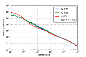
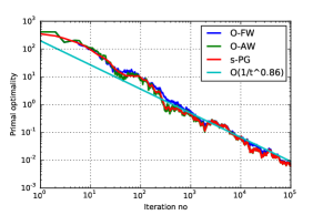
Figure 3: Online LASSO with synthetic data. Convergence of the primal optimality for online LASSO with (Left) $r=1.1\|\bar{\bm{\theta}}\|_{1}>\|\bm{\theta}^{\star}\|_{1}$; (Right) $r=0.15\|\bar{\bm{\theta}}\|_{1}=\|\bm{\theta}^{\star}\|_{1}$.

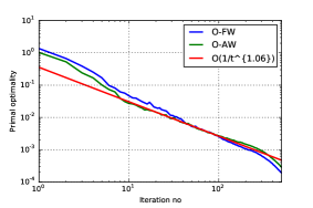
Figure 4: Online LASSO with single-pixel imaging data R64.mat. (Left) Convergence of the objective value. (Middle) Reconstructed image after $500$ iterations of O-FW; (Right) O-AW.

Figure 3 plots the primal optimality $h_{t}\mathrel{\mathop{:}}=f(\bm{\theta}_{t})-f(\bm{\theta}^{\star})$ with the round number $t$. The left figure corresponds to the scenario under H1 as $\bm{\theta}^{\star}$ belongs to the interior of ${\cal C}$. The simulation result corroborates with our analysis, which indicate a fast convergence rate of ${\cal O}(1/t)$. In the right figure, we observe that although H1 is not satisfied, the O-FW algorithm still maintains a convergence rate of $\sim{\cal O}(1/t)$, and O-AW is slightly outperforming O-FW. Examining the necessity of including H1 in achieving a fast convergence rate for O-FW will be left for future investigation. Lastly, the primal convergence rate of sPG is similar to O-FW. However, the per-iteration complexity of sPG is ${\cal O}(n\log n)$, while it is ${\cal O}(n)$ for the O-FW.

Realistic Data. We consider learning a sparse image $\bm{\theta}$ from the dataset R64.mat available from [DDT⁺08]. The dataset consists of $T=4319$ one-bit measurements of a greyscale image of ‘R’ with size $64\times 64$. The squared loss function is chosen such that $f_{t}(\bm{\theta})=(y_{t}-{\bm{a}}_{t}^{\top}\bm{\theta})^{2}$, where ${\bm{a}}_{t}\in\mathbb{R}^{n}$ is a binary measurement vector and $n=4096$ is the vectorized image. For the O-FW/O-AW algorithms, we have (i) used batch processing by drawing a batch of $B=5$ new observations and (ii) introduced an inner loop by repeating the O-FW/O-AW iterations, i.e., Line 4-5 of Algorithm 1 or Line 4-15 of Algorithm 2 for $50$ times within each iteration.

As the optimal solution $\bm{\theta}^{\star}$ is unavailable for this problem, Figure 4 compares the primal objective value $F_{T}(\bm{\theta}_{t})$ against the iteration number and the reconstructed image after $t_{f}=500$ iterations of the tested algorithms. The figure shows that the convergence rates of these algorithms all converge at a rate of $\sim{\cal O}(1/t)$.

References

• [ADX10] A. Agarwal, O. Dekel, and L. Xiao. Optimal algorithms for online convex optimization with multi-point bandit feedback. In COLT, 2010.
• [AZH16] Z. Allen-Zhu and E. Hazan. Variance reduction for faster non-convex optimization. In ICML, 2016.
• [BT09] A. Beck and M. Teboulle. A fast iterative shrinkage-thresholding algorithm for linear inverse problems. SIAM J. Imaging Sci., 2(1):183–202, 2009.
• [CL11] C.-C. Chang and C.-J. Lin. LIBSVM: A library for support vector machines. ACM Trans. on Intelligent Sys. and Tech., 2:27:1–27:27, 2011.
• [DDT+08] Marco Duarte, Mark Davenport, Dharmpal Takhar, Jason Laska, Ting Sun, Kevin Kelly, and Richard Baraniuk. Single-pixel imaging via compressive sampling. IEEE Signal Processing Magazine, 25(2):83–91, Mar 2008.
• [EBG11] S. Ertekin, L. Bottou, and C. Lee Giles. Nonconvex online support vector machines. IEEE Trans. on Pattern Analysis and Machine Intelligence, 33(2), Feb 2011.
• [EV76] Yu. M. Ermol’ev and P. I. Verchenko. A linearization method in limiting extremal problems. Cybernetics, 12(2):240–245, 1976.
• [FG13] Robert M. Freund and Paul Grigas. New analysis and results for the Frank-Wolfe method. CoRR, abs/1307.0873v2, 2013.
• [FW56] M. Frank and P. Wolfe. An algorithm for quadratic programming. Naval Res. Logis. Quart., 1956.
• [Gau05] Jean-Louis Verger Gaugry. Covering a ball with smaller equal balls in $n$. Discrete and Computational Geometry, 33:143–155, 2005.
• [GH15a] D. Garber and E. Hazan. Faster rates for the Frank-Wolfe method over strongly-convex sets. ICML, 2015.
• [GH15b] D. Garber and E. Hazan. A linearly convergent conditional gradient algorithm with applications to online and stochastic optimization. CoRR, abs/1301.4666, August 2015.
• [GHJY15] R. Ge, F. Huang, C. Jin, and Y. Yuan. Escaping from saddle points — online stochastic gradient for tensor decomposition. In COLT, 2015.
• [GL15] S. Ghosh and H. Lam. Computing worst-case input models in stochastic simulation. CoRR, abs/1507.05609, July 2015.
• [HJ94] R. A. Horn and C. R. Johnson. Topics in matrix analysis. Cambridge University Press, Cambridge, 1994. Corrected reprint of the 1991 original.
• [HK12] E. Hazan and S. Kale. Projection-free online learning. ICML, 2012.
• [HK15] F. M. Harper and J. A. Konstan. The movielens datasets: History and context. ACM TiiS, Jan 2015.
• [HL16] E. Hazan and H. Luo. Variance-reduced and projection-free stochastic optimization. In ICML, 2016.
• [HO14] C.-J. Hsieh and P. A. Olsen. Nuclear norm minimization via active subspace selection. In ICML, 2014.
• [Jag13] M. Jaggi. Revisiting Frank-Wolfe: Projection-free sparse convex optimization. ICML, 2013.
• [JLMZ16] Bo Jiang, Tianyi Lin, Shiqian Ma, and Shuzhong Zhang. Structured nonconvex and nonsmooth optimization: Algorithms and iteration complexity analysis. CoRR, May 2016.
• [JN12a] A. B. Juditsky and A. S. Nemirovski. First-Order Methods for Nonsmooth Convex Large-Scale Optimization, I: General Purpose Methods. 2012.
• [JN12b] A. B. Juditsky and A. S. Nemirovski. First-Order Methods for Nonsmooth Convex Large-Scale Optimization, II: Utilizing Problem’s Structure. 2012.
• [Klo14] O. Klopp. Noisy low-rank matrix completion with general sampling distribution. Bernoulli, 2(1):282–303, 02 2014.
• [Kol13] V. Koltchinskii. A remark on low rank matrix recovery and noncommutative Bernstein type inequalities, volume Volume 9 of Collections, pages 213–226. Institute of Mathematical Statistics, 2013.
• [LJ16] S. Lacoste-Julien. Convergence rate of frank-wolfe for non-convex objectives. CoRR, July 2016.
• [LJJ13] S. Lacoste-Julien and M. Jaggi. An affine invariant linear convergence analysis for Frank-Wolfe algorithms. NIPS, 2013.
• [LJJ15] S. Lacoste-Julien and M. Jaggi. On the global linear convergence of Frank-Wolfe optimization variants. In NIPS. 2015.
• [LZ14] G. Lan and Y. Zhou. Conditional gradient sliding for convex optimization. Tech. Report, 2014.
• [NJLS09] A. Nemirovski, A. Juditsky, G. Lan, and A. Shapiro. Robust stochastic approximation approach to stochastic programming. SIAM J. Optim., 2009.
• [RR11] M. Raginsky and A. Rakhlin. Information-based complexity, feedback and dynamics in convex programming. IEEE Trans. Inf. Theory, 57(10):7036–7056, October 2011.
• [RVV14] L. Rosasco, S. Villa, and Bang Cong Vu. Convergence of Stochastic Proximal Gradient Algorithm. CoRR, abs/1403.5074v3, 2014.
• [SSSS11] S. Shalev-Shwartz, Ohad Shamir, and Karthik Sidharan. Learning kernel-based halfspaces with the 0-1 loss. SIAM J. Comput., 40(6):1623–1646, 2011.
• [SSSSS09] S. Shalev-Shwartz, O. Shamir, N. Srebro, and K. Sridharan. Stochastic convex optimization. COLT, 2009.
• [Wol70] P. Wolfe. Convergence theory in nonlinear programming. Integer and Nonlinear Program., 1970.
• [YZS14] Yaoliang Yu, Xinhua Zhang, and Dale Schuurmans. Generalized conditional gradient for sparse estimation. CoRR, Oct 2014.