Clustered Low-Rank Tensor Format: Introduction and Application to Fast Construction of Hartree-Fock Exchange

Abstract

Clustered Low Rank (CLR) framework for block-sparse and block-low-rank tensor representation and computation is described. The CLR framework depends on 2 parameters that control precision: one controlling the CLR block rank truncation and another that controls screening of small contributions in arithmetic operations on CLR tensors. As these parameters approach zero CLR representation and arithmetic become exact. There are no other ad-hoc heuristics, such as domains. Use of the CLR format for the order-2 and order-3 tensors that appear in the context of density fitting (DF) evaluation of the Hartree-Fock (exact) exchange significantly reduced the storage and computational complexities below their standard $\mathcal{O}\left(N^{3}\right)$ and $\mathcal{O}\left(N^{4}\right)$ figures. Even for relatively small systems and realistic basis sets CLR-based DF HF becomes more efficient than the standard DF approach, and significantly more efficient than the conventional non-DF HF, while negligibly affecting molecular energies and properties.

I Introduction

Despite the exponential complexity of many-body quantum mechanics – a manifestation of “the curse of dimensionality” – many important classes of problems, such as electronic structure in chemistry and materials science, have robust polynomial solutions that become exact for practical purposes.Tajti:2004hwa ; Bomble:2006dv ; Harding:2008cn ; Shiozaki:2009ix ; Booth:2013er ; Yang:2014jc However, such solutions are limited by the high-order polynomial complexity of data and operations. For example, the straightforward implementation of CCSDScuseria:1988dn – the coupled-clusterBartlett:1981hg model with 1-body and 2-body correlations – has $\mathcal{O}\left(N^{6}\right)$ and $\mathcal{O}\left(N^{4}\right)$ operation and data complexities, respectively. This is significantly more expensive than the corresponding $\mathcal{O}\left(N^{4}\right)$ and $\mathcal{O}\left(N^{2}\right)$ complexities of hybrid Kohn-Sham density functional theory (KS DFT) that dominates chemistry applications. Thankfully it is possible to improve on these figures.

Fast numerical algorithms trade off precision and/or small-$N$ cost for improved asymptotic scaling. A classic example is Strassen’s algorithm for matrix multiplicationStrassen:1969uw that has higher operation count than the naïve algorithm for small matrices but is faster for large matrices, namely $\mathcal{O}\left(N^{\log_{2}7}\right)$ vs. $\mathcal{O}\left(N^{3}\right)$. Operation count of Strassen-based implementation of CCSD is therefore $\mathcal{O}\left(N^{2\log_{2}7}\right)\approx\mathcal{O}\left(N^{5.6}\right)$. Another notable fast algorithm of particular importance to the field of electronic structure is Fast Multipole Method (FMM)Greengard:1987gi ; White:1994ip applies an integral (e.g. Coulomb) operator in $\mathcal{O}\left(N\right)$ operations, instead of $\mathcal{O}\left(N^{2}\right)$, for any finite precision $\epsilon$.

In molecular electronic structure fast algorithms are traditionally predicated on taking advantage of the sparse structure of the operators and states. Such structure in most cases takes form of the element or block sparsity. For example, the one-electron density matrix is conjecturedKohn:1996hn ; Li:1993jra ; Millam:1997cla to decay exponentially in insulators when expressed in localized basis (AO or Wannier); this is the foundation of fast density matrix minimization in one-particle theories and also leads to the exponential decay of the “exact” (Hartree-Fock) exchange operator appearing in hybrid DFT and many-body methods. Linear scaling methods based on such strategy have been demostrated by multiple groups.Ochsenfeld:2007vwa ; Niklasson:2003hha ; Shao:2003hya ; Challacombe:1999bpa ; Palser:1998uk ; Millam:1997cla While the element-sparsity-based strategy is appropriate for LCAO in small basis sets and low-dimensional systems, the sparsity of density matrix in three-dimensional systems is remarkably low,Rudberg:2008cba ; Rudberg:2011km ; VandeVondele:2012ho especially when expressed in realistic (triple- and higher-$\zeta$) basis sets necessary for many-body methods and even hybrid DFT; e.g., the density matrix of a 32000-molecule water cluster is only 83% sparse (!) even when expressed in a double-$\zeta$ basis.VandeVondele:2012ho Similar conclusions can be drawn from the early attempts to develop practical many-body methods solely by using sparsity of correlation operators in AO basis.Scuseria:1999bp It is clear that the element sparsity alone is hardly sufficient for practical fast electronic structure. Another structure used in fast electronic structure methods is rank sparsity. For example, the Coulomb operator, $\hat{V}f(x)\equiv\int\mathrm{d}x\,f(x^{\prime})/|x-x^{\prime}|$, has a dense matrix representation due to slow decay of the integral kernel, but the rank of off-diagonal blocks when expressed in localized basis is low due to the smoothness of the kernel; of course, this is the basis of FMM.Greengard:1987gi The key lesson here is that while globally the Coulomb operators has no non-trivial rank-sparsity, ranks of off-diagonal blocks are low. Remarkably, similar local rank-sparsity is exploitable in other contexts. For example, blocks of many-body wave functions have low rank when expressed in localized basis; such rank-sparsity is the foundation of fast many-body methods based on local pair-natural orbitals (PNO)Neese:2009kpa recently demonstrated in linear-scaling form.Riplinger:2013jk ; Pinski:2015ii

In this work we propose a practical approach to recovering element and rank sparsities (termed here data sparsity) by using a general tensor format framework called Clustered Low-Rank (CLR, pronounced as “CLeaR”). Some existing approaches, such as PNO-based many-body methods, can be viewed as a specialized application of CLR. However, we demonstrate in the following discussion that CLR has powerful applications beyond this particular context.

The theoretical underpinnings of CLR come from the study of semi-separable Vandebril:2005fi ; Chandrasekaran:2005kv , hierarchically semi-separableXia:2010kx , and $\mathcal{H}$- matrices.Hackbusch:1999jh ; Hackbusch:2000fx ; Grasedyck:2003ij Other researchers have mentioned this type of approximation, with regards to electronic structure, before, namely Bock:2013ixa, where the idea was only mentioned in passing and very recently benner2015reduced, where a rank structured approach was used to reduce computational complexity in the solution to the Bethe-Salpeter equation. These can be viewed as algebraic generalizations of the rank-sparse structure arising in integral boundary problems, studied first by RokhlinRokhlin:1985ig and HackbuschHackbusch:1989tn . Later Tyrtyshnikov realized that this type of approximation could be generalized to matrices arising in integral equations via a method he calls the mosaic-skeleton approximation (MSA) where the integral kernel satisfies some necessary conditions.Tyrtyshnikov:1996fd He expands on this idea suggesting that for matrices that fit the necessary conditions there exists a non-overlapping blocking called a mosaic in which many of the blocks have reduced rank.tyrtyshnikov1997bookchap ; Goreinov:1997hh Soon after Hackbusch premiered the $\mathcal{H}$-matrix concept, where $\mathcal{H}$ stands for hierarchical, in which he formalizes his integral approximation methods into a general matrix framework. The main difference between Tyrtyshnikov and Hackbusch’s generalizations are that $\mathcal{H}$-matrices have a hierarchical block structure while the MSA approach does not. In this regard CLR can be viewed as a refinement of MSA for general tensor data; the lack of hierarchy is deemed important for compatibility with standard algorithms for matrix and tensor algebra in high-performance computing that embed blocked tensors onto a regular cartesian grid of processors.

The rest of the paper is organized as follows: in section II we will discuss the details of CLR, in section III we discuss an application of CLR to density fitting approximation in the context of the Hartree-Fock (exact) exchange evaluation, and in section IV we discuss our findings as well as future directions for CLR.

II Clustered Low Rank Approach

CLR, in a general sense, may be thought of as a tensor representation framework, which divides a tensor into sub-blocks (tiles) that are stored in either low-rank or full-rank (dense) form. For example, consider a real-valued, order-$k$ tensor with dimension sizes $\{n_{1}\dots n_{k}\}$:

$${\bf T}:\mathbf{x}\to\mathbb{R},\quad\forall\mathbf{x}\equiv\{x_{1}\dots x_{k}\},x_{i}\in[1,n_{i}]\,\forall i=1,k,$$ (1)

with tensor elements denoted as $T_{\mathbf{x}}\equiv T_{x_{1}\dots x_{k}}={\bf T}(\mathbf{x})$. CLR representation of T is defined as follows:

1. Each dimension $i$ is tiled into $\nu_{i}\geq 2$ blocks (tiles) of sizes $\{\beta_{1}\dots\beta_{\nu_{i}}\}$:

   $$\tau_{i}: \{1\dots n_{i}\}\to\{\mathcal{X}^{(i)}_{\xi}\},\xi\in[1,\nu_{i}],\quad\mathrm{where}$$ (2)

   $$\mathcal{X}^{(i)}_{\xi} \equiv\{x^{(\xi)}_{1}\dots x^{(\xi)}_{\beta_{j}}\}$$ (3)

   Tiling of a tensor domain is then obtained as a tensor product of dimension tilings, $\tau\equiv\tau_{1}\otimes\dots\tau_{k}$ so that each block index $\boldsymbol{\xi}\equiv\{\xi_{1}\dots\xi_{k}\}$ defines block of element indices $\mathcal{X}_{\boldsymbol{\xi}}\equiv\mathcal{X}^{(1)}_{\xi_{1}}\otimes\dots\mathcal{X}^{(k)}_{\xi_{k}}$. The corresponding tensor tile,

   $${\bf T}_{\boldsymbol{\xi}}\equiv{\bf T}_{\mathcal{X}^{(1)}_{\xi_{1}}\dots\mathcal{X}^{(k)}_{\xi_{k}}}=\{T_{x_{1}\dots x_{k}}:x_{j}\in\mathcal{X}^{(j)}_{\xi_{j}},\forall j\in[1,k]\},$$ (4)

   is also an order-$k$ tensor.

2. The (optional) shape predicate $z(\boldsymbol{\xi})$ defines whether block $\boldsymbol{\xi}$ is set to zero.

3. Each tensor block ${\bf T}_{\boldsymbol{\xi}}$ is data-compressed using a low-rank tensor decomposition.

It is evident from the above description that CLR is similar to $\mathcal{H}$-matrices and MSA with respect to the structure of the matrix representations. However, the choice of tiling, shape, and low-rank decomposition schemes as well as the specific application chemical knowledge differentiates these methods. In the following sections, we will specialize CLR for a particular set of matrices. But first we should discuss the design elements of CLR framework.

• Basis elements are reordered into spatially localized clusters that form the non-overlapping tile partitions of CLR matrices (see Section II.1 for details). This tiling structure is essential for both improved data locality in the context of parallel computing,Weber:2015kr and data compression in low-rank tiles.

• The shape defines block-sparse structure of CLR matrices, which may be based on the magnitude of tile norms (or norm estimates), an imposed sparsity model, or a combination of these methods. Many useful electronic structure methods impose block sparsity, e.g. the use of AO domains in local density fitting and local correlation. Although low-rank decomposition of blocks naturally reveals block sparsity, the preemptive introduction of block sparsity can lead to additional computational savings.

• Low-rank decomposition of tensor tiles is used to reduce the total storage requirements for high-order (greater than order-two) tensors. The choice of decomposition methods is problem specific due to the fact that, with the exception of matrices, tensor rank is not uniquely defined, nor is there an optimal decomposition for tensors. Even for matrices, SVD is often not the optimal choice due to its high computational cost.

• Another factor in the choice of decomposition is the suitability an algorithm for use in algebraic operations, where frequent recompressions will often be necessary. For example, given a matrix, SVD will always provide the most compact low-rank representation for a given accuracy, but it may be beneficial to sacrifice storage or accuracy in certain cases for computational efficiency.

To demonstrate the usefulness of the CLR framework in practical applications, we applied it to fast construction of the Hartree-Fock (exact) exchange using density fitting (DF) as our first example. DF (also known as resolution of the identity) technology allows us to reduce the computational cost of the Fock operator construction by decreasing the prefactor, especially when triple- or higher-$\zeta$ basis sets are used. However, for large molecules DF HF performs poorly, relative to conventional HF methods, due to the $\mathcal{O}\left(N^{3}\right)$ storage and $\mathcal{O}\left(N^{4}\right)$ operation complexities. Meanwhile even the naïve implementation of conventional HF methods only require quadratic storage, and $\mathcal{O}\left(N\right)$ approaches to exchange build in LCAO representation are well-known.Schwegler:1996hh ; Burant:1996cf ; Ochsenfeld:1998p1663 ; Neese:2009ca The goal of our work is therefore to develop a CLR-based DF HF method with reduced storage and computation complexities.

The DF HF method deals with at most order-3 tensors, e.g. the so-called three-center two-electron Coulomb integral:

$$(\kappa|\mu\nu) \equiv\iint\phi_{\kappa}(\mathbf{r}_{1})\frac{1}{r_{12}}\phi^{*}_{\mu}(\mathbf{r}_{2})\phi_{\nu}(\mathbf{r}_{2})\,d\mathbf{r}_{1}d\mathbf{r}_{2}\text{.}$$ (5)

An effective low-rank representation of such tensors can be obtained by treating its blocks as matrices, where $\mu$ and $\nu$ forms a single index space. Hence, we describe in detail use of CLR for compressed representation and operation of matrices and matrix-like tensors.

II.1 Basis Clustering

To tile AOs as well as occupied molecular orbitals (MO) in this work we utilized the k-means clustering algorithmLloyd:1982do ; Jain:2010cu with a Euclidean distance metric. Given a set of Cartesian coordinates $\{\mathbf{r}_{1},\mathbf{r}_{2},\dots,\mathbf{r}_{m}\}$ in $\mathbb{R}^{n}$ (atomic coordinates when clustering atoms/AOs, or the expectation values of $\hat{\mathbf{r}}$ when clustering MOs) and the target number of clusters $m$, k-means seeks clusters that minimize

$$\sum_{i=1}^{m}\sum_{\mathbf{r}\in\mathcal{X}_{i}}||\mathbf{r}-\mathbf{R}_{i}||^{2}\text{,}$$ (6)

where $\mathbf{R}_{i}$ is the center of mass of cluster $\mathcal{X}_{i}$ for clustering atoms or the centroid when clustering MOs. To determine the clusters, we use the k-means++ algorithmarthur2007k to seed starting points, and then proceed to perform the standard k-means; the only exception is that hydrogen atoms are always forced into the same clusters as their nearest non-hydrogen atom. We stop when all centers of mass reach a (local) minima, or after 100 iterations. The procedure is repeated 10 times with random starting seeds. From these 10 clusterings we use the one that has the lowest value for the objective function, (6).

II.2 Block Sparsity in CLR Tensors

Tensors like that in equation (5) become increasingly sparse for large molecules when expressed in a localized basis. Thus, it is mandatory to estimate norms of the blocks to avoid evaluation of vanishing blocks. For the Coulomb 3-index tensor (5) in an AO basis, this is readily done by using AO shell-wise integral estimators, e.g. ref Hollman:2015ca, . An extension to atom and multi-atom blocks is straightforward. The block-norm estimates define the sparsity of the tensors (see section II.4 for details). For simplicity and clarity in this work, we did not preemptively skip computation of any integrals. This will be addressed in future work.

II.3 Low-Rank Block Representation and Arithmetic

Each block of a CLR matrix is potentially represented in a low-rank form. Before discussing multiplication and addition of CLR matrices, we must first consider the block-level operations in low-rank representation.

II.3.1 Low-Rank Matrix Approximation

Matrix $\mathbf{A}_{r}\in\mathbb{R}^{n\times m}$ has rank $r\leq\min{(n,m)}$ if it can be represented exactly as a sum of outer products of no fewer than $r$ linearly independent vectors

$$\mathbf{A}_{r} =\sum_{i=1}^{r}\mathbf{s}_{i}^{\mathbf{A}}\left(\mathbf{t}_{i}^{\mathbf{A}}\right)^{\dagger}\text{,}$$ (7)

$$\equiv\mathbf{S}^{\mathbf{A}}\left(\mathbf{T}^{\mathbf{A}}\right)^{\dagger}\text{,}$$ (8)

where $\mathbf{S}^{\mathbf{A}}\equiv\{\mathbf{s}_{1}^{\mathbf{A}},\mathbf{s}_{2}^{\mathbf{A}},\dots\mathbf{s}_{r}^{\mathbf{A}}\}$ and $\mathbf{T}^{\mathbf{A}}\equiv\{\mathbf{t}_{1}^{\mathbf{A}},\mathbf{t}_{2}^{\mathbf{A}},\dots\mathbf{t}_{r}^{\mathbf{A}}\}$. We seek to approximate a full-rank matrix $\mathbf{A}$ with a rank-$r$ matrix $\mathbf{A}_{r}$ which both minimizes

$$||\mathbf{A}-\mathbf{A}_{r}||_{F}\leq\epsilon_{\mathrm{lr}}$$ (9)

and allows for efficient arithmetic in decomposed form. Therefore, we approximate matrices using column pivoted (rank-revealing) QR decomposition (RRQR). RRQR is faster than SVD and approximates the SVD (optimal) ranks well.Chan:1987tq ; QuintanaOrti:2006df ; Bischof:1998hc The RRQR decomposition decomposes a matrix $\mathbf{A}$ as:

$$\mathbf{AP} =\mathbf{QR}\equiv\mathbf{Q}\begin{pmatrix}R_{11}&R_{12}\\ 0&R_{22}\end{pmatrix}\text{.}$$ (10)

The singular values of the matrix may be estimated, by computing $||\mathbf{R}_{22}||_{F}$, according to:

$$\sigma_{m-r+1}\leq||\mathbf{R}^{r}_{22}||_{2}\leq||\mathbf{R}^{r}_{22}||_{F}\text{,}$$ (11)

for $\mathbf{R}\in\mathbb{R}^{m\times m}$. To estimate the rank of $\mathbf{A}$ we compute $\mathbf{R}$ (using the DGEQP3 LAPACK function) and walk up the lower triangle from element $R_{mm}$ to compute norms $||\mathbf{R}^{r}_{22}||_{F}$, stopping once the norm is larger than our threshold. While this method will potentially lead to larger ranks that using the SVD decomposition, in practice RRQR does a adequate job of revealing rank while having a reduced prefactor.

Another consideration is that we consider a matrix low rank if for threshold $\epsilon_{\mathrm{lr}}$ matrix $\mathbf{A}\in\mathbb{R}^{m\times n}$ has rank $r_{A}<\text{min}\left(m,n\right)$, but just because a matrix is low rank does not mean that there are computational or storage savings. Given a square matrix in $\mathbb{R}^{m\times m}$ it is necessary that $r<\frac{m}{2}$ for there to be storage savings from storing $\mathbf{S}$ and $\mathbf{T}$ for the matrix. Thus any time the storage of $\mathbf{S}+\mathbf{T}$ is greater than the storage of $\mathbf{C}$ we convert the tensor to full rank form.

II.3.2 Multiplication of Low-Rank Matrices

Clearly, $\mathbf{C}=\mathbf{A}\mathbf{B}$ can be directly computed in low-rank form $\mathbf{C}=\mathbf{S}^{\mathbf{C}}\left(\mathbf{T}^{\mathbf{C}}\right)^{\dagger}$ using low-rank representations of $\mathbf{A}$ and $\mathbf{B}$ with rank $\min(\operatorname{rank}(\mathbf{A}),\operatorname{rank}(\mathbf{B}))$:

$$\mathbf{S}^{\mathbf{C}}\left(\mathbf{T}^{\mathbf{C}}\right)^{\dagger}= \mathbf{S}^{\mathbf{A}}\left(\mathbf{T}^{\mathbf{A}}\right)^{\dagger}\mathbf{S}^{\mathbf{B}}\left(\mathbf{T}^{\mathbf{B}}\right)^{\dagger}$$ (12)

$$= \begin{cases}\mathbf{S}^{\mathbf{A}}\left(\left(\left(\mathbf{T}^{\mathbf{A}}\right)^{\dagger}\mathbf{S}^{\mathbf{B}}\right)\left(\mathbf{T}^{\mathbf{B}}\right)^{\dagger}\right)&r_{A}<r_{B}\\ \left(\mathbf{S}^{\mathbf{A}}\left(\left(\mathbf{T}^{\mathbf{A}}\right)^{\dagger}\mathbf{S}^{\mathbf{B}}\right)\right)\left(\mathbf{T}^{\mathbf{B}}\right)^{\dagger}&r_{A}\geq r_{B}\end{cases},$$ (13)

in which the order of evaluation and hence the definitions of $\mathbf{S}^{\mathbf{C}}$ and $\mathbf{T}^{\mathbf{C}}$ are specified by the parentheses. Note that the multiplication never increases matrix rank.

The special cases where either $\mathbf{A}$ or $\mathbf{B}$ is full rank are also completely straightforward.

II.3.3 Addition of Low-Rank Matrices

Unlike the multiplication, addition of low-rank matrices may increase rank as can be immediately seen:

$$\mathbf{C}= \mathbf{S}^{\mathbf{A}}\left(\mathbf{T}^{\mathbf{A}}\right)^{\dagger}+\mathbf{S}^{\mathbf{B}}\left(\mathbf{T}^{\mathbf{B}}\right)^{\dagger}$$

$$= \mathbf{S}^{\mathbf{A+B}}\left(\mathbf{T}^{\mathbf{A+B}}\right)^{\dagger}$$ (14)

where $\mathbf{S}^{\mathbf{A+B}}=\{\mathbf{S}^{\mathbf{A}},\mathbf{S}^{\mathbf{B}}\}$ and $\mathbf{T}^{\mathbf{A+B}}=\{\mathbf{T}^{\mathbf{A}},\mathbf{T}^{\mathbf{B}}\}$. The maximum rank of $\mathbf{C}$ in (II.3.3) is the sum of the ranks of $\mathbf{A}$ and $\mathbf{B}$ if columns of $\mathbf{S}^{\mathbf{A+B}}$ and/or $\mathbf{T}^{\mathbf{A+B}}$ are linearly independent. Of course it is often the case that the ranks of these matrices can be reduced further with controlled error. We can reduce the ranks of $\mathbf{S}^{\mathbf{A+B}}$ and $\mathbf{T}^{\mathbf{A+B}}$ as follows. Starting with QR decompositions of these matrices,

$$\mathbf{S}^{\mathbf{A+B}} =\mathbf{Q}^{\mathbf{S}}\mathbf{R}^{\mathbf{S}}$$ (15)

$$\mathbf{T}^{\mathbf{A+B}} =\mathbf{Q}^{\mathbf{T}}\mathbf{R}^{\mathbf{T}}\text{,}$$ (16)

(II.3.3) is rewritten

$$\mathbf{C} =\mathbf{Q}^{\mathbf{S}}\mathbf{R}^{\mathbf{S}}\left(\mathbf{R}^{\mathbf{T}}\right)^{\dagger}\left(\mathbf{Q}^{\mathbf{T}}\right)^{\dagger}\text{,}$$ (17)

Intermediate $\mathbf{M}\equiv\mathbf{R}^{\mathbf{S}}\left(\mathbf{R}^{\mathbf{T}}\right)^{\dagger}$ is then RRQR decomposed resulting in reduced rank $r\leq\operatorname{rank}\mathbf{A}+\operatorname{rank}\mathbf{B}$.

$$\mathbf{M}=\widetilde{\mathbf{Q}}\widetilde{\mathbf{R}}\overset{\epsilon_{\mathrm{lr}}}{\approx}\widetilde{\mathbf{Q}}_{r}\widetilde{\mathbf{R}}_{r}$$ (18)

where for $\widetilde{\mathbf{Q}}$ and $\widetilde{\mathbf{R}}$ the tilde signifies RRQR as oppose to traditional QR.

The final result for the low-rank form of $\mathbf{C}$ is

$$\mathbf{C} =\left(\mathbf{Q}^{\mathbf{S}}\widetilde{\mathbf{Q}}_{r}\right)\left(\widetilde{\mathbf{R}}_{r}\left(\mathbf{Q}^{\mathbf{T}}\right)^{\dagger}\right)\equiv\mathbf{S}^{C}\left(\mathbf{T}^{C}\right)^{\dagger}\text{,}$$ (19)

where

$$\mathbf{S}^{C} =\mathbf{Q}^{\mathbf{S}}\widetilde{\mathbf{Q}}_{r}$$ (20)

$$\left(\mathbf{T}^{C}\right)^{\dagger} =\widetilde{\mathbf{R}}_{r}\left(\mathbf{Q}^{\mathbf{T}}\right)^{\dagger}.$$ (21)

if after compression $\operatorname{rank}\mathbf{C}\geq\frac{\rm fullrank}{2}$ then $\mathbf{C}$ is converted to its full rank representation since no space savings is available.

When performing addition if exactly one of $\mathbf{A}$ or $\mathbf{B}$ is in the full rank representation, we perform the addition using a generalized matrix-matrix multiplication (GEMM). For example if $\mathbf{A}$ is low rank and $\mathbf{B}$ is full rank the addition proceed as follows:

$$\mathbf{C}=\mathbf{S}^{\mathbf{A}}\left(\mathbf{T}^{\mathbf{A}}\right)^{\dagger}+\mathbf{B}\text{,}$$ (22)

where $\mathbf{C}$ is in its full rank representation. The addition in equation (22) is able to take advantage of optimized linear algebra libraries and avoid the storage overhead of constructing a temporary of $\mathbf{A}$.

II.4 Block-Sparse Arithmetic with CLR Tensors

An arithmetic operation on matrices/tensors composed of CLR-format blocks can be performed as a standard operations on dense matrices/tensors with standard block operations replaced by their CLR specializations. For the sake of computational efficiency, however, it is necessary to screen arithmetic expressions involving CLR-format blocks to avoid laboriously computing blocks that have small norm and hence low rank. Therefore we represent CLR matrices/tensors as their block-sparse counterparts, in which only some blocks are deemed to have non-zero norms; the surviving blocks are represented using CLR format. This allows us to exploit both block-sparsity and block-rank-sparsities. In the limit $\epsilon_{\mathrm{lr}}\to 0$, CLR matrices/tensors become their ordinary block-sparse counterparts. Here we describe how we utilize block-sparse structure of CLR tensors in arithmetic operations.

Block ${\bf A}_{\boldsymbol{\xi}}$ of CLR tensor ${\bf A}$ that is the result of an arithmetic operation is nonzero (hence, it will be computed) if its Frobenius norm satisfies

$$\|{\bf A}_{\boldsymbol{\xi}}\|_{\rm F}\geq\epsilon_{\rm sp}\operatorname{area}{{\bf A}_{\boldsymbol{\xi}}}$$ (23)

where $\epsilon_{\rm sp}$ is a non-negative threshold, and $\operatorname{area}{\bf A}_{\boldsymbol{\xi}}$ is the block area, i.e. the number of elements in the block. Because the area of each block within a tensor may vary significantly, the sparsity threshold is scaled by the block area to provide a consistent sparsity criteria with a single parameter.

The sub-multiplicative property of Frobenius norm is utilized to estimate the norm in addition and contraction operations, e.g. for addition

$$\|{\bf A}_{\boldsymbol{\xi}}+{\bf B}_{\boldsymbol{\xi}}\|_{\rm F}\leq\|{\bf A}_{\boldsymbol{\xi}}\|_{\rm F}+\|{\bf B}_{\boldsymbol{\xi}}\|_{\rm F}$$ (24)

the upper bound provided by the RHS is used to estimate whether computing the block is warranted according to (23). Similarly, the norm of a contraction of two tensor blocks is bounded as

$$\begin{split}\|{\bf A}_{\xi_{i}\dots\xi_{k}\dots}&{\bf B}_{\xi_{k}\dots\xi_{j}\dots}\|_{\rm F}\\ \leq&\|{\bf A}_{\xi_{i}\dots\xi_{l}\dots}\|_{\rm F}\|{\bf B}_{\xi_{l}\dots\xi_{j}\dots}\|_{\rm F}\end{split},$$ (25)

where $\xi_{i}\dots$ and $\xi_{j}\dots$ are the outer block indices of the left- and right-hand tensors, respectively, and $\xi_{k}\dots$ is the set of block summation indices. Eqs. (24), and (25) are combined to estimate the norm of the result blocks in a contraction operations:

$$\begin{split}\|{\bf C}_{\xi_{i}\dots\xi_{j}\dots}\|\leq\sum_{k}\|{\bf A}_{\xi_{i}\dots\xi_{k}\dots}\|_{\rm F}\|{\bf B}_{\xi_{k}\dots\xi_{j}\dots}\|_{\rm F}\end{split}$$ (26)

where ${\bf C}_{i\dots j\dots}$ is equal to $\sum_{k\dots}{\bf A}_{i\dots k\dots}{\bf B}_{k\dots j\dots}$. Note that we do not screen individual contributions to the result blocks, i.e. all contributions are computed if the estimated result block norm satisfies Eq. (23).

Additionally, we avoid explicit computation of norms of low-rank blocks by using the multiplicative property of Frobenius norm:

$$\|{\bf A}_{\boldsymbol{\xi}}\|\approx\|{\bf S}^{\bf A}_{\boldsymbol{\xi}}({\bf T}^{\bf A}_{\boldsymbol{\xi}})^{\dagger}\|_{\rm F}\leq\|{\bf S}^{\bf A}_{\boldsymbol{\xi}}\|_{\rm F}\|{\bf T}^{\bf A}_{\boldsymbol{\xi}}\|_{\rm F}\text{.}$$ (27)

It is clear that computing norm estimates in complex expressions using upper bounds can quickly lead to poor norm estimates. Therefore, it is sometimes necessary to recompute the block norms and/or truncate zero blocks that are the result of computation. Similarly, after a CLR tensor contraction or addition operation it is possible that the rank of certain blocks are larger than necessary. Therefore in this work we sometimes recompute block norms and recompression after tensor contractions to minimize the ranks and reduce the storage.

III Application: CLR-based Density Fitting in Hartree-Fock Method

III.1 Density Fitting and Hartree-Fock Method

Density fitting (also known as the resolution-of-the-identity)Whitten:1973ju ; Baerends:1973p41 ; Feyereisen:1993di ; Vahtras:1993wy ; Dunlap:2000ii in the context of electronic structure involves fitting the electron density or more often any product of (one-electron) functions as a linear combination of basis functions from a fixed (auxiliary) basis set to minimize some functional. This allows us to compute standard 4-center 2-electron integrals in terms of 2- and 3-center integrals:

$$\left(\mu\nu|\rho\sigma\right) \approx\sum_{QP}E_{Q,\mu\nu}\left(\mathbf{V}^{-1}\right)_{Q,P}E_{P,\rho\sigma}$$ (28)

$$=\sum_{X}B_{X,\mu\nu}B_{X,\rho\sigma}\text{,}$$ (29)

$$B_{X,\mu\nu} \equiv\sum_{Q}E_{Q,\mu\nu}\left(\mathbf{V}^{-1/2}\right)_{Q,X}$$ (30)

where $E_{Q,\mu\nu}\equiv\left(Q|\mu\nu\right)$ (defined in Eq. (5)) and $V_{P,Q}\equiv(P|Q)$ are the three- and two-center Coulomb integrals. In practice, instead of $\mathbf{V}^{-1/2}$ we use the inverse of Cholesky decomposition of $\mathbf{V}$; this is cheaper than computing the square root inverse and incidentally leads to better CLR compression in $\mathbf{B}$.

There are many different strategies for using density fitting in Hartree-Fock. Here we pick a basic approach that instead of the density matrix uses occupied MOs (or any other factorization of the density)Kendall:1997kh (additional improvements such as the use of local density fittingGallant:1996ua ; Snijders:1998jr ; Watson:2003eo ; Merlot:2013ep ; Hollman:2014gc and computing only the occupied section of exchange matrixManzer:2015de can be also incorporated in our CLR-based scheme):

1. Compute and store $\mathbf{B}$ from equation 29.

2. Form $\mathbf{J}$, the coulomb contribution to the Fock matrix in $\mathcal{O}\left(n^{3}\right)$ steps via

   $$J_{\mu\nu} =\sum_{X}B_{X,\mu\nu}\sum_{\rho\sigma}B_{X,\rho\sigma}D_{\rho\sigma}$$ (31)

   where $\mathbf{D}$ is the AO density matrix.

3. Compute an intermediate tensor $\mathbf{W}$ with one index transformed from the AO to MO space as follows

   $$W_{X,\mu i} =\sum_{\sigma}B_{X,\mu\sigma}C_{\sigma i}$$ (32)

   where the column vectors of $\mathbf{C}$ are the occupied molecular orbitals.

4. Form the exchange contribution to the Fock matrix

   $$K_{\mu\nu} =\sum_{Xi}W_{X,\mu i}W_{X,\nu i}\text{.}$$ (33)

The two most expensive steps in forming the Fock matrix this way are formation of $\mathbf{W}$ and $\mathbf{K}$, which both require approximately $\mathcal{N}n^{2}o$ steps where $\mathcal{N}$ is the size of the auxiliary basis and $o$ is the number of occupied orbitals in the system.

Although the use of density fitting in Hartree-Fock method has the same formal complexity as conventional Fock operator construction, namely $\mathcal{O}\left(N^{4}\right)$ due to the exchange computation, there is significant reduction in prefactor for large orbital basis (triple-$\zeta$ and larger) due to avoiding the relatively expensive and repeated (once-per-iteration) computation of 4-center integrals. These advantages are exacerbated by the poor suitability of highly-irregular integral kernels to modern wide-SIMD architectures; in contrast, the dense matrix arithmetic of Eq. (29) can perform close to peak on most modern architectures provided the dimension sizes are large.

Despite the cost advantages of DF, its cubic storage requirements and quartic cost prohibit direct application to large systems. Local density fitting reduces the storage and computational complexity of density fitting by expanding localized products in terms of auxiliary basis functions that are “nearby” in some sense (geometric or otherwise) Local DF approximations can be difficult to make robust, thus in this work we decided to investigate whether a black-box reduced-scaling density fitting methodology can be obtained by the use of CLR format in the context of the Hartree-Fock method.

III.2 CLR-based Density Fitting Hartree-Fock

Implementation of CLR-based DF HF method used the 4-step formulation listed above. All dimensions were blocked naturally except for the index corresponding to the auxiliary basis, which uses larger blocks for performance reasons. Natural blocking consists of one block per water for water clusters and one block per CH₂ or CH₃ for n-alkanes. For the auxiliary basis we set the number of clusters to be half the number of natural clusters and use our k-means algorithm described previously in II.1 to determine clusters. Blocks of all three-index tensors were represented as low-rank matrices by merging the orbital indices together; the details of tensor arithmetic in this representation were described in Section II.

To simplify the initial implementation we use a cubically-scaling eigensolve-based solver for the Hartree-Fock; we will switch to a $\mathcal{O}\left(N\right)$ density minimization in the future. Instead of using occupied eigenorbitals directly we utilized orbitals obtained by pivoted Cholesky decomposition of the density matrix (LAPACK function DPSTRF), which are known to be more localized,Aquilante:2006dq to increase the data sparsity of tensor $\mathbf{W}$.

The CLR DF HF method was implemented with the help of the open-source TiledArray parallel tensor framework.TiledArray

III.3 Results

To gauge the robustness of CLR DF HF we computed energies and electric dipole moments of quasi-1-d (n-alkanes with linear geometry) and 3-d (water clusters) systems. Cartesian geometries for n-alkanes were generated using Open Babel.OLBoyle:2011wz Cartesian coordinates for the water clusters were taken from ErgoSCF’s public repositoryErgoWaterClusters ; these clusters are random snapshots of molecular dynamics trajectories and are representative of liquid water structure at ambient conditions.Rudberg:2008cba

Dunning’s correlation consistent basis sets and the matching auxiliary basis sets were utilized throughout this work.Dunning:1989bx ; Weigend:2002jp

III.3.1 CLR Error Assessment

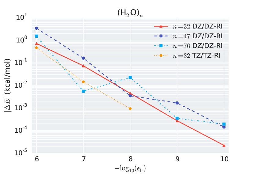
Figure 1: CLR approximation error in the Hartree-Fock energy of water clusters as a function of parameter $\epsilon_{\mathrm{lr}}$ ($\epsilon_{\mathrm{sp}}$=0).

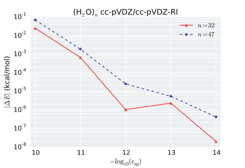
Figure 2: CLR approximation error in the cc-pVDZ Hartree-Fock energy of water clusters as a function of parameter $\epsilon_{\mathrm{sp}}$ ($\epsilon_{\mathrm{lr}}$=0).

Figures 1-6 report the errors in absolute electronic energies and in electric dipole moments relative to the standard DF HF method:

$$|\Delta E| \equiv|E_{\mathrm{CLR}}-E_{\mathrm{ref}}|,$$ (34)

$$|\Delta\boldsymbol{\mu}| \equiv|\,||\boldsymbol{\mu}_{\mathrm{CLR}}||-||\boldsymbol{\mu}_{\mathrm{ref}}||\,|.$$ (35)

As the two CLR thresholds, $\epsilon_{\mathrm{sp}}$ and $\epsilon_{\mathrm{lr}}$ approach zero the error due to CLR should approach zero as well. Figures 1-4 demonstrate that this is indeed the case: the errors decay in proportion to the CLR truncation parameters. Although the errors do not decrease monotonically (e.g. CLR approximation does not guarantee variational character of the energy), the errors can be made arbitrarily small. The errors in energies are all well below the chemical accuracy target. It’s clear that even the most crude threshold values, $\epsilon_{\mathrm{lr}}=10^{-6}$ and $\epsilon_{\mathrm{sp}}=10^{-10}$, will be sufficient for practical chemical applications of hybrid KS DFT. For the rest of the paper we use more stringent values of these parameters, $\epsilon_{\mathrm{lr}}=10^{-8}$ and $\epsilon_{\mathrm{sp}}=10^{-11}$, which should be appropriate for chemical-accuracy evaluation of correlation energies from the Hartree-Fock orbitals and potentials.

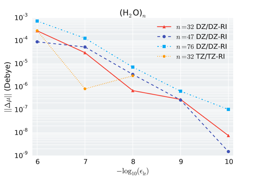
Figure 3: CLR approximation error in the Hartree-Fock dipole moment of water clusters as a function of parameter $\epsilon_{\mathrm{lr}}$ ($\epsilon_{\mathrm{sp}}$=0).

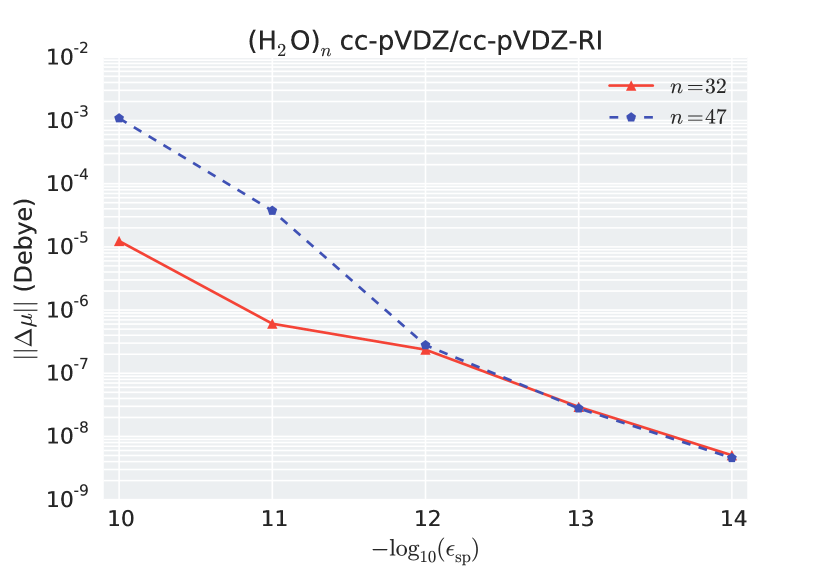
Figure 4: CLR approximation error in the cc-pVDZ Hartree-Fock dipole moment of water clusters as a function of parameter $\epsilon_{\mathrm{sp}}$ ($\epsilon_{\mathrm{lr}}$=0).

Figures 5 and 6 demonstrate the accuracy with regards to system size for the combined approximation. While total error increases with system size, the error per unit for example, while not constant, is controllable and for these calculations is never above $2\times 10^{-4}$ kcal/mol per water molecule or $1.1\times 10^{-3}$ kcal/mol per CH₂ unit in n-alkanes.

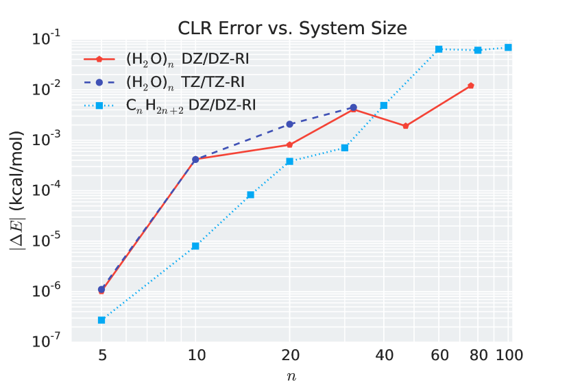
Figure 5: CLR approximation error in the Hartree-Fock energies of water clusters and n-alkanes as a function of system size ($\epsilon_{\mathrm{lr}}=10^{-8},\epsilon_{\mathrm{sp}}=10^{-11}$).

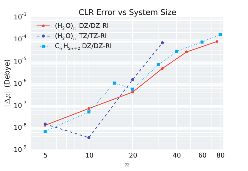
Figure 6: CLR approximation error in the Hartree-Fock dipole moments of water clusters and n-alkanes as a function of system size ($\epsilon_{\mathrm{lr}}=10^{-8},\epsilon_{\mathrm{sp}}=10^{-11}$).

III.3.2 Assessment of Storage Reduction

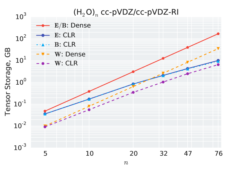
Figure 7: Size (GB) of key order-3 tensors evaluated in density-fitting-based Hartree-Fock method, with and without CLR approximation, as a function of the water cluster size. Basis=cc-pVDZ/cc-pVDZ-RI.

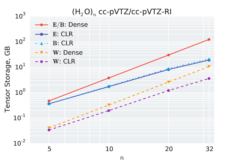
Figure 8: Size (GB) of key order-3 tensors evaluated in density-fitting-based Hartree-Fock method, with and without CLR approximation, as a function of the water cluster size. Basis=cc-pVTZ/cc-pVTZ-RI.

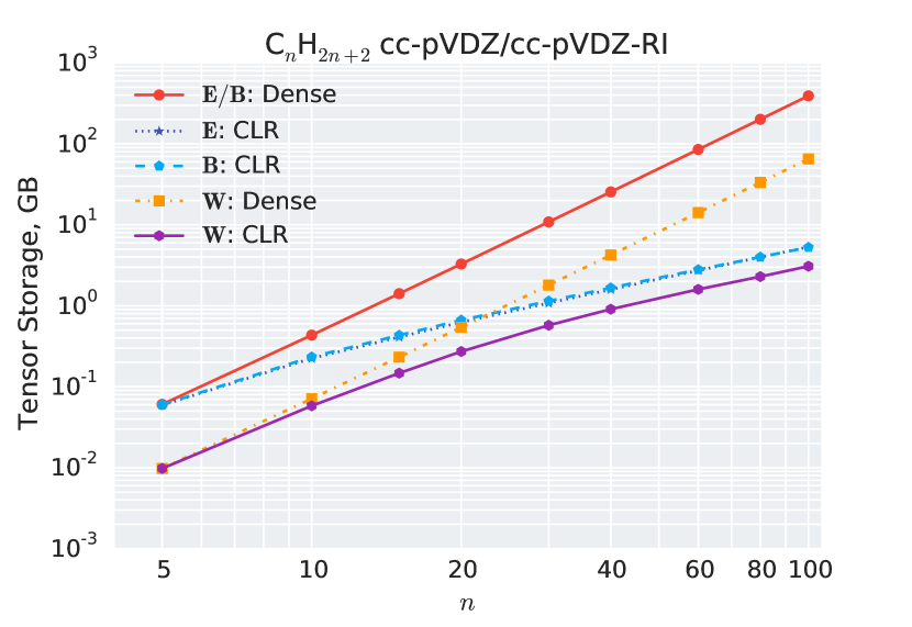
Figure 9: Size (GB) of key order-3 tensors evaluated in density-fitting-based Hartree-Fock method, with and without CLR approximation, as a function of the n-alkane size. Basis=cc-pVDZ/cc-pVDZ-RI.

Figures 7, 8, and 9 show that the use of CLR approximation drastically reduces the data size of order-3 tensors that appear in the DF HF method (storage of the iteration-dependent $\mathbf{W}$ tensor was evaluated after 5 SCF iterations). For example, storage for tensors $\mathbf{E}$ and $\mathbf{B}$ in the double-$\zeta$ basis for (H₂O)₇₆ was reduced, using of CLR, by a factor 16.8 for $\mathbf{E}$ and 18.2 for $\mathbf{B}$. For quasi-1-dimensional C₁₀₀H₂₀₂ these values were 73.6, and 74.3, respectively.

The apparent storage complexity is also significantly reduced compared to $\mathcal{O}\left(N^{3}\right)$ of the standard DF approach. We estimated the effective storage exponent by finite difference from the data for the two largest systems in each series. For n-alkanes the complexity estimates are $\mathcal{O}\left(N^{1.30}\right)$ for $\mathbf{E}$, $\mathcal{O}\left(N^{1.24}\right)$ for $\mathbf{B}$, and $\mathcal{O}\left(N^{1.32}\right)$ for $\mathbf{W}$. Complexity reduction is observed for 3-dimensional systems as well, although they are not as drastic. For example, for water clusters the complexity estimates are $\mathcal{O}\left(N^{1.77}\right)$ and $\mathcal{O}\left(N^{1.82}\right)$ for the $\mathbf{E}$ tensor with the double- and triple-$\zeta$ bases, respectively.

Note that unlike the standard method, in which ratio of storage between tensors $\mathbf{E}$/$\mathbf{B}$ and $\mathbf{W}$ is constant, the CLR storage data reveals that the extent of data sparsity in tensors $\mathbf{E}$ and $\mathbf{B}$ grows faster than in $\mathbf{W}$. Using localized occupied orbitals rather than the Cholesky orbitals can potentially decrease the $\mathbf{W}$ storage further, however detailed investigation of this issue is outside this preliminary investigation.

III.3.3 Performance Assessment

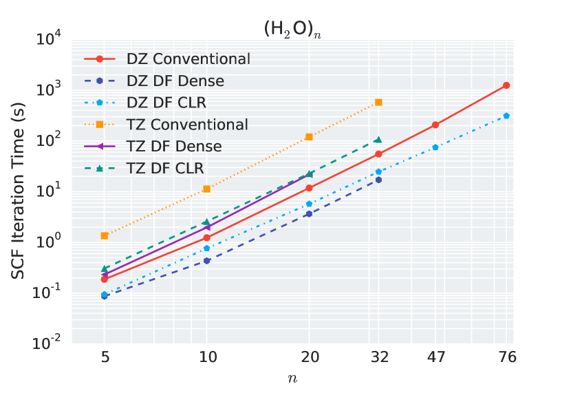
Figure 10: Average SCF iteration times for water clusters. $\epsilon_{\mathrm{sp}}$$=1\times 10^{-11}$ and $\epsilon_{\mathrm{lr}}$$=1\times 10^{-8}$.

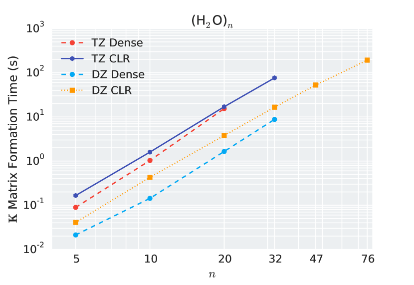
Figure 11: Average exchange build times for water clusters. $\epsilon_{\mathrm{sp}}$$=1\times 10^{-11}$ and $\epsilon_{\mathrm{lr}}$$=1\times 10^{-8}$.

Our implementation supports massive distributed memory parallelism in the Fock matrix build due to the use of TiledArray framework.IA3-TA-paper To simplify the performance assessment here we limited all tests to a single machine with two 8-core Intel Xeon E5-2650 v2 @ 2.60GHz processors and 64 GB of DRAM. Parallel performance, as well as the analysis of performance of block sizes and other parameters will be explored elsewhere.

Figures 10 and 12 show average time per Hartree-Fock SCF iteration for water clusters and n-alkanes obtained with the conventional, DF, and CLR DF approaches (for the former we used the parallel HF test program of Libint library v. 2.1.0-beta). Both standard and CLR DF methods are significantly faster than the conventional counterpart, even when double-$\zeta$ basis sets are used. However, the standard DF approach quickly runs out of the 64 GB RAM: memory allocation becomes problematic around (H₂O)₃₂ and C₄₀H₈₂ in a double-$\zeta$ basis and around (H₂O)₂₀ in a triple-$\zeta$ basis. (conventional DF HF codes of course can avoid this bottleneck by using disk and/or reformulating the exchange build to minimize the storage, but neither strategy reduces the storage complexity to below cubic). Due to the greatly reduced storage requirement much larger computations are possible with the CLR DF method.

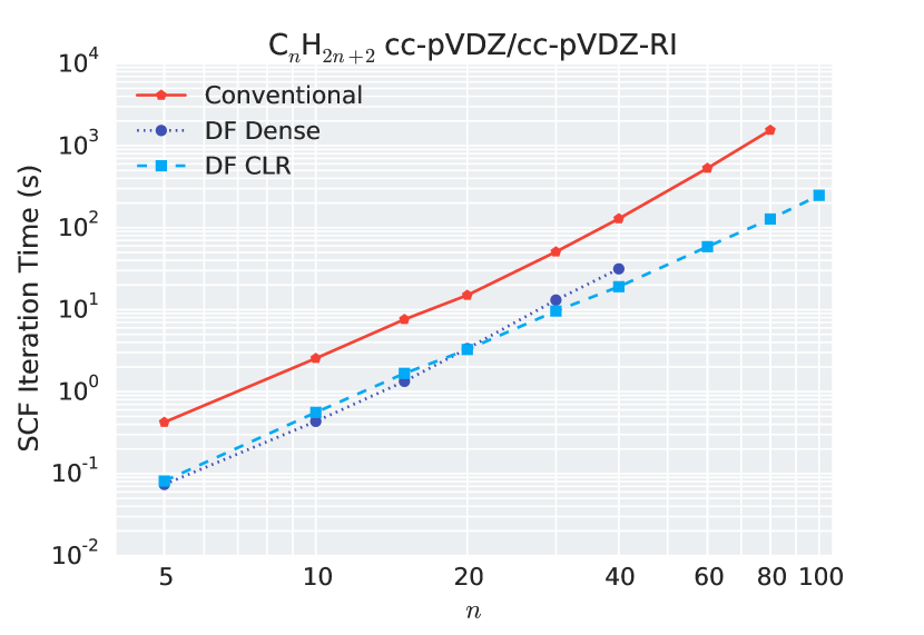
Figure 12: Average SCF iteration times for n-alkanes. $\epsilon_{\mathrm{sp}}$$=1\times 10^{-11}$ and $\epsilon_{\mathrm{lr}}$$=1\times 10^{-8}$.

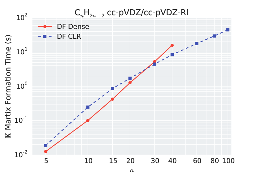
Figure 13: Average exchange build times for n-alkanes. $\epsilon_{\mathrm{sp}}$$=1\times 10^{-11}$ and $\epsilon_{\mathrm{lr}}$$=1\times 10^{-8}$.

Most importantly, for n-alkanes in a double-$\zeta$ basis CLR DF HF becomes faster than its standard DF HF counterpart, due to lower computational complexity. This is best demonstrated when considering timings for the most expensive step only, namely the exchange matrix construction (this includes computation of $\mathbf{W}$ and $\mathbf{K}$ matrices). Figure 13 demonstrates that for double-$\zeta$ alkanes the CLR-based method becomes faster than the standard counterpart between 20 and 30 carbon atoms. For the triple-$\zeta$ water clusters the crossover occurs around 20 water molecules; for the double-$\zeta$ basis the crossover does not occur, but due to the smaller slope of the CLR line the cross-over is bound to occur for a larger system, with more than 50 water molecules.

We estimated the effective computational complexity of the exchange construction using the finite difference from the two data points for the largest systems in each series. For water clusters and n-alkanes in a double-$\zeta$ basis the observed complexities is $\mathcal{O}\left(N^{2.7}\right)$ and $\mathcal{O}\left(N^{1.86}\right)$, respectively, and for water clusters in a triple-$\zeta$ basis the complexity is $\mathcal{O}\left(N^{3.2}\right)$. All of these figures compare favorably to the $\mathcal{O}\left(N^{4}\right)$ complexity of the standard DF exchange algorithm.

IV Conclusions and Perspective

In this work we introduced the Clustered Low Rank (CLR) framework for block-sparse and block-low-rank tensor representation and computation. Use of the CLR format for the order-2 and order-3 tensors that appear in the context of density-fitting-based Hartree-Fock method significantly reduced the storage and computational complexities below their standard $\mathcal{O}\left(N^{3}\right)$ and $\mathcal{O}\left(N^{4}\right)$ figures. Even for relatively small systems and realistic basis sets CLR-based DF HF becomes more efficient than the standard DF approach while negligibly affecting molecular energies and properties.

The entire computation framework that we described here depends on 2 parameters that control precision. Precision of the CLR representation depends on input parameter that controls the block rank truncation; as it approaches 0 the representation becomes exact. Another parameter controls screening of small contributions in arithmetic operations on CLR tensors; as it approaches 0 the arithmetic becomes exact. There are no other ad-hoc heuristics, such as domains.

This is an initial application of the CLR format, and many significant optimization opportunities remain to be explored. Nevertheless, the efficiency of CLR DF HF method immediately makes it useful on its own and as a building block for other reduced scaling methods. For example, the fast CLR-based DF methodology should also be immediately applicable in other contexts where density fitting is key, e.g. the reduced scaling electron correlation methods. The high efficiency of the CLR DF Fock build suggests that the analytic gradients for CLR-based hybrid KS DFT is a logical next step, to allow efficient on-the-fly dynamics. We should note that the CLR framework should be naturally beneficial for massive parallelism necessary for ab initio dynamics, since the CLR data compression should reduce the traffic through the memory hierarchy, whether between memory tiers in the next generation of “accelerators” or through the network in a cluster.

Last, but not least, it is exciting to imagine uses of the CLR framework for exploiting the data sparsity in other tensors that appear in electronic structure and related fields, such as the wave function projections (e.g. cluster amplitudes), density matrices and Green’s functions. Some work along these lines is already underway.

V Acknowledgements

We would like to thank Fabijan Pavošević for useful discussions and Virginia Tech’s Advanced Research Computing for providing time on BlueRidge cluster, which was used for debugging and obtaining reference values for large dense calculations. We acknowledge the support by the U.S. National Science Foundation (grants CHE-1362655 and ACI-1450262), and by Camille and Henry Dreyfus Foundation.

References

- (1) A. Tajti, P. G. Szalay, A. G. Császár, M. Kállay, J. Gauss, E. F. Valeev, B. A. Flowers, J. Vázquez, and J. F. Stanton, J. Chem. Phys. 121, 11599 (2004).
- (2) Y. J. Bomble, J. Vázquez, M. Kállay, C. Michauk, P. G. Szalay, A. G. Császár, J. Gauss, and J. F. Stanton, J. Chem. Phys. 125, 064108 (2006).
- (3) M. E. Harding, J. Vázquez, B. Ruscic, A. K. Wilson, J. Gauss, and J. F. Stanton, J. Chem. Phys. 128, 114111 (2008).
- (4) T. Shiozaki, E. F. Valeev, and S. Hirata, J. Chem. Phys. 131, 044118 (Jul. 2009).
- (5) G. H. Booth, A. Grüneis, G. Kresse, and A. Alavi, Nature 493, 365 (Jan. 2013).
- (6) J. Yang, W. Hu, D. Usvyat, D. Matthews, M. Schütz, and G. K.-L. Chan, Science 345, 640 (Aug. 2014).
- (7) G. E. Scuseria, C. L. Janssen, and H. F. Schaefer, J. Chem. Phys. 89, 7382 (1988).
- (8) R. J. Bartlett, Annu. Rev. Phys. Chem. 32, 359 (Oct. 1981).
- (9) P. V. Strassen, Numer. Math. 13, 354 (1969).
- (10) L. Greengard and V. Rokhlin, J. Comp. Phys. 73, 325 (Dec. 1987).
- (11) C. A. White, B. G. Johnson, P. M. W. Gill, and M. Head-Gordon, Chem. Phys. Letters 230, 8 (Nov. 1994).
- (12) W. Kohn, Phys. Rev. Lett. 76, 3168 (Apr. 1996).
- (13) X. P. Li, R. W. Nunes, and D. Vanderbilt, Phys. Rev. B 47, 10891 (Apr. 1993).
- (14) J. M. Millam and G. E. Scuseria, J. Chem. Phys. 106, 5569 (1997).
- (15) C. Ochsenfeld and J. Kussmann, Rev. Comp. Chem. 23, 1. (2007).
- (16) A. Niklasson and C. J. Tymczak, J. Chem. Phys 118, 8611 (2003).
- (17) Y. Shao, C. Saravanan, and M. Head-Gordon, J. Chem. Phys 118, 6144 (2003).
- (18) M. Challacombe, J. Chem. Phys. 110, 2332 (1999).
- (19) A. Palser and D. E. Manolopoulos, Phys. Rev. B 58, 12704 (1998).
- (20) E. Rudberg, E. H. Rubensson, and P. Sałek, J. Chem. Phys. 128, 184106 (May 2008).
- (21) E. Rudberg, E. H. Rubensson, and P. Sałek, J. Chem. Theory Comput. 7, 340 (Feb. 2011).
- (22) J. VandeVondele, U. Borštnik, and J. Hutter, J. Chem. Theory Comput. 8, 3565 (Mar. 2012).
- (23) G. E. Scuseria and P. Y. Ayala, J. Chem. Phys. 111, 8330 (Nov. 1999).
- (24) F. Neese, F. Wennmohs, and A. Hansen, J. Chem. Phys. 130, 114108 (2009).
- (25) C. Riplinger and F. Neese, J. Chem. Phys. 138, 034106 (2013).
- (26) P. Pinski, C. Riplinger, E. F. Valeev, and F. Neese, J. Chem. Phys. 143, 034108 (Jul. 2015).
- (27) R. Vandebril, M. Van Barel, G. Golub, and N. Mastronardi, Calcolo 42, 249 (2005).
- (28) S. Chandrasekaran, P. Dewilde, M. Gu, T. Pals, X. Sun, A. J. van der Veen, and D. White, SIAM. J. Matrix Anal. & Appl. 27, 341 (Jan. 2005).
- (29) J. Xia, S. Chandrasekaran, M. Gu, and X. S. Li, Numer. Linear Algebra Appl. 17, 953 (Dec. 2010).
- (30) W. Hackbusch, Computing 62, 89 (1999).
- (31) W. Hackbusch and B. N. Khoromskij, Computing 64, 21 (2000).
- (32) L. Grasedyck and W. Hackbusch, Computing 70, 295 (2003).
- (33) N. Bock and M. Challacombe, SIAM J. Sci. Comput. 35, C72 (2013).
- (34) P. Benner, V. Khoromskaia, and B. N. Khoromskij, arXiv preprint arXiv:1505.02696 [math.NA](2015).
- (35) V. Rokhlin, J. Comp. Phys. 60, 187 (Sep. 1985).
- (36) W. Hackbusch and Z. P. Nowak, Numer. Math. 54, 463 (1989).
- (37) E. Tyrtyshnikov, Calcolo 33, 47 (Jun. 1996).
- (38) E. Tyrtyshnikov, in Numerical Analysis and Its Applications, Lecture Notes in Computer Science, Vol. 1196, edited by L. Vulkov, J. Waśniewski, and P. Yalamov (Springer Berlin Heidelberg, 1997) pp. 505–516, ISBN 978-3-540-62598-8, http://dx.doi.org/10.1007/3-540-62598-4_132.
- (39) S. A. Goreinov, E. E. Tyrtyshnikov, and N. L. Zamarashkin, Linear Algebra and its Applications 261, 1 (Aug. 1997).
- (40) V. Weber, T. Laino, A. Pozdneev, I. Fedulova, and A. Curioni, J. Chem. Theory Comput. 11, 3145 (Jul. 2015).
- (41) E. Schwegler and M. Challacombe, J Chem Phys 105, 2726 (1996).
- (42) J. C. Burant, G. E. Scuseria, and M. J. Frisch, J Chem Phys 105, 8969 (1996).
- (43) C. Ochsenfeld, C. A. White, and M. Head-Gordon, J. Chem. Phys. 109, 1663 (1998).
- (44) F. Neese, F. Wennmohs, A. Hansen, and U. Becker, Chemical Physics 356, 98 (Feb. 2009).
- (45) S. P. Lloyd, IEEE Transactions on Information Theory 28, 129 (Mar. 1982).
- (46) A. K. Jain, Pattern Recognition Letters 31, 651 (Jun. 2010).
- (47) D. Arthur and S. Vassilvitskii, in Proceedings of the eighteenth annual ACM-SIAM symposium on Discrete algorithms (Society for Industrial and Applied Mathematics, 2007) pp. 1027–1035.
- (48) D. S. Hollman, H. F. Schaefer, and E. F. Valeev, J. Chem. Phys. 142, 154106 (Apr. 2015).
- (49) T. F. Chan, Linear Algebra and its Applications 88-89, 67 (1987).
- (50) G. Quintana-Ortí, X. Sun, and C. H. Bischof, SIAM J. Sci. Comput. 19, 1486 (1998).
- (51) C. H. Bischof and G. Quintana-Ortí, ACM Transactions on Mathematical Software (TOMS) 24, 226 (Jun. 1998).
- (52) J. L. Whitten, J. Chem. Phys. 58, 4496 (1973).
- (53) E.-J. Baerends, D. E. Ellis, and P. Ros, Chem. Phys. 2, 41 (1973).
- (54) M. Feyereisen, G. Fitzgerald, and A. Komornicki, Chem. Phys. Letters 208, 359 (1993).
- (55) O. Vahtras, J. Almlöf, and M. W. Feyereisen, Chem. Phys. Letters 213, 514 (1993).
- (56) B. I. Dunlap, Journal of Molecular Structure: THEOCHEM 529, 37 (Sep. 2000).
- (57) R. A. Kendall and H. A. Früchtl, Theoret. Chim. Acta 97, 158 (Oct. 1997).
- (58) R. T. Gallant and A. St-Amant, Chem. Phys. Letters 256, 569 (1996).
- (59) C. F. Guerra, J. G. Snijders, and G. te Velde, Theor. Chem. Acc. 99, 391 (1998).
- (60) M. A. Watson, N. C. Handy, and A. J. Cohen, J. Chem. Phys. 119, 6475 (2003).
- (61) P. Merlot, T. Kjærgaard, and T. Helgaker, J. Comput. Chem 34, 1486 (2013).
- (62) D. S. Hollman, H. F. Schaefer, and E. F. Valeev, J. Chem. Phys. 140, 064109 (Feb. 2014).
- (63) S. Manzer, P. R. Horn, N. Mardirossian, and M. Head-Gordon, J. Chem. Phys. 143, 024113 (Jul. 2015).
- (64) F. Aquilante, T. B. Pedersen, A. S. de Merás, and H. Koch, J. Chem. Phys. 125, 174101 (Nov. 2006).
- (65) J. A. Calvin and E. F. Valeev, “Tiledarray: A massively-parallel, block-sparse tensor library written in C++ ,” https://github.com/valeevgroup/tiledarray/ (2015).
- (66) N. M. O’Boyle, M. Banck, C. A. James, C. Morley, T. Vandermeersch, and G. R. Hutchison, J. Cheminf. 3, 33 (Oct. 2011).
- (67) http://www.ergoscf.org/xyz/h2o.php, accessed : 2015-08-10.
- (68) T. H. Dunning, J. Chem. Phys. 90, 1007 (1989).
- (69) F. Weigend, A. Köhn, and C. Hättig, J. Chem. Phys. 116, 3175 (Feb. 2002).
- (70) Note that due to the lack of support for permutational symmetry in TiledArray (the feature is under current development) the storage size for both and is twice what it should be in practice, however this deficiency does not affect the storage comparison between CLR and standard DF.
- (71) J. A. Calvin, C. A. Lewis, and E. F. Valeev, “Scalable Task-Based Algorithm for Multiplication of Block-Rank-Sparse Matrices,” (Aug. 2015), accepted to Proceedings of IA3 2015: 5th Workshop on Irregular Applications: Architectures and Algorithms, arXiv:1509.00309.