Balancing the Communication Load of Asynchronously Parallelized Machine Learning Algorithms

Abstract

Stochastic Gradient Descent (SGD) is the standard numerical method used to solve the core optimization problem for the vast majority of machine learning (ML) algorithms. In the context of large scale learning, as utilized by many Big Data applications, efficient parallelization of SGD is in the focus of active research.
Recently, we were able to show that the asynchronous communication paradigm can be applied to achieve a fast and scalable parallelization of SGD. Asynchronous Stochastic Gradient Descent (ASGD) outperforms other, mostly MapReduce based, parallel algorithms solving large scale machine learning problems.
In this paper, we investigate the impact of asynchronous communication frequency and message size on the performance of ASGD applied to large scale ML on HTC cluster and cloud environments. We introduce a novel algorithm for the automatic balancing of the asynchronous communication load, which allows to adapt ASGD to changing network bandwidths and latencies.

1 Introduction

The enduring success of Big Data applications, which typically includes the mining, analysis and inference of very large datasets, is leading to a change in paradigm for machine learning research objectives [4]. With plenty data at hand, the traditional challenge of inferring generalizing models from small sets of available training samples moves out of focus. Instead, the availability of resources like CPU time, memory size or network bandwidth has become the dominating limiting factor for large scale machine learning algorithms.
In this context, algorithms which guarantee useful results even in the case of an early termination are of special interest. With limited (CPU) time, fast and stable convergence is of high practical value, especially when the computation can be stopped at any time and continued some time later when more resources are available.
Parallelization of machine learning (ML) methods has been a rising topic for some time (refer to [1] for a comprehensive overview). Most current approaches rely on the MapReduce pattern. It has been shown [5], that most of the existing ML techniques could easily be transformed to fit the MapReduce scheme. However, it is also known [11], that MapReduce’s easy parallelization comes at the cost of potentially poor scalability. The main reason for this undesired behavior resides deep down within the numerical properties most machine learning algorithms have in common: an optimization problem. In this context, MapReduce works very well for the implementation of so called batch-solver approaches, which were also used in the MapReduce framework of [5]. However, batch-solvers have to run over the entire dataset to compute a single iteration step. Hence, their scalability with respect to the data size is obviously poor.
Therefore, even most small scale ML implementations avoid the known drawbacks of batch-solvers by usage of alternative online optimization methods. Most notably, Stochastic Gradient Descent (SGD) methods have long proven to provide good results for ML optimization problems [11].
However, due to its inherent sequential nature, SGD is hard to parallelize and even harder to scale [11]. Especially, when communication latencies are causing dependency locks, which is typical for parallelization tasks on distributed memory systems [13].

In [8], we introduced a lock-free parallelization method for the computation of stochastic gradient optimization of large scale machine learning algorithms, which is based on the asynchronous communication paradigm. Figure 1 displays the key results of [8], showing that Asynchronous Stochastic Gradient Descent (ASGD) outperforms both batch and online algorithms in terms of convergence speed, scalability and prediction error rates.

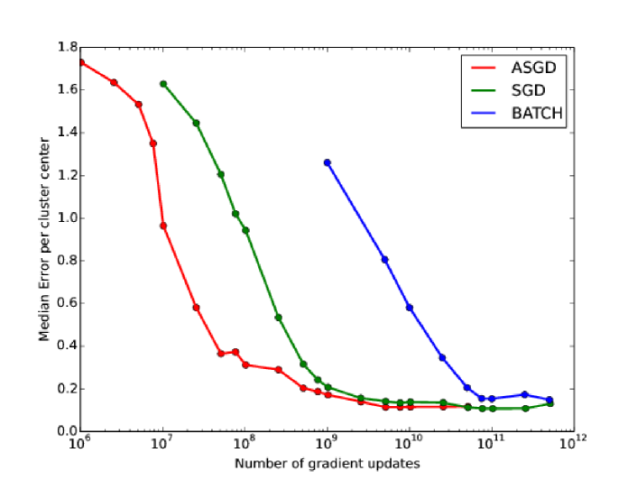
Figure 1: LEFT:Convergence speed of different gradient descent methods used to solve K-Means clustering with $K=100$ on a $10$-dimensional target space parallelized over $1024$ cores on a cluster. The ASGD method outperforms communication free SGD [13] and MapReduce based BATCH [5] optimization by the order of a magnitude. RIGHT: Scaling properties of the same experiment: ASGD is not only faster than SGD and BATCH, it also provides linear strong scaling in the number of CPUs, while SGD suffers from increasing communication overheads. See [8] for detailed evaluations.

In this paper, we extend the ASGD by an algorithm which automatically sets the communication and update frequencies. These are key parameters which have a large impact on the convergence performance. In [8], they were set experimentally. However, they optimal choice is subject to a large number of factors and influenced by the computing environment: interconnection bandwidth, number nodes, cores per node, or NUMA layout, just to name a few. Hence, for a heterogeneous setup (e.g. in the Cloud) it is hardly possible to determine a globally optimal set of parameters. We therefore introduce a adaptive algorithm, which choses the parameters dynamically during the runtime of ASGD.

1.1 Related Work

Recently, several approaches towards an effective parallelization of the SGD optimization have been proposed. A detailed overview and in-depth analysis of their application to machine learning can be found in [13].
In this section, we focus on a brief discussion of related publications, which provided the essentials for the ASGD approach:

• A theoretical framework for the analysis of SGD parallelization performance has been presented in [13]. The same paper also introduced a novel approach (called SimuParallelSGD), which avoids communication and any locking mechanisms up to a single and final MapReduce step.

• A widely noticed approach for a “lock-free” parallelization of SGD on shared memory systems has been introduced in [11]. The basic idea of this method is to explicitly ignore potential data races and to write updates directly into the memory of other processes. Given a minimum level of sparsity, they were able to show that possible data races will neither harm the convergence nor the accuracy of a parallel SGD. Even more, without any locking overhead, [11] sets the current performance standard for shared memory systems.

• In [6], the concept of a Partitioned Global Address Space programming framework (called GASPI) has been introduced. This provides an asynchronous, single-sided communication and parallelization scheme for cluster environments. We build our asynchronous communication on the basis of this framework.

2 The Machine Learning Optimization Problem

From a strongly simplified perspective, machine learning tasks are usually solving the problem of inferring generalized models from a given dataset $X=\{x_{0},\dots,x_{m}\}$ with $x_{i}\in\mathbb{R}^{n}$, which in case of supervised learning is also assigned with semantic labels $Y=\{y_{0},\dots,y_{m}\},y_{i}\in\mathbb{R}$. During the learning process, the quality of a model is evaluated by use of so-called loss-functions, which measure how well the current model represents the given data. We write $x_{j}(w)$ or $(x_{j},y_{j})(w)$ to indicate the loss of a data point for the current parameter set $w$ of the model function. We will also refer to $w$ as the “state” of the model. The actual learning is then the process of minimizing the loss over all samples. This is usually done by a gradient descent over the partial derivative of the loss function in the parameter space of $w$.

Stochastic Gradient Descent.

Although some properties of Stochastic Gradient Descent approaches might prevent their successful application to some optimization domains, they are well established in the machine learning community [2].

Algorithm 1 SGD with samples $X=\{x_{0},\dots,x_{m}\}$, iterations $T$, steps size $\epsilon$ and states $w$

1:$\epsilon>0$

2:for all $t=0\dots T$  do

3:     draw $j\in\{1\dots m\}$ uniformly at random

4:     update $w_{t+1}\leftarrow w_{t}-\epsilon\partial_{w}x_{j}(w_{t})$

5:return $w_{T}$

Following the notation in [13], SGD can be formalized in pseudo code as outlined in algorithm 1. For further simplification, we will write $\Delta_{j}(w_{t}):=\partial_{w}x_{j}(w_{t})$ for the remainder of this paper.

2.1 Asynchronous SGD

The basic idea of the ASGD algorithm is to port the “lock-free” shared memory approach from [11] to distributed memory systems. This is far from trivial, mostly because communication latencies in such systems will inevitably cause expensive dependency locks if the communication is performed in common two-sided protocols (such as MPI message passing or MapReduce). This is also the motivation for SimuParallelSGD [13] to avoid communication during the optimization: locking costs are usually much higher than the information gain induced by the communication.
We overcome this dilemma by the application of the asynchronous, single-sided communication model provided by [6]: individual processes send mini-BATCH [12] updates completely uninformed of the recipients status whenever they are ready to do so. On the recipient side, available updates are included in the local computation as available. In this scheme, no process ever waits for any communication to be sent or received. Hence, communication is literally “free” (in terms of latency).
Of course, such a communication scheme will cause data races and race conditions: updates might be (partially) overwritten before they were used or even might be contra productive because the sender state is way behind the state of the recipient.
ASGD solves these problems by two strategies: first, we obey the sparsity requirements introduced by [11]. This can be achieved by sending only partial updates to a few random recipients. Second, we introduced a Parzen-window function, selecting only those updates for local descent which are likely to improve the local state. ASGD is formalized and implemented on the basis of the SGD parallelization presented in [13]. In fact, the asynchronous communication is just added to the existing approach. This is based on the assumption that communication (if performed correctly) can only improve the gradient descent - especially when it is “free”. If the communication interval is set to infinity, ASGD will become SimuParallelSGD.

Implementation.

Our ASGD implementation is based on the open-source library GPI 2.0, which provides a C++ interface to the GASPI specification.

Parameters.

ASGD takes several parameters, which can have a strong influence on the convergence speed and quality: $\bf T$ defines the size of the data partition for each thread, $\bf\epsilon$ sets the gradient step size (which needs to be fixed following the theoretic constraints shown in [13]), $\bf b$ sets the size of the mini-batch aggregation, and $\bf I$ gives the number of SGD iterations for each thread. Practically, this also equals the number of data points touched by each thread.

Initialization.

The initialization step is straight forward and analog to SimuParallelSGD [13] : the data is split into working packages of size $T$ and distributed to the worker threads. A control thread generates initial, problem dependent values for $w_{0}$ and communicates $w_{0}$ to all workers. From that point on, all workers run independently. It should be noted, that $w_{0}$ also could be initialized with the preliminary results of a previously early terminated optimization run.

Updating.

The online gradient descent update step is the key leverage point of the ASGD algorithm. The local state $w^{i}_{t}$ of thread $i$ at iteration $t$ is updated by an externally modified step $\overline{\Delta_{t}(w^{i}_{t+1})}$, which not only depends on the local $\Delta_{t}(w^{i}_{t+1})$ but also on a possible communicated state $w^{j}_{t^{\prime}}$ from an unknown iteration $t^{\prime}$ at some random thread $j$:

$$\overline{\Delta_{t}(w^{i}_{t+1})}=w^{i}_{t}-{1\over 2}\left(w^{i}_{t}+w^{j}_{t^{\prime}}\right)+\Delta_{t}(w^{i}_{t+1})$$ (1)

Figure 2 gives a schematic overview of the update process.

Parzen-Window Optimization.

As discussed before, the asynchronous communication scheme is prone to cause data races and other conditions during the update. Hence, we introduced a Parzen-window like function $\delta(i,j)$ to avoid “bad” update conditions. The handling of data races is discussed in [8].

$$\delta(i,j):=\left\{\begin{tabular}[]{ll}$1$&if $\|(w^{i}_{t}-\epsilon\Delta w^{i}_{t})-w^{j}_{t^{\prime}}\|^{2}<\|w^{i}_{t}-w^{j}_{t^{\prime}}\|^{2}$\\ $0$&otherwise\end{tabular}\right.,$$ (2)

We consider an update to be “bad”, if the external state $w^{j}_{t^{\prime}}$ would direct the update away from the projected solution, rather than towards it. Figure 2 shows the evaluation of $\delta(i,j)$, which is then plugged into the update functions of ASGD in order to exclude undesirable external states from the computation. Hence, equation (1) turns into

$$\overline{\Delta_{t}(w^{i}_{t+1})}=\left[w^{i}_{t}-{1\over 2}\left(w^{i}_{t}+w^{j}_{t^{\prime}}\right)\right]\delta(i,j)+\Delta_{t}(w^{i}_{t+1})$$ (3)

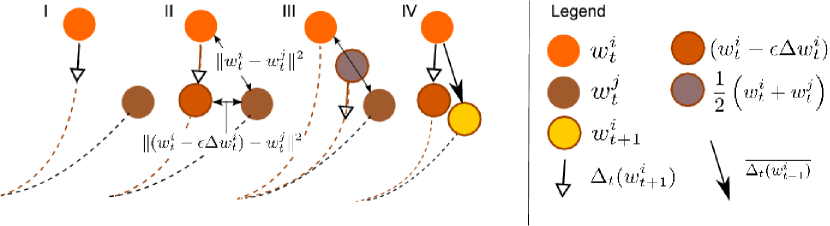
Figure 2: ASGD updating. This figure visualizes the update algorithm of a process with state $w^{i}_{t}$, its local mini-batch update $\Delta_{t}(w^{i}_{t+1})$ and received external state $w^{j}_{t}$ for a simplified 1-dimensional optimization problem. The dotted lines indicate a projection of the expected descent path to an (local) optimum. I: Initial setting: ${\bf\Delta}_{M}(w^{i}_{t+1})$ is computed and $w^{j}_{t}$ is in the external buffer. II: Parzen-window masking of $w^{j}_{t}$. Only if the condition of equation (2) is met, $w^{j}_{t}$ will contribute to the local update. III: Computing $\overline{{\bf\Delta}_{M}(w^{i}_{t+1})}$. IV: Updating $w^{i}_{t+1}\leftarrow w^{i}_{t}-\epsilon\overline{{\bf\Delta}_{M}(w^{i}_{t+1})}$.

In addition to the Parzen-window, we also introduced a mini-batch update in [8]: instead of updating after each step, several updates are aggregated into mini-batches of size $b$. We are writing ${\bf\Delta}_{M}$ in order to differentiate mini-batch steps from single sample steps $\Delta_{t}$ of sample $x_{t}$:

$$\overline{{\bf\Delta}_{M}(w^{i}_{t+1})}=\left[w^{i}_{t}-{1\over 2}\left(w^{i}_{t}+w^{j}_{t}\right)\right]\delta(i,j)+{\bf\Delta}_{M}(w^{i}_{t+1})$$ (4)

Computational Costs of Communication.

Obviously, the evaluation of $\delta(i,j)$ comes at some computational cost. Since $\delta(i,j)$ has to be evaluated for each received message, the “free” communication is actually not so free after all. However, the costs are very low and can be reduced to the computation of the distance between two states, which can be achieved linearly in the dimensionality of the parameter-space of $w$ and the mini-batch size: $O({1\over b}|w|)$. In practice, the communication frequency ${1\over b}$ is mostly constrained by the network bandwidth and latency between the compute nodes, which is subject to our proposed automatic adaption algorithm in the next section. 3.

The ASGD Algorithm.

Following [8], the final ASGD algorithm with mini-batch size $b$, number of iterations $I$ and learning rate $\epsilon$ can be implemented as shown in algorithm 2.

Algorithm 2 ASGD $(X=\{x_{0},\dots,x_{m}\},T,\epsilon,w_{0},b)$

1:$\epsilon>0,n>1$

2:define $H=\lfloor{m\over n}\rfloor$

3:randomly partition $X$, giving $H$ samples to each node

4:for all $i\in\{1,\dots,n\}$ parallel  do

5:     randomly shuffle samples on node $i$

6:     init $w^{i}_{0}=0$

7:     for all $t=0\dots T$  do

8:         draw mini-batch $M\leftarrow b$ samples from $X$

9:         update $w^{i}_{t+1}\leftarrow w^{i}_{t}-\epsilon\overline{{\bf\Delta}_{M}(w^{i}_{t+1})}$

10:         send $w^{i}_{t+1}$ to random node $\neq i$      

11:return $w^{1}_{I}$

At termination, all nodes $w^{i},i\in\{1,\dots,n\}$ hold small local variations of the global result. We simply return one of these (namely $w^{1}_{I}$). Experiments showed, that further aggregation of the $w^{i}_{I}$ (via map reduce) provides no improvement of the results and can be neglected.

3 Communication load balancing

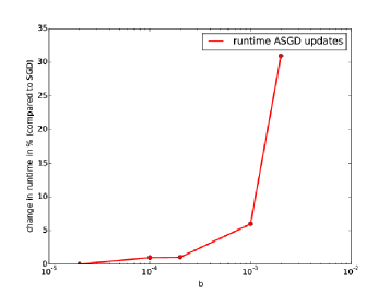
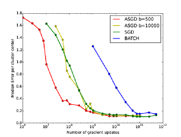
Figure 3: LEFT: Communication cost of ASGD. The cost of higher communication frequencies $1\over b$ in ASGD updates compared to communication free SGD updates. RIGHT: Convergence speed of ASGD with a communication frequencies of $1\over 100000$ compared to $1\over 500$ in relation to the other methods. Results on Synthetic data with $D=10,K=100$.

The impact of the communication frequencies of $1\over b$ on the convergence properties of ASGD are displayed in figure 3. If the frequency is set to lower values, the convergence moves towards the original SimuParallelSGD behavior. The results in Figure 3 show that the choice of the communication frequency ${1\over b}$ has a significant impact on the convergence speed. Theoretically, more communication should be beneficial. However, due to the limited bandwidth, the practical limit is expected to be far from $b=1$.
The choice of an optimal $b$ strongly depends on the data (in terms of dimensionality) and the computing environment: interconnection bandwidth and latency, number of nodes, cores per node, NUMA layout and so on.
In [8], the ASGD approach has only been tested in an HPC cluster environment with Infiniband interconnections, where neither bandwidth nor latency issues were found to have significant effect on the experiments. Hence, $b$ was set to a fixed value which has been selected experimentally.
However, for most Big Data applications, especially in HTC environments like the cloud, Infiniband networks are not very common. Instead, one usually has to get along with Gigabit-Ethernet connections, which even might suffer from external traffic. Figures 5 and 6 show the effect of reduced bandwidth and higher latencies on the ASGD performance: As one can expect, the number of messages that can be passed through the network, underlies stronger bounds compared to Infiniband. Notably, our experiments indicate, that there appears to be a clear local optimum for $b$, where the number of messages correlates to the available bandwidth. Because this local optimum might even change during runtime (through external network traffic) and a full series of experiments on large datasets (in order to determine $b$) is anything but practical, we propose an adaptive algorithm which regulates $b$ during the runtime of ASGD.

3.1 Adaptive optimal $b$ estimation

The GPI2.0 interface allows the monitoring of outgoing asynchronous communication queues. By keeping a small statistic over the past iterations, our approach dynamically increases the frequency $1\over b$ when queues are running low, and decreases or holds otherwise. Algorithm 3 is run on all nodes independently, dynamically setting $b$ for all local threads.

Algorithm 3 adaptiveB $(q_{opt},q_{0},q_{1},q_{2},\gamma)$

1:get current queue state $q_{0}$

2:compute gradient $\Delta_{q}=(q_{opt}-q_{0})-(q_{2}-q_{0})$

3:update $b=b-\Delta_{q}*\gamma$

4:update history $q_{2}=q1,q_{1}=q_{0}$

5:return $b$

Where $q_{0}$ is the current queue size queried from the GPI interface, $q_{opt}$ the target queue size, $q_{1},q_{2}$ the queue history and $\gamma$ the step size regularisation.

4 Experiments

We evaluate the performance of our proposed method in terms of convergence speed, scalability and error rates of the learning objective function using the K-Means Clustering algorithm. The motivation to choose this algorithm for evaluation is twofold: First, K-Means is probably one of the simplest machine learning algorithms known in the literature (refer to [7] for a comprehensive overview). This leaves little room for algorithmic optimization other than the choice of the numerical optimization method. Second, it is also one of the most popular unsupervised learning algorithms with a wide range of applications and a large practical impact.

4.1 K-Means Clustering

K-Means is an unsupervised learning algorithm, which tries to find the underlying cluster structure of an unlabeled vectorized dataset. Given a set of $m$ $n$-dimensional points $X=\{x_{i}\},i=1,\dots,m$, which is to be clustered into a set of $k$ clusters, $w=\{w_{k}\},k=1,\dots,k$. The K-Means algorithm finds a partition such that the squared error between the empirical mean of a cluster and the points in the cluster is minimized.
It should be noted, that finding the global minimum of the squared error over all $k$ clusters $E(w)$ is proven to be a NP-HARD problem [7]. Hence, all optimization methods investigated in this paper are only approximations of an optimal solution. However, it has been shown [10], that K-Means finds local optima which are very likely to be in close proximity to the global minimum if the assumed structure of $k$ clusters is actually present in the given data.

Gradient Descent Optimization

Following the notation given in [3], K-Means is formalized as minimization problem of the quantization error $E(w)$:

$$E(w)=\sum_{i}{1\over 2}(x_{i}-w_{s_{i}(w)})^{2},$$ (5)

where $w=\{w_{k}\}$ is the target set of $k$ prototypes for given $m$ examples $\{x_{i}\}$ and $s_{i}(w)$ returns the index of the closest prototype to the sample $x_{i}$. The gradient descent of the quantization error $E(w)$ is then derived as $\Delta(w)={\partial E(w)\over\partial w}$. For the usage with the previously defined gradient descent algorithms, this can be reformulated to the following update function with step size $\epsilon$.

$$\Delta(w_{k})=\left\{\begin{tabular}[]{ll}$x_{i}-w_{k}$&if $k=s_{i}(w)$\\ $0$&otherwise\end{tabular}\right.$$ (6)

4.2 Setup

The experiments were conducted on a Linux cluster with a BeeGFS parallel file system. Each compute node is equipped with dual Intel Xeon E5-2670, totaling to 16 cores per node, 32 GB RAM and interconnected with FDR Infiniband or Gigabit-Ethernet. If not noted otherwise, we used a standard of 64 nodes to compute the experimental results (which totals to 1024 CPUs).

Synthetic Data Sets

The need to use synthetic datasets for evaluation arises from several rather profound reasons: (I) the optimal solution is usually unknown for real data, (II) only a few very large datasets are publicly available, and, (III) we even need a collection of datasets with varying parameters such as dimensionality $n$, size $m$ and number of clusters $k$ in order to evaluate the scalability.
The generation of the data follows a simple heuristic: given $n,m$ and $k$ we randomly sample $k$ cluster centers and then randomly draw $m$ samples. Each sample is randomly drawn from a distribution which is uniquely generated for the individual centers. Possible cluster overlaps are controlled by additional minimum cluster distance and cluster variance parameters. The detailed properties of the datasets are given in the context of the experiments.

Evaluation

Due to the non-deterministic nature of stochastic methods and the fact that the investigated K-Means algorithms might get stuck in local minima, we apply a 10-fold evaluation of all experiments. If not noted otherwise, plots show the median results. Since the variance is usually magnitudes lower than the plotted scale, we neglect the display of variance bars in the plots for the sake of readability.
Errors reported for the synthetic datasets are computed as follows: We use the “ground-truth” cluster centers from the data generation step to measure their distance to the centers returned by the investigated algorithms.

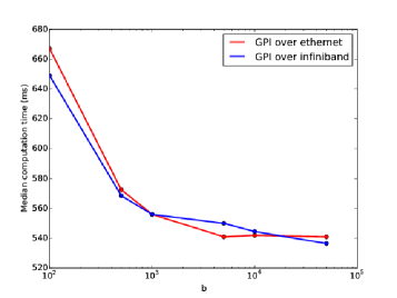
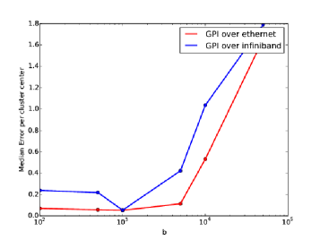
Figure 4: Comparing ASGD performance on Gigabit-Ethernet vs. Infiniband interconnections. LEFT: Median runtime of ASGD for altering communication frequencies $1\over b$. RIGHT: Median Error rates of ASGD Results on Synthetic data with $D=10,K=10$, which results in small messages ($50$ byte) shows hardly any difference between the performance of both connection types.

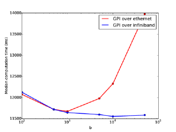
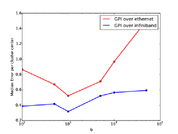
Figure 5: Same experiments as in figure 4, but with a lager problem ($D=100,K=100$: message size $5$kB) shows significant differences in performance. Notably, the Gigabit-Ethernet interconnect shows a local optimum for $b=1000$.

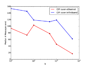
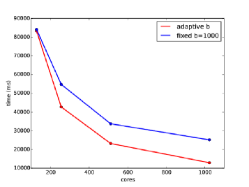
Figure 6: LEFT: Same experiments as in figure 5, showing the median number of “good” messages send. Again, the Gigabit-Ethernet interconnect shows a local optimum for $b=1000$. RIGHT: Evaluation of the scaling properties of ASGD on Gigabit-Ethernet. Comparing a fixed $b$ and our new adaptive $b$ algorithm.

Results.

Figure 4 shows that the performance of the ASGD algorithm for problems with small message sizes is hardly influenced by the network bandwidth. Gigabit-Ethernet and Infiniband implementations have approximately the same performance. This situation changes, when the message size in increased. Figure 5 shows that the performance is breaking down, as soon as the Gigabit-Ethernet connections reach their bandwidth limit.
Figure 6 shows that this effect can be softened by the usage of our adaptive message frequency algorithm, automatically selecting the current maximum frequency which will not exceed the available bandwidth.

5 Conclusions

The introduced load balancing algorithm simplifies the usage of the ASGD optimization algorithm in machine learning applications on HTC environments.

References

- [1] K. Bhaduri, K. Das, K. Liu, and H. Kargupta. Distributed data mining bibliography. In http://www.csee.umbc.edu/ hillol/DDMBIB/.
- [2] L. Bottou. Large-scale machine learning with stochastic gradient descent. In Proceedings of COMPSTAT’2010, pages 177–186. Springer, 2010.
- [3] L. Bottou and Y. Bengio. Convergence properties of the k-means algorithms. In Advances in Neural Information Processing Systems 7,[NIPS Conference, Denver, Colorado, USA, 1994], pages 585–592, 1994.
- [4] L. Bottou and O. Bousquet. The tradeoffs of large-scale learning. In Neural Information Processing Systems 20, pages 161–168. MIT Press, 2008.
- [5] C. Chu, S. K. Kim, Y.-A. Lin, Y. Yu, G. Bradski, A. Y. Ng, and K. Olukotun. Map-reduce for machine learning on multicore. Advances in neural information processing systems, 19:281, 2007.
- [6] D. Grünewald and C. Simmendinger. The gaspi api specification and its implementation gpi 2.0. In 7th International Conference on PGAS Programming Models, volume 243, 2013.
- [7] A. K. Jain. Data clustering: 50 years beyond k-means. Pattern recognition letters, 31(8):651–666, 2010.
- [8] J. Keuper and F.-J. Pfreundt. Asynchronous parallel stochastic gradient descent - a numeric core for scalable distributed machine learning algorithms. In arxiv.org/abs/1505.04956, 2015.
- [9] S. Lloyd. Least squares quantization in pcm. Information Theory, IEEE Transactions on, 28(2):129–137, 1982.
- [10] M. Meila. The uniqueness of a good optimum for k-means. In Proc. 23rd Internat. Conf. Machine Learning, pages 625–632, 2006.
- [11] B. Recht, C. Re, S. Wright, and F. Niu. Hogwild: A lock-free approach to parallelizing stochastic gradient descent. In Advances in Neural Information Processing Systems, pages 693–701, 2011.
- [12] D. Sculley. Web-scale k-means clustering. In Proceedings of the 19th international conference on World wide web, pages 1177–1178. ACM, 2010.
- [13] M. Zinkevich, M. Weimer, L. Li, and A. J. Smola. Parallelized stochastic gradient descent. In Advances in Neural Information Processing Systems, pages 2595–2603, 2010.