Stationary shapes of deformable particles moving at low Reynolds numbers

Abstract

Lecture Notes of the Summer School “Microswimmers – From Single Particle Motion to Collective Behaviour”, organised by the DFG Priority Programme SPP 1726 (Forschungszentrum Jülich, 2015).

I Introduction

The motion of deformable micron-sized objects though a viscous fluid represents an important problem with various applications, for example, for elastic microcapsules Barthès-Biesel (2011), red blood cells Fedosov et al. (2014); Freund (2014) or vesicles moving in capillaries, deforming in shear flow, or sedimenting under gravity Abreu et al. (2014); Huang et al. (2011). Another related system are droplets moving in a viscous fluid Clift et al. (1978); Stone (1994). Motion of these deformable objects can be caused by external body forces, as in sedimentation under gravity or in a centrifuge, dragging the object through a quiescent fluid, or, in the absence of driving forces, by putting the object into a hydrodynamic flow, for example, capillary flow. In the context of microswimmers, another possibility is self-propulsion of a soft microswimmer, for example, by fluid flows generated at its surface. On the micrometer scale, the hydrodynamic flows involved in the motion of these objects feature low Reynolds numbers unless the particle velocities become very high. Many elastic micron-sized objects, such as capsules, vesicles or red blood cells, are easily deformable because elasticity only stems from a thin elastic shell surrounding a liquid core. The analytical description and the simulation are challenging problems as the hydrodynamics of the fluid is coupled to the elastic deformation of the capsule or vesicle. It is important to recognise that this coupling is mutual: On the one hand, hydrodynamic forces deform a soft capsule, a vesicle, or a droplet. On the other hand, the deformed capsule, vesicle or droplet changes the boundary conditions for the fluid flow. As a result of this interplay, the soft object deforms and takes on characteristic shapes; eventually there are transitions between different shapes as a function of the driving force or flow velocity. Such shape changes might have important consequences for applications or biological function, for example, if we consider red blood cells or microcapsule containers moving in narrow capillaries. Shapes can also exhibit additional dynamic features such as tank-treading or tumbling, as it has been shown experimentally and theoretically for vesicles or elastic capsules in shear flows Barthès-Biesel (2011); Abreu et al. (2014). In the following, we investigate stationary shapes of elastic capsules sedimenting in an otherwise quiescent incompressible fluid, either by gravity or by the centrifugal force. Possible shapes and the nature of dynamic transitions between them are only poorly understood for sedimenting capsules. An elastic capsule is a closed elastic shell, i.e., a two-dimensional solid, which can support in-plane shear stresses and inhomogeneous stretching stresses with respect to their equilibrium configuration. This is different from a fluid vesicle, which is governed by bending elasticity only and is bounded by a two-dimensional fluid surface (lipid membrane) with vanishing shear modulus Seifert (1997). Whereas the rest shape of vesicles is determined by a few global parameters such as fixed area and spontaneous curvature Seifert (1997), elastic capsules can be produced with arbitrary rest shapes, in principle. We focus on elastic microcapsules with a spherical rest shape. We use this problem to introduce a method to calculate efficiently axisymmetric stationary capsules shapes, which iterates between a boundary integral method to solve the viscous flow problem for given capsule shape and capsule shape equations to calculate the capsule shape in a given fluid velocity field. The method does not capture the dynamic evolution of the capsule shape but converges to its stationary shape.

II Prologue – Cauchy momentum equation

The unifying concept of both the shape of an elastic capsule and the motion of a viscous fluid is continuum mechanics. The fundamental equation in point mechanics is Newton’s second law

$$\frac{\mathrm{d}\mathbf{P}}{\mathrm{d}t} =\mathbf{F}\text{,}$$ (1)

that is the change of the momentum $\mathbf{P}$ is given by the net force $\mathbf{F}$ acting on a mass point. In order to formulate the equivalent equation for a continuous medium, we consider a volume element $\mathrm{d}V$ with mass $\rho\mathrm{d}V$ moving with velocity $\mathbf{u}(\mathbf{r},t)$. We stress the fact that $\mathbf{u}$ is a field variable: there is a velocity for every point $\mathbf{r}$ in the total volume, $\Omega$, and every time $t$ considered. For the change of momentum of a specific volume element that moves in time, we have to track its motion and compute the total time derivative of $\mathbf{u}(\mathbf{r}(t),t)$ along the path of its motion Batchelor (2000), that is with $\partial_{t}\mathbf{r}(t)=\mathbf{u}$, which is called the material derivative

$$\frac{\mathrm{D}(\rho\mathbf{u})}{\mathrm{D}t}\equiv\frac{\partial(\rho\mathbf{u})}{\partial t}+\rho\mathbf{u}\cdot\nabla(\rho\mathbf{u})\text{.}$$ (2)

There can be two types of force acting on the volume element, interfacial forces $\mathbf{f}_{i}$ due to the interaction with neighbouring volume elements acting on the surface and body forces $\mathbf{b}$ acting on the volume, and we can adapt Newton’s law to

$$\int_{\Omega}\mathrm{d}V\,\frac{\mathrm{D}(\rho\mathbf{u})}{\mathrm{D}t}=\int_{\partial\Omega}\mathrm{d}A\mathbf{f}_{i}+\int_{\Omega}\mathrm{d}V\,\mathbf{b}=\int_{\Omega}\mathrm{d}V\,\left[\nabla\cdot\sigma+\mathbf{b}\right]\text{.}$$ (3)

We wrote $\mathbf{f}_{i}=\sigma\cdot\mathbf{n}$ with the surface normal $\mathbf{n}$, where we call $\sigma$ the stress tensor, and applied Stokes’ theorem in the last equality. Because it holds for arbitrary $\Omega$, the integrands are equal, which yields the Cauchy momentum equation

$$\frac{\mathrm{D}(\rho\mathbf{u})}{\mathrm{D}t}=\nabla\cdot\sigma+\mathbf{b}\text{.}$$ (4)

In the following, we consider this equation both for volume elements of fluid and for volume elements of the capsule membrane. For the fluid and for the capsule material there are different constitutive relations, which describe the relation between the stresses $\sigma$ in the medium and the deformation state or velocity field (stress-strain-relation). The left-hand side of this equation will be zero both for capsule and fluid, as we consider a stationary capsule shape ($\mathbf{u}=0$) and a stationary, incompressible (or solenoid, if you will) fluid flow at low Reynolds number. In this stationary case, we obtain stress-balance equations for the fluid and the capsule shape. Both equations are coupled: The fluid stresses enter the stress-balance for the capsule. Moreover, the fluid velocity field is required to be continuous at the boundary between capsule and fluid resulting in a no-slip boundary condition at the capsule surface.

III Equilibrium shape of a thin shell

For the parametrisation of the capsule shape, we directly exploit the axisymmetry by working in cylindrical coordinates. The axis of symmetry is called $z$, the distance to this axis $r$ and the polar angle $\phi$. The shell is given by the generatrix $(r(s),z(s))$ which is parametrised in arc-length $s$ (starting at the lower apex with $s=0$ and ending at the upper apex with $s=L$). The unit tangent vector $\mathbf{e}_{s}$ to the generatrix at $(r(s),z(s))$ defines an angle $\psi$ via $\mathbf{e}_{s}=(\cos\psi,\sin\psi)$, which can be used to quantify the orientation of a patch of the capsule relative to the axis of symmetry. The shape of a thin axisymmetric shell of thickness $H$ can be derived from non-linear shell theory Libai and Simmonds (1998); Pozrikidis (2003). A known reference shape $(r_{0}(s_{0}),z_{0}(s_{0}))$ (a subscript zero refers to a quantity of the reference shape; $s_{0}\in[0,L_{0}]$ is the arc length of the reference shape) is deformed by hydrodynamic forces exerted by the viscous flow. Each point $(r_{0}(s_{0}),z_{0}(s_{0}))$ is mapped onto a point $(r(s_{0}),z(s_{0}))$ in the deformed configuration, which induces meridional and circumferential stretches, $\lambda_{s}=ds/ds_{0}$ and $\lambda_{\phi}=r/r_{0}$, respectively. The arc length element $\mathrm{d}s$ of the deformed configuration is $\mathrm{d}s^{2}=(r^{\prime}(s_{0})^{2}+z^{\prime}(s_{0})^{2})\mathrm{d}s_{0}^{2}$. The shape of the deformed axisymmetric shell is given by the solution of a system of first-order differential equations, henceforth referred to as the shape equations. These describe stress-balance, i.e., the balance forces and torques or tensions and bending moments acting on a patch of the shell, as shown in Fig. 1. Using the notation of Refs. Knoche and Kierfeld (2011); Knoche et al. (2013) these can be written as

$$s^{\prime}(s_{0}) =\lambda_{s}$$ (5a)

$$r^{\prime}(s_{0}) =\lambda_{s}\cos{\psi}$$ (5b)

$$z^{\prime}(s_{0}) =\lambda_{s}\sin{\psi}$$ (5c)

$$\psi^{\prime}(s_{0}) =\lambda_{s}\kappa_{s}$$ (5d)

$$\tau^{\prime}_{s}(s_{0}) =\lambda_{s}\left(\frac{\tau_{\phi}-\tau_{s}}{r}\cos\psi+\kappa_{s}q+p_{s}\right)$$ (5e)

$$m^{\prime}_{s}(s_{0}) =\lambda_{s}\left(\frac{m_{\phi}-m_{s}}{r}\cos\psi-q+l\right)$$ (5f)

$$q^{\prime}(s_{0}) =\lambda_{s}\left(-\kappa_{s}\tau_{s}-\kappa_{\phi}\tau_{\phi}-\frac{q}{r}\cos\psi+p\right)\text{.}$$ (5g)

Figure 1: Sketch depicting the tensions and moments

The additional quantities appearing in these shape equations are defined as follows: The angle $\psi$ is the slope angle between the tangent plane to the deformed shape and the $r$-axis, $\kappa_{\phi}$ is the circumferential curvature, $\kappa_{s}$ the meridional curvature; $\tau_{s}$ and $\tau_{\phi}$ are the meridional and circumferential stresses, respectively; $m_{s}$ and $m_{\phi}$ are bending moments; $q$ is the transverse shear stress, $p$ the total normal pressure, $p_{s}$ the shear pressure, and $l$ the external stress couple. The first equation defines $\lambda_{s}$, the next three equations follow from geometry, and the last three ones express (tangential and normal) force and torque equilibrium. All quantities appearing on the right hand side of the shape equations have to be expressed in terms of the 7 quantities on the left hand side in order to close the equations.

The curvatures and circumferential strains are known from geometrical relations $\kappa_{\phi}=\frac{\sin\psi}{r}$, $\kappa_{s}=\frac{\mathrm{d}\psi}{\mathrm{d}s}$ and $\lambda_{\phi}=\frac{r}{r_{0}}$. The elastic tensions $\tau_{s}$ and $\tau_{\phi}$ and bending moments $m_{s}$ and $m_{\phi}$, which define the elastic stresses in the shell material are related to the strains and curvatures by the material-specific constitutive relations, which relate the stress tensor in a material to the strain tensor and involve the elastic constants of the material. Such constitutive relations often derive from an elastic energy functional, such that the stress tensor components are the first variation of the energy functional with respect to the corresponding strain tensor components Landau and Lifshitz (1986). We will derive the general relation between stress tensor and elastic tensions and bending moments of the shell in the following section.

Below, we will focus on Hookean capsules, where the constitutive relations derive from an elastic energy which is quadratic in stretching strains and bending strains. This leads to Libai and Simmonds (1998); Knoche et al. (2013)

$$\tau_{s} =\frac{Y_{\rm 2D}}{1-\nu_{\rm 2D}^{2}}\frac{1}{\lambda_{\phi}}\left[(\lambda_{s}-1)+\nu_{\rm 2D}(\lambda_{\phi}-1)\right]$$ (6)

$$m_{s} =E_{B}\frac{1}{\lambda_{\phi}}\left[(\lambda_{s}\kappa_{s}-\kappa_{s0})+\nu_{\rm 2D}(\lambda_{\phi}\kappa_{\phi}-\kappa_{\phi 0})\right]$$ (7)

where $Y_{\rm 2D}$ is the surface Young modulus (which, for isotropic shells, is related to the bulk Young modulus by $Y_{\rm 2D}=Y_{\rm 3D}H$), $\nu_{\rm 2D}$ is the surface Poisson ratio, and $E_{B}$ is the bending modulus of the shell ($E_{B}\propto Y_{\rm 2D}H^{2}$ for isotropic shells); $\kappa_{s0}$ and $\kappa_{\phi 0}$ are the curvatures of the reference shape. The constitutive relations for $\tau_{\phi}$ and $m_{\phi}$ are obtained by interchanging all indices $s$ and $\phi$.

The normal pressure

$$p =p_{0}+p_{n}+p_{\text{ext}},$$ (8)

the shear-pressure $p_{s}$, and the stress couple $l=p_{s}H/2$ are given externally by hydrodynamic and external forces. The static pressure $p_{0}$ is the pressure difference between the interior and exterior liquids. For the case of a capsule that is filled with an incompressible fluid its value is fixed by demanding a fixed enclosed volume.

The pressures $p_{n}$ and $p_{s}$ are the normal and tangential forces per area which are generated by the surrounding fluid. For the latter it would usually be more natural to give express stresses in terms of their radial and axial contributions. The vector

$$\mathbf{p}_{H} =p_{n}\mathbf{n}-p_{s}\mathbf{e}_{s},$$ (9)

where $\mathbf{n}$ and $\mathbf{e}_{s}$ are the normal and tangent unit vectors to the generatrix, $\mathbf{n}=-\cos\psi\mathbf{e}_{z}+\sin\psi\mathbf{e}_{r}$ and $\mathbf{e}_{s}=\sin\psi\mathbf{e}_{z}+\cos\psi\mathbf{e}_{r}$, equals the hydrodynamic surface force density vector

$$\mathbf{f}=f_{z}\mathbf{e}_{z}+f_{r}\mathbf{e}_{r}\text{,}$$ (10)

which will be calculated below. Re-decomposing $\mathbf{f}$ into its normal and tangential components $p_{n}$ and $p_{s}$ we find

$$p_{n} =f_{r}\sin\psi-f_{z}\cos\psi\quad\text{and}\quad p_{s}=-f_{r}\cos\psi-f_{z}\sin\psi\text{.}$$ (11)

III.1 Derivation of the shape equations

In the following, we present a compact derivation of the shape equations (5e), (5f) and (5g) describing force and torque balance. We refer the reader to the literature Libai and Simmonds (1998); Pozrikidis (2003); Knoche and Kierfeld (2011) for more elaborate derivations. From the Cauchy momentum equation we gather that the equilibrium is given by $\nabla\cdot\sigma=0$. We will not use Cartesian coordinates here, but curvilinear coordinates that are better suited to the capsule geometry. In the vicinity of the capsule we can parametrise space by the set of coordinates $n,s,\phi$ and

$$\mathbf{r}(n,s,\phi) =\left(\begin{array}[]{c}r(s)\cos\phi\\ r(s)\sin\phi\\ z(s)\end{array}\right)+n\left(\begin{array}[]{c}\sin\psi\cos\phi\\ \sin\psi\sin\phi\\ -\cos\psi\end{array}\right)$$ (18)

which corresponds to a local tripod of orthogonal vectors

$$\tilde{\mathbf{n}} =\left(\begin{array}[]{c}\sin\psi\cos\phi\\ \sin\psi\sin\phi\\ -\cos\psi\end{array}\right)\text{,}~{}~{}\tilde{\mathbf{s}}=(1+n\psi^{\prime})\left(\begin{array}[]{c}\cos\psi\cos\phi\\ \cos\psi\sin\phi\\ \sin\psi\end{array}\right)\,\text{and}~{}~{}\tilde{\bm{\phi}}=(r+n\sin\psi)\left(\begin{array}[]{c}\sin\phi\\ -\cos\phi\\ 0\end{array}\right).$$ (28)

Using index notation with $i,j,k\in{n,s,\phi}$, the tripod vectors can be written as $\tilde{\mathbf{i}}=\partial_{i}\mathbf{r}$. We want to derive equations for the elasticity of a thin shell, which we treat as an effectively two-dimensional surface. This is done by restricting stresses to in-plane stresses and integrating over the normal direction (the $n$-direction, $n\in[-H/2,H/2]$ with $H$ being the thickness). Thus, it is advantageous to define a projector $\mathsf{P}=\mathbbm{1}-\tilde{\mathbf{n}}\tilde{\mathbf{n}}$ that projects the stress onto the subspace of in-plane stresses. We then have to compute the tensor derivative occurring in the in-plane stress-balance equation $\nabla\cdot\mathsf{P}\sigma=0$ in these curvilinear coordinates. We can use the general result (to be read with Einstein summation convention)

$$(\nabla\cdot\mathsf{A})_{k} =\frac{\partial\mathsf{A}_{ik}}{\partial i}-\mathsf{A}_{jk}\Gamma^{j}_{ii}-\mathsf{A}_{ij}\Gamma^{j}_{ik}$$ (29)

with $i,j,k\in{n,s,\phi}$ and the Christoffel symbols of the second kind defined by $\frac{\partial\tilde{\mathbf{i}}}{\partial j}=\Gamma^{k}_{ij}\tilde{\mathbf{k}}$. The Christoffel symbols of the second kind are symmetric in the lower indices. For the non-vanishing symbols (at $n=0$, i.e. on the surface, where we want to evaluate the stress) we find

$$\Gamma^{s}_{ns}=\kappa_{s}\text{,}\,\Gamma^{\phi}_{n\phi}=\kappa_{\phi}\text{,}\,\Gamma^{n}_{ss}=-\kappa_{s}\text{,}\,\Gamma^{\phi}_{s\phi}=\frac{\cos\psi}{r}\text{,}\,\Gamma^{n}_{\phi\phi}=-r\sin\psi\,\text{ and }\,\Gamma^{s}_{\phi\phi}=-r\cos\psi\text{.}$$

Here, we made use of the geometrical relations $\psi^{\prime}=\kappa_{s}$ and $\sin\psi=r\kappa_{\phi}$. From the given axisymmetry, we infer the following form of the projected stress tensor

$$\mathsf{P}\sigma =\left(\begin{array}[]{ccc}0&0&0\\ \sigma_{sn}&\sigma_{ss}&0\\ 0&0&\sigma_{\phi\phi}\end{array}\right)$$ (33)

and computing the divergence (at $n=0$) finally yields (remember $\partial_{s}r=\cos\psi$)

$$\nabla\cdot\mathsf{P}\sigma =\left(\frac{1}{r}\frac{\partial(r\sigma_{sn})}{\partial s}-\kappa_{s}\sigma_{ss}-\sigma_{\phi\phi}\kappa_{\phi}\right)\tilde{\mathbf{n}}+\left(\frac{1}{r}\frac{\partial(r\sigma_{ss})}{\partial s}+\kappa_{s}\sigma_{sn}-\sigma_{\phi\phi}\frac{\cos\psi}{r}\right)\tilde{\mathbf{s}}\text{.}$$ (34)

If we integrate over the small thickness and introduce (the sign of $q$ might appear random and is such that the definition of $q$ agrees with the literature)

$$\int_{-H/2}^{H/2}\mathrm{d}n\,\sigma_{ss} =\tau_{s}\text{,}\quad\int_{-H/2}^{H/2}\mathrm{d}n\,\sigma_{\phi\phi}=\tau_{\phi}\quad\text{and}\quad\int_{-H/2}^{H/2}\mathrm{d}n\,\sigma_{sn}=-q\text{.}$$ (35)

The in-plane stress-balance $\nabla\cdot\mathsf{P}\sigma=0$ then establishes the shape equations (5e) and (5g).

The third equation (5f) is obtained from considering the acting torque. A shell of finite thickness is able to sustain finite interfacial bending moments $\mathbf{m}$, which, in terms of basic physics, means that there is an additional contribution to the torque balance. Arguing along the same lines as we did for the Cauchy momentum equation but starting from Newton’s second law for rotational motion,

$$\frac{\mathrm{d}L}{\mathrm{d}t} =\mathbf{M}\text{,}$$ (36)

yields (in equilibrium)

$$0 =\int_{\Omega}\mathrm{d}V(\mathbf{r}^{\prime}\times\mathbf{b})+\int_{\partial\Omega}\mathrm{d}A(\mathbf{r}^{\prime}\times\sigma\mathbf{n}_{A}+\mathbf{m})$$ (37)

where $\mathbf{r}^{\prime}$ is the difference vector to the centre of mass of the patch. Now we introduce the bending moment tensor (also couple stress tensor) $\mathsf{M}$ by $\mathbf{m}=\mathsf{M}\mathbf{n}_{A}$ ($\mathbf{n}_{A}$ is the three-dimensional normal to the surface $A$) and the auxiliary tensor $\mathsf{D}$ by $\mathsf{D}\cdot\mathbf{n}_{A}=\mathbf{r}^{\prime}\times\sigma\cdot\mathbf{n}_{A}$; after once again applying the divergence theorem we find, in absence of body forces, $\nabla\cdot\left(\mathsf{D}+\mathsf{M}\right)=0$. We are interested in the axisymmetric case $\mathbf{n}_{A}=\tilde{\mathbf{n}}$ and (after projection to in-plane stresses) see that $\sigma\tilde{\mathbf{n}}=\sigma_{sn}\tilde{\mathbf{s}}$. We consider a small patch such that we can write $\mathbf{r^{\prime}}=s\tilde{\mathbf{s}}+n\tilde{\mathbf{n}}+\phi\tilde{\mathbf{\phi}}$ and find after projection to in-plane-torques and using that the internal bending moments act along the directions of principal curvature, i.e.

$$\mathsf{P}\mathsf{M} =\left(\begin{array}[]{ccc}0&0&0\\ 0&M_{ss}&0\\ 0&0&M_{\phi\phi}\end{array}\right)\text{,}$$ (41)

for $n=0$

$$0 =\frac{1}{r}\frac{\partial rM_{ss}}{\partial s}+\sigma_{sn}-\frac{\cos\psi}{r}M_{\phi\phi}$$ (42)

which gives equation (5f) after renaming

$$\int_{-H/2}^{H/2}\mathrm{d}n\,M_{ss} =m_{s}\quad\text{and}\quad\int_{-H/2}^{H/2}\mathrm{d}n\,M_{\phi\phi}=m_{\phi}\text{.}$$ (43)

III.2 Solution of the shape equations.

The boundary conditions for a shape that is closed and has no kinks at its poles are

$$r(0)=r(L_{0})=\psi(0)=\pi-\psi(L_{0})=0,$$ (44)

and we can always choose $z(0)=0$. If hydrodynamic drag and gravitational pull cancel each other in a stationary state, there is no remaining point force at the poles needed to ensure equilibrium and, thus,

$$q(0) =q(L_{0})=0\text{.}$$ (45)

The shape equations have (removable) singularities at both poles; therefore, a numerical solution has to start at both poles requiring $12$ boundary conditions ($r,z,\psi,\tau,m,q$ at both poles) out of which we know $7$ (by eqs. (44) and (45) and $z(0)=0$). The $5$ remaining parameters can be determined by a shooting method requiring that the solutions starting at $s_{0}=0$ and $s_{0}=L_{0}$ have to match continuously in the middle, which gives $6$ matching conditions ($r,z,\psi,\tau,m,q$). This gives an over-determined non-linear set of equations which we solve iteratively using linearizations. However, as in the static case Knoche and Kierfeld (2011), the existence of a solution to the resulting system of linear equations (the matching conditions) is ensured by the existence of a first integral (see below) of the shape equation. In principle, this first integral could be used to cancel out the matching condition for one parameter (e.g. $q$), such that the system is not genuinely over-determined. We found the approach using an over-determined system to be better numerically tractable, where we ultimately used a multiple shooting method including several matching points between the poles.

Using these boundary conditions, it is straightforward to see that the shape equations do not allow for a solution whose shape is the reference shape, unless there are no external loads ($p_{s}=p=l=0$).

III.3 First Integral of the shape equations

We make the following Ansatz (cf. eqs. (17), (22) in Ref. Knoche and Kierfeld (2011)) for a first integral of the shape equations

$$U(s) =2\pi r\cos\psi q+2\pi r\sin\psi\tau_{s}+X=\text{const.}$$ (46)

We are also assuming that the pressure $p$ and the shear pressure $p_{s}$ can be written as functions of the arc length $s$ only. The calculation is rather straightforward, we differentiate and get

$$0 =U^{\prime}(s)$$

$$=2\pi\cos^{2}\psi q-2\pi r\sin\psi\kappa_{s}q+2\pi r\cos\psi(-\kappa_{s}\tau_{s}-\kappa_{\phi}\tau_{\phi}-\cos\psi\frac{q}{r}+p)+2\pi\cos\psi\sin\psi\tau_{s}$$

$$~{}+2\pi r\cos\psi\kappa_{s}\tau_{s}+2\pi r\sin\psi(\cos\psi\frac{\tau_{\phi}-\tau_{s}}{r}+\kappa_{s}q+p_{s})+X^{\prime}$$ (47)

$$=2\pi rp\cos\psi+2\pi rp_{s}\sin\psi+X^{\prime}=0.$$ (48)

In the second to last step most terms cancel each other out. Thus, we arrive at an ordinary differential equation for $X$, which we can integrate to find

$$X(s) =-2\pi\int_{0}^{s}\mathrm{d}x\,r(p\cos\psi+p_{s}\sin\psi).$$ (49)

Inspecting the behaviour at $s=0$ we deduce $U(s)=U(0)=0$, which implies $U(L)=0$ and, according to (46), $X(L)=0$. The physical interpretation of $X(L)=0$ in (49) is that the capsule has to be in global force balance. By symmetry there can be no net force in radial direction, but the external forces can lead to net force in axial direction. The quantity $X$ contains the contribution to the net force in $z$-direction and thus a shape with the desired features (namely $q=0$ at the apexes) must have $X(L)=0$ and, thus, be in global force balance.

IV Low Reynolds-number Hydrodynamics

We want to calculate the flow field of a viscous incompressible fluid around an axisymmetric capsule of given fixed shape at low Reynolds numbers. We chose to separate the problems, which allows us to state that for the calculation of the flow field the deformability of the capsule is not relevant, and the capsule can be viewed as a general immersed body of revolution $\mathfrak{B}$. For the calculation of the capsule shape, which is addressed in the following section, and for the determination of its sedimenting velocity, we only need to calculate the surface forces onto the capsule which are generated by the fluid flow.

IV.1 Stokes equation

We start with the fundamental notion that the mass of the fluid should be conserved under its flow $\mathbf{u}$ giving rise to the continuity equation

$$\frac{\partial\rho}{\partial t} =-\nabla\cdot(\rho\mathbf{u})$$ (50)

with $\rho$ being the local mass density. Furthermore, we only consider incompressible fluids, thus, the density of a fluid volume element cannot change under its motion due to the flow or

$$0=\frac{D\rho}{Dt} =\frac{\partial\rho}{\partial t}+\mathbf{u}\cdot\nabla\rho\text{.}$$ (51)

We combine these two equations and find with some help from vector calculus

$$\nabla\cdot\mathbf{u} =0\text{,}$$ (52)

which is commonly referred to as the continuity equation for an incompressible flow. Using this equation in the Cauchy momentum equation, eq. (4), for a stationary flow with $\partial_{t}\mathbf{u}=0$ gives

$$\rho\mathbf{u}\cdot\nabla\mathbf{u} =\nabla\cdot\sigma\text{.}$$ (53)

For further progress, we need the constitutive relation for the liquid. Demanding Galilean invariance of $\sigma$, we see that $\sigma$ can only depend on spatial derivatives of the velocity and from conservation of angular momentum we know that $\sigma$ is symmetric. Based on experimental evidence we further demand that there are no shear stresses in a quiescent fluid, that $\sigma$ is isotropic and that stresses grow linear with the velocity, which allows us to write

$$\sigma =-p\mathbbm{1}+\mu\left(\nabla\mathbf{u}+(\nabla\mathbf{u})^{T}\right)\text{.}$$ (54)

or, in Cartesian coordinates, $\sigma_{ij}=-p\delta_{ij}+2\mu e_{ij}\text{,}$ with the pressure $p$, the viscosity $\mu$ and the rate of deformation (or rate of strain) tensor for the flow velocity $\mathbf{u}$

$$e_{ij} =\frac{1}{2}\left(\frac{\partial u_{i}}{\partial x_{j}}+\frac{\partial u_{j}}{\partial x_{i}}\right)\text{.}$$ (55)

A liquid for which our assumptions hold is called a Newtonian fluid. The constitutive relation together with eq. (53) (stationary Cauchy momentum equation for an incompressible fluid) give rise to the (stationary) Navier-Stokes equation. Rescaling velocities, lengths and stresses by their respective typical scales $u$, $R$, $\mu v/L$ (as inferred from the constitutive relation) in eq. (53) we obtain

$$\mathrm{Re}\,\bar{\mathbf{u}}\cdot\bar{\nabla}\bar{\mathbf{u}} =\bar{\nabla}\cdot\bar{\sigma}$$ (56)

for the corresponding dimensionless quantities $\bar{\mathbf{u}}$ and $\bar{\sigma}$ with the Reynolds number

$$\mathrm{Re} =\frac{\rho uL}{\mu}\text{.}$$ (57)

We can neglect the so-called advective term on the left hand-side of our equation of motion, if the Reynolds number is sufficiently low, that is for small, slowly moving particles in a medium of high viscosity. All in all, in the limit of small Reynolds numbers in a stationary fluid in the absence of external body forces, the stress tensor $\sigma$ is given by the stationary Stokes equation Happel and Brenner (1983)

$$\nabla\cdot\sigma =0\text{.}$$ (58)

IV.2 Lorentz’ reciprocal theorem

As a preliminary for the following, we derive a relation between two solutions of the Stokes equation, commonly known as Lorentz’ reciprocal theorem. Suppose we have two velocity fields $\tilde{\mathbf{u}}$, $\widehat{\mathbf{u}}$ with corresponding stress tensors $\tilde{\sigma}$, $\widehat{\sigma}$ both of which solve the Stokes equation (58) with the constitutive relation (54). Now, for reasons that will become apparent instantly, we look at the following rather odd expression

$$\tilde{\mathbf{u}}\cdot\left(\nabla\cdot\widehat{\sigma}\right) =\nabla\cdot\left(\tilde{\mathbf{u}}\widehat{\sigma}\right)-\left(\widehat{\sigma}\nabla\right)\tilde{\mathbf{u}}=\frac{\partial}{\partial x_{j}}\left(\tilde{u}_{i}\widehat{\sigma}_{ij}\right)-\mu\left(\frac{\partial\widehat{u}_{i}}{\partial x_{j}}+\frac{\partial\widehat{u}_{j}}{\partial x_{i}}\right)\frac{\partial\tilde{u}_{i}}{\partial x_{j}}\text{.}$$ (59)

where we inserted (54) and exploited that the pressure term vanishes due to the continuity equation. Subtracting (59) from its counterpart with tildes and hats interchanged we find that the terms involving the viscosity cancel out yielding

$$\widehat{\mathbf{u}}\cdot\left(\nabla\cdot\tilde{\sigma}\right)-\tilde{\mathbf{u}}\cdot\left(\nabla\cdot\widehat{\sigma}\right) =\nabla\cdot\left(\widehat{\mathbf{u}}\tilde{\sigma}\right)-\nabla\cdot\left(\tilde{\mathbf{u}}\widehat{\sigma}\right)\text{.}$$ (60)

Given that we assumed $\tilde{\sigma}$,$\widehat{\sigma}$ being solutions of eq. (58) we know that the left-hand side of the last equation is zero and we find the reciprocal identity

$$0 =\nabla\cdot\left(\widehat{\mathbf{u}}\tilde{\sigma}-\tilde{\mathbf{u}}\widehat{\sigma}\right)\text{.}$$ (61)

IV.3 Solution of the Stokes equation (in an axisymmetric domain)

In the rest frame of the sedimenting axisymmetric capsule and with a “no-slip” condition at the capsule surface $\partial\mathfrak{B}$, we are looking for axisymmetric solutions that have a given flow velocity $\mathbf{u}^{\infty}$ at infinity and vanishing velocity on the capsule boundary. In the lab frame, $-\mathbf{u}^{\infty}$ is the sedimenting velocity of the capsule in the stationary state. Therefore, $\mathbf{u}^{\infty}$ has to be determined by balancing the total gravitational pulling force and the total hydrodynamic drag force on the capsule. For the calculation of the flow field the deformability of the capsule is not relevant and the capsule can be viewed as a general immersed body of revolution $\mathfrak{B}$. For the calculation of the total hydrodynamic drag force and for the calculation of the capsule shape we need the surface force field $\mathbf{f}=\sigma\cdot\mathbf{n}$ generated by the flow, where $\mathbf{n}$ is the local surface normal. This is the only property of the fluid flow entering the shape equations for the capsule and the equation for the sedimenting velocity $|\mathbf{u}^{\infty}|$. In the lab frame we are looking for solutions with vanishing pressure and velocity at infinity. The Green’s function for these boundary condition is the well-known Stokeslet (also called Oseen-Burgers tensor), that is the fluid velocity $\mathbf{u}$ at $\mathbf{y}$ due to a point-force $-\mathbf{F}_{p}$ at $\mathbf{x}$

$$\mathbf{u}(\mathbf{y}) =-\frac{1}{8\pi\mu}\mathsf{G}(\mathbf{y}-\mathbf{x})\cdot\mathbf{F}_{p}$$ (64)

with the Stokeslet $\mathsf{G}$ whose elements are in Cartesian coordinates ($x=\lvert\mathbf{x}\rvert$)

$$\mathsf{G}_{ij}(\mathbf{x}) =\frac{\delta_{ij}}{x}+\frac{x_{i}x_{j}}{x^{3}}\text{.}$$ (65)

The corresponding stress tensor is given by

$$\sigma_{ij}(\mathbf{y}) =\frac{1}{8\pi}\mathsf{T}(\mathbf{y}-\mathbf{x})\cdot\mathbf{F}_{p}$$ (66)

with the Stresslet $\mathsf{T}$ whose Cartesian elements are

$$\mathsf{T}_{ijk}(\mathbf{x}) =-6\frac{x_{i}x_{j}x_{k}}{x^{5}}\text{.}$$ (67)

From the reciprocal theorem (61) we deduce (as $\mathbf{F}_{p}$ is a constant) that any solution of the Stokes equation has to satisfy

$$0 =\frac{\partial}{\partial y_{k}}\left(\mathsf{G}_{ij}(\mathbf{y}-\mathbf{x})\sigma_{ik}(\mathbf{y})-\mu u_{i}(\mathbf{y})\mathsf{T}_{ijk}(\mathbf{y}-\mathbf{x})\right)$$ (68)

or, after integrating over a volume with surface $\partial V$ by virtue of Stokes theorem,

$$\iint_{\partial V}\!\mathrm{d}\mathbf{A}\,\left(\mathsf{G}_{ij}(\mathbf{y}-\mathbf{x})\sigma_{ik}(\mathbf{y})-\mu u_{i}(\mathbf{y})\mathsf{T}_{ijk}(\mathbf{y}-\mathbf{x})\right) =0$$ (69)

For this equation to be valid the volume $V$ must not contain the singularity at $\mathbf{x}$. A straightforward way to ensure this is to consider the volume enclosed by $\partial\mathfrak{B}$ and $\partial B_{\varepsilon}(\mathbf{x})$, where the latter is the ball of infinitesimal size $\varepsilon$ around $\mathbf{x}$. Separating the surface integral this leads to

$$\iint_{\partial\mathfrak{B}}\!\mathrm{d}\mathbf{A}\,\left(\mathsf{G}_{ij}(\mathbf{y}-\mathbf{x})\sigma_{ik}(\mathbf{y})-\mu u_{i}(\mathbf{y})\mathsf{T}_{ijk}(\mathbf{y}-\mathbf{x})\right)$$ (70)

$$=-\iint_{\partial B_{\varepsilon}(\mathbf{x})}\!\mathrm{d}\mathbf{A}\,\left(\mathsf{G}_{ij}(\mathbf{y}-\mathbf{x})\sigma_{ik}(\mathbf{y})-\mu u_{i}(\mathbf{y})\mathsf{T}_{ijk}(\mathbf{y}-\mathbf{x})\right)$$ (71)

In the limit $\varepsilon\rightarrow 0$ we can simplify the right-hand side with $\mathbf{z}=\mathbf{y}-\mathbf{x}$ and $\mathrm{d}\mathbf{A}=\mathbf{n}\mathrm{d}A=\varepsilon^{-1}\mathbf{z}\varepsilon^{2}\mathrm{d}\Omega$ ($\Omega$ being the solid angle)

$$\iint_{\partial B_{\varepsilon}(\mathbf{y})}\!\!\!\!\!\!\!\!\!\!\mathrm{d}\mathbf{A}\,\left(\mathsf{G}_{ij}(\mathbf{y}-\mathbf{x})\sigma_{ik}(\mathbf{x})-\mu u_{i}(\mathbf{y})\mathsf{T}_{ijk}(\mathbf{y}-\mathbf{x})\right)+\mathcal{O}(\varepsilon)$$ (72)

$$=\iint_{\partial B_{\varepsilon}(\mathbf{y})}\!\!\!\!\!\!\!\!\!\!\mathrm{d}\Omega\,z_{k}\left(\left[\delta_{ij}+\frac{z_{i}z_{j}}{\varepsilon^{2}}\right]\sigma_{ik}(\mathbf{x})+\mu u_{i}(\mathbf{x})\left[6\frac{z_{i}z_{j}z_{k}}{\varepsilon^{4}}\right]\right)=\iint_{\partial B_{\varepsilon}(\mathbf{y})}\!\!\!\!\!\!\!\!\!\!\mathrm{d}\Omega\,z_{k}\left(\mu u_{i}(\mathbf{x})\left[6\frac{z_{i}z_{j}z_{k}}{\varepsilon^{4}}\right]\right)$$ (73)

$$=\frac{6\mu u_{i}(\mathbf{x})}{\varepsilon^{2}}\iint_{\partial B_{\varepsilon}(\mathbf{y})}\!\!\!\!\!\!\!\!\!\!\mathrm{d}\Omega\,\left(z_{i}z_{j}\right)=\frac{6\mu u_{i}(\mathbf{x})}{\varepsilon^{2}}2\pi\varepsilon^{2}\delta_{ij}\int_{-1}^{1}\!\mathrm{d}(\cos\theta)\cos^{2}\theta=8\pi\mu u_{j}(\mathbf{x})$$ (74)

and thus gather the boundary integral formula, which we express as a function of the acting surface forces $\mathbf{f}=\sigma\cdot\mathbf{n}$ including a constant velocity accounting for the centre of mass motion of the capsule

$$u_{j}(\mathbf{x})-u_{j}^{\infty}(\mathbf{x}) =-\frac{1}{8\pi\mu}\iint_{\partial\mathfrak{B}}\!\mathrm{d}A\,\mathsf{G}_{ij}(\mathbf{y}-\mathbf{x})f_{i}(\mathbf{y})+\iint_{\partial\mathfrak{B}}\!\mathrm{d}\mathbf{A}\,\frac{1}{8\pi}u_{i}(\mathbf{y})\mathsf{T}_{ijk}(\mathbf{y}-\mathbf{x})\text{.}$$ (75)

The physical interpretation of this equation is that the flow field is, on the one hand, due to point forces (first term, also called the single layer potential) and, on the other hand, due to point sources and force dipoles (second term, also called the double layer potential). The representation of a Stokes flow in terms of a single-layer potential is possible, if there is no net flow through the surface of the capsule Pozrikidis (1992), $\int\!\mathrm{d}A\,(\mathbf{u}-\mathbf{u}^{\infty})\cdot\mathbf{n}=0\text{,}$ which is the case for the no-slip boundary condition we are interested in.

In the case of axisymmetry we can integrate over the polar angle and find the general solution of the Stokes equation for an axisymmetric point force distribution,

$$u_{\alpha}(\mathbf{x})-u_{\alpha}^{\infty}(\mathbf{x}) =-\frac{1}{8\pi\mu}\int_{C}\mathrm{d}s(\mathbf{y})\mathsf{M}_{\alpha\beta}(\mathbf{y},\mathbf{x})f_{\beta}(\mathbf{y})\text{.}$$ (76)

Here, Greek indices denote the components in cylindrical coordinates, i.e., $\alpha,\beta=r,z$ ($u_{\phi}=f_{\phi}=0$ for symmetry reasons). The integration in (76) runs along the path $C$ given by the generatrix, i.e., the cross section of the boundary $\partial\mathfrak{B}$, with arc length $s(\mathbf{x})$.

According to the “no-slip” condition this results in the equation

$$u_{\alpha}^{\infty} =\frac{1}{8\pi\mu}\int_{C}\mathrm{d}s(\mathbf{y})\mathsf{M}_{\alpha\beta}(\mathbf{y},\mathbf{x})f_{\beta}(\mathbf{y}) (\text{for}~{}\mathbf{x}\in\partial\mathfrak{B})\text{.}$$ (77)

To numerically solve the integral equation for the surface force $f(\mathbf{x}_{i})$ at a given set of points $\{\mathbf{x}_{i}\}$ ($i=1,\ldots,N$) one can employ a collocation method, the most simple case of which is to choose a discretised representation of the function $f_{\beta}(\mathbf{x})$ and approximate the integral in (77) by the rectangle method leading to a system of linear equations. We note that there are (integrable) logarithmic singularities in the diagonal components of $\mathsf{M}$ which have to be taken care of.

We can restrict our computations to the bare minimum, i.e., the surface forces needed for the calculation of the capsule shape but, thereby, have all necessary information to reconstruct the whole velocity field in the surrounding liquid. The possibility to limit the computation to the needed surface forces is one advantage of this approach to the solution of the Stokes equation in comparison to other approaches that rely on the velocities or the stream function in the whole domain Happel and Brenner (1983); Langtangen et al. (2002).

We assumed a “no-slip”-condition, that is the velocity directly at the surface of the immersed body vanishes in its resting frame. This is easily extended to the case of a non-vanishing tangential slip velocity is possible, however, to extend this boundary integral approach to incorporate a prescribed velocity field on the surface in the resting frame of the capsule Pozrikidis (1992). This will allow us to generalise the approach to model active swimmers Lauga and Powers (2009); Degen (2014) whose active locomotion can be captured by means of an effective flow field which is called the squirmer model Lighthill (1952); Blake (1971).

V Iterative solution of shape, flow and sedimenting velocity

We find a joint solution to the shape equations and the Stokes equation by solving them separately and iteratively, as illustrated in the scheme in Fig. 2, to converge to the desired solution: We assume a fixed axisymmetric shape and calculate the resulting hydrodynamic forces on the capsule for this shape. Then, we use the resulting hydrodynamic surface force density to calculate a new deformed shape. Using this new shape we re-calculate the hydrodynamic surface forces and so on. We iterate until a fixed point is reached. At the fixed point, our approach is self-consistent, i.e., the capsule shape from which hydrodynamic surface forces are calculated is identical to the capsule shape that is obtained by integration of the shape equation under the influence of exactly these hydrodynamic surface forces.

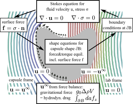
Figure 2: Iterative scheme for the solution to the problem of elastic capsules in Stokes flow allowing for the separation of the joint problem into two simpler static problems. Details of the iterative scheme are given in the main text.

For each capsule shape during the iteration, we can determine its sedimenting velocity $u=|\mathbf{u}^{\infty}|$ by requiring that the total hydrodynamic drag force equals the total driving force. Because the Stokes equation is linear in the velocity, the force equality is achieved by just rescaling the resulting surface drag forces accordingly via changing the velocity parameter $u$. The velocity therefore plays a similar role as a Lagrange multiplier for global force balance. In this way, the global force balance can be treated the same way as other possible constraints like a fixed volume. Numerically, it is impossible to ensure the exact equality of the drag and the drive forces, that is $X(L)\equiv 0$ (see eq. (49)). Demanding a very small residual force difference makes it difficult to find an adequate velocity, a too large force difference makes it impossible to find a solution with small errors at the matching points.

The iteration starts with a given (arbitrary) stress, e.g., one corresponding to the flow around the reference shape. For the resulting initial capsule shape, the Stokes flow is computed and the resulting stress is then used to start the iteration. If, during the iteration, the new and old stress differ strongly it might be difficult to find the new shooting parameters for the capsule shape and the right sedimenting velocity starting at their old values. To overcome this technical problem, one can use a convex combination $\sigma=\alpha\sigma_{\text{new}}+(1-\alpha)\sigma_{\text{old}}$ of the two stresses and slowly increase the contribution $\alpha$ of the new stress until it reaches unity. The resulting capsule shape for $\alpha=1$ is used to continue the iteration. The iteration continues until the change within one iteration cycle is sufficiently small. If there are multiple stationary solutions at a given gravitational strength the iterative procedure will obviously only find one. Therefore one has to use continuation of solutions to other parameters (different driving strength or bending modulus) and possibly multiple initial flows to get closer to the full set of solutions.

VI Application: Sedimenting Hookean capsules

As an application of the outlined method that illustrates the interplay of elasticity and low Reynolds-number hydrodynamics we consider the sedimentation of Hookean capsules. Sedimentation refers to the motion under the influence of gravity. However, an effective (and several orders of magnitude stronger) homogeneous body force can be created within a centrifuge. Thus, on a more general level we consider an external stress field of the form $p_{\text{ext}}=-g_{0}\Delta\rho z$. Here, $g_{0}$ is the gravitational acceleration and $\Delta\rho=\rho_{\rm in}-\rho_{\rm out}$ the density difference between the fluids inside and outside the capsule. Note that we measure the gravitational hydrostatic pressure $-g_{0}\Delta\rho z$ relative to the lower apex, for which we chose $z(0)=0$. We consider a capsule filled with an incompressible liquid and we therefore determine the static pressure imposing a volume constraint.

Non-dimensionalising this system using the capsule’s equilibrium radius $R_{0}$ and its elastic modulus $Y_{\rm 2D}$, the remaining free parameter are the strength of the gravitational pull (the Bond number ${\mathrm{B}o}\equiv{g_{0}\Delta\rho R_{0}^{2}}/{Y_{\rm 2D}}$) and the bending energy relative to the stretching energy (the inverse Föppl-von-Kármán number $1/\gamma_{\rm FvK}\equiv{E_{B}}/{Y_{\rm 2D}R_{0}^{2}}$).

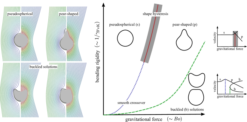
Figure 3: Schematic shape diagram of a sedimenting elastic capsule. The free parameters of the system are dimensionless bending rigidity and gravitational pull. We find four stable shapes, which are shown on the left together with the corresponding fluid streamlines (left: capsule frame, right: lab frame) and surface forces. The shaded area in the shape diagram in the middle indicates the area of coexistence of the pseudospherical and pearshaped solution branches, the blue dotted line is a crossover line. Along the green dashed line the two buckled shapes occur in a bifurcation. On the right we show schematics of typical force-velocity relations (depicting the ratio of the velocity of the capsule and the velocity of a rigid sphere of same volume as a function of the pull) for the two cases of low bending rigidities (no shape hysteresis with the additional branch of buckled solutions) and high bending rigidities (with shape hysteresis).

A schematic diagram of the stationary shapes that are found in this two-dimensional control parameter space is shown in Fig. 3. From Stokes’ solution for the flow around a sphere we see that the acting surface forces are $\sigma\cdot\mathbf{n}=\nicefrac{{3}}{{2R}}\,\mu u\mathbf{e}_{z}$. Thus, the viscous drag tends to stretch the capsule. Additionally the hydrostatic (gravitational) pressure effectively acts extensionally on the lower apex and compressional on the upper apex. This leads to a deformation towards pear shapes. For high bending rigidities the indentation of the flanks of the conical extension is suppressed by bending moments, leading to direct transition including shape hysteresis.

As in the static problem, the capsule can release stretching stress through buckling at sufficiently high external stress. However, in this problem these buckled solutions are coexistent with the pseudospherical/pear-shaped solutions.

VII Conclusion and Outlook

We showed that the joint problem of an elastic capsule’s motion in a viscous liquid at low Reynolds numbers can be reduced to iteratively solving two essentially static sub-problems, the elastic shape problem for fixed hydrodynamic forces and the stationary hydrodynamic Stokes flow problem for fixed boundary conditions from the capsule shape, if one is only interested in the stationary solution. We derived the relevant equations of motion and showed how to solve each the shape of an elastic capsule under a static external hydrodynamic stress and the flow field of a viscous liquid at low Reynolds number around a rigid (axisymmetric) body. We then combined these two sub-problem solutions and closed the problem by demanding stationarity under iteration.

Using this iterative method, we are able to resolve coexisting branches of stationary solutions in the problem of “passively” sedimenting elastic capsules. The method can also be adapted to “actively” swimming deformable objects. The most direct adaptation is possible for a deformable squirmer, where an elastic capsule with spherical rest shape generates a finite tangent slip velocity. This will change the boundary conditions of the viscous flow at the capsule surface from a no-slip boundary to a given tangential slip velocity (in the capsule frame). It is also conceivable to treat even more complex problems, such as a diffusiophoretic deformable swimmer, where one eventually has to include the solution of an appropriate diffusion equation as a third coupled sub-problem into the iterative procedure.

References

- Barthès-Biesel (2011) D. Barthès-Biesel, Curr. Opin. Colloid Interface Sci. 16, 3 (2011).
- Fedosov et al. (2014) D. A. Fedosov, H. Noguchi, and G. Gompper, Biomech. Model. Mechanobiol. 13, 239 (2014).
- Freund (2014) J. B. Freund, Annu. Rev. Fluid Mech. 46, 67 (2014).
- Abreu et al. (2014) D. Abreu, M. Levant, V. Steinberg, and U. Seifert, Adv. Colloid Interface Sci. 208, 129 (2014).
- Huang et al. (2011) Z. Huang, M. Abkarian, and A. Viallat, New J. Phys. 13, 035026 (2011).
- Clift et al. (1978) R. Clift, J. Grace, and M. Weber, Bubbles, Drops, and Particles (Academic Press, 1978).
- Stone (1994) H. A. Stone, Annu. Rev. Fluid Mech. 26, 65 (1994).
- Seifert (1997) U. Seifert, Adv. Phys. 46, 13 (1997).
- Batchelor (2000) G. K. Batchelor, An introduction to fluid dynamics (Cambridge university press, 2000).
- Libai and Simmonds (1998) A. Libai and J. Simmonds, The nonlinear theory of elastic shells (Cambridge University Press, Cambridge, 1998).
- Pozrikidis (2003) C. Pozrikidis, Modeling and simulation of capsules and biological cells (CRC Press, 2003).
- Knoche et al. (2013) S. Knoche, D. Vella, E. Aumaitre, P. Degen, H. Rehage, P. Cicuta, and J. Kierfeld, Langmuir 29, 12463 (2013).
- Knoche and Kierfeld (2011) S. Knoche and J. Kierfeld, Phys. Rev. E 84, 046608 (2011).
- Landau and Lifshitz (1986) L. Landau and E. Lifshitz, Theory of Elasticity, Vol. 7 (Pergamon, New York, 1986).
- Note (1) The fluid inside the capsule is assumed to be at rest.
- Note (2) The subscript indicates that this only incorporates the hydrodynamic contributions. We do not consider cases with a static shear-pressure but, as is apparent from eq. (8), there are static contributions to the normal pressure.
- Note (3) External forces are easily added and actually necessary for the existence of non-trivial solutions.
- Note (4) is a three-dimensional normal vector of the axisymmetric surface, whereas is a two-dimensional normal vector to the generatrix .
- Note (5) In the presence of gravity there is no translational symmetry along the axial direction, but shifting the capsule as a whole just adds a constant to the hydrostatic pressure which is absorbed into the static pressure .
- Note (6) We omit the external force as they do not change any of the following in a non-trivial manner.
- Note (7) This is sometimes referred to as Cauchy’s second law of motion (the first one being the momentum equation).
- Happel and Brenner (1983) J. Happel and H. Brenner, Low Reynolds number hydrodynamics: with special applications to particulate media, Vol. 1 (Springer, 1983).
- Note (8) This is an application of Green’s second identity of vector calculus.
-
Note (9)
We are looking for solutions of the Stokes equation with an
external point force,
Taking the divergence and using we obtain . This equation is solved (analogously to electrostatics) by(78)
Using this in the Stokes equation with point force, one obtains , where is the solution of , i.e., . This leads to the Stokeslet and Stresslet.(79) - Pozrikidis (1992) C. Pozrikidis, Boundary integral and singularity methods for linearized viscous flow (Cambridge University Press, 1992).
- Note (10) The elements of the matrix kernel can be expressed in terms of elliptic integrals, see for example Ref. Pozrikidis (1992).
- Langtangen et al. (2002) H. P. Langtangen, K.-A. Mardal, and R. Winther, Adv. Water Resour. 25, 1125 (2002).
- Note (11) A normal velocity on the surface in the capsule’s resting frame would conflict with its impenetrability and could also lead to a net flux of fluid through the capsule, which we cannot incorporate using only the single-layer potential.
- Lauga and Powers (2009) E. Lauga and T. R. Powers, Rep. Prog. Phys. 72, 096601 (2009).
- Degen (2014) P. Degen, Curr. Opin. Colloid Interface Sci. 19, 611 (2014).
- Lighthill (1952) M. Lighthill, Comm. Pure Appl. Math. 5, 109 (1952).
- Blake (1971) J. Blake, J. Fluid Mech. 46, 199 (1971).