Ferromagnetic resonance of magnetostatically-coupled shifted chains of nanoparticles in an oblique magnetic field

Abstract

We investigate the ferromagnetic resonance characteristics of a magnetic dimer composed of two shifted parallel chains of iron nanoparticles coupled by dipolar interactions. The latter are treated beyond the point-dipole approximation taking into account the finite size and arbitrary shape of the nano-elements and arbitrary separation. The resonance frequency is calculated as a function of the amplitude of the applied magnetic field and the resonance field is computed as a function of the direction of the applied field, varied both in the plane of the two chains and perpendicular to it. We highlight a critical value of the magnetic field which marks a state transition that should be important in magnetic recording media.

I introduction

Organized assemblies of nearly monodisperse nanoparticles are a recent achievement in materials science which is a result of a long-term endeavor of many research groups around the world (S. Sun, 2000; Lisiecki et al., 2003; P. Tartaj, P. Morales, S. Veintemillas-Verdaguer,T. Gonzalez-Carreño, and C. Serna, 2003). One of the main initial objectives for working towards this goal was to minimize the effects of volume and anisotropy distributions which make it more difficult, if not impossible, to access the intrinsic effects of magnetic nanoparticles. In parallel with this progress in fabrication and synthesis, several measuring techniques have benefited from considerable improvements with regards to time and spatial resolution. Some of the standard techniques, such as ferromagnetic resonance (FMR) (Vonsovskii, 1966; A.G. Gurevich and G.A. Melkov, 1996), stage a successful come-back (Duerr et al., 2011; Lee et al., 2011; Ding et al., 2012). The latter is a very efficient technique for characterizing assemblies of magnetic nanoparticles (Toulemon et al., 2016).

Accordingly, in this work we investigate the FMR characteristics of a monolayer of chains of (almost) monodisperse Fe nanoparticles of $D=20\ {\rm nm}$ in diameter. Within each chain, the particles are closely packed and touch each other, while the (nearly) parallel chains are a certain distance from each other, and may be shifted with respect to each other along their (major) axes. We investigate the effects of the inter-chain shift and separation on the FMR frequency and resonance field. These two parameters greatly affect the dipolar interactions (DI) between the chains, in addition to the size and shape of the chains. This aspect has been recently mentioned by Varón et al.(Varòn et al., 2013) in a study of the dipolar magnetism in ordered and disordered low-dimensional nanoparticle assemblies. In particular, these authors show that the DI are no longer negligible in such systems with respect to the usual prevalence of the exchange coupling in classical materials. In order to account for the effects of all these parameters, we shall consider here the more general formalism of DI (M. Beleggia S. Tandon, Y. Zhu, and M. De Graef, 2004; M. Beleggia, S. Tandon, Y. Zhu, and M. De Graef, 2004; A. F. Franco, J. L. Déjardin, and H. Kachkachi, 2014) between finite-size magnetic elements of cylindrical shape. From the applied physics standpoint, this investigation is of interest in the context of magnetic recording. Indeed, researchers have realized since the synthesis of FePt nanorods (Wang et al., 2013), that 1D nano-elements have a major advantage compared to more conventional nanoparticle assemblies. While spherical nanoparticles have magnetic moments that are difficult to texture, nanochains are usually aligned with one another due to geometric constraints (Toulemon, 2013; Toulemon et al., 2016). In addition, since a nanochain usually exhibits a magnetic anisotropy with an easy axis along the chain, these 1D nano-elements turn out to be quite promising to form bits with a well-defined orientation, owing to a strong magnetic signal and a large packing density. In this context, we compute the resonance frequency for both the binding and anti-binding modes and the resonance field as a function of the orientation of the applied external magnetic field. This is also motivated by the fact that the difference in frequency between the two modes in a pair of ($200$ nm) disks can now be measured with the help of Magnetic Resonance Force Microscopy as a function of the nanodisks separation (B. Pigeau et al., 2012) of the order $\sim 10^{3}$ nm. Finally, for the coupled chains we found (and calculated) a “flipping” magnetic field $h_{f}$ (depending on the shift between the chains along the major axis) that marks a “spin-flop” transition into a different magnetic state. This transition could be of interest in magnetic recording.

II System setup and formalism

For the study of the system considered here we make the approximation that it is composed of nearly parallel chains of Fe nanoparticles, shifted with respect to each other along their major axes. Hence, the effects of DI on ferromagnetic resonance in such assemblies can be studied by first investigating their effects on a pair of two shifted chains. Each chain is composed of $\mathcal{N}$ identical closely packed nanoparticles. Since these particles are touching they may be assumed to form a giant magnetic moment with a strong effective uniaxial anisotropy whose easy axis is along the chain axis [see Section II.2]. As such, the chains can be pictured as cylinders of diameter $D$ and length $L=\mathcal{N}D$, and diameter $D=2R$. The system setup consisting of two chains of nanoparticles, assumed to lie in the $zx$ plane, is shown in Fig. 1.

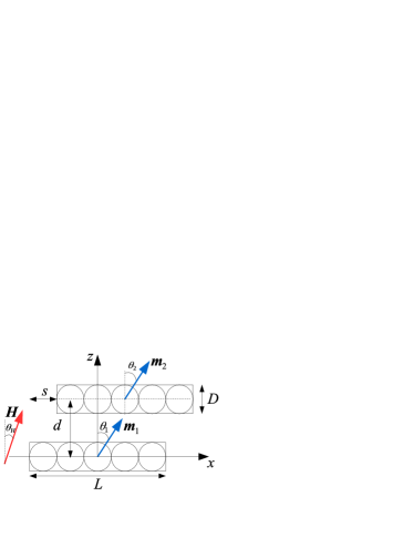
Figure 1: Two coupled chains of identical magnetic nanoparticles in a transverse magnetic field $\bm{H}$.

II.1 Magnetostatic interaction : beyond the point-dipole approximation

Our system consists of two chains of nanoparticles, assumed to lie in the $xz$ plane: chain 1 lies on the $x$-axis and extends from $-L/2$ to $+L/2$ and chain 2 is parallel to the first chain with separation $d$ in the $z$-direction and is shifted a distance $s$ along the $x$-axis; it lies from $(-L/2+s,d)$ to $(L/2+s,d)$, see Fig. 1.

Inside the chain, the magneto-crystalline anisotropy and shape anisotropy (for a cylinder with demagnetizing factors $N_{z}=0$, $N_{x}=N_{y}=\frac{1}{2}$) add up to induce a strong effective anisotropy along the chain’s axis with constant $K_{{\rm eff}}$. The magnetic field $\bm{H}$ is of variable amplitude and direction and is applied in an arbitrary direction with respect to the chain’s axis. This allows for the calculation of the resonance frequency as a function of the field amplitude and the resonance field as a function of the field direction. Consequently, the energy of a single chain reads (in dimensionless units)

$$\mathcal{E}\equiv E/\left(K_{{\rm eff}}V\right)=-2\bm{h}\cdot\bm{m}-km_{x}^{2}$$ (1)

where $h=\mu_{0}HM_{s}/2K_{{\rm eff}}V$. ${\bf M}=M_{s}\bm{m}$, where $M_{s}$ is the material’s saturation magnetization and $\bm{m}$ the unit vector along the (equilibrium) magnetization direction, $V=L\times\pi R^{2}$ is the volume of the cylindrical chain. The symbol $k$ in Eq. (1) is inserted as a flag to identify the anisotropy contribution and it assumes the value $0$ in the absence of anisotropy and $1$ otherwise.

In addition to the single-chain terms in the energy, chains 1 and 2 are coupled by the DI. We denote by ${\bf M}_{1}=M_{s}\bm{m}_{1}$ and ${\bf M}_{2}=M_{s}\bm{m}_{2}$ the two magnetic moments of the two chains. In the limit of homogeneous chains with the magnetization aligned along the chains axis, Escrig et al. (Escrig et al., 2008) have shown that the interaction energy can be rewritten in the compact form $E_{\mathrm{int}}=\eta_{\mathrm{int}}\,\bm{m}_{1}\cdot\bm{\mathcal{D}}\bm{m}_{2}$, where $\bm{\mathcal{D}}$ is the usual dipolar tensor with matrix elements $\mathcal{D}^{\alpha\beta}=\delta^{\alpha\beta}-3e_{12}^{\alpha}e_{12}^{\beta}$, where $\delta^{\alpha\beta}$ is the Kronecker symbol and $e_{12}^{\alpha}$ are the Cartesian components of the unit vector ${\bf e}_{12}$ joining the centers of the chains. Finally, $\eta_{\mathrm{int}}$ is the coefficient of the DI between two nano-chains as defined in Eq. (4) of Ref. Escrig et al., 2008.

In the present work, we consider the general case involving anisotropy and an applied magnetic field with arbitrary orientation. Therefore, the magnetic moments ${\bf M}_{1}$ and ${\bf M}_{2}$ may adopt orientations that are not necessarily collinear with each other and/or with the chains axes. Thus, we derive the dipolar tensor for this general situation. For this purpose, we regard each chain as being made up of elementary magnetic moments $d\bm{M}_{i}=\lambda dx_{i}\bm{m}_{i}$, where $\lambda$ is the linear density of dipoles ($\lambda dx=M_{s}dV$), $dx_{i}$ the differential element along the chain and $\bm{m}_{i}$ is the unit vector along the magnetic moment of the chain. Since we are dealing with chains ($L\gg R$), the magnetization $d\bm{M}_{i}$ associated with the differential element $dx_{i}$ can be considered as being radially uniform. If we use the index $i$ to label these elements in chain $1$ and $j$ those in chain $2$, the corresponding elements $d\bm{M}_{i}$ and $d\bm{M}_{j}$ can be considered as point dipoles interacting via the well-known dipole-dipole interaction

$$dE_{\mathrm{int}} = \frac{\mu_{0}}{4\pi}\frac{d\bm{M}_{1}\cdot d\bm{M}_{2}-3\left(d\bm{M}_{1}\cdot{\bf e}_{12}\right)\left(d\bm{M}_{2}\cdot{\bf e}_{12}\right)}{r_{12}^{3}}$$

$$= \frac{\mu_{0}}{4\pi}\lambda^{2}dx_{1}dx_{2}\frac{\bm{m}_{1}\cdot\bm{m}_{2}-3\left(\bm{m}_{1}\cdot{\bf e}_{12}\right)\left(\bm{m}_{2}\cdot{\bf e}_{12}\right)}{r_{12}^{3}}$$

with

$$\bm{r}_{12} = d\bm{e}_{z}+\left(x_{2}-x_{1}\right)\bm{e}_{x},\quad r_{12}=\left[d^{2}+\left(x_{2}-x_{1}\right)^{2}\right]^{1/2},$$

$$\bm{e}_{12} \equiv \frac{\bm{r}_{12}}{r_{12}}=\frac{d}{r_{12}}\bm{e}_{z}+\frac{\left(x_{2}-x_{1}\right)}{r_{12}}\bm{e}_{x}.$$

Next, upon integrating over the (length of) chains with the corresponding variables $x_{1},x_{2}$ in the ranges $-\frac{L}{2}\leq x_{1}\leq\frac{L}{2},-\frac{L}{2}+s\leq x_{2}\leq\frac{L}{2}+s$, we obtain the energy of the DI, taking account of the size and shape of the chains through the length and the chains separation $d$. More precisely, this interaction energy can be rewritten for arbitrary orientations of the two magnetic moments $\bm{m}_{1},\bm{m}_{2}$ as $\mathcal{E}_{\mathrm{int}}=\xi\bm{m}_{1}\cdot\tilde{\mathcal{\bm{D}}}\cdot\bm{m}_{2}$ where

$$\tilde{\mathcal{\bm{D}}}=\left(\begin{array}[]{ccc}\mathcal{I}_{03}-3\mathcal{I}_{25}&0&-3d\mathcal{I}_{15}\\ 0&\mathcal{I}_{03}&0\\ -3d\mathcal{I}_{15}&0&\mathcal{I}_{03}-3d^{2}\mathcal{I}_{05}\end{array}\right)$$ (3)

is the new DI tensor and

$$\xi=\frac{1}{K_{{\rm eff}}V}\times\left(\frac{\mu_{0}}{4\pi}\right)\left(\frac{\lambda^{2}}{d}\right)$$

the new (dimensionless) DI coefficient. The matrix elements in Eq. (3) are given by the surface integrals: $\mathcal{I}_{03}=\Theta\left(L,s\right)$, $\mathcal{I}_{05}=2\Theta\left(L,s\right)-\Phi\left(L,s\right)$, $\mathcal{I}_{15}=\frac{s}{d}\Phi\left(L,s\right)+\frac{L}{d}\left[B^{-1}\left(L,s\right)-B^{-1}\left(L,-s\right)\right]$ and $\mathcal{I}_{25}=\Theta\left(L,s\right)+\Phi\left(L,s\right)$, with $B\left(L,\pm s\right)=\sqrt{1+\left(L\pm s\right)^{2}/d^{2}}$ and $\Theta\left(L,s\right)=B\left(L,s\right)-2B\left(0,s\right)+B\left(L,-s\right)$, $\Phi\left(L,s\right)=B^{-1}\left(L,s\right)-2B^{-1}\left(0,s\right)+B^{-1}\left(L,-s\right)$.

Note that $\xi$ is a function of the materials saturation magnetization $\lambda$ and the chains separation $d$. However, in the results shown later the DI intensity will be tuned by varying either $d$ or $\xi$ directly. Therefore, the total energy of the system of two (shifted) chains reads

$$\mathcal{E}=\sum_{i=1,2}\left(-2\bm{h}\cdot\bm{m}_{i}-km_{x,i}^{2}\right)+\xi\bm{m}_{1}\cdot\tilde{\mathcal{\bm{D}}}\bm{m}_{2}.$$ (4)

Note that, for convenience, the DI coefficient $\xi$ has been defined with a dependence on the chains separation as $1/d$. However, the whole DI term of $\mathcal{E}$ behaves as $1/d^{3}$, as usual, owing to the dependence on $d$ of the integrals appearing in the matrix elements of the DI tensor $\tilde{\mathcal{\bm{D}}}$. In addition, the particular form of these matrix elements is a result of the specific shape of the elements (here the chains). Therefore, the DI energy found here with the tensor in Eq. (3) take account of the size and shape of chains, in addition to their separation.

II.2 Magnetic state of an isolated chain

Before proceeding further we would like to comment on the validity of the model used here for the magnetic state of the isolated chains (of nanoparticles) or nanowires. More precisely, we assume that each chain is a single domain cylinder (or a prolate spheroid) with uniform magnetization pointing along the chain’s axis due to the large shape anisotropy. The magnetostatic interaction between the two chains is dealt with using a general approach for computing the demagnetizing tensor for uniformly magnetized elements of finite-size and arbitrary shape. This approach extends the so-called point-dipole approximation which consists in replacing the magnetic elements (here the chains) by point dipoles. In fact, this assumption fails for finite-size elements with a too small separation between them and this is why one has to extend the magnetostatic interaction by including adequate geometrical factors (M. Beleggia S. Tandon, Y. Zhu, and M. De Graef, 2004; M. Beleggia, S. Tandon, Y. Zhu, and M. De Graef, 2004; A. F. Franco, J. L. Déjardin, and H. Kachkachi, 2014), as is done in Eqs. (3, 4).

There is a huge number of studies on arrays of ferromagnetic nanowires owing to their promising applications in high-frequency devices. They have been extensively studied both experimentally and theoretically (Velazquez et al., 1999; Sampaio et al., 2000; Thurn-Albrecht et al., 2000; Demand et al., 2002; Li et al., 2004; Zhan et al., 2005; Nguyen et al., 2006; Wang et al., 2006; Clime et al., 2006; Piccin et al., 2007; Kartopu et al., 2009; Medina et al., 2009; Stashkevich et al., 2009; Vidal et al., 2009; Ott et al., 2009; Maurer et al., 2009; Zighem et al., 2011; Rando and Allende, 2015) with variable length and width. The theoretical work is mainly based on the numerical approach of micromagnetics or semi-analytical approaches for solving the extended magnetostatic model. In all of these works, the magnetization is considered as uniform even in the largest nanowires (or rather microwires) of an aspect ratio within the range of fabrication techniques. For example, in Ref. Piccin et al., 2007 nanowires of radius $R$ and length $L$ were studied and even for $R/L$ of order $10^{-4}$ the magnetization within the nanowires was assumed to be uniform. It was then shown that the extended model of magnetostatic interactions reproduces very well the experimental results, see for instance Fig. 3 of Ref. Piccin et al., 2007. The same conclusion regarding the validity of this model was reached in other works comparing theory to the results of other experiments Zhan et al., 2005; Clime et al., 2006; Kou et al., 2009. In particular, in Refs. Kou et al., 2009; Boucher et al., 2011, FMR expriments on arrays of nanowires were performed and their results were favorably compared to the extended magnetostatic model. In these works, the assembly of nanowires was treated as being organized into two groups having their uniform magnetization pointing up and down.

In the present study, the aspect ratio of the chains is $R/L=0.05$. In addition, the effective anisotropy is dominated by the magnetostatic (shape) anisotropy with an easy axis along the chain and a constant $K_{{\rm eff}}\simeq 1.6\times 10^{6}\,\mathrm{J.m}^{-3}$. These specifications put on the safe side the assumption of uniform magnetization with an easy direction along the chain’s axis. In other words, the chains are magnetically saturated along their axes. This is obviously more so in the case of an external magnetic field applied along the chains. In the present study the direction of the magnetic field is varied with respect to the chains axes. In order to ensure that the assumption of uniform magnetization still applies even in the most unfavorable situation of a field applied perpendicular to the chains axis, we have performed numerical calculations for (isolated) chains of 10 spherical nanoparticles along the $z$-axis, as shown in the inset of Fig. 2. The nanoparticles constituting each chain have a diameter $D=20\ {\rm nm}$ and an (effective) easy anisotropy axis along the chain. Within the chain the nanoparticles interact with each other via the long-range DI with strength $\xi_{{\rm intra}}=\left(\frac{\mu_{0}}{4\pi}\right)\frac{\pi}{6}M_{s}^{2}/K_{{\rm eff}}$, which evaluates to $\xi_{{\rm intra}}\simeq 0.17$ for iron ($M_{s}=1.7\leavevmode\nobreak\ 10^{6}\ {\rm A.m^{-1}}$). In Fig. 2 we plot the deviation angle of the individual magnetic moments of the nanoparticles within the chain as a function of their position in the chain.

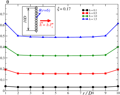
Figure 2: Deviation angle $\theta$ of the magnetization of each nanoparticle as a function of its position in the chain. Inset: single chain setup consisting of 10 nanoparticles forming a chain along the $z$-axis with tranverse external field $h$, the deviation angle $\theta$ is shown in blue for the 6th nanoparticle of the chain.

It is clearly seen that even in a transverse magnetic field the magnetic moments within the chain tilt towards the field direction in unison apart from a small number of them located at and near the chain’s ends. However, the relative deviation of these boundary moments is rather small. Similar results were obtained from micromagnetic calculations in Ref. Zighem et al., 2011. This result is due to the fact that, within the chain, the dipolar interactions favor the (super)ferromagnetic state as they induce an extra anisotropy along the chain. More precisely, they renormalize the anisotropy as $k\to k_{{\rm eff,DI}}$. The idea underlying this renormalization can be illustrated by considering a chain of $\mathcal{N}$ free nanoparticles with a uniaxial anisotropy $k$ and a transverse external field $h$, in the absence of DI. The deviation angle at equilibrium is then given by $\sin\theta_{{\rm eq,Free}}=h/k$. For low-to-intermediate magnetic fields, the deviation angle remains small, such that $\sin\theta_{{\rm eq,Free}}\simeq\theta_{{\rm eq,Free}}$. In this case, after switching on the DI the deviation angle can be self-consistently determined to first order in $\xi_{{\rm intra}}$. Indeed, it can be shown that it is given by $\theta\left(r_{i}\right)=h/k_{{\rm eff,DI}}\left(r_{i}\right)$, where $k_{{\rm eff,DI}}$ depends only weakly on the position $r_{i}$ within the chain since $k_{{\rm eff,DI}}\simeq k\left[1+3\xi_{{\rm intra}}I\left(r_{i}\right)\right]$. The lattice sum $I\left(r_{i}\right)$ stems from the intra-chain DI between a particle and all the other ones within the chain (i.e. those on its left and its right), namely

$$I\left(r_{i}\right)=\sum_{j=1}^{i-1}\frac{1}{\left(r_{i}-r_{j}\right)^{3}}+\sum_{j=i+1}^{\mathcal{N}}\frac{1}{\left(r_{j}-r_{i}\right)^{3}}.$$ (5)

The symmetry of the expression above translates into the symmetry of the deviation angle depicted in Fig. 2. We note in passing that for a chain of 10 spherical nanoparticles, we obtain the effective anisotropy $k_{{\rm eff,DI}}\simeq 2k$, which exceeds the largest value of the magnetic field used in Fig. 2.

To sum up, these additional calculations do confirm that the magnetization within an (isolated) chain may be reasonably regarded as uniform even in a transverse magnetic field. On the other hand, for the magnetostatic interaction between the two chains, we have developed an extended model with a new magnetostatic tensor [see Eq. (3)] that takes into account the finite size and shape of the interacting nano-elements.

In the following we present and discuss our results for the system of two coupled chains as described above.

III Results

III.1 FMR characteristics

The FMR characteristics, namely the resonance frequency and resonance field, are computed as follows. For a given system configuration (including anisotropy, applied field and spatial configuration of the two chain), we first determine the equilibrium state of the system, i.e. the spatial orientation of the two (macroscopic) magnetic moments of the chains. Then, we linearize the Landau-Lifshitz equation around this state leading to an eigenvalue problem for the system. Upon solving the latter for a given applied magnetic field (with given amplitude and direction) we obtain the various eigenfrequencies of the excitation modes of the coupled two chains. Next, for a fixed frequency we solve the eigenvalue problem for the applied magnetic field and this renders the resonance field.

Now, we proceed to compute the resonance frequency $\omega_{{\rm res}}$ and the flipping field $h_{f}$ of the system whose total energy is given in Eq. (4). We first compute the resonance frequency for the case of zero shift ($s=0$) between the two chains as this leads to tractable analytical expressions. For the general case, $\omega_{{\rm res}}$ and $h_{f}$ will be computed numerically, respectively as a function of the field amplitude $h$ and the field direction $\left(\theta_{h},\varphi_{h}\right)$.

For the non-shifted chains, the analytical calculation of $\omega_{{\rm res}}\left(h\right)$ is done for the setup with $\theta_{h}=0,\varphi_{h}=0$. In the present case, the two anisotropy axes and the applied magnetic field are all in the $zx$ plane, and as such the magnetic moments also lie in the same plane, i.e. we have $\bm{m}_{i}\left(\theta_{i},\varphi_{i}=0\right)$.

In the absence of anisotropy and applied field, the DI favors a ferromagnetic order of the two magnetic moments along the dimer’s bond, i.e. along the $z$ axis. If the effective uniaxial anisotropy is added with easy axis along the chains, the two magnetic moments order anti-ferromagnetically along the $x$ axis. Finally, when the magnetic field is applied along the $z$ axis, the two magnetic moments are tilted to an oblique angle that depends on ($h,\xi$), i.e. a canted anti-ferromagnetic state. Upon analyzing the energy stationary points, it turns out that there are two field regimes separated by the critical value $h_{c}=k\left[1-\tilde{\xi}\left(\delta^{2}+a\right)\right]$, where $a=1-\sqrt{1+\delta^{2}}$ and $\delta=L/d$ and $\tilde{\xi}=\xi/\left(k\sqrt{1+\delta^{2}}\right)$. More precisely, the polar angles of the two magnetic moments are $\theta_{1}=-\theta_{2}=\theta^{\left(\mathrm{m}\right)}$ with $\cos\theta^{\left(\mathrm{m}\right)}=h/h_{c}$ for $h\leq h_{c}$ (and $\theta^{{\rm(m)}}=0$ otherwise). This result obviously coincides with that obtained in Ref. A. F. Franco, J. L. Déjardin, and H. Kachkachi, 2014, Eq. (37) after a rotation of the frame axes and noting that for point dipoles $\delta=L/d$ becomes small and that the quantity $\left(\frac{\mu_{0}}{4\pi}\right)\left(\lambda L\right)^{2}/d^{3}$ is the DI coefficient in Ref. A. F. Franco, J. L. Déjardin, and H. Kachkachi, 2014.

For $h\leq h_{c}$, we obtain the following analytical expressions for the resonance frequencies of the binding (B) and anti-binding (AB) modes,

$${\normalcolor{\color[rgb]{0,0,1}{\normalcolor\tilde{\omega}_{\mathrm{B}}}}} = \left(2k\right)\sqrt{1-\left(h/h_{c}\right)^{2}}\times\sqrt{\left(h_{c}/k\right)\left[1-\left(2a+\delta^{2}\right)\tilde{\xi}\right]},$$

$${\color[rgb]{0,0,1}{\normalcolor\tilde{\omega}_{\mathrm{AB}}}} = \left(2k\right)\sqrt{\left[1+\left(\delta^{2}-a\right)\tilde{\xi}\right]-\left(h^{2}/h_{c}^{2}\right)\left[1+\left(\delta^{2}+a\right)\tilde{\xi}\right]}$$ (6)

$$\times\sqrt{1+\delta^{2}\tilde{\xi}}.$$

Here $\tilde{\omega}$ is the dimensionless frequency defined by $\tilde{\omega}\equiv\omega/\omega_{{\rm a}}$, where $\omega_{{\rm a}}=\gamma H_{a}$ with $H_{a}$ being the anisotropy field given by $H_{a}=2K_{{\rm eff}}/M_{s}$. For the material parameters given earlier, our reference frequency is then $\nu_{a}=\omega_{{\rm a}}/2\pi\simeq 52\,{\rm GHz}$.

For non interacting chains one recovers the well known result of two degenerate modes with the frequency $\tilde{\omega}_{\mathrm{B}}=\tilde{\omega}_{\mathrm{AB}}=\left(2k\right)\sqrt{1-\left(h/k\right)^{2}}\equiv\tilde{\omega}^{\left(0\right)}$. By inspection of Eq. (6), we see that for small $\xi$ and $h$ the frequency of the anti-binding mode is higher than that of the binding mode because it corresponds to an out-of-phase precession of the magnetic moments as seen in Fig. 3.

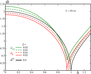
Figure 3: Resonance frequencies of the binding (red) and anti-binding (green) modes for non shifted chains, for different ${\normalcolor\xi}$.

For $h>h_{c},$ the resonance frequencies are given by

$$\tilde{\omega}^{\prime}_{\mathrm{B}} = 2h\sqrt{\left(1-\frac{a\tilde{\xi}}{h}\right)}\sqrt{1-h_{c}/h},$$ (7)

$$\tilde{\omega}^{\prime}_{\mathrm{AB}} = 2h\sqrt{1+\frac{\left(a+2\delta^{2}\right)\tilde{\xi}}{h}}\sqrt{1-\frac{h_{c}+2a\tilde{\xi}}{h}}.$$

In Fig. 3 we observe a shift (downwards) of the critical field $h_{c}$ at which (only) the binding modes vanishes as the intensity of the DI increases. This is obviously recovered by the expression $h_{c}$ of the critical field given above. The reason for this effect is that the energy minimum, with $\cos\theta^{\left(\mathrm{m}\right)}=h/h_{c}$, is a result of the competition between the anisotropy and the combined effect of the applied field and the DI. Thus, when the latter becomes stronger, a weaker field is needed to overcome the effect of the anisotropy.

In Fig. 4 we show the effect on the frequency of the anti-binding mode of a shift of the chains with respect to each other along their axes.

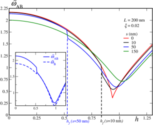
Figure 4: Resonance frequency $\tilde{\omega}_{{\rm AB}}$ for shifted chains. The inset shows the binding and anti-binding modes for ${\normalcolor s=50\ {\rm nm.}}$

These results show that for a given shift between the two chains, there appears a jump in the resonance frequency of the anti-binding mode - that of the binding mode also exhibits such a jump (but less pronounced) for the same value of the $h_{f}$ (Inset in Fig. 4). This jump can be understood as follows. For very small fields, the equilibrium state is an anti-ferromagnetic ordering of the two magnetic moments along the anisotropy axes. As the field is increased, there is a transition into a ferromagnetic state in an oblique direction with respect to the applied field. It is this transition that is responsible for the abrupt change in the resonance frequency. A further increase of the magnetic field leads to the saturation state and thereby to the asymptote in the form of a straight line ($h\geq h_{c}$). As the shift of the two chains increases, the field at which this jump occurs (we call it the spin-flop field $h_{f}$) decreases. Indeed, as the shift is increased, the dimer’s bond tilts towards the chain axes and thereby the two magnetic moments tend to order along the anisotropy easy axes. In this case the ferromagnetic order is more favorable and this is why the field amplitude required to trigger the transition from the anti-ferromagnetic to ferromagnetic order is smaller. The system then rotates towards the direction of the applied field as a single (larger) magnetic moment. For a large shift, the system is in a ferromagnetic order already at zero field, see the green curve in Fig. 4.

For a magnetic field applied in the $z$ direction ($\theta_{h}=0$), the black curve in Fig. 5 clearly illustrates the decrease of the field $h_{f}$ as a function of the chain shift $s$. As soon as the applied magnetic field is tilted with respect to the $z$ direction ($\theta_{h}\neq 0$), the field $h_{f}$ at which the transition between the two ordered states occurs reduces significantly.

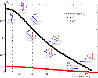
Figure 5: Flipping magnetic field $h_{f}$ marking the “spin flop” transition as a function of the chains shift, for two field directions and for ${\normalcolor\xi=0.02}$. For $\theta_{h}=0\text{$\textdegree$}$, the magnetic moments are drawn in blue for various shifts below and above the “spin-flop” transition.

This evolution is clearly seen in Fig. 5, where we compare the evolution of the direction of the two magnetic moments for $\theta_{h}=0\text{$\textdegree$}$ and $10\text{$\textdegree$}$. First, as we go vertically through the $h_{f}$ curve, at a given shift $s$, we observe the switching of one of the two magnetic moments: the $x$-component of the moments switches from an anti-ferromagnetic to a ferromagnetic order. Second, as we increase $s$ we see that the canting angle of the “anti-ferromagnetic” order, in the phase with $h<h_{f}$, becomes larger ending up in a nearly complete anti-ferromagnetic order along the anisotropy axis. Finally, as discussed above, beyond some critical value of the shift, that depends on $L$ and $d$, there is only one phase corresponding to the ferromagnetic order. The maximum critical shift $s_{0}$ corresponding to $h_{f}=0$ (e.g. in Fig. 5 $s_{0}\sim 129{\rm nm}$) can easily be predicted as a function of $L$ and $d$. Indeed, if one considers ferromagnetic and anti-ferromagnetic states fully polarized along $x$ on either side of this point, the DI energies of these states should be the same at the transition. Hence, $s_{0}$ is the root of the equation $\Phi\left(L,s_{0}\right)=0$, which implies that the interaction coefficient $\eta_{{\rm int}}$ vanishes (i.e. DI$\to 0$). As we intuitively expect, $s_{0}$ increases as $d$ or $L$ increases.

Finally, in FMR experiments one routinely obtains the resonance field as a function of the direction of the applied magnetic field. The corresponding data is an efficient means for characterizing the system with regards to the easy/hard magnetization directions. So it is worthwhile to compute this observable for our system and to investigate the effect of a chains relative shift. Accordingly, we have (numerically) computed the resonance field as a function of the applied field polar angle $\theta_{h}$ upon varying the spatial shift and inter-chains separation (or DI strength). The results are shown in Fig. 6.

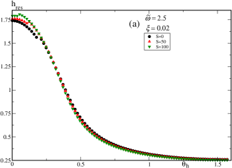
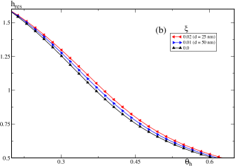
Figure 6: Resonance field against the applied field polar angle $\theta_{\mathrm{h}}/\pi$, for variable spatial shift (a) and inter-chains separation with $s=0$ (b).

It can be seen that the resonance field exhibits the usual overall behavior as a function of the applied field direction, as the latter rotates from the anisotropy easy axis to the hard axis (A.G. Gurevich and G.A. Melkov, 1996). On the other hand, in the present study the resonance field shows a weak dependence on the spatial shift $s$, whereas its dependence on the inter-chains separation $d$ follows the expected behavior. More precisely, for small angles $\theta_{h}$ the applied field competes with the DI and this leads to higher resonance fields for higher DI strengths (or smaller separation $d$).

IV Conclusions

We have computed the FMR characteristics of a system of two coupled chains, taking into account their separation and relative shift. The DI has been dealt with taking into consideration their finite size and shape. We have found that the shift of the two chains along their axes has a significant effect on the resonance frequency. More precisely, as the magnitude of the magnetic field is increased the system goes through a “spin-flop” transition from an anti-ferromagnetic order to a ferromagnetic order before reaching the high-field branch of the resonance frequency. The field that marks this transition decreases with an increasing shift of the chains and depends on the systems specifications such as the length of the chains, their separation and the orientation of the magnetic field. This field defines magnetic regions of importance for magnetic recording media made of 1D nanoelements.

We have also computed the resonance field as a function of the magnetic field direction for varying inter-chain separation and spatial shift. The resonance field is what is routinely measured in FMR measurements with a rotating applied magnetic field and allows for characterizing the system with regards to its physical parameters. In the present study, this could be useful for characterizing, inter alia, the magnetostatic interaction between the chains.

Finally, the present study, restricted to a dimer, allows one to fully investigate the critical shift as a function of the applied field (which mimics the write/read process), and sets the stage for further investigation involving dimer assemblies. The latter could in principle be tackled numerically using the present approach by summing over pairs with the effective DI derived here.