Superfluid density and quasi-long-range order in the one-dimensional disordered Bose-Hubbard model

Abstract

We study the equilibrium properties of the one-dimensional disordered Bose-Hubbard model by means of a gauge-adaptive tree tensor network variational method suitable for systems with periodic boundary conditions. We compute the superfluid stiffness and superfluid correlations close to the superfluid to glass transition line, obtaining accurate locations of the critical points. By studying the statistics of the exponent of the power-law decay of the correlation, we determine the boundary between the superfluid region and the Bose glass phase in the regime of strong disorder and in the weakly interacting region, not explored numerically before. In the former case our simulations are in agreement with previous Monte Carlo calculations.

1 Introduction

The Bose-Hubbard model is a widespread paradigm in the field of strongly-correlated many-body systems [1]. Over the years it has found applications in the physics of superconducting thin-films [2], Josephson junction arrays [3], optical cavity arrays [4], and cold atoms in optical lattices [5]. The model describes bosons hopping on a tight-binding lattice and interacting through an on-site repulsion. The non-trivial properties of the model stem from the competition between the hopping (that delocalizes the particles) and the local repulsion (that tends to suppress local particle number fluctuations). In the absence of disorder such a competition dictates a quantum phase transition at integer filling: if the hopping dominates, the ground state of the system is superfluid; in the opposite regime, there is a gap in the excitation spectrum and the system is in a Mott insulating state. At a critical value of the ratio between the hopping and the repulsion parameters, an insulator to superfluid quantum phase transition takes place at zero temperature. In optical lattices this transition has been experimentally demonstrated in the seminal work by Greiner et al. [6]. The phase diagram of the Bose-Hubbard model has been studied by a number of analytical and numerical methods, a recent account of the properties of this model together with a review of the experimental advances with cold atoms can be found in the reviews [7, 8].

In one dimension (1D), which is the case of interest for the present work, the quantum phase transition between the Mott insulating (MI) phase and the superfluid (SF) phase at fixed commensurate lattice filling is known to be of the Berezinkii-Kosterlitz-Thouless (BKT) type [1]. The critical properties of the quantum model map onto that of a classical two-dimensional $XY$ model. The hallmark of a BKT transition [9, 10, 11] is a universal jump [12] in the superfluid density (or stiffness or helicity modulus [13]). Extensive studies of the stiffness in the classical 2D $XY$ model are reported for example in [13, 14]. Monte Carlo simulations of the one-dimensional quantum model (the mapping onto the $XY$ model becomes accurate at large fillings) were performed originally in [15], more recent results are comprehensively discussed in [16]. On the other hand, the Density Matrix Renormalization Group alias Matrix Product States (MPS) [17] has been applied to the model under consideration [18, 19, 20, 21], although the superfluid stiffness is difficult to extract with high precision because these methods are not ideally suited to deal with periodic boundary conditions (PBC) [22].

The presence of disorder enriches the phase diagram with a new phase, the Bose glass (BG) [1], surrounding a superfluid lobe in the interaction vs. disorder plane of the phase diagram. In absence of interactions, indeed, the disorder induces Anderson localization of single particle states and therefore an insulating phase. This is then lifted by a moderate amount of interactions that tend to reestablish coherence and consequently superfluidity. At large interactions and large disorder, finally, strong correlations should lead back to an insulating phase, distinct from the above mentioned Mott insulator in the clean setup. Although this picture is qualitatively well-understood, the full quantitative characterization of the disordered Bose-Hubbard model remains challenging: considerable efforts have been devoted to study its phase diagram, in particular the location and the nature of the glassy phase [23, 24, 25, 26, 27, 28, 29, 30, 31, 32, 33, 34]. Developments on the issue, with a special emphasis on numerical simulations, have been reviewed in [35]. Recently, an experiment with optical lattices has made an important step forward in mapping the phase diagram from weak to strong interactions [36].

In the present work we apply a Tree Tensor Network (TTN) method [37, 38, 39, 40, 41] (specifically our recently introduced gauge-adaptive TTN technique [42]), a natural ansatz for the simulation of one-dimensional quantum many-body systems with PBC, to the disordered Bose-Hubbard model. We compute the superfluid stiffness and correlation functions, avoiding the detrimental boundary effects arising in simulations with open boundary conditions. Furthermore, by analyzing the statistics of the decay of superfluid correlators we are able to locate the superfluid to Bose glass transition line, to extend it into the previously numerically unexplored regime of small on-site interactions, and to confirm the Monte Carlo results of Ref. [26] for strong interactions.

The paper is organized as follows: In the next section we introduce the model and give a brief overview of the used numerical technique (a detailed discussion can be found in [42]) and we anticipate the main result of the paper, the phase diagram of the disordered BH model at unit filling. In section 3 we analyze the superfluid stiffness. As a benchmark we first consider the case without disorder where we are able to perform a very accurate finite-size scaling to locate the BKT transition. We compare the obtained transition point with the results from other well-known methods for determining the MI-SF transition, such as numerically extracting the Luttinger parameter from the hopping correlation functions [18], finding very good agreement. Moreover, we present our results for the average stiffness in the disordered case. In order to get a precise location of the transition points we study the hopping correlation decay, as presented in section 4. A detailed analysis of the statistics of the exponent of the power-law decay allows us to map out the complete SF-BG transition line in the phase diagram. Finally, we summarize the main results of the work in section 5.

2 The disordered Bose-Hubbard model

The one-dimensional Bose-Hubbard model is a system of spinless bosons moving in a single-band tight-binding lattice, described by the Hamiltonian

$${\cal H}=-t\sum_{j}\left(b_{j}^{\dagger}b_{j+1}+\mathrm{h.c.}\right)+\frac{U}{2}\sum_{j}n_{j}(n_{j}-1)-\sum_{j}V_{j}n_{j}\;.$$ (1)

The first term accounts for the hopping between neighboring sites (labeled by the index $j$), the second for the on-site repulsion and the last for the effect of a random inhomogeneous chemical potential. The couplings $t$, $U$ and $V_{j}$ are the hopping amplitude, the on-site repulsion, and the random potential, respectively; $b_{j}$ ($b^{\dagger}_{j}$) are bosonic annihilation (creation) operators obeying $[b_{j},b^{\dagger}_{j\prime}]=\delta_{jj^{\prime}}$, with $n_{j}=b^{\dagger}_{j}b_{j}$ being the corresponding number operators. The random on-site disorder $V_{j}$ is independent on different sites and uniformly distributed in the interval $[-\Delta,\Delta]$.

In order to compute the stiffness we introduce a twist $\phi$ in the boundary conditions. This amounts to considering periodic boundary conditions and performing a Peierls shift in every hopping matrix element

$$t\,\left(b_{j}^{\dagger}b_{j+1}+\mathrm{h.c.}\right)\;\;\longrightarrow\;\;t\,\left(b_{j}^{\dagger}b_{j+1}\;\mathrm{e}^{-2\pi i\phi/N_{s}}+\mathrm{h.c.}\right)$$

where $N_{s}$ is the number of sites of the ring, as schematically depicted in Fig. 1 a) where the twist is explicitly interpreted as a magnetic flux $\phi$ piercing the ring and acting on electrically charged particles.

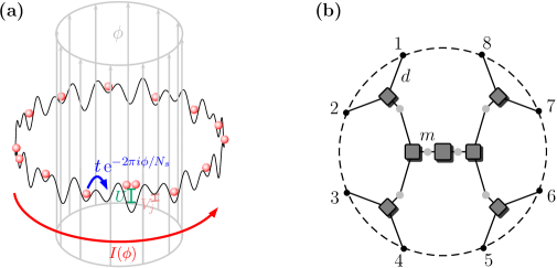
Figure 1: (a) Sketch of a Bose-Hubbard ring with hopping $t$, on-site interaction $U$ and local disorder $V_{j}$ pierced by an external flux $\phi$, giving rise to a ground state boson current $I(\phi)\propto\partial E_{0}/\partial\phi$. (b) Sketch of the TTN state for a lattice with $N_{s}=8$ sites. The lattice sites (black dots) have a local dimension $d$. The three-legged tensors (gray squares, each leg represents a tensor index) hierarchically group two sites together, forming virtual sites (light gray dots). The dimension of the Hilbert space of the virtual sites is truncated at some maximum bond dimension $m$. A variational optimization of this RG scheme is then performed following the prescriptions introduced in [42].

Our TTN ansatz is sketched in Fig. 1 b), showing the natural capability to represent states on 1D lattices with PBC, despite its loop-free geometry. The absence of loops in the network is crucial for the applicability of efficient energy minimization techniques needed for the ground state search. For algorithm details we refer the reader to Ref. [42], however it is important to emphasize that with our TTN approach we will be able to compute the superfluid density for large system sizes (up to $N_{s}=256$ in the absence of disorder) and therefore perform a reliable finite-size scaling analysis. As we will show, at equilibrium in one dimension this approach provides matching results to Monte Carlo calculations.

The TTN algorithm we use has abelian global symmetries built-in [43], allowing us to work in a canonical ensemble (at zero temperature) by targeting exclusively $N$-particles states, in accordance with the $U(1)$ particle conservation symmetry $[{\cal H},\sum_{j}n_{j}]=0$ of the Hamiltonian ${\cal H}$. In the rest of the paper we will in particular consider the case of unit filling, i.e. $N=N_{s}$. We simulate system sizes of up to $N_{s}=256$ sites, with a truncated local boson basis up to a dimension of $d=20$ in the low $U$ regime where high local populations are possible. In the disordered scenario we average all observables over a number of $n_{r}=100$ different disorder realizations.

In Fig. 2 we anticipate the main result of this work, the phase diagram of the disordered BH model. The technical details and the discussion of the results are presented in the following sections, here we highlight that for strong interactions (the right edge of the lobe) our results obtained with three different criteria are in agreement with state-of-the-art Monte Carlo results. More interestingly, we are able to extend our numerical analysis into the low-interaction regime (left edge of the lobe): two independent criteria strongly agree down to values of the interactions of the order of $U\sim 0.4$, where the numerical results nicely match the theoretical conjecture for very small $U$ [35].

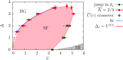
Figure 2: Phase diagram of the BH model with disorder in 1D at unit filling: Bose glass (white region), superfluid lobe (red region), Mott insulator (gray region). The boundaries of the SF lobe are determined via three different criteria: superfluid jump (green squares), Luttinger parameter $\overline{K}=2/3$ (red circles) and algebraic versus exponential decay of correlation functions (blue circles). The blue dashed line is a fit through the blue circles according to $\mu\,U^{\nu}$, with fit parameters $\mu=2.2\pm 0.1$ and $\nu=0.4\pm 0.1$ The red dashed line follows the conjectured behavior $\Delta_{c}\sim U^{3/4}$ of the phase boundary for $U\ll 1$ [35]. The gray shaded MI region is data from Ref. [26].

3 Superfluid stiffness

The superfluid stiffness $\rho_{s}$ is defined through the sensitivity of the ground state energy $E_{0}$ (here we consider the zero-temperature case) to a twist in the boundary conditions

$$\rho_{s}=\frac{N_{s}}{8\pi^{2}}\frac{\partial^{2}E_{0}}{\partial\phi^{2}}\bigg{|}_{\phi=0}\;,$$ (2)

and we set the energy scale by choosing $t=1$. Therefore, $\rho_{s}=1$ for vanishing on-site repulsion $U$ and vanishing disorder $\Delta$, while $\rho_{s}=0$ in the Mott-insulator and Bose glass phases.

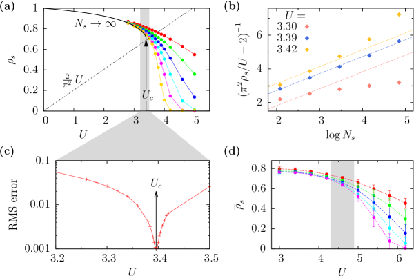
Figure 3: (a) Superfluid density $\rho_{s}$ as a function of on-site repulsion $U$ for various ring sizes $N_{s}=8,16,32,\ldots,256$ (from top to bottom) in the clean case $\Delta=0$. The arrow indicates the location and the height of the jump of $\rho_{s}$ in the thermodynamic limit, determined via Weber-Minnhagen fitting (shown in panel (b), dashed lines are fits). The resulting RMS errors for the gray-shaded interval of $U$ are shown in panel (c), where the pronounced minimum at $U_{c}=3.394\pm 0.03$ becomes apparent. (d) Averaged superfluid density $\overline{\rho}_{s}$ as a function of on-site repulsion $U$ for $\Delta=2.0$ in the disordered case. The error bars indicate the standard deviations of the $\rho_{s}$ distributions. The gray-shaded interval is the location of the critical point $U_{c}=4.6\pm 0.3$, determined via Weber-Minnhagen fitting.

As a benchmark of our approach, we first consider the clean case $\Delta=0$. At the BKT critical point the superfluid density jumps from a finite value $\rho^{c}_{s}$ to zero. The mapping onto the classical $XY$ model yields the critical value $\rho^{c}_{s}=\left(2/\pi^{2}\right)U_{c}$ in resemblance with the relation $P^{\,c}_{s}=\left(2/\pi\right)T_{c}$, known to hold for the classical XY model in 2D [12]. We determine the transition point $U_{c}$ by extracting the superfluid density as a function of the on-site repulsion $U$ for different ring sizes $N_{s}$. We then perform a Weber-Minnhagen fit according to the theoretically predicted functional dependence of the superfluid density at the BKT transition [13]:

$$\rho_{s}^{c}(N_{s})=\rho_{s}^{c}\left(1+\frac{1}{2}\frac{1}{\log N_{s}+b}\right)\;,$$ (3)

with $b$ the only fit parameter. When fitting $\rho_{s}(N_{s})=2U/\pi^{2}\,\left(1+[2\log N_{s}+b]^{-1}\right)$ for various $U$, the root-mean-square (RMS) error of the fit displays a pronounced minimum at the transition point [13]. Figs. 3 a)–c) show the result of this procedure, resulting in $U_{c}=3.394\pm 0.03$ (or, equivalently, $t_{c}/U=0.295\pm 0.003$).

We now introduce disorder and repeat the study for the averaged superfluid density $\overline{\rho}_{s}$. Since the SF-BG transition is also expected to be of the BKT type [23], at least on the right side of the SF lobe (i.e. at large $U$), $\overline{\rho}_{s}$ should display a jump at the phase transition in the thermodynamic limit. An example of our numerical results is shown in Fig. 3 d). In qualitative terms, for both sides of the lobe a drop of the superfluid density for increasing system sizes can be observed when entering the BG phase. Like in the clean system, we localize the critical point by means of a Weber-Minnhagen fitting procedure, this time with $\overline{\rho}^{c}_{s}$ as an additional fit parameter because the height of the jump for $N_{s}\rightarrow\infty$ is not known for arbitrary disorder. While on the right boundary of the SF lobe we are able to successfully apply this technique employing system sizes and disorder realization numbers accessible to our numerics, this is not the case on the left boundary. Here we do not achieve sufficient numerical precision to estimate a reliable minimum in the RMS error when fitting Eq. (3), which ultimately makes this method of determining the phase transition unfeasible for the small $U$ regime. This might be as well an indication of a different nature of the SF-BG phase transition in this regime, as proposed in some studies [35].

In order to continue with an accurate analysis of the critical SF-BG line in all regimes we study the superfluid correlations in the next section.

4 Correlation functions

We proceed further by studying the correlation functions, a method that turns out to yield higher accuracy in determining the transition line. Moreover, we double-check our results via another method for the determination of the MI-SF transition, namely the value of the Luttinger parameter $K$ obtained from the hopping correlation functions [18]

$$C(r)=\frac{1}{N_{s}}\sum_{j}\langle b^{\dagger}_{j}b_{j+r}\rangle\propto r^{-K/2}\;.$$ (4)

In the clean case the criterion for locating the BKT transition is given by $K_{c}=1/2$. Indeed, as critical exponents can be obtained with high numerical precision in TTN simulations [42], we expect this method to work well in the present scenario. Moreover, the PBC setting allows for an easy treatment of finite size effects in Eq. (4), simply by replacing the distance $r$ with the effective distance $\tilde{r}=\mathrm{crd}(r)$, where $\mathrm{crd}(r)=N_{s}/\pi\,\sin(\pi r/N_{s})$ is the chord function giving the effective distance of two sites $j$ and $j+r$ arranged on a regular polygon of $N_{s}$ edges. In A we demonstrate the validity of this procedure. Fig. 4 summarizes our numerical results, locating the transition at $t_{c}=0.299\pm 0.002$. Here, we set $U=1$ for the sake of an easy comparison with Ref. [18]; see Tab. 1 for how this compares to the transition points obtained in the literature.

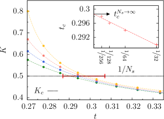
Figure 4: Determination of the clean ($\Delta=0$) BKT transition point via the Luttinger parameter criterion $K_{c}=1/2$. The highlighted interval on the $K_{c}$ line is the result obtained in Ref. [18]. The four different curves correspond to the four different system sizes $N_{s}=32,64,128,256$ (bottom to top). The inset shows an extrapolation of $t_{c}$ to the thermodynamic limit by means of a fit linear in $1/N_{s}$ (red dashed line), resulting in $t_{c}^{N_{s}\rightarrow\infty}=0.299\pm 0.002$. Errors due to finite bond dimension of the TTN state are smaller than the point size (see A for a convergence check).

We now once again turn back to the study of the disordered case. As already mentioned, this long-standing problem is unsolved in the low-interaction regime $U<2$, and even for the more easily tractable regime of higher interactions, results from different numerical methods are not in quantitative agreement [24, 26, 27, 35].

We start by studying the hopping correlation functions of Eq. (4), whose critical exponent gives access to the Luttinger parameter $K$. The Giamarchi-Schulz criterion $\overline{K}_{c}=2/3$ [47, 23], where the overline indicates an average over a number of $n_{r}$ disorder realizations, results in the phase boundary shown in Fig. 5. We remark that while the $\overline{K}_{c}=2/3$ criterion is known to be appropriate in the high $U$ regime [35], there is no definite evidence that this is also the case on the left boundary of the SF lobe (low $U$ regime). Therefore, the results of Fig. 5 require critical verification, which is presented in the following paragraphs.

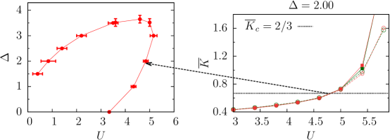
Figure 5: Extension of the SF lobe determined from the criterion $\overline{K}_{c}=2/3$ (left). The right panel shows the averaged Luttinger parameter $\overline{K}$ as a function of $U$ at fixed disorder $\Delta=2$, for two different ring sizes $N_{s}=64,128$ (circles, squares) and two different numbers of disorder realizations $n_{r}=50,100$ (green, red). In the low $U$ regime we used local dimensions of up to $d=20$ in order to account for possible high on-site occupations.

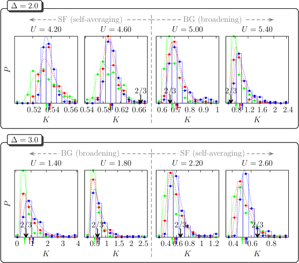
Figure 6: Behavior of the distributions of the Luttinger parameter $K$ across the SF-BG transition for different system sizes $N_{s}=32,64,128$ (green, red, blue), illustrated for two disorder strengths $\Delta=2$ (top panel) and $\Delta=3$ (bottom panel). Dashed lines are fits according to log-normal distributions Eq. (5), colored arrows indicate the corresponding mean values. Note the different scales on the abscissae to appreciate the clear difference between the self-averaging and broadening regimes. In all plots the number of disorder realizations is $n_{r}=100$. Increasing $n_{r}$ leaves the properties of the distributions unchanged within the statistical error, as we verify in B.

As a first step into this direction we study the distributions of the Luttinger parameter $K$ over disorder realizations. It has been shown [32] that in the SF phase the distributions display self-averaging, i.e. they become sharper and narrower for increasing system sizes. This is contrasted by a broadening and flattening in the BG phase [32, 48]. Therefore, the change between the two different types of behaviors should signal the SF-BG transition. Fig. 6 shows our analysis for two different values of the disorder strength: the first one contains the crossing of the right phase boundary when moving along the line $\Delta=2$, and the second one shows the crossing of the left phase boundary along the line $\Delta=3$. We find that the $K$-distributions are well captured by log-normal distributions with probability density

$$P(x)=\frac{1}{\sigma\sqrt{2\pi}}\,\frac{1}{x}\,\exp\left(-\frac{1}{2}\left(\frac{\log x-\mu}{\sigma}\right)^{2}\right)\;.$$ (5)

Here $x=K-K_{\mathrm{min}}$ (where $K_{\mathrm{min}}$ is the smallest measured $K$ value among the $n_{r}$ different disorder realizations), since $P(x<0)=0$ for log-normal distributions. The parameters $\mu$ and $\sigma$ determine the mean and the variance of the distribution. The results in Fig. 6 are consistent with the results in Fig. 5, meaning that we observe the crossover from self-averaging ($\partial[\mathrm{Var}(K)]/\partial N_{s}<0$) to broadening ($\partial[\mathrm{Var}(K)]/\partial N_{s}>0$) at locations compatible with the criterion $\overline{K}_{c}=2/3$.

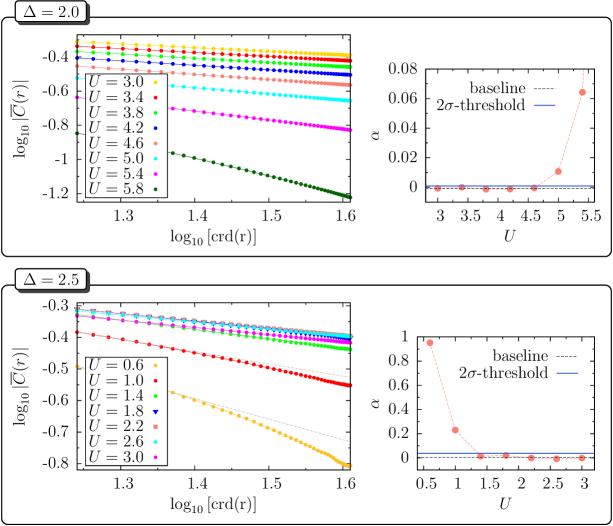
Figure 7: Determining the location of the SF-BG transition via the averaged hopping correlation functions. The left plots show the averaged correlation functions $\overline{C}(r)$ together with fits according to Eq. (6). The dashed gray lines are linear fits through the first five data points, serving as guides to the eye to discriminate the different scaling behaviors. The system size is $N_{s}=128$, the number of disorder realizations is $n_{r}=100$. Increasing $n_{r}$ does not result in changes bigger than the point size, the same applies for finite bond dimension effects. The extracted curvatures $\alpha$ as a function of $U$ are shown in the right plots. The baselines are determined as the average of the data points close to zero; the threshold is used to locate the critical points.

Finally, we propose a method for locating the SF-BG transition that requires minimal a priori knowledge on the nature of the transition, but merely relies on the assumption that the averaged hopping correlation functions $\overline{C}(r)$ (understood as an average of the correlation function $C(r)$ in Eq. (4) over all disorder realizations for each distance $r$) decay algebraically in the SF phase while in the localized BG phase they decay exponentially. We can conveniently discriminate the different scaling behaviors by fitting $\overline{C}(r)$ in double logarithmic representation with a function of the form

$$\log\left[\,\overline{C}(r)\right]=-\alpha\,\xi^{2}-\frac{K}{2}\,\xi+\mathrm{const.}\;,$$ (6)

where $\xi=\log\left[\mathrm{crd}(r)\right]$ and $\alpha$ is the curvature of the fit. Clearly, $\alpha=0$ indicates a straight line in log-log scale and therefore an algebraic decay, while $\alpha>0$ captures the downward bending of the exponential decay in the same plot. It turns out that the increase of $\alpha$ is quite sharp both in the low and high interaction regime, allowing us to apply this method throughout the numerically poorly explored $U<2$ region. Fig. 7 demonstrates the technique for two different lines of constant disorder $\Delta$ and illustrates the extraction of the estimated SF-BG transition points. For the quantitative determination of the critical points we adopt a threshold for $\alpha$ equal to two standard deviations away from the average value obtained in the SF region. The results are summarized in Fig. 2, together with the phase boundary obtained from the Giamarchi-Schulz criterion in Fig. 5. It is apparent that the threshold determines a phase boundary which is in very good agreement with the $\overline{K}_{c}=2/3$ line.

Let us notice that these results seem to indicate that the SF lobe does not shrink due to rare events, as occurring in the mechanism leading to a “scratched XY universality class” [49]. This might well be due to the system sizes and amounts of disorder realizations we can reasonably access with our TTN method, but it would pose an interesting visibility question for realistic experimental setups that might suffer similar limitations. On the other hand, in the same Fig. 2 the predicted critical line at tiny interactions, $\Delta_{c}\sim U^{3/4}$ [35], appears to be matched nicely by the prosecution of the phase boundary we obtained down to $U=0.4\,$. In conclusion, even though the increasing computational efforts needed to explore the regime of very small interactions $U\ll 1$ prevent us from presenting converged and stable results in that region, we consider the phase diagram of Fig. 2 representative of the physics of the system.

5 Conclusions

In this manuscript we employed our recently introduced gauge-adaptive Tree Tensor Network algorithm [42] to study the disordered Bose-Hubbard model in one dimension. Thanks to its natural ability to deal with periodic boundary conditions, we have computed the superfluid stiffness, the correlation functions and the scaling of entanglement entropy (see  A) with a high degree of precision. We showed that criteria based on all these three quantities predict the location of the BKT transition for the clean (no disorder) case within an error of a few $10^{-3}$.

In order to identify the still partially undetermined, lobe-shaped, boundary between the superfluid phase and the Bose glass phase, we considered not only disorder-averaged quantities but also their statistical distributions. First, we showed that on the right side of the lobe (i.e., strongly interacting regime) the averaged stiffness exhibits a jump in the thermodynamic limit that can be fitted with the conventional BKT finite-size scaling (its height being a parameter to fit). Then, we determined the line corresponding to the averaged Luttinger parameter attaining a value $\overline{K}=2/3$, and observed that this is consistent with the line that discriminates between self-averaging and broadening regimes of its statistical distribution. The latter was indeed recently indicated [32] as a more reliable criterion for the left side of the lobe (i.e., weakly interacting regime), where a new universality class might take over the SF-BG transition. Finally, we put forward a criterion based on the decay of disorder-averaged correlation functions: the line determined by their change between algebraic and exponential decay also nicely agrees with the other established criteria.

The high compatibility between the results from the various analysis methods we employed is a strong proof of reliability of our numerical study. In conclusion, hardly any difference is detectable between the “self-averaging” criterion and the $\overline{K}=2/3$ one (or alternatively our averaged correlation decay), at least for what concerns system sizes and disorder repetitions we explored, which however are compatible with the conditions of current experimental verification. Finally, we stress that our data nicely match the analytically predicted critical line at tiny interactions [35], thus reconciling the two pictures.

As an interesting perspective, we mention here the possible extension of the TTN method to the time-dependent case which will allow to consider non-equilibrium situations that are out of reach with current numerical techniques.

Appendix A Accuracy of the correlation functions and determination of the critical point via entanglement entropy

In this appendix we show that the TTN state representation combined with the PBC setting allows for an accurate determination of critical exponents. For the system sizes $N_{s}\leq 256$ used in this work, our computational resources allow to use bond dimensions of up to $m=150$. At these bond dimensions the critical exponents fitted to the correlation functions have an accuracy of the order of $10^{-3}$, which is why no extrapolation in $m$ is needed for our purposes. In Fig. 8 we demonstrate this for the clean system, similar results are obtained for the disordered case.

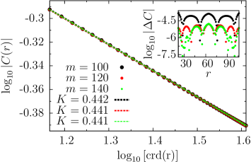
Figure 8: Hopping correlation functions $C(r)$ and fitted Luttinger parameters $K$ for three different bond dimensions $m$ in the clean case $\Delta=0$. The system size is $N_{s}=128$ and the interaction strength is $U=3.1$. The accuracy of $K$ is of the order of $10^{-3}$. The inset shows the difference $\Delta C$ between the data and the fitted lines.

Finally, in order to complement the data on the BKT transition in the clean system, we use the entanglement entropy (a quantity that is easily accessible by means of tensor network methods [17]) as an alternative criterion to locate the phase transition. To this end, we numerically calculate the von Neumann entropy $S(\ell)$ for various bipartitions $\ell\,|\,N_{s}-\ell$ of the ring. Since the SF phase is known to be critical (with central charge $c=1$), the entanglement entropy obeys [44]

$$S(\ell)=\frac{c}{3}\log\left[\mathrm{crd}(\ell)\right]+a\;,$$ (7)

with $a$ a non-universal constant. By fitting Eq. (7) ($a$ being the only free parameter) for different values of $U$, we expect to get an increase in the fit’s RMS error $\Delta_{\mathrm{RMS}}$ starting from $U_{c}$, where Eq. (7) is not valid any more because in the MI phase the von Neumann entropy $S(\ell)$ saturates for large $\ell$ (obeying an area law). As shown in Fig. 9, we find that the behavior of $\Delta_{\mathrm{RMS}}$ as a function of $U$ is well described by the form

$$\Delta_{\mathrm{RMS}}(U)=\cases{\Delta_{0}+\alpha\,\exp\left(-\frac{\gamma}{(U-U_{c})^{\beta}}\right)&for $U>U_{c}$\\ \Delta_{0}&for $U\leq U_{c}$\\ }\;,$$ (8)

which is closely related to the opening of the energy gap $E_{g}\sim\exp\left(-\delta/\sqrt{U-U_{c}}\right)$ at the BKT transition [45], with some constants $\Delta_{0}$, $\alpha$, $\beta$, $\gamma$, $\delta$. By fitting Eq. (8) to our data we obtain a numerical value of $U_{c}=3.26\pm 0.13$ for the transition point (equivalently, $t_{c}=0.306\pm 0.011$), see Fig. 9. Despite the fact that this result is compatible with the ones we obtained by means of the other methods, its precision is about one order of magnitude worse. This is due to the exponentially slow increase of $\Delta_{\mathrm{RMS}}$ in Eq. (8), which prevents a more accurate determination of $U_{c}$.

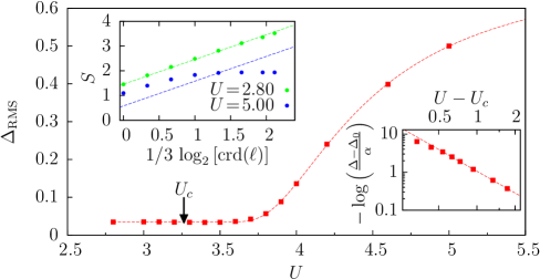
Figure 9: Determination of the BKT transition point by probing the scaling of the von Neumann entropy $S$ for a ring of $N_{s}=256$ sites without disorder ($\Delta=0$). After fitting Eq. (7) for various values of $U$ (see left inset for two examples, dashed lines are fits), the resulting RMS errors are used to determine $U_{c}$ via a fit of the form Eq. (8). Extracted fit parameters are $U_{c}=3.26\pm 0.13$, $\alpha=0.67\pm 0.04$, $\beta=1.9\pm 0.4$, $\gamma=1.1\pm 0.2$, $\Delta_{0}=0.035\pm 0.001$. The right inset shows the same data as the main panel, but scaled in such a way that the power-law inside the exponential of Eq. (8) becomes apparent.

In Tab. 1 we summarize the results for the SF-MI transition points $t_{c}$ obtained from the various techniques that we employed (superfluid density in Section 3, Luttinger parameter in Section 4, entanglement entropy). The mutual agreement of the obtained values is of the order of some $10^{-3}$.

Table 1: Comparison of the critical hopping strengths $t_{c}$ for the 1D Bose-Hubbard model without disorder, obtained from various numerical methods. Also shown are two values reported in earlier works [18, 46], see Refs. [50, 51, 52] for a comprehensive summary.

• Method	$t_{c}/U$
  Superfluid density	$0.295\pm 0.003$
  Luttinger parameter	$0.299\pm 0.002$
  Entanglement entropy	$0.306\pm 0.011$
  Kühner et al. [18]	$0.297\pm 0.010$
  Kashurnikov and Svistunov [46]	$0.304\pm 0.002$

Appendix B Convergence of distributions with respect to the number of disorder realizations

In Fig. 10 we demonstrate that the distributions of the Luttinger parameter $K$ can be meaningfully characterized with a number of disorder realizations of the order of $n_{r}=100$, even in the regime of relatively strong disorder $\Delta$. This statement holds true for all system sizes $N_{s}$ used in this work. Moreover, it becomes apparent that the distributions can be faithfully described by the log-normal distributions defined in Eq. (5). We remark that the identification of rare events with very large $K$, as described in [32, 35], would require system sizes and number of disorder realizations of the order of several thousand, which is not within the scope of the present investigation (see main text).

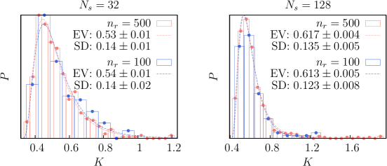
Figure 10: Distributions of the Luttinger parameter $K$ for two different system sizes $N_{s}$ and two different numbers of disorder realizations $n_{r}$. In both plots the disorder strength is $\Delta=3.0$ and the interaction is $U=2.2$. The characteristics of the distributions (in particular their expectation value (EV) and standard deviation (SD)) remain within the statistical error when increasing $n_{r}$ from $100$ to $500$. Fitted lines are log-normal distributions.

Appendix C Comparison of phase diagram with data from the literature

In this appendix we compare our data on the extension of the superfluid lobe (as summarized in Fig. 2) with results previously obtained in the literature, in particular with data from Prokof’ev et al. [26] and Rapsch et al. [27]. A direct comparison is shown in Fig. 11. As already mentioned in the main text, we observe good agreement with the Monte Carlo results reported in Ref. [26] (except for a slight deviation at the tip of the lobe).

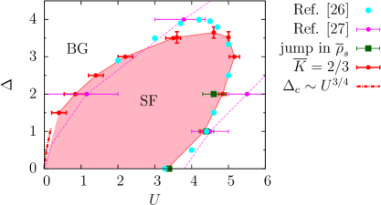
Figure 11: Comparison of the phase diagram from Fig. 2 with phase diagrams previously obtained in the literature.

Appendix D Local boson occupation numbers

In order to get an estimate for the necessary local (on-site) dimension $d$, one has to consider the expectation values $\langle n_{j}\rangle$ of the local boson number operators and their corresponding variances $\mathrm{Var}(n_{j})=\langle n_{j}^{2}\rangle-\langle n_{j}\rangle^{2}$. We plot these quantities in Fig. 12, both as a function of interaction strength $U$ (with disorder strength $\Delta$ fixed) and as a function of $\Delta$ ($U$ fixed). Adding two standard deviations to the highest occurring boson occupation expectation values along the ring, we find that up to $d=10$ states are relevant for the lowest $U$ values we simulated. By choosing $d=20$ for this regime (as reported in the main text) we can be absolutely sure that errors due to the truncation of the local boson bases are negligible. We can easily afford such high local dimensions $d$ because the impact on the computation time is relatively small in TTN simulations (e.g. for a $N_{s}=128$ simulation the runtime only increases by a factor of $1.3$ when using $d=20$ instead of $d=10$).

Furthermore, Fig. 12 suggests that for constant $U$ the maximally occurring occupation number increases linearly with the disorder strength $\Delta$.

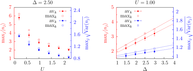
Figure 12: Local boson occupation expectation value and variance as a function of $U$ (left) and $\Delta$ (right). Red filled circles: realization-averaged maximally occurring expectation value $\mathrm{av}_{k}[\max_{j}\langle n_{j}\rangle]$ (indices $k$ and $j$ run over $n_{r}=100$ disorder realizations and $N_{s}=128$ sites, respectively). Red squares: highest measured expectation value $\max_{k}[\max_{j}\langle n_{j}\rangle]$. Blue filled circles: realization-averaged maximally occurring standard deviation $\mathrm{av}_{k}[\max_{j}\sqrt{\mathrm{Var}(n_{j})}]$. Blue squares: highest measured standard deviation $\max_{k}[\max_{j}\sqrt{\mathrm{Var}(n_{j})}]$. The plotted error bars are standard deviations determined from the realization ensembles. Dashed lines are linear fits.

References

References

- [1] M. P. A. Fisher, P. B. Weichman, G. Grinstein, and D. S. Fisher, Phys. Rev. B 40, 546 (1989).
- [2] M. P. A. Fisher, Phys. Rev. Lett. 65, 923 (1990).
- [3] R. Fazio and H. van der Zant, Phys. Rep. 355, 235 (2001).
- [4] A. Tomadin and R. Fazio, J. Opt. Soc. Am. B 27, A130 (2010).
- [5] D. Jaksch, C. Bruder, J. I. Cirac, C. W. Gardiner, and P. Zoller. Phys. Rev. Lett. 81, 3108 (1998).
- [6] M. Greiner, O. Mandel, T. Esslinger, T. W. Hänsch, and I. Bloch, Nature 415, 39 (2002).
- [7] M. Lewenstein, A. Sanpera, V. Ahufinger, B. Damski, A. Sen, and U. Sen, Adv. Phys. 56, 243 (2007).
- [8] I. Bloch, J. Dalibard, and W. Zwerger, Rev. Mod. Phys. 80, 885 (2008).
- [9] V. L. Berezinskii, Sov. Phys. JETP, 32, 493 (1971).
- [10] J. M. Kosterlitz and D. J. Thouless, Journal of Physics C Solid State Physics 6, 1181 (1973).
- [11] J. M. Kosterlitz, Journal of Physics C Solid State Physics 7, 1046 (1974).
- [12] D. R. Nelson and J. M. Kosterlitz, Phys. Rev. Lett. 39, 1201 (1977).
- [13] H. Weber and P. Minnhagen, Phys. Rev. B 37, 5986 (1988).
- [14] Y.-D. Hsieh, Y.-J. Kao, and A. W. Sandvik, JSTAT: Theory and Experiment, P09001 (2013).
- [15] G. G. Batrouni, R. T. Scalettar, and G. T. Zimanyi, Phys. Rev. Lett. 65, 1765 (1990).
- [16] M. A. Cazalilla, R. Citro, T. Giamarchi, E. Orignac, and M. Rigol, Rev. Mod. Phys. 83, 1405 (2011).
- [17] U. Schollwöck, Rev. Mod. Phys. 77, 259 (2005); Ann. Phys. 326, 96 (2011).
- [18] T. D. Kühner, S. R. White, and H. Monien, Phys. Rev. B 61, 12474 (2000).
- [19] M. Rizzi, D. Rossini, G. De Chiara, S. Montangero, and R. Fazio, Phys. Rev. Lett. 95, 240404 (2005).
- [20] P. Doria, T. Calarco, and S. Montangero, Phys. Rev. Lett. 106, 190501 (2011).
- [21] D. Rossini and R. Fazio, New J. Phys. 14, 065012 (2012).
- [22] Extensions of DMRG and MPS to treat systems with periodic boundary conditions have been discussed in P. Pippan, S. R. White, and H. G. Evertz, Phys. Rev. B 81, 081103(R) (2010); B. Pirvu, F. Verstraete and G. Vidal G, Phys. Rev. B 83, 125104 (2011); D. Rossini, V. Giovannetti, and R. Fazio, Phys. Rev. B 83, 140411(R) (2011).
- [23] T. Giamarchi and H. J. Schulz, Phys. Rev. B 37, 325 (1988).
- [24] R. V. Pai, R. Pandit, H. R. Krishnamurthy, and S. Ramasesha, Phys. Rev. Lett. 76, 2937 (1996).
- [25] I. F. Herbut, Phys. Rev. B 57, 13729 (1998).
- [26] N. V. Prokof’ev and B. V. Svistunov, Phys. Rev. Lett. 80, 4355 (1998).
- [27] S. Rapsch, U. Schollwöck, and W. Zwerger, EPL (Europhysics Letters) 46, 559 (1999).
- [28] L. Pollet, N. V. Prokof’ev, B. V. Svistunov, and M. Troyer, Phys. Rev. Lett. 103, 140402 (2009).
- [29] J. Carrasquilla, F. Becca, A. Trombettoni, and M. Fabrizio, Phys. Rev. B 81, 195129 (2010).
- [30] E. Altman, Y. Kafri, A. Polkovnikov, and G. Refael, Phys. Rev. Lett. 93, 150402 (2004).
- [31] S. Pielawa and E. Altman, Phys. Rev. B 88, 224201 (2013).
- [32] L. Pollet, N. V. Prokof’ev, and B. V. Svistunov, Phys. Rev. B 87, 144203 (2013).
- [33] Z. Ristivojevic, A. Petkovíc, P. Le Doussal, and T. Giamarchi, Phys. Rev. B 90, 125144 (2014).
- [34] A. M. Goldsborough and R. A. Römer, EPL (Europhysics Letters) 111, 26004 (2015).
- [35] L. Pollet, Comptes Rendus Physique 14, 712 (2013).
- [36] C. D’Errico, E. Lucioni, L. Tanzi, L. Gori, G. Roux, I. P. McCulloch, T. Giamarchi, M. Inguscio, and G. Modugno, Phys. Rev. Lett. 113, 095301 (2014).
- [37] Y.-Y. Shi, L.-M. Duan, and G. Vidal, Phys. Rev. A 74, 022320 (2006).
- [38] V. Murg, F. Verstraete, Ö. Legeza, and R. M. Noack, Phys. Rev. B 82, 205105 (2010).
- [39] P. Silvi, V. Giovannetti, S. Montangero, M. Rizzi, J. I. Cirac, and R. Fazio, Phys. Rev. A 81, 062335 (2010).
- [40] A. M. Goldsborough and R. A. Römer, Phys. Rev. B 89, 214203 (2014).
- [41] A. M. Goldsborough, S. A. Rautu, and R. A. Römer, Phys. Rev. E 91, 042133 (2015).
- [42] M. Gerster, P. Silvi, M. Rizzi, R. Fazio, T. Calarco, and S. Montangero, Phys. Rev. B 90, 125154 (2014).
- [43] S. Singh, R. N. C. Pfeifer, and G. Vidal, Phys. Rev. A 82, 050301(R) (2010).
- [44] P. Calabrese and J. Cardy, JSTAT: Theory and Experiment, P06002 (2004).
- [45] T. D. Kühner and H. Monien, Phys. Rev. B 58, 14741 (1998).
- [46] V. A. Kashurnikov and B. V. Svistunov, Phys. Rev. B 56, 11776 (1996).
- [47] T. Giamarchi and H. J. Schulz, EPL (Europhysics Letters) 3, 1287 (1987).
- [48] J. P. Álvarez Zúñiga, D. J. Luitz, G. Lemarié, and N. Laflorencie, Phys. Rev. Lett. 114, 155301 (2015).
- [49] L. Pollet, N. V. Prokof’ev, and B. V. Svistunov, Phys. Rev. B 89, 054204 (2014).
- [50] J. Carrasquilla, S. R. Manmana, and M. Rigol, Phys. Rev. A 87, 043606 (2013).
- [51] S. Rachel, N. Laflorencie, H. F. Song, and K. Le Hur, Phys. Rev. Lett. 108, 116401 (2012).
- [52] K. V. Krutitsky, Phys. Rep. 607, 1–101 (2016).
- [53] bwUniCluster: funded by the Ministry of Science, Research and Arts and the universities of the state of Baden-Württemberg, Germany, within the framework program bwHPC.