Routing in Unit Disk Graphs

Abstract

Let $S\subset\mathbb{R}^{2}$ be a set of $n$ sites. The unit disk graph $\operatorname{UD}(S)$ on $S$ has vertex set $S$ and an edge between two distinct sites $s,t\in S$ if and only if $s$ and $t$ have Euclidean distance $|st|\leq 1$.

A routing scheme $R$ for $\operatorname{UD}(S)$ assigns to each site $s\in S$ a label $\ell(s)$ and a routing table $\rho(s)$. For any two sites $s,t\in S$, the scheme $R$ must be able to route a packet from $s$ to $t$ in the following way: given a current site $r$ (initially, $r=s$), a header $h$ (initially empty), and the label $\ell(t)$ of the target, the scheme $R$ consults the routing table $\rho(r)$ to compute a neighbor $r^{\prime}$ of $r$, a new header $h^{\prime}$, and the label $\ell(t^{\prime})$ of an intermediate target $t^{\prime}$. (The label of the original target may be stored at the header $h^{\prime}$.) The packet is then routed to $r^{\prime}$, and the procedure is repeated until the packet reaches $t$. The resulting sequence of sites is called the routing path. The stretch of $R$ is the maximum ratio of the (Euclidean) length of the routing path produced by $R$ and the shortest path in $\operatorname{UD}(S)$, over all pairs of distinct sites in $S$.

For any given $\varepsilon>0$, we show how to construct a routing scheme for $\operatorname{UD}(S)$ with stretch $1+\varepsilon$ using labels of $O(\log n)$ bits and routing tables of $O(\varepsilon^{-5}\log^{2}n\log^{2}D)$ bits, where $D$ is the (Euclidean) diameter of $\operatorname{UD}(S)$. The header size is $O(\log n\log D)$ bits.

1 Introduction

Routing in graphs constitutes a fundamental problem in distributed graph algorithms [9, 15]. Given a graph $G$, we would like to be able to route a packet from any node in $G$ to any other node, where the destination node is represented by its label. The routing algorithm should be local, meaning that it uses only information stored with the packet and with the current node, and it should be efficient, meaning that the packet does not travel much longer than necessary. There is an obvious solution to this problem: with each node $s$ of $G$, we store the shortest path tree for $s$. Then it is easy to route a packet along the shortest path to its destination. However, this solution is very inefficient: we need to store the complete topology of $G$ with each node, leading to quadratic space usage. Thus, the goal of a routing scheme is to store as little information as possible with each node of the graph, such that we can still route a packet on a path of length close to shortest.

For general graphs a plethora of results is available, reflecting the work of almost three decades (see, e.g., [16, 3] and the references therein). However, for general graphs, any efficient routing scheme needs to store $\Omega(n^{\alpha})$ bits per node, for some $\alpha>0$ [15]. Thus, it is natural to ask whether improved results are possible for specialized graph classes. For example, for trees it is known how to obtain a routing scheme that follows a shortest path and requires $O(\log n)$ bits of information at each node [19, 7, 17]. In planar graphs, for any $\varepsilon>0$ it is possible to store a polylogarithmic number of bits at each node in order to route a packet along a path of length at most $1+\varepsilon$ times the length of the shortest path [18].

A graph class that is of particular interest for routing problems comes from the study of mobile and wireless networks. Such networks are traditionally modeled as unit disk graphs [4]. The nodes are represented by points in the plane, and two nodes are connected if and only if the distance between the corresponding points is at most one. Even though unit disk graphs may be dense, they share many properties with planar graphs, in particular with respect to algorithmic problems. There exists a vast literature on routing in unit disk graphs, developed in the wireless networking community (cf. [9]). Most of these schemes were designed with a different outlook, aiming at practical and simple solutions instead of provable worst-case guarantees. For example, the most popular routing method is called geographic routing. Here, we assume that the coordinates of the target site are known, and we route the packet to the neighbor that is closest to the target. Even though this is a good practical heuristic, it can happen that a packet gets stuck. There are several ways to modify geographic routing to obtain a routing scheme where a packet always reaches its target (if possible) [1, 11, 12]. However, in these schemes the routing path may be much longer than the shortest path.

To the best of our knowledge, the only compact routing scheme for unit disk graphs that achieves routing paths that are provably within a constant factor of the optimum is due to Yan, Xiang, and Dragan [20]. More precisely, they show how to assign a label of $O(\log^{2}n)$ bits to each node of the graph such that given the labels of a source $s$ and of a target $t$, one can compute a neighbor of $s$ that leads toward $t$. They prove that by repeating this procedure, one can obtain a path from $s$ to $t$ with at most $3d_{h}(s,t)+12$ hops, where $d_{h}(s,t)$ is the hop distance of $s$ and $t$. For this, Yan et al.extend a scheme by Gupta et al. [10] for planar graphs to unit disk graphs by using a delicate planarization argument to obtain small-sized balanced separators. Even though the scheme by Yan et al.is conceptually simple, it requires a detailed analysis with an extensive case distinction.

We propose an alternative approach to routing in unit disk graphs. Our scheme is based on the well-separated pair decomposition for unit disk graphs [8]. It stores a polylogarithmic number of bits at each node of the graph, and it constructs a routing path that can be made arbitrarily close to a shortest path, where the edges are weighted according to their Euclidean length (see Section 2 for a precise statement of our results). This compares favorably with the scheme by Yan et al. [20] which achieves only a constant factor approximation. Furthermore, our labels need only $O(\log n)$ bits and our scheme is arguably simpler to analyze. However, unlike the algorithm by Yan et al., our scheme requires that the packet contain a modifiable header with a polylogarithmic number of bits. It is an interesting open question whether a scheme with similar performance guarantees that does not require a modifiable header exists.

2 The Model and Our Results

Let $S\subset\mathbb{R}^{2}$ be a set of $n$ sites in the plane. We say that $S$ has density at most $\vartheta$ if every unit disk contains at most $\vartheta$ points from $S$. The density $\vartheta$ of $S$ is bounded if $\vartheta=O(1)$. The unit disk graph for $S$ is the graph $\operatorname{UD}(S)$ with vertex set $S$ and an edge $st$ between two distinct sites $s,t\in S$ if and only if $|st|\leq 1$, where $|\cdot|$ denotes the Euclidean distance. We define the weight of the edge $st$ to be its Euclidean length and use $d(\cdot,\cdot)$ to denote the shortest path distance in $\operatorname{UD}(S)$. Given a set $T\subset S$, we define $\operatorname{diam}(T)$ as the (Euclidean) diameter of the induced subgraph $\operatorname{UD}(T)$ of $\operatorname{UD}(S)$, i.e., the maximum length of a shortest path between two sites in $\operatorname{UD}(T)$.

We would like to compute a routing scheme for $\operatorname{UD}(S)$ with a small stretch and compact routing tables. Formally, a routing scheme for $\operatorname{UD}(S)$ consists of (i) a label $\ell(s)\in\{0,1\}^{*}$ and (ii) a routing table $\rho(s)\in\{0,1\}^{*}$, for each site $s\in S$. The labels and the routing tables correspond to a routing function $f:S\times\{0,1\}^{*}\times\{0,1\}^{*}\rightarrow S\times\{0,1\}^{*}\times\{0,1\}^{*}$. The function $f$ takes as input a current site $s$, the label $\ell(t)$ of a target site $t$, and a header $h\in\{0,1\}^{*}$. The routing function may use its input and the routing table $\rho(s)$ of $s$ to compute a new site $s^{\prime}$, a modified header $h^{\prime}$, and the label of an intermediate target $\ell(t^{\prime})$. The new site $s^{\prime}$ may be either $s$ or a neighbor of $s$ in $\operatorname{UD}(S)$. If $s^{\prime}=s$ then the packet stays at $s$ and we recompute the routing function at $s$ with the modified header and the label of the intermediate target. If $s^{\prime}$ is a neighbor of $s$ then $s$ sends the packet (with the header and the label of the intermediate target) to $s^{\prime}$. Even though the eventual goal of the packet is the target $t$, we introduce the intermediate target $t^{\prime}$ into the notation, since it allows for a more succinct presentation of the routing algorithm. (The original target can be stored with the modifiable header and will be extracted later according to the definition of the routing function. Similarly, the routing may proceed through several intermediate targets, but at each point in time, the routing function receives only one of them.)

Let $h_{0}$ be the empty header. For any two sites $s,t\in S$, consider the sequence of triples given by $(s_{0},\ell_{0},h_{0})=(s,\ell(t),h_{0})$ and $(s_{i},\ell_{i},h_{i})=f(s_{i-1},\ell_{i-1},h_{i-1})$ for $i\geq 1$. We say that the routing scheme is correct if for any two sites $s,t\in S$ there exists an index $k$ such that $s_{k}=t$.

We consider the minimal such index $k$, $k=k(s,t)\geq 0$ such that $s_{k}=t$ and $s_{i}\neq t$ for $i<k$. We say that the routing scheme reaches $t$ after $k$ steps. We call $s_{0},s_{1},\dots,s_{k}$ the routing path between $s$ and $t$, and we define the routing distance $d_{\rho}(s,t)$ between $s$ and $t$ as $d_{\rho}(s,t)=\sum_{i=1}^{k}|s_{i-1}s_{i}|$. Recall that $|\cdot|$ denotes the Euclidean distance.

The quality of the routing scheme is measured by several parameters:

• the label size $L(n)=\max_{|S|=n}\max_{s\in S}|\ell(s)|$,

• the table size $T(n)=\max_{|S|=n}\max_{s\in S}|\rho(s)|$,

• the header size $H(n)=\max_{|S|=n}\max_{s\neq t\in S}\max_{i=1,\dots,k(s,t)}|h_{i}|$,

• and the stretch $\varphi(n)=\max_{|S|=n}\max_{s\neq t\in S}\frac{d_{\rho}(s,t)}{d(s,t)}$.

We show that for any $S\subset\mathbb{R}^{2}$, $|S|=n$, and any $\varepsilon>0$ we can construct a routing scheme with $\varphi(n)=1+\varepsilon$, $L(n)=O(\log n)$, $T(n)=O(\varepsilon^{-5}\log^{2}n\log^{2}D)$, and $H(n)=O(\log n\log D)$, where $D=\operatorname{diam}(S)$ is the diameter of $\operatorname{UD}(S)$. We emphasize that in a unit disk graph, we always have $D\leq n$. We may also assume that $D\geq 2$: otherwise, $S$ could be approximated by an $\varepsilon$-net with $O(1)$ vertices, and we could route in $\operatorname{UD}(S)$ with routing tables and headers of constant size (see Section 5.4).

The high dependence on $1/\varepsilon$ renders our result mostly of theoretical interest. However, it demonstrates for the first time that the stretch can be made arbitrarily close to $1$ while maintaining routing tables of polylogarithmic size.

Even though our algorithm uses ideas from previous routing schemes, such as “interval routing” or hierarchical clustering [16], to the best of our knowledge, we are the first to use the well-separated pair decomposition [2] as the basis for a routing scheme. In general graphs, this approach is not possible, since in this metric, small well-separated pair decompositions do not exist [13]. As discussed above, in geometric settings, the focus has been on position-based methods that make stronger use of the geometry than the WSPD does [9]. Thus, our approach is more geometric than the traditional methods for general graphs, and at the same time more combinatorial than the methods based on geometry.

3 The Well-Separated Pair Decomposition for $\operatorname{UD}(S)$

Our routing scheme uses the well-separated pair decomposition (WSPD) for the unit disk graph metric given by Gao and Zhang [8]. WSPDs provide a compact way to efficiently encode the approximate pairwise distances in a metric space. Originally, WSPDs were introduced by Callahan and Kosaraju [2] in the context of the Euclidean metric, and they have found numerous applications since then (see e.g., [8, 14] and the references therein).

Since our routing scheme relies crucially on the specific structure of the WSPD described by Gao and Zhang, we remind the reader of the main steps of their algorithm and analysis.

First, Gao and Zhang assume that $S$ has bounded density and that $\operatorname{UD}(S)$ is connected. They construct the Euclidean minimum spanning tree $T$ for $S$. It is well known that $T$ is a spanning tree for $\operatorname{UD}(S)$ with maximum degree $6$. Furthermore, $T$ can be constructed in $O(n\log n)$ time [6]. Since $T$ has maximum degree $6$, there exists an edge $e$ in $T$ such that $T\setminus e$ consists of two trees with at least $\lceil(n-1)/6\rceil$ vertices each. By applying this observation recursively, we obtain a hierarchical decomposition $H$ of $T$. The decomposition $H$ is a binary tree. Each node $v$ of $H$ represents a subtree $T_{v}$ of $T$ with vertex set $S_{v}\subseteq S$ such that (i) the root of $H$ corresponds to $T$; (ii) the leaves of $H$ are in one-to-one correspondence with the sites in $S$; and (iii) let $v$ be an inner node of $H$ with children $u$ and $w$. Then $v$ has an associated edge $e_{v}\in T_{v}$ such that removing $e_{v}$ from $T_{v}$ yields the two subtrees $T_{u}$ and $T_{w}$ represented by $u$ and $w$. Furthermore, we have $|S_{u}|,|S_{w}|\geq\lceil(|S_{v}|-1)/6\rceil$.

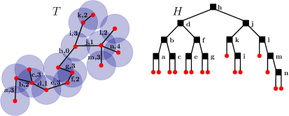
Figure 1: An EMST $T$ of $\operatorname{UD}(S)$ (left) where the edges are annotated with their level in the hierarchical decomposition $H$ (right).

It follows that $H$ has height $O(\log n)$. The depth $\delta(v)$ of a node $v\in H$ is defined as the number of edges on the path from $v$ to the root of $H$. The level of the associated edge $e_{v}$ of $v$ is the depth of $v$ in $H$. This uniquely defines a level for each edge in $T$. Now, for each node $v\in H$, the subtree $T_{v}$ is a connected component in the forest that is induced in $T$ by the edges of level at least $\delta(v)$ (see Figure 1).

After computing the hierarchical decomposition, the algorithm of Gao and Zhang essentially uses the greedy method of Callahan and Kosaraju [2] to construct a WSPD, with $H$ instead of the quadtree (or the fair split tree) in [2]. Let $c\geq 1$ be a separation parameter. The algorithm traverses $H$ and produces a sequence $\Xi=(u_{1},v_{1}),(u_{2},v_{2}),\dots,(u_{m},v_{m})$ of pairs of nodes of $H$, with the following properties:

1. The sets $S_{u_{1}}\times S_{v_{1}},S_{u_{2}}\times S_{v_{2}},\dots,S_{u_{m}}\times S_{v_{m}}$ constitute a partition of $S\times S$. This means that for each ordered pair of sites $(s,t)\in S\times S$, there is exactly one pair $(u,v)\in\Xi$ with $(s,t)\in S_{u}\times S_{v}$. We say that $(u,v)$ represents $(s,t)$.

2. Each pair $(u,v)\in\Xi$ is $c$-well-separated, i.e., we have

   $$(c+2)\max\{|S_{u}|-1,|S_{v}|-1\}\leq|\sigma(u)\sigma(v)|,$$ (1)

   where $\sigma(u),\sigma(v)$ are sites in $S_{u}$ and $S_{v}$, respectively, chosen by the algorithm. (This, in fact, holds for any pair of sites in $S_{u}$ and $S_{v}$, since the algorithm chooses $\sigma(u)$ and $\sigma(v)$ arbitrarily.)

Since in the shortest path metric of $\operatorname{UD}(S)$ the diameter $\operatorname{diam}(S_{u})$ is at most $|S_{u}|-1$ and since $|\sigma(u)\sigma(v)|\leq d(\sigma(u),\sigma(v))$, (1) implies that

$$(c+2)\max\{\operatorname{diam}(S_{u}),\operatorname{diam}(S_{v})\}\leq d(\sigma(u),\sigma(v)),$$ (2)

which is the traditional well-separation condition. However, (1) is easier to check algorithmically and has additional advantages that we will exploit in our routing scheme below.

Gao and Zhang show that their algorithm produces a $c$-WSPD with $m=O(\vartheta c^{2}n\log n)$ pairs, where $\vartheta$ is the density of $S$. More precisely, they prove the following lemma:

Lemma 3.1 (Lemma 4.3 and Corollary 4.6 in [8]).

For each node $u\in H$, the WSPD $\Xi$ has $O(\vartheta c^{2}|S_{u}|)$ pairs that contain $u$.∎

4 Preliminary Lemmas

We begin with two technical lemmas on WSPDs that will be useful later on. The first lemma shows that the choice of the sites $\sigma(u)$ for the nodes $u\in H$ is essentially arbitrary.

Lemma 4.1.

Let $\Xi$ be a $c$-WSPD for $S$ and let $s,t$ be two sites such that the pair $(u,v)\in\Xi$ represents $(s,t)$. Then $c\operatorname{diam}(S_{u})\leq c(|S_{u}|-1)\leq d(s,t)$.

Proof.

By triangle inequality and (1) we have

$$|st| \geq|\sigma(u)\sigma(v)|-2\max\{\operatorname{diam}(S_{u}),\operatorname{diam}(S_{v})\}$$

$$\geq(c+2)\max\{|S_{u}|-1,|S_{v}|-1\}-2\max\{\operatorname{diam}(S_{u}),\operatorname{diam}(S_{v})\}.$$

Since $|S_{u}|-1$ and $|S_{v}|-1$ are upper bounds for $\operatorname{diam}(S_{u})$ and $\operatorname{diam}(S_{v})$, respectively, and since $d(s,t)\geq|st|$, the claim follows. ∎

The next lemma shows that short distances are represented by singletons in the WSPD.

Lemma 4.2.

Let $\Xi$ be a $c$-WSPD for $S$ and let $s,t\in S$ be two sites with $d(s,t)<c$. If $(u,v)\in\Xi$ represents $(s,t)$, then $S_{u}=\{s\}$ and $S_{v}=\{t\}$.

Proof.

If $d(s,t)<c$, by Lemma 4.1 we have

$$c(|S_{u}|-1)\leq d(s,t)<c,$$

and thus $|S_{u}|<2$. The argument for $|S_{v}|$ is analogous. ∎

5 The Routing Scheme

Let $\vartheta$ be the density of $S$. First we describe a routing scheme whose parameters depend on $\vartheta$. Then we show how to remove this dependency and extend the scheme to work with arbitrary density. Our routing scheme uses the WSPD described in Section 3, and it is based on the following idea: let $\Xi$ be the $c$-WSPD for $\operatorname{UD}(S)$ and let $T$ be the EMST for $S$ used to compute it. We distribute the information about the pairs in $\Xi$ among the sites in $S$ (in a way to be described later) such that each site stores $O(\vartheta c^{2}\log n)$ pairs in its routing table.

To route from $s$ to $t$, we explore $T$, starting from $s$, until we find the site $r$ with the pair $(u,v)$ representing $(s,t)$. Our scheme will guarantee that $s$ and $r$ are sites in $S_{u}$, and therefore it suffices to walk along $T_{u}$ to find $r$ (see Figure 2). We call this first step in which we search for $(u,v)$ the local routing.

Together with the pair $(u,v)$, we store in $\rho(r)$ the middle site $m$ on the shortest path from $r$ to $\sigma(v)$, i.e., the vertex “halfway” between $r$ and $\sigma(v)$. Once we find $m$, we store $t$ at the header, and we recursively route the packet from $r$ to $m$. When the packet reaches $m$, we retrieve $t$ from the header and continue the routing from $m$ to $t$. To keep track of intermediate targets during the recursion, we store a stack of targets in the header. We call this second step that includes the recursive routing through the middle site, the global routing.

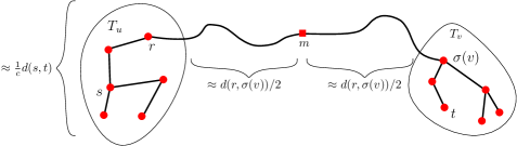
Figure 2: To route a packet from $s$ to $t$, we first walk along $T_{u}$ until we find $r$. Then we recursively route from $r$ to $m$ and from $m$ to $t$.

We now describe our routing scheme in detail. Let $1+\varepsilon$, $\varepsilon>0$, be the desired stretch factor.

5.1 Preprocessing

The preprocessing phase works as follows. We set $c=(\alpha/\varepsilon)\log D$, where $D=\operatorname{diam}(S)$ and $\alpha$ is a sufficiently large constant that we will fix later. Then we compute a $c$-WSPD for $\operatorname{UD}(S)$. As explained in Section 3, the WSPD consists of a bounded degree spanning tree $T$ of $\operatorname{UD}(S)$, a hierarchical balanced decomposition $H$ of $T$ whose nodes $u\in H$ correspond to subtrees $T_{u}$ of $T$, and a sequence $\Xi=(u_{1},v_{1}),(u_{2},v_{2}),\dots,(u_{k},v_{k})$ of $k=O(\vartheta c^{2}n\log n)=O(\vartheta\varepsilon^{-2}n\log n\log^{2}D)$ well-separated pairs that represent a partition of $S\times S$.

First, we determine the labeling $\ell$ for the sites in $S$. This is done as in the “interval routing scheme” of Santoro and Khatib [17] for trees. We perform a postorder traversal of $H$. Let $l$ be a counter which is initialized to $1$. Whenever we encounter a leaf of $H$, we set the label $\ell(s)$ of the corresponding site $s\in S$ to $l$, and we increment $l$ by $1$. Whenever we visit an internal node $u$ of $H$ for the last time, we annotate it with the interval $I_{u}$ of the labels in $T_{u}$. Thus, a site $s\in S$ lies in a subtree $T_{u}$ if and only if $\ell(s)\in I_{u}$. Each label has $O(\log n)$ bits.

Next, we describe the routing tables. Each routing table consists of two parts, the local routing table and the global routing table. The local routing table $\rho_{L}(s)$ of a site $s$ stores the neighbors of $s$ in $T$, in counterclockwise order, together with the levels in $H$ of the corresponding edges (cf. Section 3). Since $T$ has degree at most $6$, each local routing table consists of $O(\log n)$ bits.

The global routing table $\rho_{G}(s)$ of a site $s$ is obtained as follows: we go through all $O(\log n)$ nodes $u$ of $H$ that contain $s$ in their subtree $T_{u}$. By Lemma 3.1, $\Xi$ contains at most $O(\vartheta c^{2}|S_{u}|)$ well-separated pairs in which $u$ represents one of the sets. We assign $O(\vartheta c^{2})=O(\vartheta\varepsilon^{-2}\log^{2}D)$ of these pairs to $s$, such that each pair is assigned to exactly one site in $S_{u}$. For each pair $(u,v)$ assigned to $s$, we store the interval $I_{v}$ corresponding to $S_{v}$. Furthermore, if $\sigma(v)$ is not a neighbor of $s$, we store at $s$, together with the pair $(u,v)$, the label $\ell(m)$ of the middle site $m$ on a shortest path $\pi$ from $s$ to $\sigma(v)$. Formally, $m$ is a site on $\pi$ that minimizes the maximum distance, $\max\{d(s,m),d(m,\sigma(v))\}$, to the endpoints of $\pi$.

Lemma 5.1.

For every site $s$, $\rho_{G}(s)$ is of size $O(\vartheta\varepsilon^{-2}\log^{2}n\log^{2}D)$ bits.

Proof.

A site $s$ lies in $O(\log n)$ different sets $S_{u}$, at most one for each level of $H$. For each such set, we store $O(\vartheta\varepsilon^{-2}\log^{2}D)$ pairs in $\rho_{G}(s)$, each of which requires $O(\log n)$ bits. ∎

Finally, we argue that the routing scheme can be computed efficiently. Our preprocessing algorithm proceeds in a centralized fashion and processes the whole graph to determine the routing table for each node.

Lemma 5.2.

The preprocessing time for the routing scheme described above is $O(n^{2}\log n+\vartheta n^{2}+\vartheta\varepsilon^{-2}n\log n\log^{2}D)$.

Proof.

The $c$-WSPD can be computed in $O(\vartheta c^{2}n\log n)=O(\vartheta\varepsilon^{-2}n\log n\log^{2}D)$ time [8]. Within the same time bound, we can distribute the WSPD-pairs to the sites in $S$ and compute the labels for $S$.

It remains to compute the middle sites; we do this for all pairs $(s,t)\in S\times S$ as follows: we first compute $\operatorname{UD}(S)$ explicitly. Since $S$ has density $\vartheta$, we have $O(\vartheta n)$ edges in $\operatorname{UD}(S)$, and we can compute it naively in time $O(n^{2})$. For each $s\in S$, we compute the shortest path tree $\mathcal{T}$ with root $s$. This takes total time $O(n^{2}\log n+\vartheta n^{2})$, using $n$ invocations of Dijkstra’s algorithm.

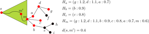
Figure 3: $m$ is the middle site for $g$ and $d$. $m^{\prime}$ is a better middle site for vertices at least as close to $m$ as $b$.

For each $s\in S$, we perform a post-order traversal of the shortest path tree $\mathcal{T}$ to find the middle sites for all $s$-$t$-paths. First, for each leaf $t$ of $\mathcal{T}$, we create a max-heap that contains $t$ with $d(s,t)$ as the key. We now describe how to process a site $m$ during the traversal. First, we merge the heaps of all children of $m$ into a new heap $H_{m}$ and we insert $m$ into $H$ with $d(s,m)$ as key, see Figure 3. During the traversal, we maintain the invariant that $H_{m}$ contains all sites that are descendants of $m$ in $\mathcal{T}$ for which we have not yet found a middle site. Furthermore, since $d(s,t)$ increases monotonically along every root-leaf path in $\mathcal{T}$, the sites for which $m$ might be the middle site are a prefix of the decreasingly sorted distances $d(s,t)$ with $t\in H$. Thus, to find the sites in $H_{m}$ for which $m$ is the middle site, we repeatedly perform an extract-max operation on $H_{m}$ to obtain the next candidate $t$. Then, we compare the value of $\max\{d(s,m),d(m,t)\}$ with $\max\{d(s,m^{\prime}),d(m^{\prime},t)\}$, where $m^{\prime}$ is the parent of $m$ in $\mathcal{T}$. That is, we check if $m^{\prime}$ is a “better” middle site than $m$. If not, $m$ must be the middle site for $s$-$t$. Otherwise, $m$ cannot be the middle site for any other site in $H_{m}$, and we proceed with our traversal. Using, e.g., Fibonacci Heaps, we can merge two heaps in $O(1)$ time and perform an extract-max operation in $O(\log n)$ amortized time [5]. Since each element of $\mathcal{T}$ is inserted and extracted at most once, we need $O(n\log n)$ time to find the middle sites for $s$. Thus, we can find all middle sites in time $O(n^{2}\log n)$ and the total preprocessing time is $O(n^{2}\log n+\vartheta n^{2}+\vartheta\varepsilon^{-2}n\log n\log^{2}D)$. ∎

5.2 Routing a Packet

Suppose we are given two sites $s$ and $t$, and we would like to route a packet from $s$ to $t$. Recall our overall strategy: we first perform a local exploration of $\operatorname{UD}(S)$ in order to discover a site $r$ that stores a pair $(u,v)\in\Xi$ representing $(s,t)$ in its global routing table $\rho_{G}(r)$. To find $r$, we consider the subtrees of $T$ that contain $s$ by increasing size, and we perform an Euler tour in each subtree until we find $r$. In $\rho_{G}(r)$ we have stored the middle site $m$ of a shortest path from $r$ to $\sigma(v)$. We put $t$ into the header, and we recursively route the packet from $r$ to $m$. Once we reach $m$, we retrieve the original target $t$ from the header and recursively route from $m$ to $t$, see Algorithm 1 for pseudo-code.

Local Routing: The Euler-Tour.

We start at $s$, and we would like to find the site $r$ that stores the pair $(u,v)$ representing $(s,t)$. By construction, both $s$ and $r$ are contained in $S_{u}$, and it suffices to perform an Euler tour on $T_{u}$ to discover $r$. Since we do not know $u$ in advance, we begin with the parent of the leaf in $H$ that contains $s$, and we explore all nodes on the path to the root until we find $u$ (see Figure 4).

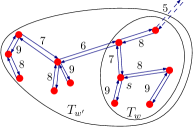
Figure 4: To find $r$ we do an Euler Tour on $T_{w}$, the subtree that contains $s$ whose edges have level at least $7$. Since we do not find $r$, we search the next larger subtree $T_{w^{\prime}}$, where $w^{\prime}$ is the parent of $w$ in $H$ by decreasing the search level to $6$.

Let $w\in H$ be the node to be explored, and let $l=\delta(w)$ be the depth of $w$ in $H$. The header $h$ contains $l$, the current level being explored, and $e$, the (directed) start edge. The start edge $e$ is the unique edge of level $\delta(s)-1$ incident to $s$, i.e., the edge associated with the parent of $s$ in $H$. Recall that $T_{w}$ is a connected component of the forest induced by all edges of level at least $l$. We perform an Euler tour on $T_{w}$ using the local routing tables.

To begin the tour, we follow the start edge $e$ from $s$. This edge is contained in all non-trivial subtrees containing $s$. Throughout the search, we maintain in the header the previous vertex before the current vertex, i.e., when we reach a vertex $r$ through the edge $(r^{\prime},r)$, the header contains the previous vertex $r^{\prime}$.

Every time we visit a site $r$, we check for all WSPD-pairs $(u,v)$ in $\rho_{G}(r)$ whether $\ell(t)\in I_{v}$, i.e., whether $t\in S_{v}$. If so, we clear the local routing information from $h$, and we proceed with the global routing. If not, we retrieve from the header the vertex $r^{\prime}$ through which we just arrived to $r$ and we scan $\rho_{L}(r)$ to find the first edge $(r,r^{\prime\prime})$ of level at least $l$ in clockwise order after $(r,r^{\prime})$, going back to the beginning of $\rho_{L}(r)$ if necessary. If the edge $(r,r^{\prime\prime})$ is different from the start edge $e$, then $(r,r^{\prime\prime})$ is next edge of the Euler tour. We remember $r$ as the previous vertex in the header, and we proceed to $r^{\prime\prime}$. Otherwise, if $(r,r^{\prime\prime})=e$, the Euler tour of $T_{w}$ tries to traverse the start edge for a second time. This means that $T_{w}$ does not contain the desired middle site. We decrease $l$ by one, and we again follow the start edge. Decreasing $l$ corresponds to proceeding to the parent of $w$ in $H$ and hence to the next larger subtree.

Global Routing: The WSPD.

Suppose we are at a site $s$ such that $\rho_{G}(s)$ contains the pair $(u,v)$ with the target $t$ being in $S_{v}$. If $t$ is not a neighbor of $s$, then $\rho_{G}(s)$ must contain the label of a middle site $m$ for $(u,v)$. We push (the label of) $t$ onto the header stack, we set $m$ to be the new target and we apply the routing function again (with $\ell(m)$ and the new header). If $t$ is a neighbor of $s$, we go directly to $t$ without changing the target and the header.

When we reach the current destination and the stack at the header is not empty then we pop the next target from the header and apply the routing function again. Otherwise, the current destination is the final one and the routing is complete.

Input: currentSite $s$, targetLabel $\ell(t)$, header $h$

Output: nextSite, nextTargetLabel, header

1 if $\ell(s)=\ell(t)$ then /* intermediate target reached? */

2       if $h.\textnormal{stack}=\emptyset$ then /* final target? */

3             return $(s,\perp,\perp)$

4      else

5             return $(s,h.\text{stack.pop}(),h)$

6else if $\rho(s)$ stores a WSPD-pair $(u,v)$ with $t\in S_{v}$ then /* global routing */

7       $h.\text{startEdge}\leftarrow\emptyset$

8       if $s\textnormal{ and }t\textnormal{ are neighbors in }\operatorname{UD}(S)$ then

9             return $(t,\ell(t),h)$

10      else

11             $\text{nextTargetLabel}\leftarrow\text{label of middle site for }(u,v)$

12             $h.\text{stack.push}(\ell(t))$

13             return $(s,\text{nextTargetLabel},h)$

14else  /* local routing */

15       if h.startEdge $=\emptyset$ then /* initialize local routing */

16             $h.\text{level}\leftarrow\delta(s)-1$

17             $r\leftarrow$ neighbor of $s$ with level of edge $sr=h.\text{level}$

18             $h.\text{startEdge}\leftarrow sr$

19            

20      else

21             $r\leftarrow$ clockwise neighbor of $s$ following $h.\text{prevVertex}$ with level of $sr\geq h.\text{level}$

22             if $sr=h.\text{startEdge}$ then /* Euler tour has finished tree */

                   $h.\text{level}\leftarrow h.\text{level}-1$

                    /* try next level */

23                  

24      $h.\text{prevVertex}\leftarrow s$

25       return $(r,\ell(t),h)$

Algorithm 1 The routing function. In the resutling triple the source is either the current vertex $s$, in which case we apply the routing function again at $s$, or it is a neighbor $s^{\prime}$ of $s$, in which case the packet is sent to $s^{\prime}$.

5.3 Analysis of the Routing Scheme

We now prove that the described routing scheme is correct and has low stretch, i.e., that for any two sites $s$ and $t$, it produces a routing path $s=s_{0},\dots,s_{k}=t$ of length at most $(1+\varepsilon)d(s,t)$.

5.3.1 Correctness

We now prove that our scheme is correct. For small distances, the routing path is actually optimal.

Lemma 5.3.

Let $s,t$ be two sites in $S$. Then, the routing scheme produces a routing path $s_{0},s_{1},\dots,s_{k}$ with the following properties

1. $s_{0}=s$ and $s_{k}=t$,

2. the header stack is in the same state at the beginning and at the end of the routing path, and

3. if $d(s,t)<c$, then $d_{\rho}(s,t)=d(s,t)$.

Proof.

We prove that our routing scheme has properties (i)–(iii) by induction on the rank of $d(s,t)$ in the sorted list of the pairwise distances in $\operatorname{UD}(S)$.

For the base case, consider the edges $st$ in $\operatorname{UD}(G)$, i.e., $d(s,t)=|st|\leq 1$. By Lemma 4.2, there exists a pair $(u,v)\in\Xi$ with $S_{u}=\{s\}$ and $S_{v}=\{t\}$. Thus, Algorithm 1 correctly routes to $t$ in one step. It uses a shortest path and does not manipulate the header stack. All properties are fulfilled.

Next, consider an arbitrary pair $s,t$ with $1<d(s,t)<c$. By Lemma 4.2, there is a pair $(u,v)\in\Xi$ with $S_{u}=\{s\}$ and $S_{v}=\{t\}$. By construction, $(u,v)$ is stored in $\rho_{G}(s)$ and the routing algorithm directly proceeds to the global routing phase. Since $d(s,t)>1$, the routing table contains a middle site $m$ and since $S_{u}$ and $S_{v}$ are singletons, $m$ is a middle site on a shortest path from $s$ to $t$. Algorithm 1 pushes $\ell(t)$ onto the stack and sets $m$ as the new target. By induction, the routing scheme now routes the packet along a shortest path from $s$ to $m$ (items i and iii of the induction hypothesis), and when the packet arrives at $m$, the target label $\ell(t)$ is at the top of the stack (item ii). Thus, Algorithm 1 executes line 1, and routes the packet from $m$ to $t$. Again by induction, the packet now follows a shortest path from $m$ to $t$ (i, iii), and when the packet arrives at $t$, the stack is in the same state a before pushing $\ell(t)$ (ii). The claim follows.

Finally, consider an arbitrary pair $s,t\in S$ such that $d(s,t)\geq c$. By construction, our routing scheme will eventually find a site $r\in S$ whose global routing table stores a WSPD-pair $(u,v)$ that represents $(s,t)$. Up to the point in which we reach $r$ the stack remains unchanged (see Figure 5). If $\sigma(v)$ is a neighbor of $r$ then by Lemma 4.1, $|S_{u}|=|S_{v}|=1$. So $\sigma(v)=t$ and the packet arrives to $t$ from $r$ in a single step with the header in its original state. Otherwise, there is a middle site $m$ associated with $(u,v)$ in $\rho(r)$.

Algorithm 1 pushes $\ell(t)$ onto the stack and sets $m$ as the new target. By induction, the routing scheme routes the packet correctly from $s$ to $m$ (i), and when the packet arrives at $m$, the target label $\ell(t)$ is at the top of the stack (ii). Thus, Algorithm 1 executes line 1, and routes the packet from $m$ to $t$. Again by induction, the packet arrives at $t$, with the stack in the same state as before pushing $\ell(t)$ (i, ii). ∎

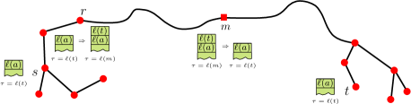
Figure 5: How the stack (green) and the target label $\tau$ change due to the global routing.

5.3.2 Stretch factor

The analysis of the stretch factor requires some more technical work. We begin with a lemma that justifies the term “middle site”.

Lemma 5.4.

Let $s,t$ be two sites in $S$ with $d(s,t)\geq c\geq 13$ and let $(u,v)\in\Xi$ be the WSPD-pair that represents $(s,t)$. If $m$ is a middle site of a shortest path from $s$ to $\sigma(v)$ in $\operatorname{UD}(S)$, then

1. $d(s,m)+d(m,t)\leq\left(1+\frac{2}{c}\right)d(s,t)$, and

2. $d(s,m),d(m,t)\leq\frac{5}{8}d(s,t)$.

Proof.

For (i) we have

$$d(s,m)+d(m,t) \leq d(s,m)+d(m,\sigma(v))+d(\sigma(v),t)$$ (triangle inequality)

$$=d(s,\sigma(v))+d(\sigma(v),t) m$$ ( is middle site)

$$\leq d(s,t)+2d(\sigma(v),t)$$ (triangle inequality)

$$\leq\left(1+\frac{2}{c}\right)d(s,t),$$ (Lemma 4.1)

where the last inequality also uses the fact that $d(\sigma(v),t)\leq\operatorname{diam}(S_{v})$.

For (ii) let $\pi$ be a shortest path from $s$ to $\sigma(v)$ that contains $m$, and let $m^{\prime}$ be the point on $\pi$ with distance $d(s,\sigma(v))/2$ from $s$ and from $\sigma(v)$ ($m^{\prime}$ may lie on an edge of $\pi$). Since the edges of $\pi$ have length at most $1$ and since $m$ is the middle site, we have $d(m,m^{\prime})=|mm^{\prime}|\leq 1/2$. Hence,

$$\max\{d(s,m),d(m,\sigma(v))\}\leq\frac{d(s,\sigma(v))}{2}+\frac{1}{2}.$$ (3)

Using triangle inequality and Lemma 4.1 we get

$$\left(1-\frac{1}{c}\right)d(m,t)\leq d(m,\sigma(v))$$ (4)

and

$$d(s,\sigma(v))\leq\left(1+\frac{1}{c}\right)d(s,t).$$ (5)

Using (3), (4), and (5) we can derive

$$\max\{d(s,m),d(m,t)\} \leq\left(1+\frac{1}{c-1}\right)\max\{d(s,m),d(m,\sigma(v))\}$$ (by (4))

$$\leq\left(1+\frac{1}{c-1}\right)\left(\frac{d(s,\sigma(v))}{2}+\frac{1}{2}\right)$$ (by (3))

$$\leq\left(1+\frac{1}{c-1}\right)\left(\left(1+\frac{1}{c}\right)\frac{d(s,t)}{2}+\frac{1}{2}\right)$$ (by (5))

$$\leq\left(1+\frac{1}{c-1}\right)\left(1+\frac{2}{c}\right)\frac{d(s,t)}{2}$$ (*)

$$\leq\left(\frac{1}{2}+\frac{3}{2c-2}\right)d(s,t),$$

where (*) is due to the assumption that $d(s,t)\geq c$. Now (ii) follows from the assumption that $c\geq 13$. ∎

In the next lemma, we bound the distance traveled during the local routing.

Lemma 5.5.

Let $s,t$ be two sites in $S$ with $d(s,t)\geq c$. Then, the total distance traveled by the packet during the local routing phase before the WSPD-pair representing $(s,t)$ is discovered, is at most $(48/c)d(s,t)$.

Proof.

Let $(u,v)$ be the WSPD-pair representing $(s,t)$, and let $u_{0},u_{1},\dots,u_{k}=u$ be the path in $H$ from the leaf $u_{0}$ of $s$ to $u$. Let $T_{0},T_{1},\dots,T_{k}$ and $S_{0},S_{1},\dots,S_{k}$ be the corresponding subtrees of $T$ and sites of $S$. The local routing algorithm iteratively performs an Euler tour of $T_{0},T_{1},\dots,T_{k}$ (the tour of $T_{k}$ may stop early). An Euler tour in $T_{i}$ takes $2|S_{i}|-2$ steps, and each edge has length at most $1$. As described in Section 3, for $i=0.\dots,k-1$, the WSPD ensures that

$$|S_{i}|\leq|S_{i+1}|-\left\lceil\frac{|S_{i+1}|-1}{6}\right\rceil\leq\frac{5}{6}\,|S_{i+1}|+\frac{1}{6}\leq\frac{11}{12}\,|S_{i+1}|,$$

since $|S_{i+1}|\geq 2$. It follows that the total distance for the local routing is at most

$$\sum_{i=0}^{k}(2|S_{i}|-2)\leq 2|S_{k}|\sum_{i=0}^{k}\left(\frac{11}{12}\right)^{i}\leq 24|S_{k}|.$$

By Lemma 4.1, we have $d(s,t)\geq c(|S_{u}|-1)$ and since $S_{k}=S_{u}$ the total distance is bounded by $24|S_{u}|\leq 24(d(s,t)/c+1)\leq(48/c)d(s,t)$, where the last inequality is true for $d(s,t)\geq c$. ∎

Finally, we can bound the stretch factor as follows.

Lemma 5.6.

For any two sites $s$ and $t$, we have $d_{\rho}(s,t)\leq\bigl{(}1+\varepsilon)d(s,t)$.

Proof.

We show by induction on $d_{\rho}(s,t)$ that there is an $\alpha>0$ with

$$d_{\rho}(s,t)\leq\left(1+\frac{\alpha}{c}\,\log d(s,t)\right)d(s,t).$$

Since $d(s,t)\leq\operatorname{diam}(S)=D$, the lemma then follows from our choice of $c=(\alpha/\varepsilon)\log D$.

If $d(s,t)<c$, the claim follows by Lemma 5.3(iii): the packet is routed along a shortest path and incurs no detour. If $d(s,t)\geq c$, Algorithm 1 performs a local routing to find the site $r$ that has the WSPD-pair $(u,v)$ representing $(s,t)$ stored in $\rho_{G}(r)$. Then the packet is routed recursively from $r$ to the middle site $m$ and from $m$ to $t$. By Lemma 5.5 the length of the routing path is $d_{\rho}(s,t)\leq(48/c)d(s,t)+d_{\rho}(r,m)+d_{\rho}(m,t)$, and by induction we get

$$d_{\rho}(s,t) \leq\frac{48}{c}\,d(s,t)+\left(1+\frac{\alpha}{c}\,\log d(r,m)\right)d(r,m)+\left(1+\frac{\alpha}{c}\,\log d(m,t)\right)d(m,t).$$

Since $$m r \sigma(v) \operatorname{UD}(S) \log(5/8)\leq-1/2$$ is a middle site on a shortest --path in , Lemma 5.4(i),(ii) and the fact that imply

$$d_{\rho}(s,t) \leq\frac{48}{c}d(s,t)+\left(1+\frac{\alpha}{c}\,\log(d(r,t))-\frac{\alpha}{2c}\right)\left(1+\frac{2}{c}\right)d(r,t).$$

By the triangle inequality we have $d(r,t)\leq d(s,t)+\operatorname{diam}(S_{u})$, so Lemma 4.1 gives

$$d_{\rho}(s,t) \leq\frac{48}{c}\,d(s,t)+\left(1+\frac{\alpha}{c}\log\left(\left(1+\frac{1}{c}\right)d(s,t)\right)-\frac{\alpha}{2c}\right)\left(1+\frac{2}{c}\right)\left(1+\frac{1}{c}\right)d(s,t)$$

$$\leq\frac{48}{c}\,d(s,t)+\left(1+\frac{\alpha}{c}\log\left(\left(1+\frac{1}{c}\right)d(s,t)\right)-\frac{\alpha}{2c}\right)\left(1+\frac{4}{c}\right)d(s,t),$$

for $c$ large enough. For $\alpha>192$, we can eliminate the first term to get

$$d_{\rho}(s,t) \leq\left(1+\frac{\alpha}{c}\log\left(\left(1+\frac{1}{c}\right)d(s,t)\right)-\frac{\alpha}{4c}\right)\left(1+\frac{4}{c}\right)d(s,t),$$

and since now $$c\geq 192 \log(1+1/c)\leq 1/8$$ and hence ,

$$d_{\rho}(s,t) \leq\left(1+\frac{\alpha}{c}\log(d(s,t))-\frac{\alpha}{8c}\right)\left(1+\frac{4}{c}\right)d(s,t)=\left(1+\frac{\alpha}{c}\log d(s,t)\right)d(s,t)+\Delta,$$

with

$$\Delta=-\frac{\alpha}{8c}\,\left(1+\frac{4}{c}\right)d(s,t)+\frac{4}{c}\,d(s,t)\left(1+\frac{\alpha}{c}\,\log d(s,t)\right).$$

It remains to show that $\Delta\leq 0$, i.e., that

$$\frac{4}{c}d(s,t)\left(1+\frac{\alpha}{c}\,\log d(s,t)\right)\leq\frac{\alpha}{8c}\,\left(1+\frac{4}{c}\right)d(s,t).$$

Now, since we picked $c=(\alpha/\varepsilon)\log D$ and $\alpha\geq 192$, we have

$$1+\frac{\alpha}{c}\,\log(d(s,t))\leq 2\leq\frac{\alpha}{32}\left(1+\frac{4}{c}\right),$$

as desired. This finishes the proof. ∎

Combining Lemma 5.1, Lemma 5.2, and Lemma 5.6 we obtain the following theorem.

Theorem 5.7.

Let $S$ be a set of $n$ sites in the plane with density $\vartheta$. For any $\varepsilon>0$, we can preprocess $S$ into a routing scheme for $\operatorname{UD}(S)$ with labels of size $O(\log n)$ bits and routing tables of size $O(\vartheta\varepsilon^{-2}\log^{2}n\log^{2}D)$ bits, where $D$ is the diameter of $\operatorname{UD}(S)$. For any two sites $s$,$t$, the scheme produces a routing path with $d_{\rho}(s,t)\leq(1+\varepsilon)d(s,t)$ and during the routing the maximum header size is $O(\log n\log D)$. The preprocessing time is $O(n^{2}\log n+\vartheta n^{2}+\vartheta\varepsilon^{-2}n\log n\log^{2}D)$.

5.4 Extension to Arbitrary Density

Let $1+\varepsilon$, $\varepsilon>0$, be the desired stretch factor. To extend the routing scheme to point sets of unbounded density, we follow a strategy similar to Gao and Zhang [8, Section 4.2]: we first pick an appropriate $\varepsilon_{1}>0$, and we compute an $\varepsilon_{1}$-net $R\subseteq S$, i.e., a subset $R$ of sites such that each site in $S$ has distance at most $\varepsilon_{1}$ to the closest site in $R$ and such that any two sites in $R$ are at distance at least $\varepsilon_{1}$ from each other, see Figure 6.

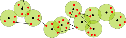
Figure 6: The set $R$ (black) and the bridges (endpoints of black edges) form the set $Z$.

As we show below, it is easy to see that $R$ has density $O(\varepsilon_{1}^{-2})$, and we would like to represent each site in $S$ by the closest site in $R$. However, the connected components of $\operatorname{UD}(R)$ might differ from those of $\operatorname{UD}(S)$. To rectify this, we add additional sites to $R$. This is done as follows: two sites $s,t\in R$ are called neighbors if $|st|>1$, but there are $p,q\in S$ such that $s,p,q,t$ is a path in $\operatorname{UD}(S)$ and such that $|sp|\leq\varepsilon_{1}$ and $|qt|\leq\varepsilon_{1}$ (possibly, $s=p$ or $q=t$). In this case, the pair of sites $p$ and $q$ is called a bridge for $s,t$. Let $R^{\prime}$ be a point set that contains an arbitrary bridge for each pair of neighbors in $R$. Set $Z=R\cup R^{\prime}$. The following simple volume argument shows that $Z$ has density $\vartheta=O(\varepsilon_{1}^{-3})$.

Lemma 5.8.

The set $R$ has density $O(\varepsilon_{1}^{-2})$ and the set $Z$ has density $O(\varepsilon_{1}^{-3})$.

Proof.

Let $D$ be a unit disk and let $D^{\prime}$ be the disk with radius $1+\varepsilon_{1}/2$ concentric to $D$. For each $s\in R\cap D$, the disk $D(s,\varepsilon_{1}/2)$ with center $s$ and radius $\varepsilon_{1}/2$ is contained in $D^{\prime}$. Let $s,t\in R$ be two sites. By construction $|st|\geq\varepsilon_{1}$ and thus the disks $D(s,\varepsilon_{1}/2)$ and $D(t,\varepsilon_{1}/2)$ are disjoint. A disk of radius $\varepsilon_{1}/2$ has area $\pi\varepsilon_{1}^{2}/4$ and the area of $D^{\prime}$ is $\pi(1+\varepsilon_{1}/2)^{2}$. Thus we can place $O(\varepsilon_{1}^{-2})$ such disks into $D^{\prime}$ disjointly. Hence, the density of $R$ is $O(\varepsilon_{1}^{-2})$.

Now, let $D^{\prime\prime}$ be the disk with radius $1+\varepsilon_{1}$ concentric to $D$. To bound the density of $Z$, let $p\in(Z\setminus R)\cap D$ be a site that belongs to a bridge. Suppose that $s\in R$ is responsible for $p$ being a bridge site. Then we have $|sp|\leq\varepsilon_{1}$ and by construction $s\in D^{\prime\prime}$. We charge $p$ to $s$. The same volume argument as above shows that $|R\cap D^{\prime\prime}|=O(1/\varepsilon_{1}^{-2})$. Below we show that $s$ has $O(\varepsilon_{1}^{-1})$ neighbors and thus can get $O(\varepsilon_{1}^{-1})$ charges from bridge sites. Hence, the number of bridge sites in $Z\cap D$, and also the density of $Z$, is $O(\varepsilon_{1}^{-3})$.

Consider the annulus $A$ around $s$ with inner radius $1$ and outer radius $1+2\varepsilon_{1}$. All neighbors of $s$ must lie in $A$. Let $A^{\prime}$ the annulus concentric to $A$ with inner radius $1-\varepsilon_{1}/2$ and outer radius $1+(5/2)\varepsilon_{1}$. The area of $A^{\prime}$ is

$$\pi\left(1+\frac{5}{2}\varepsilon_{1}\right)^{2}-\pi\left(1-\frac{\varepsilon_{1}}{2}\right)^{2}=6\varepsilon_{1}+6\varepsilon_{1}^{2},$$

and thus, since $R$ is an $\varepsilon_{1}$-net, we can place $O(\varepsilon_{1}^{-1})$ sites of $R$ in $A$. Hence, $s$ has $O(\varepsilon_{1}^{-1})$ neighbors, as claimed. ∎

Furthermore, Gao and Zhang show the following:

Lemma 5.9 (Lemma 4.8 and Lemma 4.9 in [8]).

We can compute $Z$ in $O((n/\varepsilon_{1}^{2})\log n)$ time, and if $d^{Z}(\cdot,\cdot)$ denotes the shortest path distance in $\operatorname{UD}(Z)$, then, for any $s,t\in R$, we have $d^{Z}(s,t)\leq(1+12\varepsilon_{1})d(s,t)+12\varepsilon_{1}$.

Now, our extended routing scheme proceeds as follows: first, we compute $R$ and $Z$ as described above, and we perform the preprocessing algorithm for $Z$ with $\varepsilon_{1}$ as the stretch parameter. We assign arbitrary new labels to the sites in $S\setminus Z$. Then, we extend the label $\ell(s)$ of each site $s\in S$, such that it also contains the label of a site in $R$ closest to $s$. The label size remains $O(\log n)$.

To route between two sites $s,t\in S$, we first check whether we can go from $s$ to $t$ in one step (we assume that this can be checked locally by the routing function). If so, we route the packet directly. Otherwise, we have $d(s,t)>1$. Let $s^{\prime},t^{\prime}\in R$ be the closest sites in $R$ to $s$ and to $t$. By construction, we can obtain $s^{\prime}$ and $t^{\prime}$ from $\ell(s)$ and $\ell(t)$. Now, we first go from $s$ to $s^{\prime}$. Then, we use the low-density algorithm to route from $s^{\prime}$ to $t^{\prime}$ in $\operatorname{UD}(Z)$, and finally we go from $t^{\prime}$ to $t$ in one step. Using the discussion above, the total routing distance is bounded by

$$d_{\rho}(s,t) \leq|ss^{\prime}|+d^{Z}_{\rho}(s^{\prime},t^{\prime})+|t^{\prime}t|,$$

where $$d^{Z}_{\rho}(\cdot,\cdot) \operatorname{UD}(Z)$$ is the routing distance in . By Lemma 5.6 and 5.9, this is

$$\leq\varepsilon_{1}+(1+\varepsilon_{1})d^{Z}(s^{\prime},t^{\prime})+\varepsilon_{1}$$

$$\leq 2\varepsilon_{1}+(1+\varepsilon_{1})\bigl{(}(1+12\varepsilon_{1})d(s^{\prime},t^{\prime})+12\varepsilon_{1}\bigr{)},$$

and by using the triangle inequality twice this is

$$\leq 2\varepsilon_{1}+(1+\varepsilon_{1})\bigl{(}(1+12\varepsilon_{1})(d(s,t)+2\varepsilon_{1})+12\varepsilon_{1}\bigr{)}.$$

Rearranging and using $$d(s,t)>1$$ yields

$$\leq(1+29\varepsilon_{1}+50\varepsilon_{1}^{2}+24\varepsilon_{1}^{3})d(s,t)\leq(1+\varepsilon)d(s,t),$$

where the last inequality holds for $\varepsilon_{1}\leq\varepsilon/103$. This establishes our main theorem:

Theorem 5.10.

Let $S$ be a set of $n$ sites in the plane. For any $\varepsilon>0$, we can preprocess $S$ into a routing scheme for $\operatorname{UD}(S)$ with labels of $O(\log n)$ bits and routing tables of size $O(\varepsilon^{-5}\log^{2}n\log^{2}D)$, where $D$ is the diameter of $\operatorname{UD}(S)$. For any two sites $s$,$t$, the scheme produces a routing path with $d_{\rho}(s,t)\leq(1+\varepsilon)d(s,t)$ and during the routing the maximum header size is $O(\log n\log D)$. The preprocessing time is $O(n^{2}\log n+\varepsilon^{-3}n^{2}+\varepsilon^{-5}n\log n\log^{2}D)$.

Proof.

The theorem follows from the above discussion and from the fact that the set $Z$ has density $O(\varepsilon^{-3})$, by our choice of $\varepsilon_{1}$. ∎

6 Conclusion

We have presented an efficient routing scheme for unit disk graphs that produces a routing path whose length can be made arbitrarily close to optimal. For this, we used the fact that the unit disk graph metric admits a small WSPD. Our techniques almost solely rely on properties of well-separated pairs and thus we expect our approach to generalize to other graph metrics for which WSPDs can be found. One such example is the hop-distance $d_{h}(\cdot,\cdot)$ in unit disk graphs, in which all edges have length $1$. Let $S$ be a set of sites and let $\operatorname{diam}_{h}(S)$ denote the diameter of $S$ in terms of $d_{h}(\cdot,\cdot)$. Since $\operatorname{diam}_{h}(S)\leq|S|-1$ and $|st|\leq d_{h}(s,t)$ for every two sites $s,t\in S$, the well-separation condition (1) implies also separation with respect to the hop-distance. Thus, we can also find a routing scheme that approximates the number of hops used in the routing path instead of its Euclidean length.

Various open questions remain. First of all, it would be interesting to improve the size of the routing tables. One way to achieve this might be to decrease the dependency on $\varepsilon$. The $\varepsilon^{-5}$-factor seems to be rather high. It is mostly due to the $\varepsilon^{-3}$-factor that we introduced in Section 5.4 when extending the routing scheme to a set of sites of unbounded density. Further improvements might be on the side of the WSPD: traditional WSPDs have only $O(c^{2}n)$ pairs, while the WSPD of Gao and Zhang has an additional logarithmic factor. Whether this factor can be avoided is still an open question and any improvement in the number of pairs would immediately decrease the size of our routing tables by the same amount.

Furthermore, our routing scheme makes extensive use of a modifiable header. While this is coherent with the usual model for routing schemes, the scheme of Yan et al. does not need such a header. In order to be completely comparable to their result, we would need to have a routing scheme that only requires a small routing table to produce a routing path with stretch $1+\varepsilon$.

References

- [1] P. Bose, P. Morin, I. Stojmenovic, and J. Urrutia. Routing with guaranteed delivery in ad hoc wireless networks. Wireless Networks, 7(6):609–616, 2001.
- [2] P. Callahan and S. Kosaraju. A decomposition of multidimensional point sets with applications to -nearest-neighbors and -body potential fields. J. ACM, 42(1):67–90, 1995.
- [3] S. Chechik. Compact routing schemes with improved stretch. In Proc. 32nd ACM Symp. on Principles of Distributed Computing (PODC), pages 33–41, 2013.
- [4] B. N. Clark, C. J. Colbourn, and D. S. Johnson. Unit disk graphs. Discrete Math., 86(1–3):165–177, 1990.
- [5] T. H. Cormen, C. E. Leiserson, R. L. Rivest, and C. Stein. Introduction to Algorithms. MIT Press, third edition, 2009.
- [6] M. de Berg, O. Cheong, M. van Kreveld, and M. Overmars. Computational Geometry: Algorithms and Applications. Springer, 3rd edition, 2008.
- [7] P. Fraigniaud and C. Gavoille. Routing in trees. In Proc. 28th Internat. Colloq. Automata Lang. Program. (ICALP), pages 757–772, 2001.
- [8] J. Gao and L. Zhang. Well-separated pair decomposition for the unit-disk graph metric and its applications. SIAM J. Comput., 35(1):151–169, 2005.
- [9] S. Giordano and I. Stojmenovic. Position based routing algorithms for ad hoc networks: A taxonomy. In Ad Hoc Wireless Networking, pages 103–136. Springer, 2004.
- [10] A. Gupta, A. Kumar, and R. Rastogi. Traveling with a Pez dispenser (or, routing issues in MPLS). SIAM J. Comput., 34(2):453–474, 2004.
- [11] B. Karp and H. T. Kung. GPSR: greedy perimeter stateless routing for wireless networks. In Proc.6th Annual Int. Conf. Mobile Computing and Networking (MOBICOM), pages 243–254, 2000.
- [12] F. Kuhn, R. Wattenhofer, Y. Zhang, and A. Zollinger. Geometric ad-hoc routing: of theory and practice. In Proc.22nd ACM Symp. Principles Dist. Comp. (PODC), pages 63–72, 2003.
- [13] J. S. B. Mitchell and W. Mulzer. Proximity algorithms. In C. Toth, J. O’Rourke, and J. Goodman, editors, Handbook of Discrete and Computational Geometry. CRC Press, third edition, 2017. to appear.
- [14] G. Narasimhan and M. H. M. Smid. Geometric spanner networks. Cambridge University Press, 2007.
- [15] D. Peleg and E. Upfal. A trade-off between space and efficiency for routing tables. J. ACM, 36(3):510–530, 1989.
- [16] L. Roditty and R. Tov. New routing techniques and their applications. In Proc. 34th ACM Symp. on Principles of Distributed Computing (PODC), pages 23–32, 2015.
- [17] N. Santoro and R. Khatib. Labelling and implicit routing in networks. Comput. J., 28(1):5–8, 1985.
- [18] M. Thorup. Compact oracles for reachability and approximate distances in planar digraphs. J. ACM, 51(6):993–1024, 2004.
- [19] M. Thorup and U. Zwick. Compact routing schemes. In Proc. 13th ACM Symposium on Parallel Algorithms and Architectures (SPAA), pages 1–10, 2001.
- [20] C. Yan, Y. Xiang, and F. F. Dragan. Compact and low delay routing labeling scheme for unit disk graphs. Comput. Geom., 45(7):305–325, 2012.