Particle-in-Cell Codes for plasma-based particle acceleration

Abstract

Basic principles of particle-in-cell (PIC ) codes with the main application for plasma-based acceleration are discussed. The ab initio full electromagnetic relativistic PIC codes provide the most reliable description of plasmas. Their properties are considered in detail. Representing the most fundamental model, the full PIC codes are computationally expensive. The plasma-based acceleration is a multi-scale problem with very disparate scales. The smallest scale is the laser or plasma wavelength (from one to hundred microns) and the largest scale is the acceleration distance (from a few centimeters to meters or even kilometers). The Lorentz-boost technique allows to reduce the scale disparity at the costs of complicating the simulations and causing unphysical numerical instabilities in the code. Another possibility is to use the quasi-static approximation where the disparate scales are separated analytically.

1 Introduction

Plasma-based particle acceleration involves a rather nonlinear medium, the relativistic plasmas [1]. This medium requires proper numerical simulation tools. During the past decades, Particle-in-Cell (PIC) methods have been proven to be a very reliable and successful method of kinetic plasma simulations [2, 3, 4, 5]. This success of PIC codes relies to a large extent on the very suggestive analogy with the actual plasma. The plasma in reality is an ensemble of many individual particles, electrons and ions, interacting with each other by the self-consistently generated fields. The PIC code is very similar to that, with the difference that number of the numerical particles, or macroparticles we follow in the code, may be significantly smaller. One may think as if one numerical “macroparticle” is a clump, or cloud, of many real particles, which occupy a finite volume in space and all move together with the same velocity. The consequent conclusion is that we have a “numerical plasma” consisting of heavy macroparticles, which have the same charge-to-mass ratio as the real plasma electrons and ions, but substitute many of those.

Depending on the application, different approximations can be chosen. The most fundamental approximation is the full electromagnetic PIC codes solving the Maxwell equations together with the relativistic equations of motion for the numerical particles. These “ab initio“ simulations produce the most detailed results, but can be also very expensive. In the case of long scale acceleration, when the driver propagates distances many times larger than its own length, the quasi-static approximation can be exploited. In this case, it is assumed that the driver changes little as it propagates distance comparable with its own length. The quasi-statics allows for separation of fast and slow variables and great acceleration of the simulation at the cost of radiation: the laser pulse or any emitted radiation cannot be described directly by such codes. Rather, a an additional module for the laser pulse is required, usually in the envelope approximation.

In this work, we describe the basic principles of the PIC methods, both full electromagnetic and quasi-static in application to plasma-based acceleration.

2 The basic equations

First, let us formulate the problem we are going to solve. We are doing electromagnetic and kinetic simulations. This means, we are solving the full set of Maxwell equations [6]

$$\frac{\partial{\bf E}}{\partial t} = c\nabla\times{\bf B}-4\pi{\bf j},$$ (1)

$$\frac{\partial{\bf B}}{\partial t} = -c\nabla\times{\bf E},$$ (2)

$$\nabla\cdot{\bf E} = 4\pi\rho,$$ (3)

$$\nabla\cdot{\bf B} = 0,$$ (4)

where we use CGS units and $c$ is the speed of light in vacuum.

Let us stop for a moment at this very fundamental system of equations. The electric and magnetic fields, ${\bf E,B}$, evolve according to the time-dependent equations (1)-(2) with the source term in the form of current density ${\bf j}$. This current is produced by the self-consistent charge motion in our system of particles. It is well known from the textbooks on electrodynamics (see, e.g., [6]), that the Gauss law (3) together with the curl-free part of Eq. (2), lead to the charge continuity equation

$$\frac{\partial\rho}{\partial t}+\nabla\cdot{\bf j}=0.$$ (5)

One can apply the operator $\nabla\cdot$ to the Faraday law (2) and use the Gauss Eq. (3) for $\nabla\cdot{\bf E}$, to obtain (5). The opposite is true as well. If the charge density always satisfies the continuity Eq. (5), the Gauss Eq. (5) is fulfilled automatically during evolution of the system, if it was satisfied initially. The symmetric consideration is valid for the magnetic field ${\bf B}$. As there is no magnetic charges, Eq. (4) remains always valid, if it was valid initially.

This means, we may reduce our problem to a solution of the two evolutionary equations (1)-(2) considering Eqs. (3),(4) as initial conditions only. This appears to be a very important and fruitful approach. PIC codes using it have a “local” algorithm, i.e., at each time step the information is exchanged between neighboring grid cells only. No global information exchange is possible because the Maxwell equations have “absolute future” and “absolute past” [7]. This property make the corresponding PIC codes perfectly suitable for parallelizing and, in addition, the influence (of always unphysical) boundary conditions is strongly reduced.

3 Kinetics and hydrodynamics

Now we have to define our source term, ${\bf j}$. In general, for this purpose, we have to know the distribution function of plasma particles

$$F^{N}({\bf x_{1},p_{1},...,x_{N},p_{N}}).$$ (6)

It defines the probability of an $N-$particles system to take a particular configuration in the $6N-$dimensional phase space. Here ${\bf x_{n},p_{n}}$ are coordinates and momenta of the $n$-th particle. The function (6) provides the exhaustive description of the system. However, as it is shown in statistical physics (see, e.g., [8]), single-particle distribution function for each species of particles may be sufficient to describe the full system. The sufficient condition is that the inter-particle correlations are small, and can be treated perturbatively. The equation, which governs the evolution of the single-particle distribution function $f({\bf x,p})$ is called Boltzmann-Vlasov Eq. [9, 10]:

$$\frac{\partial f}{\partial{t}}+\frac{{\bf p}}{m\gamma}\nabla f+\frac{{\bf F}}{m}\nabla_{p}f=St,$$ (7)

where $m$ is the single-particle mass of the corresponding species, $\gamma=\sqrt{1+(p/mc)^{2}}$ is the relativistic factor, ${\bf F}$ is the force, and $St$ is the collisional term (inter-particle correlations).

The kinetic equation (7) on the single-particle distribution function is $6-$dimensional and still complicated. It is a challenge to solve it analytically or numerically.

It appears, however, that under appropriate conditions one can make further simplifications. It is shown in statistics, that inter-particle collisions lead to the Maxwellian distribution function ($H-$theorem, see, e.g., [8]). In the non-relativistic case the Maxwellian distribution has the form:

$$f({\bf{x,v})=\frac{n({\bf x)}}{\sqrt{2\pi T}}e^{-\frac{({\bf v-V})^{2}}{2mT}},}$$ (8)

where $n({\bf x})$ is the local particle density, $T$ is the temperature, and ${\bf V}$ is the local streaming velocity. The characteristic time for establishing of the Maxwellian distribution is the inter-particle collision time.

Thus, if the effective collisional time in the considered system is short in comparison with other characteristic times, the distribution function remains Maxwellian. It is sufficient then to write evolutionary equations on the momenta of the distribution function, such as the local density

$$n({\bf x})=\int\,f({\bf x,v})\,d^{3}v{\bf}$$ (9)

the hydrodynamic velocity

$${\bf V}({\bf x})=\int\,{\bf v}f({\bf x,v})\,{\bf dv}{\bf,}$$ (10)

and the temperature

$$T({\bf x})=\int\,\frac{({\bf v-V})^{2}}{2m}f({\bf x,v})\,d^{3}v{\bf,}$$ (11)

are called fluid-like, or of hydrodynamic type.

4 Vlasov and Particle-in-Cell codes

If, however, the distribution function does deviate, or is expected to deviate significantly from the Maxwellian one, we have to solve the Boltzmann-Vlasov Eq. (7). What could be the appropriate numerical approach here?

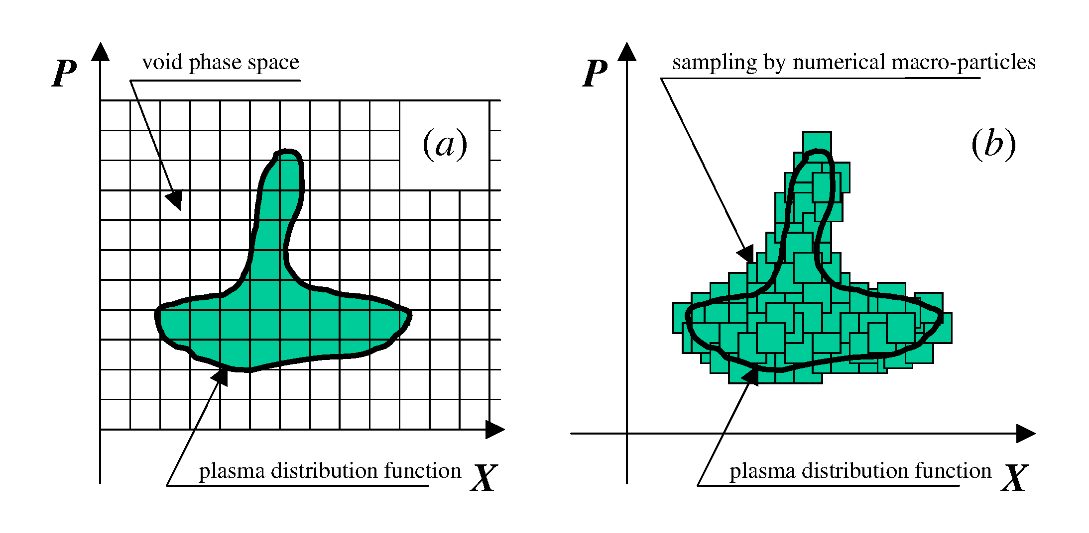
Figure 1: Kinetic plasma simulations. (a) Vlasov method: Eulerian grid in the phase space; (b) PIC method: numerical macroparticles mark the distribution function.

At the first look, it seems that the most straightforward and relatively simple approach is to solve the partial differential Eq. (7) using finite differences on the Eulerian grid in phase space. Indeed, this approach is pursued by several groups [11], and gains even more popularity as the power of available computers grows. One of the potential advantages of these Vlasov codes is the possibility of producing “smooth” results. Indeed, the Vlasov codes handle the distribution function, which is a smoothly changing real number already giving the probability to find the plasma particles in the corresponding point of the phase space.

The Vlasov codes, however, are very expensive from the computational point of view, and even one-dimensional problems may demand the use of parallel super-computers. The reason, why these codes need so much computational power, becomes clear from Fig. 1a. It shows schematically a mesh one would need for a ${\bf 1d1v}$ Vlasov code. The notation ${\bf 1d1v}$ means, that the code resolves one spatial coordinate and one coordinate in the momentum (velocity) space. The dashed region is to represent the part of the phase space occupied by plasma particles, where the associated $2-$dimensional distribution function $f(x,p_{x})$ is essentially non-zero. The unshaded region is empty from particles, and nothing interesting happens there. Nevertheless, one has to maintain these empty regions as parts of the numerical arrays, and process them when solving Eq. (7) on the Eulerian grid. This processing of empty regions leads to enormous wasting of computational power. This decisive drawback becomes even bolder with increase in the dimensionality of the problem under consideration. The efficiency of Vlasov codes drops exponentially with the number of dimensions, and becomes miniscule in the real ${\bf 3d3v}$ case, when one has to maintain in the memory and process a $6-$dimensional mesh, most of it just empty from particles.

Now let us show that there is another, presently more computationally effective, method to solve the Boltzmann-Vlasov Eq. (7). This is the finite-element method. The principle is illustrated in Fig. 1b. Again, imagine some distribution function in the phase space (the shaded region). Now, let us approximate, or sample, this distribution function by a set of Finite Phase-Fluid Elements (FPFE):

$$f({\bf x,p})=\sum_{n}~{}W_{n}^{ph}~{}S^{ph}({\bf x-x}_{n},{\bf p-p}_{n})$$ (12)

where $W_{n}^{ph}$ is the “weight” of the FPFE, and $S^{ph}({\bf x,p})$ is the “phase shape”, or the support function in the phase space. The center of the FPFE is positioned at ${\bf x}_{n},~{}{\bf p}_{n}$. We are free to make a particular choice of the support function. For simplicity, we choose here a ${\bf 6d}$ hypercube:

$$S^{ph}({\bf x},{\bf p})=1,~{}~{}|x_{\alpha}|<\frac{\Delta x_{\alpha}}{2},~{}~{}|p_{\alpha}|<\frac{\Delta p_{\alpha}}{2},~{}~{}\alpha=x,y,z$$

where $\Delta x_{\alpha}$ is the FPFE size along the $j-$axis in configuration space, and $\Delta p_{\alpha}$ is the FPFE size along the $p_{\alpha}-$axis in momenta space.

The “phase fluid” transports the distribution function along the characteristics of the Boltzmann-Vlasov Eq. (7) (see, e.g., [18]). Thus, we have to advance the centers of FPFE along the characteristics:

$$\frac{d{\bf x}_{n}}{dt} = \frac{{\bf p}}{m\gamma},$$ (13)

$$\frac{d{\bf p}_{n}}{dt} = {\bf F+F_{st}},$$ (14)

where ${\bf F_{st}}$ is the effective “collisional” force due to the collisional term in Eq. (7). The FPFE follow the evolution of distribution function in the phase space. Of course, the Eqs. (13)-(14) are the relativistic equations of motion of particles! Thus, the FPFE method is equivalent to the PIC method.

The significant advantage of the finite element method over the Vlasov codes is that one does not need to maintain a grid in the full phase space. Instead, our FPFE sample (or mark) only the interesting regions, where particles are present, and something important is going on. We still do maintain a grid in the configuration space to solve the field equations (1)-(2), but this grid has only 3 (and not 6 as in the Vlasov case) dimensions. Thus, PIC codes may be considered as “packed”, or “Lagrangian” Vlasov codes. Moreover, the finite phase fluid element approach is even more fundamental than the Boltzmann-Vlasov equation itself, because it may be easily generalized to the case when one macroparticle corresponds to just one real particle, and when inter-particle correlations are not small. The corresponding codes are usually called P³M: particle-particle-particle-mesh codes [5].

As soon as we consider our macroparticles not as simply “large clumps of real particles”, but as finite elements in the phase space, we discover, that there is no fundamental obstacle to the simulation of a cold plasma. Moreover, it is in this case where the finite elements approach becomes effective computationally and superior to the Vlasov codes. The phase space of a cold plasma is degenerate. The particles occupy a mere $3-$dimensional hypersurface of the full $6-$dimensional phase space. Evidently, this hypersurface can be accurately sampled even by a relatively small number of macroparticles (FPFE). As the system evolves, this surface deforms, stretches and contracts, but remains degenerate and three-dimensional, unless any heating (diffusion in the phase space) is present. There is a full stock of interesting physical phenomena in relativistic laser-plasma interactions one would like to study, where the physical collisional heating is negligible. Unfortunately, the numerical heating present in the “standard” PIC codes [4] leads to an unphysical numerical diffusion in the phase space, which spoils the picture. The code able to simulate initially cold plasma must be energy conservative.

5 Continuity equation

Historically, the first particle-in-cell codes were electrostatic [5], and they have to solve explicitly the Poisson equation

$$\nabla^{2}\phi=-4\pi\rho,$$ (15)

giving the static electric field

$${\bf E}_{\parallel}=-\nabla\phi.$$ (16)

The way of generalization to the electromagnetic case seemed quite natural. One simply adds the vector-potential ${\bf A}$:

$${\bf E}={\bf E}_{\parallel}+{\bf E}_{\perp}=-\nabla\phi-\frac{1}{c}\frac{\partial{\bf A}}{\partial t}.$$ (17)

Yet, there is another way of treating the electromagnetic fields. We have established in the previous section, that the simultaneous solution of Ampere’s law (1) and the continuity equation (5) satisfies the Gauss law (3) automatically. Thus, one may work with the fields ${\bf E}$ and ${\bf B}$ directly, not introducing the electrostatic potential $\phi$, and not solving the Poisson equation (15).

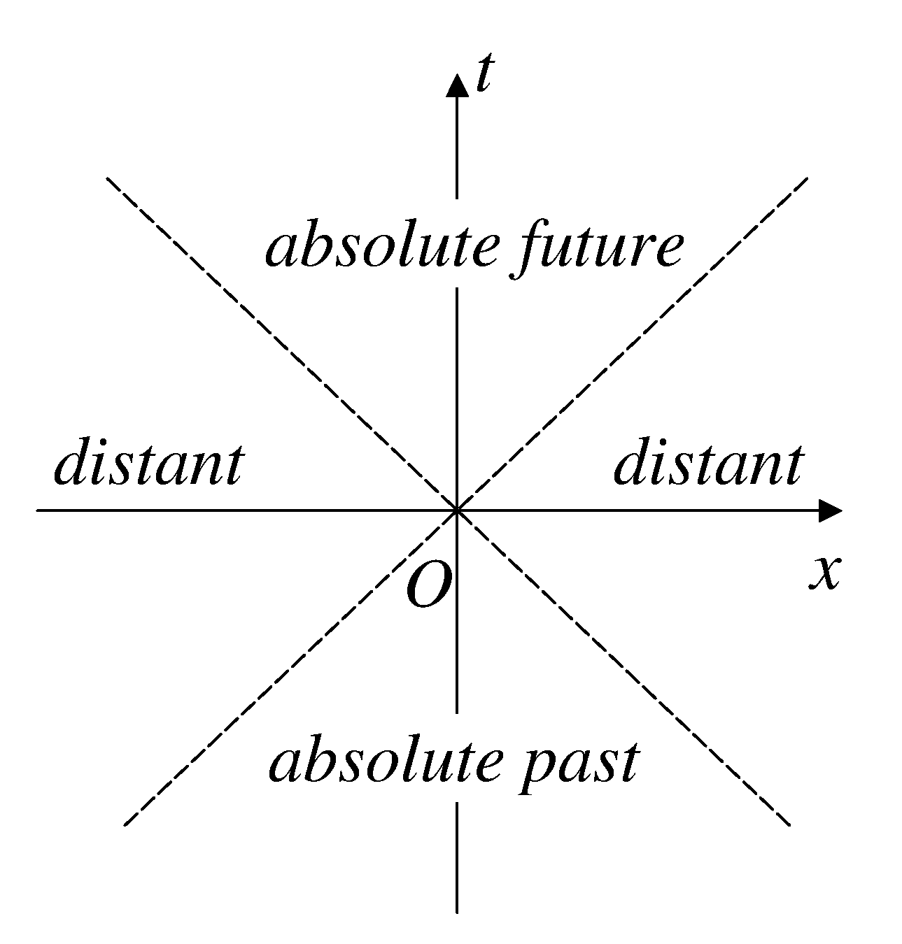
Figure 2: Minkovski space-time diagram illustrating the causality in the special relativity theory.

It is very advantageous to avoid solution of the Poisson equation (15), as it is nonlocal. This is an elliptical equation, and its solution essentially depends on the (usually unphysical) boundary conditions. A small perturbation or numerical error at the boundary may cause a global perturbation in the full simulation domain. In contrast, the Maxwell equations (1), (2) are local. Any signal can propagate no faster than the vacuum speed of light, and we apply here the Minkovsky diagram, Fig. 2. As the central event $(t_{n},x_{i},y_{j},z_{k})$, we choose some grid cell with the indices $(n,i,j,k)$ so that $t_{n}=n*\tau$, $x_{i}=i*\Delta x$, $y_{j}=j*\Delta y$, $z_{k}=k*\Delta z$. Here we denote $\tau,\Delta x,\Delta y,\Delta z$ the numerical steps on time, $X-$, $Y-$ and $Z-$axises. The light cone separates the full 4-dimensional space into the regions of the “absolute past”, the “absolute future”, and the region of “absolutely distant” events. Only the events taking place in the “absolute past” may stay in a casual connection with the central event. Thus, fields at the grid position $(t_{n},x_{i},y_{j},z_{k})$ are influenced by the events happening at the time moment $t_{n-1}$ at the grid cells located within the circle $c\tau$ around the original cell. If we use an explicit numerical scheme, then the time step is limited through the Courant condition, $c\tau<\min(\Delta x,\Delta y,\Delta z)$, and only the first neighboring cells are involved. A numerical scheme that does have this physical property is called local. In this sense, any numerical scheme that involves the solution of an elliptical equation like the Poisson one (15), is non-local.

It appears, that the key issue for the development of a local numerical scheme is the method of current deposition on the grid during the particle motion. Let us consider the cubic FPFE (numerical particle) on a grid. We suppose, that the particle and the grid elementary volume (the cell volume) $V_{c}=\Delta x\Delta y\Delta z$ are identical. So that the particle size length $\Delta x_{\alpha}$ is also the grid step along $\alpha-$axis, $\alpha=x,y,z$. We mark further the grid cells with the indexes $i,j,k$ along the axises $x,y,z$.

Figure 3: Yee lattice.

In the discussion of multi-dimensional PIC codes, we normally use the staggered or Yee lattice (grid), as illustrated in Fig. 3. We define the charge density on the grid at the centers of the cells, $\rho_{i+1/2,j+1/2,k+1/2}$, we get:

$$\rho_{i+1/2,j+1/2,k+1/2}=\sum_{n}~{}W_{n}^{\rho}~{}S^{\rho}({\bf x_{i+1/2,j+1/2,k+1/2}-x}_{n}).$$ (18)

The charge density interpolation weight and form of the particle are

$$S^{\rho}({\bf x}) = S_{x}^{\rho}(x)S_{y}^{\rho}(y)S_{z}^{\rho}(z),$$

$$S_{j}^{\rho}({\bf x_{j}}) = 1-2\frac{|x_{j}|}{\Delta_{j}}$$

$$|x_{j}|<0.5\Delta_{j}.$$

The scheme (5) is the “volume” (or “area”) weighting. It actually assigns the part of the particle residing in a cell to the cell’s center.

Now, if the particle moves, it generates current. How should one interpolate the current to the grid cells? One may try to use a straightforward interpolation, say, ${\bf J}=\sum_{n}{\bf V_{n}}S_{n}^{\rho}$, or others discussed in detail in Birdsall & Langdon book [4]. Quite naturally, these voluntary interpolations do not satisfy the continuity equation, i.e., the current flux through a cell boundaries defined in this way does not represent the actual charge change in the cell. The further consequence of this procedure appears when we integrate in time the Ampere law (1). The obtained electric field just does not satisfy the Gauss law (3).

One of the possible solutions of this inconsistency is to correct the obtained electric field [4]. Suppose, we have advanced the electric field ${\bf E^{\prime}}$ according to (1), and we got difficulties with the Gauss law: $\nabla\cdot{\bf E^{\prime}}\neq 4\pi\rho$. We may try to correct the electric field. We introduce a potential $\delta\phi$, such that

$$\nabla^{2}\delta\phi=-4\pi\rho+{\bf E^{\prime}},$$ (20)

and construct the corrected electric field

$${\bf E}={\bf E}-\nabla\delta\phi,$$ (21)

which does satisfy the Gauss law:

$$\nabla{\bf E}=4\pi\rho.$$ (22)

Unfortunately, this correction requires a solution of the nonlocal elliptical problem (20).

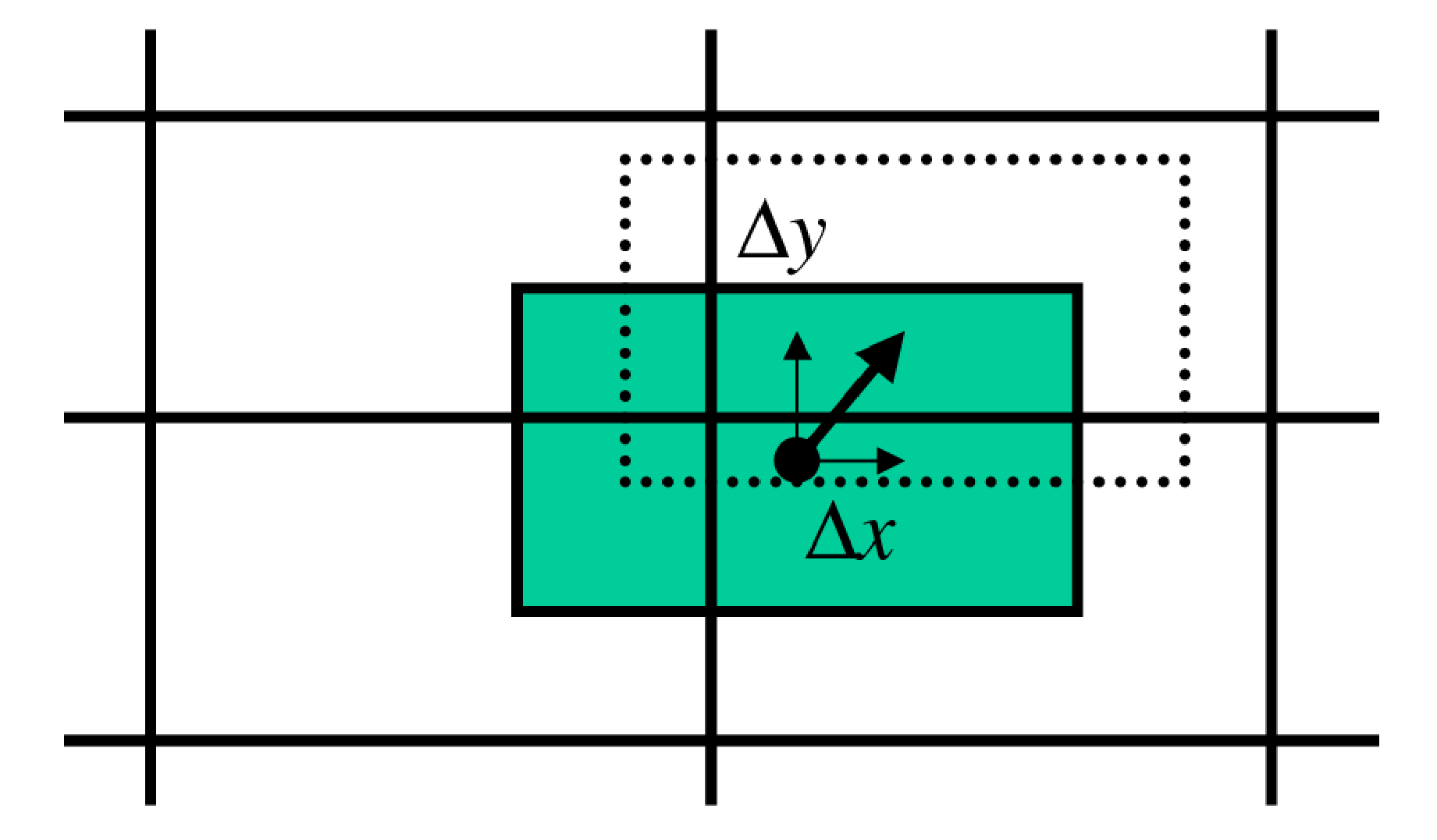
Figure 4: Tracing of particle trajectory

It appears, however, that the currents can be defined in a self-consistent way [2]. To do so, one has to follow the particle trajectory in the very detail, and keep recording of how much charge has passed through each of the cell’s boundaries. Fig. 4 illustrates the idea. Let us take a particle with a center located within the grid elementary volume $V_{c}$ centered at the grid vertex $(i,j,k)$. The particle initial position is at $(x_{0},y_{0},z_{0})$, and after one time step the particle moves to the new position $(x_{1},y_{1},z_{1})$. For the first time we suppose, that the new position is still within the elementary volume. The particle displacement is $(\delta x,\delta y,\delta z)$. The particle generates the instantaneous current density ${\bf j}={\bf V}W^{\rho}S^{\rho}$, and the current fluency ${\bf J}$, i.e., the charge that has crossed some surface $\Omega$ during the time step $\tau$ is given by

$${\bf J}=\int_{\Omega}d{\bf\Omega}\int_{0}^{\tau}{\bf V}W^{\rho}S^{\rho}~{}dt=\int_{\Omega}d\Omega\int_{{\bf x_{0}}}^{{\bf x_{1}}}W^{\rho}S^{\rho}~{}d{\bf x}.$$ (23)

Thus, we have to integrate along the particle trajectory. If, as usual [4], we are using the second order finite difference scheme to advance the particle position, then the particle moves along a straight line during one time step. Assuming this, it is easy to calculate that if the particle remained within the elementary volume, it has induced the following currents on the grid:

$$J_{i,j+1/2,k+1/2}^{x} = \delta xW^{\rho}(a_{y}a_{z}+b_{yz}),$$

$$J_{i+1/2,j,k+1/2}^{y} = \delta yW^{\rho}(a_{z}a_{x}+b_{zx}),$$

$$J_{i+1/2,j+1/2,k}^{z} = \delta zW^{\rho}(a_{x}a_{y}+b_{xy}),$$

$$J_{i,j-1/2,k+1/2}^{x} = \delta xW^{\rho}[(1-a_{y})a_{z}-b_{yz}],$$

$$J_{i,j+1/2,k-1/2}^{x} = \delta xW^{\rho}[a_{y}(1-a_{z})-b_{yz}],$$

$$J_{i,j-1/2,k-1/2}^{x} = \delta xW^{\rho}[(1-a_{y})(1-a_{z})+b_{yz}],$$

$$J_{i+1/2,j,k-1/2}^{y} = \delta yW^{\rho}[(1-a_{z})a_{x}-b_{zx}],$$

$$J_{i-1/2,j,k+1/2}^{y} = \delta yW^{\rho}[a_{z}(1-a_{x})-b_{zx}],$$

$$J_{i-1/2,j,k-1/2}^{y} = \delta yW^{\rho}[(1-a_{z})(1-a_{x})+b_{zx}],$$

$$J_{i-1/2,j+1/2,k}^{z} = \delta zW^{\rho}[(1-a_{x})a_{y}-b_{xy}],$$

$$J_{i+1/2,j-1/2,k}^{z} = \delta zW^{\rho}[a_{x}(1-a_{y})-b_{xy}],$$

$$J_{i-1/2,j-1/2,k}^{z} = \delta zW^{\rho}[(1-a_{x})(1-a_{y})+b_{xy}],$$ (24)

where

$$a_{\alpha} = 1-2\frac{|x_{\alpha}+0.5\Delta_{\alpha}|}{\Delta_{\alpha}},$$ (25)

$$b_{\alpha\beta} = \frac{1}{12}\delta x_{\alpha}\delta x_{\beta};$$

$$\alpha,\beta=\{x,y,z\}.$$

If the particle leaves the elementary volume where it was residing initially, then the full displacement must be split into several “elementary” motions. During each of these elementary motions the particle remains inside an elementary volume surrounding the corresponding vertex of the grid. This “bookkeeping” of the particle motion does require some programming effort. However, it appears to be very important to implement it.

The electric field is then advanced in time according to:

$${\bf E}^{n+1}-{\bf E}^{n}=c\tau\nabla{\bf\times B}^{n+1/2}-4\pi{\bf J}^{n+1/2},$$ (27)

with the particular components of electric field ${\bf E}$ defined at the same positions on the grid as the current ${\bf J}$, and $\hat{\nabla}{\bf\times}$ be the finite-difference version of the curl operator.

One may think about an alternative approach which is somewhat easier from programming point of view. Why don’t we replace the actual, straight, motion of the particle during one time step by averaging of all possible rectangular paths along the grid axises which connect the initial and the final positions of the particle? This approach has been used by Morse & Nielson (1971) [12]. However, this fake integration has lead to an unacceptably rapid growth of electromagnetic noise in their code. The author also finds that even small deviations from the accurate current deposition (24) immediately result in noise boosting, even if the deviated scheme is still charge conserving.

Thus, the scheme (24) is the method to avoid the solution of elliptical equations and still to satisfy the Gauss law numerically. In other words, we rigorously enforce the detailed, i.e., down to each grid cell, charge conservation and correct continuity equation.

6 Energy conservation

In the previous section we have discussed how to develop an electromagnetic Particle-in-Cell code which is rigorously charge conserving. Another important conservation law one would like to enforce, is the total energy conservation. Indeed, it is well known, that one of the worst plagues spoiling the standard PIC codes is the effect of numerical heating. The numerical “temperature” (rather, the chaotic energy per numerical particle) is known to grow exponentially until the effective Debye length becomes comparable with the grid size. Then, the exponential growth goes over in a more moderate linear heating. This is the effect of “aliasing”: the inconsistent interpolation of the fields defined on the grid to the particle position.

As we already hinted in the Introduction, there is no fundamental reason for the numerical heating, if we adhere to the paradigm of Finite Phase Fluid Elements. Now we proceed to design the energy conserving electromagnetic code.

We start with the exact analytical equation for the full energy of the system:

$$H=\sum_{n}m_{n}c^{2}(\gamma-1)~{}+~{}\frac{1}{8\pi}\int_{V}(E^{2}+B^{2})dV,$$ (28)

where $m_{n}$ is the particle’s mass, $\gamma=\sqrt{1+(p/m_{n}c)^{2}}$ is the relativistic $\gamma-$factor, and the integration is taken over the full volume $V$.

Now we split the electric field into longitudinal ${\bf E_{\parallel}}$ and transverse ${\bf E_{\perp}}$ parts, so that

$$\nabla\cdot{\bf E_{\perp}} = 0$$

$$\nabla{\bf\times E_{\parallel}} = 0$$ (29)

Then, we introduce a potential $\phi$ such that ${\bf E_{\parallel}}=-\nabla\phi$. One shows easily that

$$\int_{V}{\bf E_{\perp}E_{\parallel}}dV=-\int_{\Omega}\phi{\bf E_{\perp}}d{\bf\Omega}=0$$ (30)

for an infinite or periodic volume. Here $\Omega$ is a surface surrounding the volume. As a consequence, we write the energy of our system as

$$H=\sum_{n}m_{n}c^{2}(\gamma-1)~{}+~{}\frac{1}{8\pi}\int_{V}(E_{\parallel}^{2}+E_{\perp}^{2}+B^{2})dV=H_{kin}+H_{s}+H_{EM}+H_{B},$$ (31)

where

$$H_{kin}=\sum_{p}m_{p}c^{2}(\gamma-1),$$ (32)

is the kinetic energy of the particles,

$$H_{s}=\frac{1}{8\pi}\int_{V}E_{\parallel}^{2}dV,$$ (33)

is the electrostatic part of the electric field energy,

$$H_{EM}=\frac{1}{8\pi}\int_{V}E_{\perp}^{2}dV,$$ (34)

is the electromagnetic part of the electric field energy,

$$H_{B}=\frac{1}{8\pi}\int_{V}B^{2}dV..$$ (35)

is the magnetic field energy.

The energy (31) has been written for continuous fields and individual particles. A straightforward analog, however, may be written for a finite-difference numerical scheme.

We are using the staggered grid (Yee lattice) and have fixed the current interpolation to the grid (24). Now we have to define the force interpolation to the actual particle position in such a way, that the resulting numerical scheme conserves the Hamiltonian (31).

The most dangerous for the numerical heating is the electrostatic part of the code. It is the electrostatic plasma waves that are responsible for the Debye shielding. Also, the ${\bf v\times B}$ part of the Lorentz force acting on the particle conserves energy automatically, as well as the ${\bf B-}$field advance according to the Faraday law (2). Thus, for the moment, we forget about the magnetic field and the magnetic energy part. We enforce conservation of $H_{E}=H_{kin}+H_{s}+H_{EM}$. The numerical scheme will conserve the energy if it is derived from equations in the canonical form:

$$\frac{d{\bf p}_{p}}{dt} = -\partial_{{\bf x_{p}}}H_{E},$$ (36)

$$\frac{d{\bf x}_{p}}{dt} = \partial_{{\bf p_{p}}}H_{E},$$ (37)

where the index $p$ runs through all particles.

We rewrite Eqs. (36)-(37) more explicitly:

$$\frac{d{\bf p}_{p}}{dt} = -\frac{1}{4\pi}\int_{V}{\bf E}\cdot\partial_{{\bf x_{p}}}{\bf E}dV,$$ (38)

$$\frac{d{\bf x}_{p}}{dt} = \frac{{\bf p}_{p}}{\gamma_{p}}={\bf V}_{p}.$$ (39)

To deal with the Eq. (38), one has to refer to the equation on the electric field advance in time (27). To get the correct expression for $\partial_{{\bf x_{p}}}{\bf E}$, let us displace the particle $p$ by a small distance ${\bf\delta x}$. This displacement generates a current ${\bf\delta J}$ on the adjacent grid positions in accordance with (24). The resulting change ${\bf\delta E}$ of the electric field is

$${\bf\delta E}=-4\pi{\bf\delta J}$$ (40)

at the same grid positions. Thus, we may rewrite the first canonical Eq. (38) as:

$$\frac{d{\bf p}_{p}}{dt}=\int_{V}{\bf E}\cdot\partial_{{\bf x_{p}}}{\bf\delta J}dV.$$ (41)

The expression (41) has a very simple and clear meaning. To make the Particle-in-Cell code energy conserving, one has to employ the same scheme for the electric field interpolation to the particle position as for the current deposition. Thus, the energy conserving interpolation scheme for the $E-$field is:

$$E_{x}^{p} = W^{\rho}[E_{i,j+1/2,k+1/2}^{x}a_{y}a_{z}+$$

$$E_{i,j-1/2,k+1/2}^{x}(1-a_{y})a_{z}+$$

$$E_{i,j+1/2,k-1/2}^{x}a_{y}(1-a_{z})+$$

$$E_{i,j-1/2,k-1/2}^{x}(1-a_{y})(1-a_{z})],$$

$$E_{y}^{p} = W^{\rho}[E_{i+1/2,j,k+1/2}^{y}a_{x}a_{z}+$$

$$E_{i-1/2,j,k+1/2}^{y}(1-a_{x})a_{z}+$$

$$E_{i+1/2,j,k-1/2}^{y}a_{x}(1-a_{z})+$$

$$E_{i-1/2,j,k-1/2}^{y}(1-a_{x})(1-a_{z})],$$

$$E_{z}^{p} = W^{\rho}[E_{i+1/2,j+1/2,k}^{z}a_{y}a_{x}+$$ (42)

$$E_{i+1/2,j-1/2,k}^{z}(1-a_{y})a_{x}+$$

$$E_{i-1/2,j+1/2,k}^{z}a_{y}(1-a_{x})+$$

$$E_{i-1/2,j-1/2,k}^{z}(1-a_{y})(1-a_{x})],$$

It is important, that the electric field is takenat the present particle position and not averaged along the trajectory. Also, the higher-order corrections $b_{\alpha}$, which we have introduced for the current depositions, are absent. This is because Eq. (41) gives the analytical expression for the infinitesimal particle displacements, i.e., has to be considered in the limit $|{\bf\delta x}|\rightarrow 0$.

6.1 Particle push

For the particle advance in time one might then use the Boris scheme [4] with the electric field ${\bf E}$ interpolated according to (42) and the magnetic field ${\bf B}$ that can be interpolated using a different scheme, as discussed later. The Boris scheme is

$$\frac{{\bf p}_{1}-{\bf p}_{0}}{\tau}=e\left({\bf E}+\frac{1}{c}\frac{{\bf p}_{1}+{\bf p}_{0}}{2\gamma_{1/2}}{\bf~{}\times~{}B}\right).$$ (43)

where ${\bf p}_{0}$ and ${\bf p}_{1}$ are the initial and the final particle momenta, $\gamma_{1/2}$ is the $\gamma-$factor taken at the middle of the time step. This scheme is time-reversible, and semi-implicit. It can be analytically resolved for the final momentum ${\bf p}_{1}$ [4]:

$${\bf p}^{n+1/2}={\bf p}^{-}-e{\bf E}\frac{\tau}{2}$$ (44)

$${\bf p}^{n-1/2}={\bf p}^{+}+e{\bf E}\frac{\tau}{2}$$ (45)

$$\frac{{\bf p}^{+}-{\bf p}^{-}}{\tau}=\frac{q}{2\gamma mc}{\bf p}^{+}+{\bf p}^{-}\times{\bf B}$$ (46)

$${\bf p}^{\prime}={\bf p}^{-}+\frac{q\tau}{2\gamma}{\bf p}^{-}\times{\bf B}$$ (47)

$${\bf p}^{+}={\bf p}^{-}+\frac{2}{1+\left(\frac{q\tau B}{2\gamma}\right)^{2}}{\bf p}^{\prime}\times{\bf B}.$$ (48)

The $\gamma-$factor should be calculated after the step eq:half step. However, as the magnetic field rotates the particle momentum, the Boris scheme is not exactly symmetric. An alternative scheme has been proposed recently [13]. We derive this alternative scheme below.

The equation of motion is discretized as:

$$\frac{\mathbf{p}-\mathbf{p}_{0}}{\tau}=q\mathbf{E}+\frac{q}{2}\left(\frac{\mathbf{p}}{\gamma}+\frac{\mathbf{p}_{0}}{\gamma_{0}}\right)\times\mathbf{B}$$ (49)

Here, ${\bf p_{0}}$ is the initial particle momentum and ${\bf p}$ is the particle momentum after the push with the corresponding $\gamma-$factors. We can rewrite this equation in the form

$$\mathbf{p}=\mathbf{a}+\frac{\mathbf{p}}{\gamma}\times\mathbf{b}$$ (50)

where

$$\mathbf{a}=\mathbf{p}_{0}+q\tau\mathbf{E}+\frac{q\tau}{2}\frac{\mathbf{p}_{0}}{\gamma_{0}}\times\mathbf{B}$$ (51)

and

$$\mathbf{b}=\frac{q\tau}{2}\mathbf{B}$$ (52)

We rewrite eq:simple as

$$\gamma\mathbf{p}=\gamma\mathbf{a}+\mathbf{p}\times\mathbf{b}$$ (53)

Scalar multiply eq:simple-1 with $\mathbf{p}$ gives

$$p^{2}=\mathbf{a}\cdot\mathbf{p}$$ (54)

Scalar multiply eq:simple-1 with $\mathbf{b}$ gives

$$\mathbf{b}\cdot\mathbf{p}=\mathbf{a}\cdot\mathbf{b}$$ (55)

Scalar multiply eq:simple-1 with $\mathbf{a}$ gives

$$\gamma\mathbf{a}\cdot\mathbf{p}-\gamma a^{2}=\mathbf{a}\cdot\left(\mathbf{p}\times\mathbf{b}\right)=\mathbf{p}\cdot\left(\mathbf{b}\times\mathbf{a}\right)=\mathbf{b}\cdot\left(\mathbf{a}\times\mathbf{p}\right)$$ (56)

Vector multiply $\mathbf{a}$ with eq:simple-1 gives

$$\gamma\mathbf{a}\times\mathbf{p}=\mathbf{p}\left(\mathbf{a}\cdot\mathbf{b}\right)-\mathbf{b}\left(\mathbf{a}\cdot\mathbf{p}\right)$$ (57)

Scalar multiply eq:simple-1 with $\mathbf{a}$ gives

$$\gamma\left(p^{2}-a^{2}\right)=\frac{\mathbf{b}}{\gamma}\left[\mathbf{p}\left(\mathbf{a}\cdot\mathbf{b}\right)-\mathbf{b}\left(\mathbf{a}\cdot\mathbf{p}\right)\right]=\frac{\left[\left(\mathbf{a}\cdot\mathbf{b}\right)^{2}-b^{2}p^{2}\right]}{\gamma}$$ (58)

or

$$\gamma^{2}\left(\gamma^{2}-1-a^{2}\right)=\left(\mathbf{a}\cdot\mathbf{b}\right)^{2}-b^{2}\left(\gamma^{2}-1\right)$$ (59)

This leads to the quadratic equation

$$\gamma^{4}+\gamma^{2}\left(b^{2}-1-a^{2}\right)-b^{2}-\left(\mathbf{a}\cdot\mathbf{b}\right)^{2}=0$$ (60)

with the solution

$$\gamma^{2}=\frac{1+a^{2}-b^{2}}{2}+\sqrt{\left(\frac{1+a^{2}-b^{2}}{2}\right)^{2}+b^{2}+\left(\mathbf{a}\cdot b\right)^{2}}$$ (61)

Now we have to find the particle momentum after the push$\mathbf{p}$. For this, we vector multiply $\mathbf{b}$ with eq:simple-1:

$$\gamma\left(\mathbf{\mathbf{b}}\times\mathbf{p}-\mathbf{b}\times\mathbf{a}\right)=\mathbf{p}\cdot\mathbf{b}-\mathbf{b}\left(\mathbf{p}\cdot\mathbf{b}\right)=\mathbf{p}b^{2}-\mathbf{b}\left(\mathbf{a}\cdot\mathbf{b}\right)$$ (62)

Using eq:simple-1, we find

$$\gamma^{2}\mathbf{a}-\gamma^{2}\mathbf{p}-\gamma\mathbf{b}\times\mathbf{a}=\mathbf{p}b^{2}-\mathbf{b}\left(\mathbf{a}\cdot\mathbf{b}\right)$$ (63)

Solving for $\mathbf{p}$, we obtain

$$\mathbf{p}=\frac{\gamma^{2}\mathbf{a}+\gamma\mathbf{a}\times\mathbf{b}+\mathbf{b}\left(\mathbf{a}\cdot\mathbf{b}\right)}{\gamma^{2}+b^{2}}$$ (64)

This pusher is fully implicit and does not require splitting of the Lorentz operator in electric field push and magnetic field rotation.

6.2 Energy conservation tests

The interpolation scheme (24),(42) conserves the energy exactly for time steps, which are small enough and the particle does not leave the original grid cell. If, however, motion of the particle becomes highly relativistic, the system does exhibit a slow energy growth. Notwithstanding this small drawback, we have solved one of the major problems in PIC codes. We may now simulate cold plasma. As the “cold” usually means non-relativistic “temperatures”, the energy is conserved, and the numerical heating is absent. If we do have a hot plasma, with temperatures close to relativistic ones, the approach of stochastic sampling of the phase space becomes valid. Fortunately, the Debye length of such plasma is many grid cells anyway, and the numerical heating is not an issue.

The scheme for the electric field interpolation to the particle position (42) is identical to the energy-conserving one used in electrostatic codes with charge-potential, $(\rho-\phi)$, formalism [4, 5]. However, as we will see further, there is a significant difference between these electrostatic codes and the fields-current, $({\bf E,J})$ formalism used in our electromagnetic simulations.

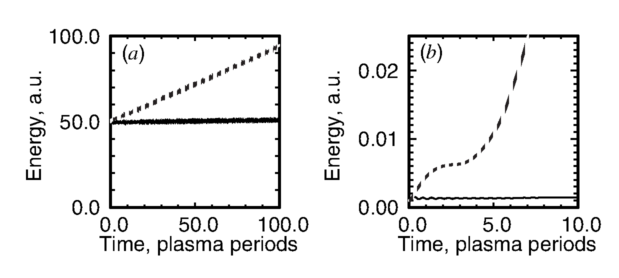
Figure 5: Energy conservation in VLPL code due to EC algorithm (solid lines) and numerical heating in standard MC algorithm (dashed lines) when (a) the Debye length $D=0.5\Delta x$, warm plasma and (b) $D=5\cdot 10^{-3}\Delta x$, cold plasma. Energy change in VLPL code is within 2% after 100 plasma periods.

The Fig. 5 shows the total energy evolution in an isolated system of particles for an energy conservative (solid lines) and a “momentum conservative” (MC) ([4]) (dashed lines) algorithms for the two cases: (a) Debye length is $D=0.5h$ and (b) $D=5\times 10^{-3}h$. Although the energy conservation for the EC algorithm is not exact, it is much better than for the MC case. The actual energy change is only 2% over 100 plasma oscillations for the EC algorithm. This property makes it possible to simulate a cold plasma.

7 Momentum and current conservation

It is known, that the energy-conserving electrostatic PIC codes do not conserve momentum [4]. Indeed, it is easy to show that, strictly speaking, the electric field interpolation to the particle position in the form of (42) does not conserve the total momentum

$$\frac{d{\bf P_{total}}}{dt}=\sum_{p}q_{p}E_{p}\neq 0,$$ (65)

if the particles cross cell boundaries during their motion.

Now the question is: how detrimental is this lack of momentum conservation for the PIC code?

The momentum nonconservation in electrostatic PIC codes using the $(\rho-\phi)$ formalism leads to impressive consequences [4]. If one starts the simulation with electrons drifting with respect to the resting ions, the electrons experience some average drag force from the grid. As a result, after a few plasma periods, an initially regular electron drift becomes chaotic and the simulation ends with disordered hot electrons without any net motion with respect to the ions. Although the final energy of the system is preserved, and remains the same as the initial kinetic energy of the drifting electrons, the momentum conservation failure is spectacular.

However, this spectacular example of momentum inconservation in the one-dimensional electrostatic PIC code is rather an artefact of the $(\rho-\phi)$ formalism. Moreover, even the inital “equilibrium” of electrons drifting with respect to ions is an artefact itself. Indeed, the original Maxwell equations (1)-(2) simply do not allow for freely drifting electrons in the one-dimensional geometry! This drift would correspond to a constant current, which results in a fast build-up of the longitudinal electric field. As a consequence, electrons must oscillate around their initial positions at the local plasma frequency. Apparently, this contradiction with the Maxwell equations remained unmentioned in the $(\rho-\phi)$ formulation of that electrostatic code.

In the more realistic $({\bf E-J})$ formalism of electromagnetic codes, the ions have to drift together with the electrons, unless the forward electron current is compensated by some artificial “return” current, e.g., the longitudinal part of ${\bf\nabla\times B}$, which evidently does not exist in the 1D geometry. Anyway, a code using the $({\bf E-J})$ conserves the net current per definition:

$$<{\bf J}>={\bf J_{0}}={\bf Const},$$ (66)

where the averaging is made in time over the local plasma frequency. Indeed, the only possible deviations in the current are due to the longitudinal part of electric field, i.e., the charge displacement current.

The current conservation (66) is the very important property, which may compensate for the absence of a detailed momentum conservation. As an example, let us consider the total electron current flowing in the simulation:

$${\bf J}_{e}=\sum_{p}eW_{p}{\bf V}_{p},$$ (67)

where $e$ is the electron charge, and $W_{p}$ is the “weight” of the numerical particle $p$. When averaged over plasma period, the current (67) is conserved by our code. Now, we may write the electron momentum in the non-relativistic case as

$${\bf P}_{e}=\sum_{p}m_{e}W_{p}{\bf V}_{p}=\frac{e}{m_{e}}{\bf J}_{e},$$ (68)

where $m_{e}$ is the electron mass.

It follows from (68) that the total momentum is simply proportional to the total current, and thus it is conserved on average. This is a good news for the energy conserving PIC code we have designed here. The code does conserve momentum on average in the non-relativistic case. When the particles are moving with relativistic energies, however, the identity (68) breaks, and the momentum conservation is not ideal again. Fortunately, the current conservation (67) is still a strong enough symmetry to prevent bad consequences like those discussed in [4].

8 Maxwell solver: Numerical Dispersion Free scheme

Earlier, we have discussed how to push particles and collect currents on the grid. Now, we are discussing the finite-difference solver for the time-dependent Maxwell Eqs. (2)-(1).

The standard approach to propagate the fields on Yee lattice, see Fig. 3 is to write the centered conservative scheme [4]. Let us first consider the two-dimensional geometry for the sake of simplicity. In the 2D $(X-Y)$ geometry, one may distinguish two kinds of polarizations, $s-$polarizations with $E_{z},B_{x},B_{y}$ fields, and $p-$polarization with $E_{x},E_{y},B_{z}$ fields. It can be shown, that if the initial condition contains $p-$polarized fields and $J_{x},J_{y}$ currents only, the $s-$polarized fields are not excited at all [4]. Thus, we may take the $p-$polarization as an example. The standard 2D scheme for the $p-$polarization is

$${B_{z}}_{i,j}^{n+1/2}-{B_{z}}_{i,j}^{n-1/2} = \frac{c\tau}{\Delta y}({E_{x}}_{i,j+1/2}^{n}-{E_{x}}_{i,j-1/2}^{n})$$ (69)

$$- \frac{c\tau}{\Delta x}({E_{y}}_{i+1/2,j}^{n}-{E_{y}}_{i-1/2,j}^{n}),$$

$${E_{x}}_{i,j+1/2}^{n+1}-{E_{x}}_{i,j+1/2}^{n} = \frac{c\tau}{\Delta y}({B_{z}}_{i,j+1}^{n+1/2}-{B_{z}}_{i,j}^{n+1/2})-4\pi\tau{j_{x}}_{i,j+1/2}^{n+1/2},$$ (70)

$${E_{y}}_{i+1/2,j}^{n+1}-{E_{y}}_{i+1/2,j}^{n} = \frac{c\tau}{\Delta x}({B_{z}}_{i+1,j}^{n+1/2}-{B_{z}}_{i,j}^{n+1/2})-4\pi\tau{j_{y}}_{i+1/2,j}^{n+1/2}.$$ (71)

The scheme (69)-(71) uses the centered expression for the finite difference ${\bf\nabla\times}$ operators like

$$\left({\bf\nabla\times B}_{z}\right)_{x}=\frac{1}{\Delta y}({B_{z}}_{i,j+1}^{n+1/2}-{B_{z}}_{i,j}^{n+1/2})$$ (72)

The Maxwell Eqs. 2)-(1) and the corresponding scheme (69)-(71) are essentially linear partial differential equation with the only nonlinear source terms in the form of the currents ${\bf j}$. In this case, we decide about quality of the finite difference scheme (69)-(71) comparing its dispersion properties with those of the Maxwell Eqs. themselves.

According to the Maxwell Eqs., all electromagnetic waves in vacuum run with the speed of light $c$. There is no dispersion in vacuum. Not so for the finite differences. We Fourier-analyze the scheme (69)-(71) by decomposing all the field in plane waves

$${\bf E} = \sum_{{\bf k}}{\bf E_{k}}\exp(-i\omega_{{\bf k}}t+i{\bf kx}),$$

$${\bf B} = \sum_{{\bf k}}{\bf B_{k}}\exp(-i\omega_{{\bf k}}t+i{\bf kx}),$$ (73)

where ${\bf k}$ is the wave vector, $\omega_{{\bf k}}$ the corresponding frequency, and ${\bf E_{k},B_{k}}$ amplitudes of the Fourier-harmonics. For the continuum Maxwell Eqs. we have the simple dispersion relation

$$\omega_{{\bf k}}=c|{\bf k}|,$$ (74)

while the discretization in the finite differences (69)-(71) introduces the numerical dispersion

$$\frac{1}{c^{2}\tau^{2}}\sin^{2}\frac{\omega_{{\bf k}}\tau}{2}=\frac{1}{\Delta x^{2}}\sin^{2}\frac{k_{x}\Delta x}{2}+\frac{1}{\Delta y^{2}}\sin^{2}\frac{k_{y}\Delta y}{2},$$ (75)

where $\Delta x$, $\Delta y$ are the grid steps, $\tau$ is the time step. The time step is limited by the Courant stability condition: $c^{2}\tau^{2}\leq\Delta x^{2}\Delta y^{2}/(\Delta x^{2}+\Delta y^{2})$. If we run the code close to this limit of stability, then only the waves propagating along the grid diagonals are dispersion-free. The largest numerical dispersion experience the waves running along the grid axises. This is illustrated in Fig. 6a, where we plot the phase velocity of the numerical modes, $V_{ph}=\omega_{k}/k$, for this standard scheme. We mention that we have chosen here $\Delta y=2\Delta x$, and this explains the evident asymmetry of the plot.

Although the numerical dispersion of the standard scheme might be not an issue when one simulates dense, nearly critical, plasma, it can make troubles for simulations of very underdense plasmas, as it is important for the problem of particle acceleration [17]. In the dense plasma case, the plasma dispersion is usually stronger than the numerical one, and the problem is masked. In the low-density plasma, however, the plasma dispersion is small. Yet, it has to be resolved accurately, as it influences the phase velocity of the laser pulse. As a consequence, one has to use many grid cells per laser wavelength to obtain physically correct results. Of course, one could send the laser along one of the grid diagonals, but this is extremely inconvenient from the programming point of view.

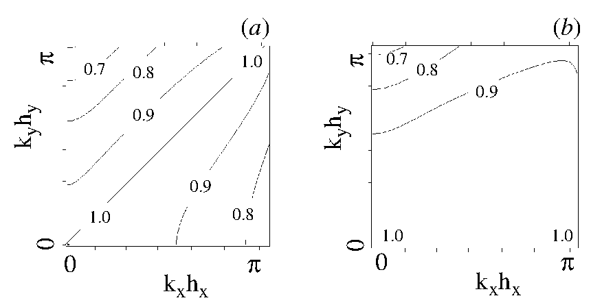
Figure 6: Numerical phase velocity $v_{ph}/c$ corresponding (a) to the standard scheme (75) and (b) to the NDFX scheme (81) used in the VLPL code. The grid cell aspect ratio $\Delta x/\Delta y=0.5$. The scheme (75) is dispersionless along the mesh diagonals, $k_{x}=k_{y}$, while the NDFX scheme (81) is dispersionless for waves running in $X-$direction when $k_{y}=0$.

We are now out for the design of a superior numerical scheme, which does not have a numerical dispersion at all, or removes it to a large extent. Let us return to the finite difference expression for the curl operator (72). This centered operator can be rewritten in a different way, using averages from the adjacent cells:

$$\left({\bf\nabla\times B}_{z}\right)_{x}\rightarrow\frac{1}{2\Delta y}({B_{z}}_{i+1,j+1}^{n+1/2}+{B_{z}}_{i-1,j+1}^{n+1/2}-{B_{z}}_{i+1,j}^{n+1/2}-{B_{z}}_{i-1,j}^{n+1/2}).$$ (76)

On the first sight, it is unclear, what did we gain from the averaging. It seems evident, that the averaged scheme (76) might have only worse dispersion than the simpler one (72). This is only partially correct.

It appears, however, that one may use a linear combination of the two schemes, (72) and (76), in such a way, that the dispersions of the two scheme compensate for each other! The resulting scheme for the $p-$polarization in the 2D geometry is

$${B_{z}}_{i,j}^{n+1/2} - {B_{z}}_{i,j}^{n-1/2}=\frac{c\tau}{\Delta y}(b_{x}({E_{x}}_{i,j+1/2}^{n}-{E_{x}}_{i,j-1/2}^{n})$$ (77)

$$+ a_{x}({E_{x}}_{i+1,j+1/2}^{n}-{E_{x}}_{i+1,j-1/2}^{n}+{E_{x}}_{i-1,j+1/2}^{n}-{E_{x}}_{i-1,j-1/2}^{n}))$$

$$- \frac{c\tau}{\Delta x}(b_{y}({E_{y}}_{i+1/2,j}^{n}-{E_{y}}_{i-1/2,j}^{n})$$

$$+ a_{y}({E_{y}}_{i+1/2,j+1}^{n}-{E_{y}}_{i-1/2,j+1}^{n}+{E_{y}}_{i-1/2,j-1}^{n}-{E_{y}}_{i-1/2,j-1}^{n})),$$

$${E_{x}}_{i,j+1/2}^{n+1} - {E_{x}}_{i,j+1/2}^{n}=\frac{c\tau}{\Delta y}({B_{z}}_{i,j+1}^{n+1/2}-{B_{z}}_{i,j}^{n+1/2})-4\pi\tau{j_{x}}_{i,j+1/2}^{n+1/2},$$ (78)

$${E_{y}}_{i+1/2,j}^{n+1} - {E_{y}}_{i+1/2,j}^{n}=\frac{c\tau}{\Delta x}({B_{z}}_{i+1,j}^{n+1/2}-{B_{z}}_{i,j}^{n+1/2})-4\pi\tau{j_{y}}_{i+1/2,j}^{n+1/2},$$ (79)

where the coefficients of the linear the combination of the two schemes is

$$a_{x} = a_{y}=0.125\frac{\Delta x}{\Delta y},$$

$$b_{x} = 1-2a_{x},$$

$$b_{y} = 1-2a_{y},$$ (80)

and we have supposed that $\Delta x\leq\Delta y$.

The dispersion relation for numerical scheme (77)-(79) is immediately found to be

$$\frac{1}{c^{2}\tau^{2}}\sin^{2}\frac{\omega\tau}{2} = \frac{1}{\Delta x^{2}}\sin^{2}\frac{k_{x}\Delta x}{2}(b_{y}+2a_{y}\cos k_{y}\Delta y)$$ (81)

$$+ \frac{1}{\Delta y^{2}}\sin^{2}\frac{k_{y}\Delta y}{2}(b_{x}+2a_{x}\cos k_{x}\Delta x).$$

It follows from (81) that the scheme is stable even at $c\tau=\Delta x$. This is a quite unique property for an explicit multi-dimensional finite-difference scheme. In addition, the scheme (81) goes over in the usual Yee scheme in the limit $\Delta_{x}/\Delta_{y}->0$.

When used close to the stability limit, the scheme completely removes numerical dispersion along the $X-$axis (the laser propagation direction). For this reason we call this scheme NDF: Numerical Dispersion Free [14]. The phase velocity of the numerical modes for the NDF scheme we plot in Fig. 6b. We mention, that the region where the numerical phase velocities are close to $c$ becomes much wider than for the standard scheme, Fig. 6a.

The plasma presence changes the stability condition slightly, and the maximum $\tau$ is limited to be:

$$1-\frac{\tau}{\Delta x}>\frac{\omega_{p}^{2}\tau^{2}}{4},$$ (82)

where $\omega_{p}=\sqrt{4\pi n_{e}e^{2}/m_{e}}$ is the maximum plasma frequency in the simulation domain. For an underdense plasma, however, this is an insignificant change.

The scheme (77)-(79) is written for the $p-$polarization in the 2D planar geometry. It is must be slightly modified before it can be used in the full 3D space. The final version of the 3D NDF scheme is:

$${B_{x}}_{i+1/2,j,k}^{n+1/2} - {B_{x}}_{i+1/2,j,k}^{n-1/2}=-\frac{c\tau}{\Delta y}(b_{z}({E_{z}}_{i+1/2,j+1/2,k}^{n}-{E_{z}}_{i+1/2,j-1/2,k}^{n})$$ (83)

$$+ a_{z}({E_{z}}_{i+1/2,j+1/2,k+1}^{n}-{E_{z}}_{i+1/2,j-1/2,k+1}^{n}+$$

$${E_{z}}_{i+1/2,j+1/2,k-1}^{n}-{E_{z}}_{i+1/2,j-1/2,k-1}^{n}))$$

$$+ \frac{c\tau}{\Delta z}(b_{y}({E_{y}}_{i+1/2,j,k+1/2}^{n}-{E_{y}}_{i+1/2,j,k-1/2}^{n})$$

$$+ a_{y}({E_{y}}_{i+1/2,j+1,k+1/2}^{n}-{E_{y}}_{i+1/2,j+1,k-1/2}^{n}+$$

$${E_{y}}_{i+1/2,j-1,k+1/2}^{n}-{E_{y}}_{i+1/2,j-1,k-1/2}^{n})),$$

$${B_{y}}_{i,j+1/2,k}^{n+1/2} - {B_{x}}_{i+1/2,j,k}^{n-1/2}=\frac{c\tau}{\Delta x}(b_{z}({E_{z}}_{i+1/2,j+1/2,k}^{n}-{E_{z}}_{i-1/2,j+1/2,k}^{n})$$ (84)

$$+ a_{z}({E_{z}}_{i+1/2,j+1/2,k+1}^{n}-{E_{z}}_{i-1/2,j+1/2,k+1}^{n}+$$

$${E_{z}}_{i+1/2,j+1/2,k-1}^{n}-{E_{z}}_{i-1/2,j+1/2,k-1}^{n}))$$

$$- \frac{c\tau}{\Delta z}(b_{x}({E_{x}}_{i,j+1/2,k+1/2}^{n}-{E_{x}}_{i,j+1/2,k-1/2}^{n})$$

$$+ a_{x}({E_{x}}_{i+1,j+1/2,k+1/2}^{n}-{E_{x}}_{i+1,j+1/2,k-1/2}^{n}+$$

$${E_{x}}_{i-1,j+1/2,k+1/2}^{n}-{E_{x}}_{i-1,j+1/2,k-1/2}^{n})),$$

$${B_{z}}_{i,j,k+1/2}^{n+1/2} - {B_{z}}_{i,j,k+1/2}^{n-1/2}=\frac{c\tau}{\Delta y}(b_{x}({E_{x}}_{i,j+1/2,k+1/2}^{n}-{E_{x}}_{i,j-1/2,k+1/2}^{n})$$ (85)

$$+ a_{x}({E_{x}}_{i+1,j+1/2,k+1/2}^{n}-{E_{x}}_{i+1,j-1/2,k+1/2}^{n}+$$

$${E_{x}}_{i-1,j+1/2,k+1/2}^{n}-{E_{x}}_{i-1,j-1/2,k+1/2}^{n}))$$

$$- \frac{c\tau}{\Delta x}(b_{y}({E_{y}}_{i+1/2,j,k+1/2}^{n}-{E_{y}}_{i-1/2,j,k+1/2}^{n})$$

$$+ a_{y}({E_{y}}_{i+1/2,j+1,k+1/2}^{n}-{E_{y}}_{i-1/2,j+1,k+1/2}^{n}+$$

$${E_{y}}_{i-1/2,j-1,k+1/2}^{n}-{E_{y}}_{i-1/2,j-1,k+1/2}^{n})),$$

$${E_{x}}_{i,j+1/2,k+1/2}^{n+1} - {E_{x}}_{i,j+1/2,k+1/2}^{n}=\frac{c\tau}{\Delta y}(b_{z}({B_{z}}_{i,j+1,k+1/2}^{n+1/2}-{B_{z}}_{i,j,k+1/2}^{n+1/2})$$ (86)

$$+ a_{z}({B_{z}}_{i,j+1,k+3/2}^{n+1/2}-{B_{z}}_{i,j,k+3/2}^{n+1/2}+{B_{z}}_{i,j+1,k-1/2}^{n+1/2}-{B_{z}}_{i,j,k-1/2}^{n+1/2}))$$

$$- \frac{c\tau}{\Delta z}(b_{y}({B_{y}}_{i,j+1/2,k+1}^{n+1/2}-{B_{y}}_{i,j+1/2,k}^{n+1/2})$$

$$+ a_{y}({B_{y}}_{i,j+3/2,k+1}^{n+1/2}-{B_{y}}_{i,j+3/2,k}^{n+1/2}+{B_{y}}_{i,j-1/2,k+1}^{n+1/2}-{B_{y}}_{i,j-1/2,k}^{n+1/2}))$$

$$- 4\pi\tau{j_{x}}_{i,j+1/2,k+1/2}^{n+1/2},$$

$${E_{y}}_{i+1/2,j,k+1/2}^{n+1} - {E_{y}}_{i+1/2,j,k+1/2}^{n}=-\frac{c\tau}{\Delta x}(b_{z}({B_{z}}_{i+1,j,k+1/2}^{n+1/2}-{B_{z}}_{i,j,k+1/2}^{n+1/2})$$ (87)

$$+ a_{z}({B_{z}}_{i+1,j,k+3/2}^{n+1/2}-{B_{z}}_{i,j,k+3/2}^{n+1/2}+{B_{z}}_{i+1,j,k-1/2}^{n+1/2}-{B_{z}}_{i,j,k-1/2}^{n+1/2}))$$

$$+ \frac{c\tau}{\Delta z}(b_{x}({B_{x}}_{i+1/2,j,k+1}^{n+1/2}-{B_{x}}_{i+1/2,j,k}^{n+1/2})$$

$$+ a_{x}({B_{x}}_{i+3/2,j,k+1}^{n+1/2}-{B_{x}}_{i+3/2,j,k}^{n+1/2}+{B_{x}}_{i-1/2,j,k+1}^{n+1/2}-{B_{x}}_{i-1/2,j,k}^{n+1/2}))$$

$$- 4\pi\tau{j_{y}}_{i+1/2,j,k+1/2}^{n+1/2},$$

$${E_{z}}_{i+1/2,j+1/2,k}^{n+1} - {E_{z}}_{i+1/2,j+1/2,k}^{n}=\frac{c\tau}{\Delta x}(b_{y}({B_{y}}_{i+1,j+1/2,k}^{n+1/2}-{B_{y}}_{i,j+1/2,k}^{n+1/2})$$ (88)

$$+ a_{y}({B_{y}}_{i+1,j+3/2,k}^{n+1/2}-{B_{y}}_{i,j+3/2,k}^{n+1/2}+{B_{y}}_{i+1,j-1/2,k}^{n+1/2}-{B_{y}}_{i,j-1/2,k}^{n+1/2}))$$

$$- \frac{c\tau}{\Delta y}(b_{x}({B_{x}}_{i+1/2,j+1,k}^{n+1/2}-{B_{x}}_{i+1/2,j,k}^{n+1/2})$$

$$+ a_{x}({B_{x}}_{i+3/2,j+1,k}^{n+1/2}-{B_{x}}_{i+3/2,j,k}^{n+1/2}+{B_{x}}_{i-1/2,j+1,k}^{n+1/2}-{B_{x}}_{i-1/2,j,k}^{n+1/2}))$$

$$- 4\pi\tau{j_{z}}_{i+1/2,j+1/2,k}^{n+1/2},$$

where we are using the following expressions for the free parameters $a_{\alpha},b_{\alpha}$:

$$a_{x} = a_{y}+a_{z},$$

$$a_{y} = 0.125\frac{\Delta x}{\Delta y},$$

$$a_{z} = 0.125\frac{\Delta x}{\Delta z},$$

$$b_{x} = 1-2a_{x},$$

$$b_{x} = 1-2a_{y},$$

$$b_{x} = 1-2a_{z}.$$ (90)

Here we have chosen the coefficients (90) in such a way, that the scheme is stable provided $\Delta x\leq\Delta y,\Delta z$, and the numerical dispersion is removed for waves running along $X-$axis.

9 Lorentz boost

The plasma-based particle acceleration is a multi-scale problem, and the scales are very disparate, see Fig. 7. The smallest scale is the laser wavelength $\lambda$ in the case of the laser-drieven acceleration, or the plasma wavelength $\lambda_{p}$ for beam-driven plasma wake fields. The laser wavelength is on the order of micrometers, while the plasma wavelength can be from tens of micrometers to millimeters. The medium scale is the driver length. It can be comparable to the plasma wavelength in the case of the bubble [16] and blowout [15] regime, or be much longer when we rely on self-modulation in plasma [19, 20, 21, 22]. The largest scale is the acceleration length that can range from centimeters to hundereds of meters or even kilometers [17]. It is this discrepancy between the driver scale and the acceleration distance that makes the simulations rather expensive.

One of the possibilities to bring the scales together is to change the reference frame form the laboratory one to the co-moving with the driver. This is called the Lorentz boost technique [23]. Let us assume, we transform from the laboratory frame $L$ into a frame $R$ moving in the propagation direction of the driver. The relative velocity of the $R-$frame is $V=\beta c$ and its relativistic factor is $\gamma=1/\sqrt{1-\beta^{2}}$. Then, the driver is Lorentz-stretched in the $R-$frame with the factor $\gamma(1+\beta)$ and the propagation length is compressed with the same factor, see Fig. 7. Thus, potentially, the Lorentz-transformation allows us to increase the longitudinal grid step and time step - provided it is the grid step that limits the time step - and we have smaller distance to propagate. The overall increase in performace could be huge.

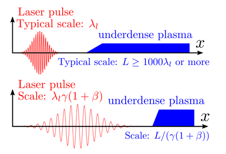
Figure 7: Scales discrepancy in plasma-based acceleration. Transformation into a co-moving frame reduces the scales discrepancy.

Unfortunately, the background plasma becomes streaming in the $R-$frame with the same transformation velocity $-V$. The plasma density is higher in the $R-$frame than in the laboratory frame by the factor $\gamma$. This leads to a source of free energy that can be converted into numerical plasma heating as the plasma particles interact with the numerical spatial grid. The associated numerical instability can have a rather effect on the simulation quality [24]. The numerical noise generated by the unstable modes can completely mask the regular wake structure as shown in the example in Fig. 8.

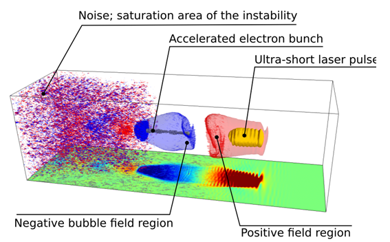
Figure 8: 3D view of a numerical instability caused by plasma streaming in the co-moving frame.

The main reason for the numerical instability is the Cerenkov resonance between the streaming plasma particles and the numerical electromagnetic modes on the grid. The numerical electromagnetic modes have subluminal phase velocities and can be in particle-wave resonance with the macroparticles of the background plasma that stream through the grid with the relativistic factor $\gamma$. The mechanism of the numerical instability is illustrated in Fig. 9a). Plasma fluctuations deviate particles from the straight line trajectory. This leads to transverse currents. The transverse currents cause electromagnetic fields. Some of these electromagnetic modes propagate exactly at the particle velocity and can resonantly exchange energy with the particles. This is the Cerenkov mechanism.

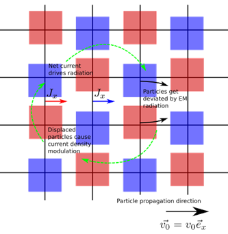
Figure 9: 3D view of a numerical instability caused by plasma streaming in the co-moving frame.

One can solve the wave-particle dispersion relation for the standard Yee electromagnetic solver and calculate growth rate of the instability analytically. A comparison of the observed electromagnetic modes in a PIC simulation and of the analytical prediction is shown in Fig. 10. Thus, indeed, the reason for the numerical instability is the Cerenkov resonance between the relativistically moving plasma particles and numerical electromagnetic modes that have subluminal phase velocities on the Yee grid.

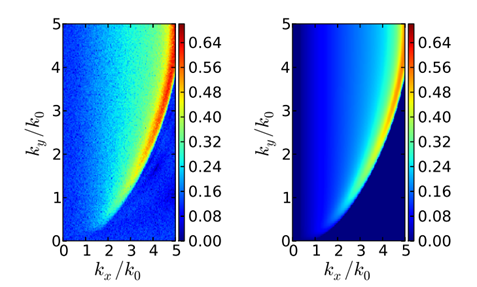
Figure 10: Left pane: observed growing modes in a PIC simulation, Right pane: analytically calculated growth rate of Cerenkov-unstable modes.

One might hope to remove the instability by choosing a different Maxwell solver. One could take for example a dispersion-free solver based on Fourier transformation. Indeed, a dispersion-free solver reduces the instability growth rate. Unfortunately, it does not eliminate it completely. The reason is the spatial and temporal aliasing on the grid. The relativistic particle starts to interact with the numerical modes from the other Brillouin zones.

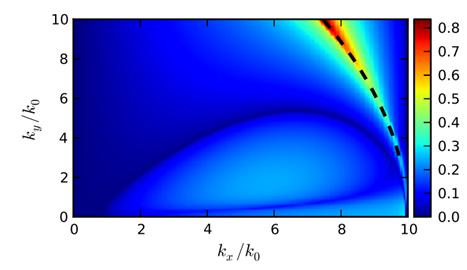
Figure 11: Observed growing modes in a PIC simulation (the color scale) and the analytic resonance condition due to the grid aliasing (the broken line).

One can write the non-resolved aliased frequencies of the numerical grid as

$$\omega_{eff}=\pm\left(\sqrt{k_{x}^{2}+k_{y}^{2}}-\frac{1}{\Delta t}\right)$$ (91)

where $\Delta t$ is the time step. The resonance condition is then fulfilled for electromagnetic waves with the wave numbers

$$k_{y}\left(k_{x}\right)=\frac{1}{h}\sqrt{h^{2}k_{x}^{2}\left(v_{0}^{2}-1\right)-2hk_{x}v_{0}^{2}+v_{0}^{2}}$$ (92)

where $h$ is the grid step. The analytic resonance curve and the growing modes observed in a numerical experiment are shown in Fig. 11.

The only viable way of taming the numerical instability in Lorentz-boosted simulations is applying low-pass filters to the deposited currents before the electromagnetic fields are updated at every time step. The filtering reduces the instability to acceptable levels. Yet, a heavy filtering of the currents can in turn influence dispersion of numerical modes so that one has to be very careful [25].

10 Quasi-static codes

Another possibility to bridge the gap between disparate scales in plasma-based acceleration is using the quasi-static approximation. It separates explicitly the fast scale of the driver and the slow scale of acceleration [26]. To do so, we introduce the new variables

$$\tau = t$$ (93)

$$\zeta = z-ct$$ (94)

We assume that the driver changes slowly as it passes its own length. Thus, as we calculate plasma response to the driver, we neglect all derivatives over the slow time $\tau$ and we advance from the front of the driver to the tail to calculate the wake field configuration at a particular time $\tau$. As we find the fields and the plasma particles distribution, we can advance the driver with a large time step in $\tau$. This procedure increases the code performance by many orders of magnitude. Simulations of large scale plasma-based acceleration that required huge massively parallel computers with the explicit PIC, can be done on a desktop workstation in the quasi-static approximation. Of course, the quasi-static approximation is limited as it does not describe radiation, but the static electromagnetic fields only.

The first quasi-static particle-in-cell code WAKE has been written by Mora and Antonsen [26]. It was a 2D code in cylindrical geometry and use equations written in terms of the wake potential and the magnetic field. Later, a full 3D code Quick-PIC has been developed that used the same equations[27]. Another 2D code in cylindrical gemetry LCODE has been developed by Lotov and used equations on fields directly [28]. Here we show formalism used by the quasi-static version of the code VLPL. It is a full 3D code in Cartesian geometry. Like the LCODE, it uses equations on the fields. Below we derive the quasi-static field equations.

We start again with the Maxwell equations Ampere-Bcharge and write them in the new variables eq:tau-eq:zeta neglecting derivatives with respect to the slow time $\tau$:

$$c\nabla\times{\bf B} = -c\frac{\partial{\bf E}}{\partial\zeta}+4\pi{\bf j},$$ (95)

$$c\frac{\partial{\bf B}}{\partial\zeta} = c\nabla\times{\bf E},$$ (96)

$$\nabla\cdot{\bf E} = 4\pi\rho,$$ (97)

$$\nabla\cdot{\bf B} = 0.$$ (98)

First, we take curl of the Ampere law Ampere-1 and $\zeta$-derivative of the Faraday law Faraday-1. Combining these two equations, we arrive at the first quasi-static equation on the magnetic field:

$$\nabla_{\perp}^{2}{\bf B} = -\frac{4\pi}{c}\nabla\times{\bf j},$$ (99)

where the $\nabla_{\perp}$ operator acts on coordinates transversal to the propagation direction.

Now, we take gradient of the Poisson law Poisson-1. We use the well-known identity from vector analysis $\nabla\left(\nabla\cdot{\bf E}\right)=\nabla^{2}{\bf E}+\nabla\times\nabla\times{\bf E}$ and obtain for the transverse components of the electric field the equation

$$\nabla_{\perp}^{2}{\bf E}_{\perp} =4\pi\left(\nabla_{\perp}\rho-\frac{1}{c}\partial_{\zeta}{\bf j_{\perp}}\right)$$ , (100)

For the longitudinal electric field component we obtain

$$\nabla_{\perp}^{2}E_{||} =4\pi\frac{\partial}{\partial{\zeta}}\left(\rho-\frac{1}{c}j_{||}\right) =\frac{4\pi}{c}\nabla_{\perp}\cdot{\bf j_{\perp}},$$ (101)

where also used the continuity equation

$$\frac{\partial}{\partial{\zeta}}\rho =\frac{\partial}{\partial{\zeta}}j_{||}+\nabla_{\perp}\cdot{\bf j_{\perp}}$$ (102)

The continuity equation eq:QS cont can be used to remove the charge density $\rho$ from the quasi-static equations and work with the currents only. This may reduce the noise in particle-in-cell codes.

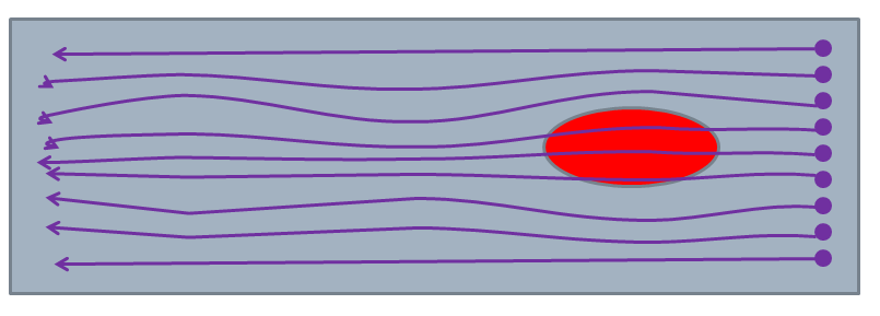
Figure 12: Left pane: observed growing modes in a PIC simulation, Right pane: analytically calculated growth rate of Cerenkov-unstable modes.

A typical quasi-static PIC code works a s following. First, the charge density and currents generated by the driver on the numerical grid are gathered. These are the sources that contribute to the basic equations eq:QS B-eq:QS Epar. Then, a layer of numerical macroparticles is seeded at the front boundary (the head of the driver) of the simulation box. These numerical particles advance in the negative $\zeta-$direction (towards the tail of the driver) according to the Eqs. eq:QS B-eq:QS Epar. As the plasma particles pass the whole simulation domain, the fields and density are defined on the grid and can be used to advance in time $\tau$ the driver.

If the driver is a charged particle beam, then we solve equations of motion for beam particles in the calculated plasma fields. If the driver is a laser pulse, one has to solve an envelope equation on the laser pulse amplitude. This is required, because the quasi-static equations do not describe radiation. Thus, an independent analytical model is required for the laser pulse. The laser pulse vector potential is represented as ${\bf A}({\bf\tau,\zeta,r})=\Re\left[{\bf a}({\bf\tau,\zeta,r})\exp\left({\bf i}k\zeta\right)\right]$. The envelope equation on the complex amplitude ${\bf a}({\bf\tau,\zeta,r})$ reads as [26]:

$$\left[\frac{2}{c}\frac{\partial}{\partial\tau}\left({\bf i}k_{0}+\frac{\partial}{\partial\zeta}\right)+\nabla_{\perp}^{2}\right]{\bf a}=\chi({\bf\zeta,r})$$ (103)

where $\chi({\bf\zeta,r})=<4\pi q^{2}n/\gamma mc^{2}>$ is the plasma refraction averaged over all the particles in the cell with the charges $q$, masses $m$, and relativistic factors $\gamma$.

The laser pulse acts on the plasma particles via its ponderomotive force

$$F_{p}=-\frac{q^{2}}{\gamma mc^{2}}\nabla a^{2}$$ (104)

The ponderomotive force eq:ponderomotive is added to the standard Lorentz force in the particle pusher.

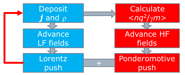
Figure 13: The typical time step of a quasi-static code. The cycle for low frequency (LF) plasma fields is followed by the cycle for envelope equation on the high frequency (HF) laser driver.

The typical time step of a quasi-static code is shown in Fig. 13. First, there is a cycle along the fast variable $\zeta$ for the low frequency (LF) fields. Then, the plasma refraction is calculated and the envelope equation for the high frequency (HF) fields is updated.

Fig. 14 shows a comparison between the quasi-static code (the upper half of the simulation) and the full PIC code VLPL3D. We have simulated a blow-out generated by an overdense electron bunch. The electron bunch density had the profile $n_{b}(z,{\bf r})=n_{b0}\exp\left(-z^{2}/2\sigma_{z}^{2}\right)\exp\left(-r^{2}/2\sigma_{r}^{2}\right)$. The maximum bunch density was two times higher than the background plasma density: $n_{b0}=2n_{p}$. The bunch was spherical with $k_{p}\sigma_{z}=k_{p}\sigma_{r}=1$.

Figure 14: Blow-out wake field generated by an overdense electron bunch. The upper half of the frame is taken a quasi-static code simulation. The lower part is taken from a full PIC code VLPL3D simulation. The left frame shows the plasma density, the right frame shows the longitudinal electric field component of the wake field. Cerenkov radiation emitted by the wave breaking point. is seen in the full 3D PIC simulation. This radiation is absent in the quasi-static code.

The both simulations are nearly identical. The only significant difference is the presence of Cerenkov radiation in the full 3d PIC simulation from the wave breaking point at the very tail of the first bubble. In the full simulation, we initialized the electron bunch vacuum in front of the plasma layer. Thus, the plasma layer had to have a density ramp. The length of the bubble depends on the plasma density: the higher the density, the shorter the bubble. Consequently, the wavebreaking point moved with a superluminal velocity in the density ramp region and could emit the Cerenkov radiation. In the quasi-static code, the Cerenkov radiation cannot be simulated. In addition, no density ramp is needed there: the field distribution is defined by the local plasma density and by the instantaneous shape of the driver only.

11 Computational costs of different codes

It is useful to estimate the number of operations required to simulate a particular plasma based acceleration problem with different codes. We call it the computational cost. The most general one, the full 3D PIC code, uses a 3D spatial grid of the size $N_{||}\times N_{\perp}^{2}$ cells and $N_{t}$ time steps. The longitudinal step is limited by the laser wavelength, $h_{||}\ll\lambda_{0}$ and the corresponding time step $\tau\ll\lambda_{0}/c$. The transverse grid steps are usually limited by the plasma wavelength, $h_{\perp}\ll\lambda_{p}$ . The number of time steps is $N_{t}=L_{acc}/c\tau$, where $L_{acc}$ is the acceleration distance. Thus, the number of operations required by the explicit PIC code scales as

$$N_{op}^{PIC}\propto\frac{L_{acc}l_{d}}{\lambda_{0}^{2}}N_{\perp}^{2}$$ (105)

Here, we assumed that the “moving window” technique is used so that the longitudinal size of the simulation box $l_{d}$ scales with the plasma wavelength $\lambda_{p}$.

If one uses the Lorentz boost technique with the transformation relativistic factor $\gamma_{boost}$, the number of required operations reduces by the factor $\gamma_{boost}^{2}$ ideally:

$$N_{op}^{PIC\,LB}\propto\gamma_{boost}^{-2}\frac{L_{acc}l_{d}}{\lambda_{0}^{2}}N_{\perp}^{2}=\gamma_{boost}^{-2}N_{op}^{PIC}$$ (106)

The quasi-static approximation alleviates the time step restriction by the Courant condition. In addition, the grid step is no more limited by the laser wavelength $\lambda_{0}$, but rather by the plasma wavelength $\lambda_{p}$. The time step must resolve the betatron oscillation of the beam particles, $\tau\omega_{\beta}\ll 1$, where the betatron frequency for a beam particle with the mass $M$ and relativistic factor $\gamma_{b}$ is $\omega_{\beta}=\omega_{p}\sqrt{m_{e}/2\gamma_{b}M}$. If the driver is a laser pulse, then the time step must resolve the diffraction length, $c\tau/Z_{R}\ll 1$, where the characteristic diffraction length of a laser pulse with the focal spot $R$ is defined by the Rayleigh length $Z_{R}=\pi R^{2}/\lambda_{0}$. The overall number of operations required by the quasi-static code scales as

$$N_{op}^{QS}\propto\frac{L_{acc}\omega_{\beta}}{c}\frac{l_{d}}{\lambda_{p}}N_{\perp}^{2}=\frac{\lambda_{0}^{2}}{\lambda_{p}\lambda_{\beta}}N_{op}^{PIC}$$ (107)

where $\lambda_{\beta}=2\pi c/\omega_{\beta}$ is the betatron wavelength. The performance gain $\lambda_{0}^{2}/\lambda_{p}\lambda_{\beta}$ of the quasi-static codes over the fully explicit PIC can be huge and easily reach six orders of magnitude.

12 The future of PIC codes

Electromagnetic particle-in-cell codes provide a very fundamental model the dynamics of ideal plasma. Particularly in the relativistic regime of short pulse laser-plasma interactions, these codes are unique in the predictive capabilities. In this regime, the binary collisions of plasma particles are either negligible or can be considered as a small perturbation and thus the electromagnetic PIC codes are the most adequate tools.

Yet, the explicit PIC codes have their limits. As soon as one tries to simulate laser interactions with highly overdense plasmas, these PIC codes becomes extremely expensive. Indeed, because the scheme is explicit, the code must resolve the plasma frequency and the skin depth. Even for uncompressed solid targets of high-Z materials, the plasma frequency may easily be 30 times higher than the laser frequency. Correspondingly must be chosen the time and grid steps. For a 3D code, the simultaneous refinement of the grid and time steps in all dimensions by a factor $\alpha$ leads to the computational effort increase by the factor $\alpha^{4}$. For this reason, the simulation of a highly overdense plasma is still a challenge for the explicit PIC codes.

A way around this difficulty might give implicit PIC codes, like the code LSP [29], or hybrid, i.e., a mixture of a hydrodynamic description of the high-density background plasma and PIC module for the hot electrons and ions [30]. These codes alleviate the time step limitation, because they suppose the background plasma to be quasi-neutral and thus eliminate the fastest plasma oscillations at the Langmuir frequency. Very large plasma regions of high density can be easily simulated using these codes. Yet, these codes sacrifice a lot of physics and for each particular problem it must be checked whether this omitted physics is important or not. One of the possibilities to do this check is to benchmark the results of implicit codes against the direct PIC on model problems, which can be simulated by the both types of the codes.

13 Aknowledgements

This work has been supported by EU FP7 project EUCARD-2 and by BMBF, Germany.

References

- [1] A Pukhov, Reports on progress in Physics 66, 47 (2001).
- [2] J. Villasenor and O. Buneman, Comp. Phys. Comm., 69, 306 (1992).
- [3] J. Dawson, Reviews Modern Phys. 55, 403 (1983).
- [4] C. K. Birdsall and A. B. Langdon, Plasma physics via computer simulations (Adam Hilger, New York, 1991).
- [5] R. W. Hockney & J. W. Eastwood, Computer Simulation Using Particles 540 S. (London: McGraw Hill 1981).
- [6] J. D. Jackson, Classical electrodynamics, N.Y.: Whiley p.848, (1975).
- [7] L.Landau and E.~Lifshitz, The Classical Theory of Fields, 2nd ed. Addison-Wesley, Reading, Mass., (1962).
- [8] N. A. Krall and A. W. Trivelpiece, Principles of plasma physics, McGraw-Hill, N.Y. (1973).
- [9] S. I. Braginskii, Transport properties in a plasma, in M. A. Leontovich (ed.) “Review of plasma physics”, Consult. Bureau, N.Y. (1965).
- [10] A. A. Vlasov, Many-Particle Theory and Its Application to Plasma, Gordon and Breach, 1961.
- [11] H. Ruhl, P. Mulser, Phys. Lett. A205, 388 (1995); P. Bertrand, A. Ghizzo, T. W. Johnston, M. Shoucri, E. Fijalkov, and M. R. Feix, Phys. Fl. B, 5, p.1028 (1990).
- [12] R.C. Morse, C.W. Nielsen, Phys. Fluids, 14, p. 830 (1971)
- [13] R. H. Cohen, A. Friedman, D. P. Grote and J. L. Vay, Nucl. Instrum. Methods Phys. Res. A 606 53–5 (2008)
- [14] A. Pukhov, Journal of Plasma Physics, accepted for publication (1999).
- [15] K. V. Lotov, Phys. Rev. E 69, 046405 (2004)
- [16] A. Pukhov and J. Meyer-ter-Vehn Applied Physics B 74, p. 355-361 (2001)
- [17] E. Esarey, C. B. Schroeder, and W. P. Leemans, Rev. Mod. Phys. 81, 1229 (2009)
- [18] F. F. Chen, Introduction to plasma physics and controlled fusion, N.Y.:Plenum Press (1984).
- [19] Joshi, C., T. Tajima, J. M. Dawson, H. A. Baldis, and N. A. Ebrahim, Phys. Rev. Lett. 47, 1285 (1981).
- [20] Andreev, N. E., L. M. Gorbunov, V. I. Kirsanov, A. A. Pogosova, and R. R. Ramazashvili, Pis’ma Zh. Eksp. Teor. Fiz. 55, 551 (1992).
- [21] Antonsen, T. M., Jr., and P. Mora, Phys. Rev. Lett. 69, 2204 (1992).
- [22] A Pukhov, N Kumar, T Tückmantel, A Upadhyay, K Lotov, P Muggli Physical review letters 107, 145003 (2011)
- [23] Vay J-L Phys. Rev. Lett. 98 130405 (2007)
- [24] Vay J L, Geddes C G R, Cormier-Michel E and Grote D P J. Comput. Phys. 230 5908–29 (2011)
- [25] B. B. Godfrey and J. L. Vay, arXiv:1502.01387v1 (2015)
- [26] P. Mora, T. M. Antonsen, Phys. Plasmas 4, 217 (1997)
- [27] C. Huang, V.K. Decyk, C. Ren, M. Zhou, W. Lu, W.B. Mori, J.H. Cooley, T.M. Antonsen Jr., T. Katsouleas, Journal of Computational Physics 217, 658–679 (2006)
- [28] K.V. Lotov, Phys. Rev. ST Accel. Beams 6 061301 (2003).
- [29] D. R. Welch, D. V. Rose. B. V. Oliver, and R. E. Clark, Nucl. Instr. Meth. Phys. Res. A 464, 134 (2001).
- [30] T Tückmantel, A Pukhov, Journal of Computational Physics 269, 168-180 (2014)