Deep GALEX UV Survey of the Kepler Field I: Point Source Catalog

Abstract

We report observations of a deep near-ultraviolet (NUV) survey of the Kepler field made in 2012 with the Galaxy Evolution Explorer (GALEX) Complete All-Sky UV Survey Extension (CAUSE). The GALEX-CAUSE Kepler survey (GCK) covers 104 square degrees of the Kepler field and reaches limiting magnitude NUV $\simeq$ 22.6 at 3$\sigma$. Analysis of the GCK survey has yielded a catalog of 669,928 NUV sources, of which 475,164 are cross-matched with stars in the Kepler Input Catalog (KIC). Approximately 327 of 451 confirmed exoplanet host stars and 2614 of 4696 candidate exoplanet host stars identified by Kepler have NUV photometry in the GCK survey. The GCK catalog should enable the identification and characterization of UV-excess stars in the Kepler field (young solar-type and low-mass stars, chromospherically active binaries, white dwarfs, horizontal branch stars, etc.), and elucidation of various astrophysics problems related to the stars and planetary systems in the Kepler field.

I. Introduction

The fast growth of exoplanet detections has motivated the derivation of more accurate fundamental stellar properties (e.g. mass, radius, age, etc.) and the connection between these properties and those of their evolving planetary systems. The precision with which the exoplanets’ parameters can be estimated directly depends on the precision associated to the properties of their stellar hosts. Of particular importance is the stellar age, since one of the major goals in the study of exoplanetary systems is to establish their evolutionary stage, and how this compares to the properties of our own solar system.

Reliably age-dating solar-type field stars is notoriously difficult. For these stars, alternative methods to isochrone fitting techniques have been explored. Chromospheric activity and stellar rotation are among the more reliable observables for stellar age estimation of Sun-like main sequence stars. The most common and accessible proxy for stellar activity has been the emission in the Ca II resonance line in the optical-ultraviolet spectral interval (e.g. Mamajek & Hillenbrand, 2008). Alternative proxies have also been identified and include the high contrast emission of Mg II line in the ultraviolet (UV) and the continuum UV excess (e.g. Findeisen et al., 2011; Olmedo et al., 2013). For these stars, ultraviolet radiation originates in the hot plasma of the upper stellar atmospheres at temperatures of $\sim 10^{4}-10^{6}$ K, heated by non-thermal mechanisms, such as acoustic and magnetic waves, generated by convection and rotation (e.g. Narain & Ulmschneider, 1996; Ulmschneider & Musielak, 2003). As the star ages, it loses angular momentum due to magnetic braking (Mestel, 1968; Kawaler, 1988), slowing the rotation and affecting the stellar dynamo, which in turn decreases the magnetic field leading to a decrement of the UV emission. In this first paper of a series aimed at investigating the UV properties of stars, we present a complete catalog of UV sources detected by the Galaxy Evolution Explorer (GALEX; Martin et al., 2005; Bianchi et al., 2014) in the field of the Kepler Mission (Basri et al., 2005).

The Kepler field (i.e., the 100 square degree field of the original Kepler mission) has been fully surveyed at different optical and infrared bandpasses (Lawrence et al., 2007; Brown et al., 2011; Everett et al., 2012; Greiss et al., 2012). Its stellar content, mainly comprised of field stars, with over 450 confirmed exoplanet host stars, has rapidly become one of the most studied stellar samples and regions of the sky. The Kepler  field and associated survey data comprise a potentially valuable resource for studying the age-activity-rotation relation for low-mass stars. Rotation periods (and ages) of stars in the Kepler field have been determined in a number of studies (e.g. Reinhold et al., 2013; Walkowicz & Basri, 2013; García et al., 2014; McQuillan et al., 2014; do Nascimento et al., 2014; Meibom et al., 2015).

The GALEX UV space observatory was launched in 2003 and was operated by NASA until 2011 (Martin et al., 2005; Bianchi et al., 2014). Afterwards, the GALEX mission was managed by Caltech for about a year as a private space observatory, until the satellite was turned off in June 2013. GALEX is a 50 cm Ritchey-Chrétien telescope with a 1^∘.25 wide field-of-view, equiped with a near-UV (NUV; 1771-2831 Å, $\lambda_{\rm eff}$ = 2271 Å) and a far-UV (FUV; 1344-1786 Å, $\lambda_{\rm eff}$ = 1528 Å) detectors. During it’s main mission, GALEX carried out the All-Sky, Medium, and Deep Imaging Surveys, with exposure times of $\sim$100, $\sim$1000, and $>$10000 sec, respectively, measuring more than 200 million sources (Bianchi et al., 2014). The continuation phase, called the GALEX Complete All-Sky UV Survey Extension (CAUSE), was funded by several consortia, with the main goal of extending observations in the NUV band to the Galactic plane, which was only scarcely mapped during the main mission, due to restrictions on the maximum target brightness.

In this work, we describe the creation of a deep NUV photometric catalog with nearly full coverage of the Kepler field using CAUSE observations. In Section II we introduce the observations, and characteristics of the data. In Section III we explain the procedure for extracting the NUV point sources. Section IV describes the point source catalog, and its crossmatch with the Kepler Input Catalog (KIC) and the Kepler Objects of Interest (KOI) catalog is presented in Section V. Finally, the publicly available GALEX-CAUSE (GCK) catalog of NUV sources is described in Section VI.

II. Observations

As part of the CAUSE survey, Cornell University funded 300 orbits to complete the spatial coverage of the Kepler field through August-September 2012 (PI J. Lloyd). The dataset of GALEX CAUSE Kepler field observations (hereafter GCK) is composed of 180 tiles that cover the Kepler field (Borucki et al., 2003; Basri et al., 2005; Brown et al., 2005; Latham et al., 2005); each tile has 20 visits on average. These observations sample timescales from a millisecond to a month, and can be used to identify variable targets and exotic sources on such timescales. The GCK dataset provides spatial coverage of the Kepler field in the GALEX NUV band.

The standard GALEX pointed observation mode adopted for the surveys during the primary NASA GALEX  mission employed a 1′.5 spiral dither pattern. This dither moves the sources with respect to detector artifacts and prevents a bright source to saturate one position on the detector, which is subject to failure if overloaded. The GALEX data pipeline processes the photon arrival times and positions with an attitude solution that reconstructs an image of the sky for a single tile, 1^∘.2 in diameter around the pointing center.

In 2012, a drift mode was adopted, which scanned a strip of the sky along a great circle. For GCK observations, these scans run as long as 12^∘. The scan mode processing uses a pipeline adapted from the pointed mode observations. To adapt the scans to the standard tile processing pipeline, they are processed in tile sized images resulting in 9 and 14 images for the short scans (1$-$3 and 13$-$15) and long scans (4$-$12), respectively (shown in Fig. 1). Thus for the 180 tiles of the GCK data, with each visited an average of 20 times, we have a total of $\sim$ 3200 images.

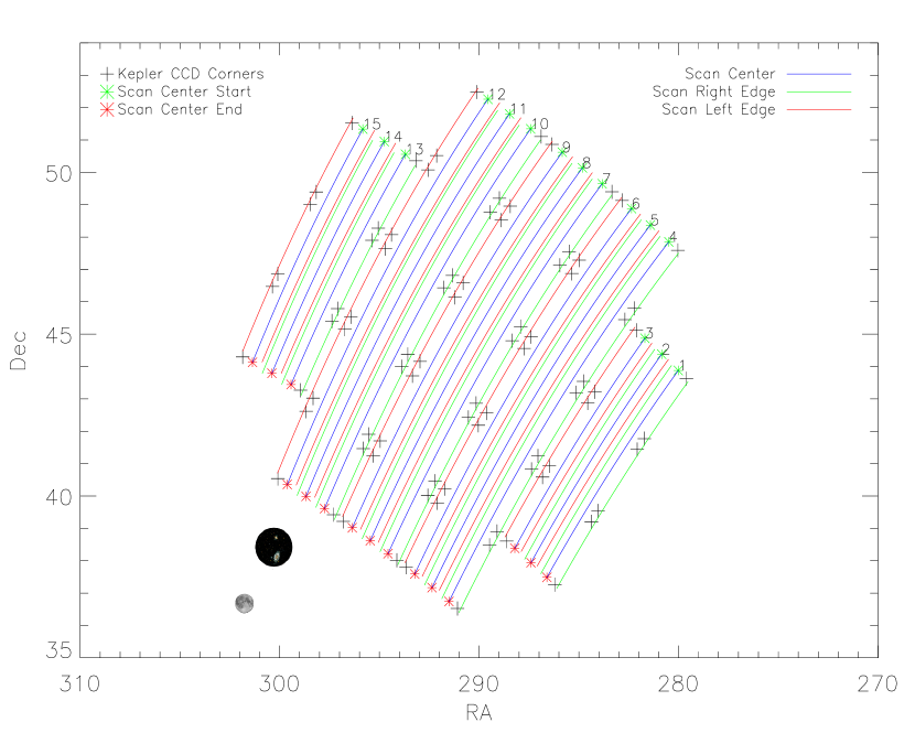
Figure 1.— Scan mode observations of GCK survey covering the Kepler field. The field of view of GALEX and a full moon are shown for comparison. The numbers on the upper right edges correspond to the scan numbers. The plus symbols corresponds to the edges of Kepler detectors.

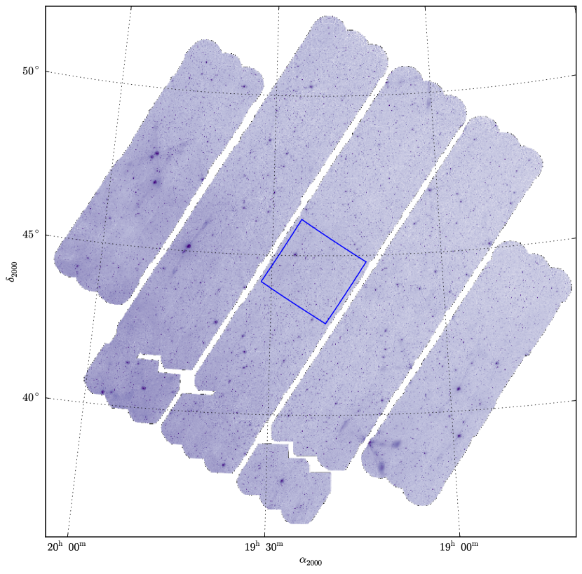
Figure 2.— Intensity image mosaic of GALEX CAUSE NUV observations. The blue square corresponds to the central CCD of the Kepler telescope.

Table 1Files of GCK dataset

Fits name	Image type	Units
nd-count.fits	count image	photons/pix
nd-rrhr.fits	effective exposure map	seconds/pix
nd-int.fits	intensity map	photons/second/pix
nd-flags.fits	artifact flags image	..
xd-mcat.fits	catalog of sources	..

The GCK data were processed with the GALEX scan-mode pipeline and subsequently delivered to Cornell in the form of packs of 5 images (see Table 1 for details) per visit for each tile. For details on these files or any technical information concerning the GALEX mission see: http://www.galex.caltech.edu/wiki/Public:Documentation.

A mosaic of the GALEX CAUSE NUV observations is shown on Fig. 2. The superimposed blue box corresponds to the central CCD of the Kepler detector array. Most of the data exhibit the exquisite photometric and astrometric stability and reproducibility expected for a space observatory. However, the GALEX pipeline failed to correctly process a small fraction of the images. A thorough visual inspection showed that there are about 450 images affected by doubling or ghosting of sources. An example of this effect is illustrated in Fig. 3. All these images were excluded from our analysis.

The final exposure time map is presented in Fig. 4. Some tiles lack a single good visit and are located at the end of a scan, when the spacecraft was executing a maneuver. Because of this, the 13th image of scans 4, 5, 6, 9 and 10 were not included in the catalog construction (leaving a total of 175 tiles), representing a loss of no more than 0.5% coverage of the Kepler field. Within the main GALEX  surveys, fractions of the Kepler field were partially surveyed (Smith et al., 2011). A cumulative distribution of the exposure time in function of sky coverage is shown in Fig. 5 (solid blue line), and the orange dashed line corresponds to the GALEX release 6 (GR6).

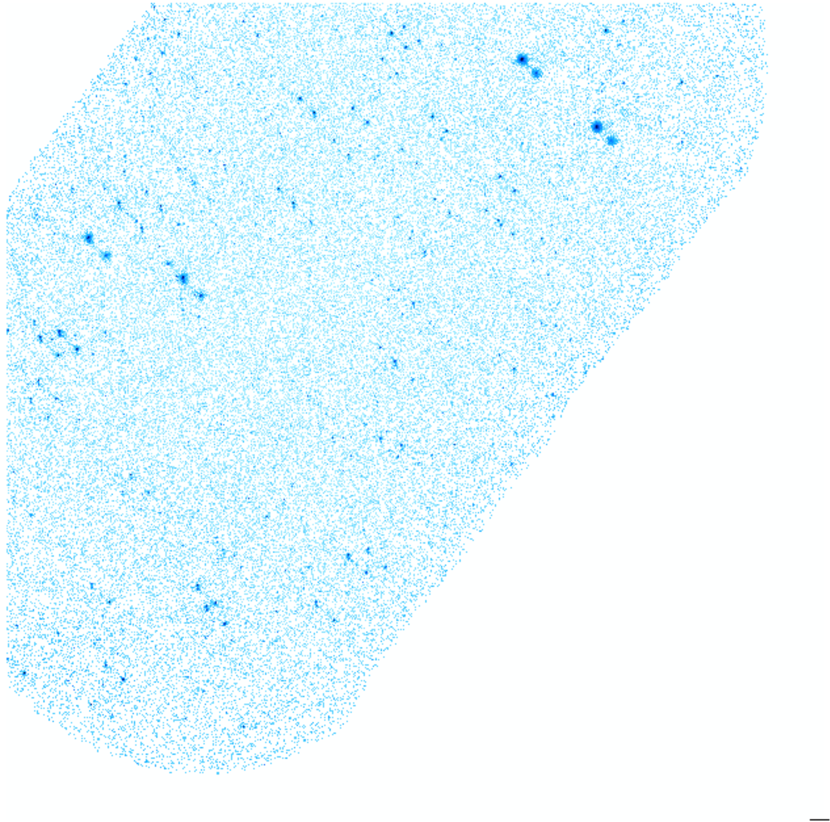
Figure 3.— GALEX image corresponding to scan 1, image 2, visit 2, as an example of a failure of the pipeline processing: bright sources appear as double objects.

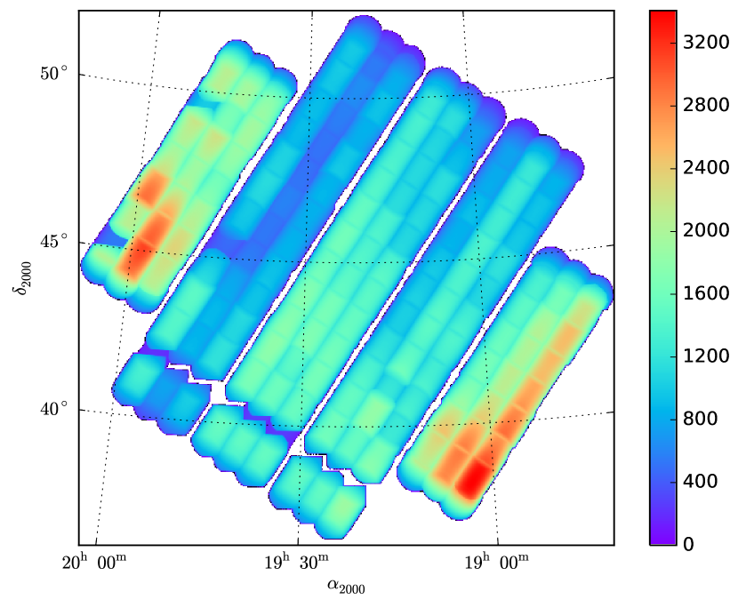
Figure 4.— Mosaic of the effective exposure time of the GALEX CAUSE observations.

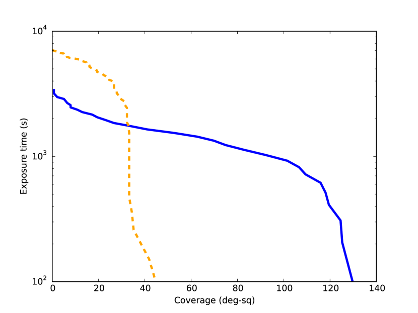
Figure 5.— Cumulative distributions of exposure time of the sky coverage of the GCK Kepler field (solid blue line). Observations from the GALEX release 6 (GR6) are represented with the dashed orange line.

III. Assembly of a Catalogue of NUV Sources

The construction of the GCK catalog can be summarised in 4 stages, each of which is discussed in this section. In the first stage, ”Image Co-adding”, the available single epoch visits for each tile are co-added. Next, the ”Background Estimation” is carried out from the intensity image using a modified $\sigma$-$\kappa$ clipping method. The ”Source Extraction and Photometry” uses the software SExtractor (Bertin & Arnouts, 1996) to first detect and then perform photometry on the background-subtracted intensity image for each tile obtained in the previous stage. In the final stage the catalogs from each of the 175 tiles are combined, and duplicate objects, low S/N sources, and other possible spurious sources are carefully removed.

III.1. Image Co-adding

Prior to co-adding all epochs for a given tile, each image was visually inspected, discarding visits presenting the source doubling or ghosting issue (Fig. 3). Since the images already have an astrometric solution, and furthermore, each epoch for a given tile are aligned, co-adding only requires an arithmetic sum. For each tile, the process was the following:

1. Construction of the co-added count image as the arithmetic sum of individual count intensity images (nd-count.fits).

2. Construction of the co-added effective exposure image as the arithmetic sum of individual effective exposure images (nd-rrhr.fits).

3. Construction of a combined flag image as the logic OR of the individual flag images (nd-flags.fits).

4. Calculation of the the ratio of the co-added count and effective exposure images to obtain the final intensity image.

III.2. Background and Threshold Estimations

The source extraction and photometry methodology follows that of the GALEX pipeline (reported in Morrissey et al., 2007). Prior to this step, background and threshold images are built, as required by SExtractor.

Background estimation: the construction of a background image consists of an iterative $\sigma$-$\kappa$ clipping method. The count image is divided into square bins 128 pix wide. In each bin, the local background histogram is built using the Poisson distribution (due to the low NUV background count rates), and the probability ${P_{k}}(x)$ of observing $k$ events for a mean rate $x$ is calculated. Pixels with a ${P_{k}}(x)<1.35\times{10^{-3}}$ (equivalent to a $3\sigma$ level) are iteratively clipped until convergence is reached. Then a $5\times 5$ pix median filter is applied to decrease the bias by bright sources. The bin mesh is upsampled to the original resolution and divided by the effective exposure image to produce the final background image, which is subtracted from the intensity image to produce the background-subtracted intensity image.

Weight threshold image: this image provides the threshold for potential detections. The count image is again divided in 128$\times$128 pix bins. In each bin the value of $k$, in counts/pix, which corresponds to probability level of $3\sigma$ is computed and stored to produce a threshold map. This map is upsampled to the original resolution and divided by the effective exposure image, in order to obtain a threshold image in counts/sec/pix. The final step is to compute a weight threshold image by dividing the background-subtracted intensity image by this last threshold image.

III.3. Source Extraction and Photometry

The detection and photometry process is carried out with SExtractor working in dual mode: the weight threshold image is used for detecting sources, while their photometry is computed on the background-subtracted intensity image. The SExtractor parameters THRESH_TYPE and DETECT_THRESH are set to ”absolute” and ”1”; in this way SExtractor will consider all pixels with values above 1 in the weight threshold image as possible detections. SExtractor is executed for each of the 175 tiles in the GCK data, delivering detection and photometry of each source. The photometric error $dm$ in magnitude is calculated following the GALEX pipeline:

$$df={{\sqrt{(f+s\Omega)t}}\over t},\;\;\;\;dm=1.086\cdot df/f,$$ (1)

where $f$ is the flux from the source in counts/sec, $s$ is the sky level in counts/sec/pix, $\Omega$ is the area over which the flux is measured and $t$ is the effective exposure time in seconds.

III.4. Artifact Identification

In the GALEX imagery, there are various artifacts, not all of which are automatically detected by the GALEX pipeline. The worrisome non-flagged artifacts are large diffuse reflections within the field surrounding very bright stars. The shapes of these artifacts have quite different morphologies, however the most common shapes are long thin cones, halos, and horseshoe-shaped extended reflections. An example is shown in Fig. 6. These artifacts bias the background and affect source detection, mainly producing false positives.

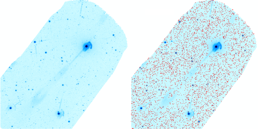
Figure 6.— Left panel: Co-added intensity image for image 6 of scan 2. Right panel: the same image with source detected marked as red points. Note the absence of detection in the area affected by instrumental artifacts.

III.4.1 False Positives

In order to remove extended objects and spurious detections, caused by non-flagged artifacts in the images, we design suitable criteria to remove them, while at the same time minimizing the loss of genuine sources. The criteria were defined considering the geometric characteristics of the aperture fitted by SExtractor to the flux profile of detection and the signal-to-noise ratio (S/N):

• Semi-minor axis $>$ 60″

• Eccentricity $>$ 0.95

• S/N $<$ 1.05

• S/N $<$ 1.5 & Semi-major axis $>$ 10″.

The first two criteria are intended to remove large and/or extended sources, including false detections inside extended artifacts. The third criteria discards too low S/N detections, while the purpose of the fourth criteria is to remove detections at the border of images, where the flux inside the SExtractor apertures may not be reliable. We defined the above thresholds through a trial and error process, aimed at discarding most of the false positives, while minimizing the loss of real sourcesones. The right panel of Fig. 6 shows the source detections after removing false positives.

III.4.2 Artifact Flags

The GALEX pipeline produces a flag image for each tile. This image marks the pixels where the intensity image is affected by some artifacts or where artifacts were removed. Each detected source has the artifact_flags keyword, that is a logical OR of the artifact flags for pixels that were used to compute its photometry. These flags are summarized in Table 2. The flags were developed for the dither mode observations and in some cases are not directly applicable to the scan mode observations. For example, in dither mode observations, only the outer region of any field is close to the detector edge, but in scan mode the detector edge crosses nearly the entire field for a fraction (but only a fraction) of the integration. The detector edge proximity flag (Flag 6) is therefore set by the pipeline, but it does not induce errors in the data quality. Flags 1 and 5 indicate the possible presence of reflections near the edge of the FOV. However, we have found that in many instances the regions affected by this latter artifact do not actually show any obvious problem. We therefore consider Flag 1 and 5 as non influential. Detections with flags 2, 3, and 10 have been discarded because their photometry is affected by an unreliable background level determination. An example of an image which presents regions marked by the flag 3, the dichroic reflection, is shown in Fig. 6, where one can distinguish arc-shaped features around the three brightest stars in the image.

The GALEX pipeline flags were developed for the dither mode observations and in some cases are not directly applicable to the scan mode observations in the same way as the dither mode observations. For example, in dither mode only the outer region of any field is close to the detector edge, but in scan mode the detector edge crosses nearly the entire field for a fraction (but only a fraction) of the integration. The detector edge proximity flag is therefore set by the pipeline, but it does not induce errors in the data quality

Table 2Artifact Flags

Number	Short name	Description
1(1)	edge	Detector bevel edge reflection (NUV only)
2(2)	window	Detector window reflection (NUV only)
3(4)	dichroic	Dichroic reflection
4(8)	varpix	Variable pixel based on time slices
5(16)	brtedge	Bright star near field edge (NUV only)
6(32)	detector rim	Proximity($>$0.6 degrees from field center)
7(64)	dimask	Dichroic reflection artifact mask flag
8(128)	varmask	Masked pixel determined by varpix
9(256)	hotmask	Detector hot spots
10(512)	yaghost	Possible ghost image from YA slope

Note. — From the GALEX documentation, chapter 8 (http://www.galex.caltech.edu/wiki/Public:Documentation/Chapter_8). Artifacts 7, 8, 9 do not apply to the the GCK catalog.

IV. The GCK UV source catalog

After processing each file through false positive removal and flagging, the 175 catalogs are combined to produce a single point source catalog for the whole GCK field. In the case of sources with multiple detections (due to small overlap between tiles), the measurement with the highest S/N was retained.

The resulting GCK catalog contains 660,928 NUV sources. The NUV brightness distribution of the GCK sources is shown in Fig. 7 (blue lines), while the photometric error is plotted in Fig. 8. One can see that a typical error for sources with NUV$<$22.6 mag is less than 0.3 mag.

The GCK Catalog includes a few thousand objects with NUV$\lesssim$15.5, whose flux estimation is affected by the non-linearity of the GALEX NUV detector (discussed by Morrissey et al., 2007). The magnitude of this non-linearity effect can be as large as $\sim$1.0 mag at NUV $\simeq$ 12 mag. In a recent analysis of the GALEX absolute calibration, Camarota & Holberg (2014) identified a non-linear correlation when comparing GALEX data of an extend sample of white dwarf stars with predicted magnitudes from model atmospheres and spectroscopic data collected by the International Ultraviolet Explorer (IUE). They provide a correction that properly converts the GALEX NUV magnitudes to the Hubble Space Telescope photometric scale. We applied this correction, based on the data in Table 3 of Camarota & Holberg (2014), to all GCK stars with NUV$\leq$15.71 mag, for which we also provide the original GALEX magnitudes. We also obtain an uncertainty of 0.22 mag, associated to the magnitude conversion, by computing the standard deviation of the Camarota & Holberg (2014) data with respect to their best fit.

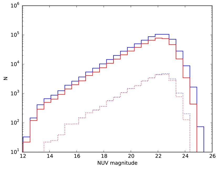
Figure 7.— Distribution of NUV detections. Blue line is the distribution of objects on the GCK catalog, red line are the matched objects with the KIC. Dotted lines correspond to a sample of detections inside a the sky region defined on Figure  2.

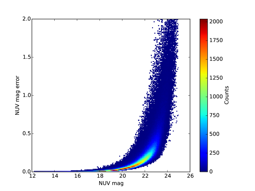
Figure 8.— NUV photometric error distribution for the GCK catalog. The color scale indicates the density of the sources in the plot.

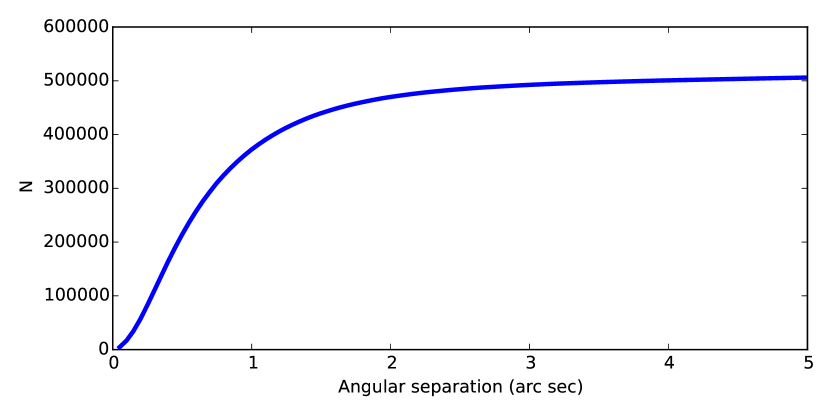
Figure 9.— Cumulative distributions of separations of the GCK - KIC cross-match.

V. Crossmatch with KIC and KOI

The positions of the GCK objects were cross-matched with the KIC (Brown et al., 2011), using a 2″.5 search radius. This value is compatible with the astrometric precision of GALEX observations, extending the crossmatch beyond this radius do not increase the number of matches more than 1%, as can be seen in the Fig. 9. The cross-match resulted in 475,164 GCK objects with KIC counterparts. We would like to remark that a smaller search radius would significantly decrease the number of detections, while a larger radius would only increase the KIC sources to be associated with a single NUV source. In the final catalogue we provide the identification of KIC counterparts.

The spatial location of these objects are plotted as red points in Fig. 10, where they obviously coincide with the position of the Kepler satellite detectors. Their NUV brightness distribution is also shown in Fig. 7. The constant ratio difference (up to NUV$\sim$22.5 mag) between GCK and KIC distributions seen in Fig. 7 is due to incomplete coverage of the Kepler field (caused by the gaps between the Kepler mission detectors (Fig. 10). In order to avoid this issue, we also show in Fig. 7 the number distribution of GCK sources and their KIC counterparts of the objects on the central Kepler detector(see Fig. 2); we can see that almost all GCK sources have KIC counterparts up to NUV$\sim$22.5 mag.

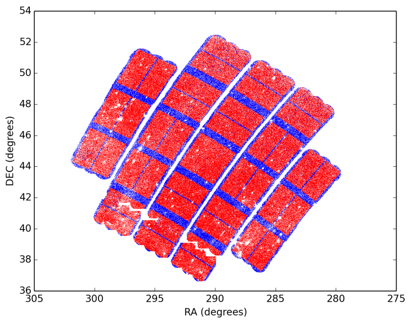
Figure 10.— Spatial distribution of the GCK sources in the Kepler field. Red dots indicate GCK sources with a counterpart in the KIC, while blue dots mark GKC sources without a KIC match. The saw-like regions in the south-east show the tile that were lost due to the pipeline failure (see Sect. II). Small circular empty regions are due to very bright stars, whose surrounding artifacts compromised nearby sources detections.

We also cross-matched the GCK catalog with the KOI catalog available in MAST through the tool CasJobs, and found 2614 candidate host stars (hosting 3390 planets) in common and 327 stars (hosting 768 planets) among the Kepler Confirmed Planets hosts. The GCK catalog should enable investigation of the UV excess as a function of stellar age, rotation, and metallicity, identification of UV-bright (potentially young) stars, and provide UV photometry for other astrophysically interesting systems in the Kepler field.

VI. Description of the catalog file

Table 3 provides the description of the fields in the GCK catalog file (columns 1 to 19). The first keyword is the gck_id, the main identifier of the GCK catalog, with a sexagesimal, equatorial position-based source name (i.e. GCK Jhhmmss.ss$+$ddmmss.s). The second and third keywords are the coordinates of the NUV detection. The following keywords give the photometry in magnitudes and fluxes, with their corresponding errors. The keyword artifacts_flags provides the flags described in Table 2. For objects with a cross-match in the KIC the keywords ktswckey and kic_keplerid, are provided for the nearest counterpart. The keyword ktswckey is particularly useful to get data from the table keplerObjectSearchWithColors, also available in MAST through the tool CasJobs. This table contains the KIC catalog and other catalogs with coverage of the Kepler field. In Table 4, we show a portion of the GCK catalog. The column tags designates the keyword number that also appear in Table 3. The GCK catalog is approximately $\sim$150 Mb (in ASCII format) and the table is available electronically with this paper.

As a useful reference for readers Table 5 provides 323 sources identified in the crossmatch between the GCK catalog and the Kepler targets with confirmed planetary companions. A segment of this table is illustrated in Table 5 and contains the information of columns 1-7, 10, 17, 20-28 listed in Table 3.

Table 3GCK catalog tags

Tag Number	Tag Name	Description	Unit
1	gck_id	GALEX CAUSE Kepler (GCK) Identifier	number
2	alpha_j2000	Right ascension	Decimal degrees
3	delta_j2000	Declination	Decimal degrees
4	nuv_mag	Calibrated NUV magnitude	AB magnitude
5	nuv_magerr	Error of the calibrated NUV magnitude	AB magnitude
6	nuv_mag_cor	Corrected calibrated NUV magnitude with Camarota & Holberg (2014) calibration	AB magnitude
7	nuv_magerr_cor	Error of the corrected calibrated NUV magnitude	AB magnitude
8	nuv_flux	NUV flux	counts/sec
9	nuv_fluxerr	Error of NUV flux	counts/sec
10	nuv_s2n	Signal-to-noise ratio of NUV flux	dimensionless
11	nuv_bkgrnd_mag	NUV background surface brightness at source position	AB magnitude
12	nuv_bkgrnd_flux	Background NUV flux at source position	counts/sec/arcsec2
13	nuv_exptime	Effective exposure time at source position	seconds
14	fov_radius	Distance of source from center of tile	degrees
15	artifact_flags	Logical OR of artifact flags	number
16	ktswckey	Sequential number in CasJobs Kepler Colors Table of match	number
17	kic_keplerid	Kepler Input Catalog identifier of match	number
18	scan	GCK scan number	dimensionless
19	image	GCK image number	dimensionless
20	kep_name	Kepler host star name	dimensionless
21	kic_kepmag	Kepler-band magnitude	AB magnitude
22	kic_g	g-band Sloan magnitude from the Kepler Input Catalog	AB magnitude
23	kic_r	r-band Sloan magnitude from the Kepler Input Catalog	AB magnitude
24	kic_i	i-band Sloan magnitude from the Kepler Input Catalog	AB magnitude
25	kic_z	z-band Sloan magnitude from the Kepler Input Catalog	AB magnitude
26	twomass_j	2MASS J-band magnitude	Vega magnitude
27	twomass_h	2MASS H-band magnitude	Vega magnitude
28	twomass_k	2MASS K-band magnitude	Vega magnitude

Table 4GCK catalog sample

								Column
(1)	(2)	(3)	(4)	(5)	(6)	(7)	(8)	(9)	(10)	(11)	(12)	(13)	(14)	(15)	(16)	(17)	(18)	(19)
GCK J18461428+4420359	281.55948	44.34330	23.768	0.638	-999	-999	0.033	0.02	1.7	26.95	0.002	1013.0	0.843	32	792984	8344414	2	2
GCK J19531681+4926274	298.32004	49.44096	20.854	0.072	-999	-999	0.490	0.03	15.1	26.15	0.004	1262.5	0.754	32	None	None	15	4
GCK J19325850+4922011	293.24375	49.36697	20.038	0.055	-999	-999	1.040	0.05	19.8	26.60	0.002	692.6	0.497	17	None	None	12	5
GCK J19432870+3909313	295.86958	39.15869	14.803	0.003	14.681	0.220	129.076	0.35	366.7	25.79	0.005	1101.0	0.661	48	658168	4075067	9	14
GCK J19183283+3827439	289.63681	38.46219	22.907	0.285	-999	-999	0.074	0.02	3.8	26.34	0.003	1524.7	0.596	1	12145669	None	4	12
GCK J19145926+4453507	288.74693	44.89742	22.893	0.369	-999	-999	0.075	0.03	2.9	26.52	0.003	1372.3	0.197	4	4369546	8681571	7	7
GCK J19503417+4804597	297.64238	48.08325	22.789	0.251	-999	-999	0.083	0.02	4.3	26.01	0.004	1593.2	0.625	32	15256924	None	14	5
GCK J19290783+4543284	292.28261	45.72457	20.826	0.093	-999	-999	0.503	0.04	11.7	26.48	0.003	611.5	0.657	32	None	None	10	7
GCK J19550979+4151533	298.79079	41.86481	19.239	0.037	-999	-999	2.170	0.07	29.3	25.64	0.006	875.6	0.739	32	6369109	6469387	12	14
GCK J19523858+4422221	298.16074	44.37282	16.702	0.006	-999	-999	22.440	0.12	193.2	25.98	0.004	1819.6	0.415	20	14957236	None	13	8

Note. — Column number correspond to tag number in Table 3. A -999 value indicates a non available data.

Table 5NUV magnitudes and ancillary data for Kepler targets with confirmed exoplanets

								Column
(17)	(20)	(1)	(2)	(3)	(4)	(5)	(6)	(7)	(10)	(21)	(22)	(23)	(24)	(25)	(26)	(27)	(28)
8359498	Kepler-77	GCK J19182585+4420438	289.60772	44.34550	20.575	0.056	-999	-999	19.43	13.938	14.449	13.871	13.720	13.658	12.757	12.444	12.361
8644288	Kepler-18	GCK J19521905+4444474	298.07939	44.74650	20.842	0.062	-999	-999	17.62	13.549	14.160	13.479	13.287	13.187	12.189	11.872	11.756
6616218	Kepler-314	GCK J19384180+4204320	294.67418	42.07566	19.777	0.035	-999	-999	31.03	12.557	13.126	12.459	12.313	12.205	11.242	10.849	10.778
9821454	Kepler-59	GCK J19080950+4638249	287.03957	46.64025	19.263	0.026	-999	-999	41.77	14.307	14.669	14.259	14.152	14.116	13.253	12.974	12.928
9595827	Kepler-71	GCK J19392762+4617097	294.86508	46.28602	21.969	0.226	-999	-999	4.80	15.127	15.692	15.061	14.885	14.803	13.926	13.550	13.468
9884104	Kepler-219	GCK J19145734+4645455	288.73890	46.76264	19.609	0.031	-999	-999	35.27	13.764	14.174	13.692	13.588	13.537	12.678	12.400	12.388
11121752	Kepler-380	GCK J18493471+4845327	282.39464	48.75907	18.278	0.031	-999	-999	35.46	13.652	14.047	13.614	13.483	13.464	12.614	12.349	12.288
2302548	Kepler-261	GCK J19252754+3736322	291.36477	37.60894	21.181	0.143	-999	-999	7.58	13.562	14.271	13.495	13.259	13.118	12.127	11.672	11.585
8572936	Kepler-34	GCK J19454460+4438294	296.43583	44.64151	20.884	0.089	-999	-999	12.25	14.875	15.372	14.830	14.662	14.575	13.605	13.301	13.237
6850504	Kepler-20	GCK J19104751+4220188	287.69795	42.33856	18.900	0.019	-999	-999	56.16	12.498	12.997	12.423	12.284	12.209	11.252	10.910	10.871

Note. — Column number correspond to tag number in Table 3. A -999 value indicates an unavailable datum. Table 5 is available in its entirety online as a machine readable table.

References

- Basri et al. (2005) Basri, G., Borucki, W. J., & Koch, D. 2005, New A Rev., 49, 478
- Bertin & Arnouts (1996) Bertin, E., & Arnouts, S. 1996, A&AS, 117, 393
- Bianchi et al. (2014) Bianchi, L., Conti, A., & Shiao, B. 2014, Advances in Space Research, 53, 900
- Borucki et al. (2003) Borucki, W. J., Koch, D. G., Lissauer, J. J., et al. 2003, in Society of Photo-Optical Instrumentation Engineers (SPIE) Conference Series, Vol. 4854, Future EUV/UV and Visible Space Astrophysics Missions and Instrumentation., ed. J. C. Blades & O. H. W. Siegmund, 129–140
- Brown et al. (2005) Brown, T. M., Everett, M., Latham, D. W., & Monet, D. G. 2005, in Bulletin of the American Astronomical Society, Vol. 37, American Astronomical Society Meeting Abstracts, 110.12
- Brown et al. (2011) Brown, T. M., Latham, D. W., Everett, M. E., & Esquerdo, G. A. 2011, AJ, 142, 112
- Camarota & Holberg (2014) Camarota, L., & Holberg, J. B. 2014, MNRAS, 438, 3111
- do Nascimento et al. (2014) do Nascimento, Jr., J.-D., García, R. A., Mathur, S., et al. 2014, ApJ, 790, L23
- Everett et al. (2012) Everett, M. E., Howell, S. B., & Kinemuchi, K. 2012, PASP, 124, 316
- Findeisen et al. (2011) Findeisen, K., Hillenbrand, L., & Soderblom, D. 2011, AJ, 142, 23
- García et al. (2014) García, R. A., Ceillier, T., Salabert, D., et al. 2014, A&A, 572, A34
- Greiss et al. (2012) Greiss, S., Steeghs, D., Gänsicke, B. T., et al. 2012, AJ, 144, 24
- Kawaler (1988) Kawaler, S. D. 1988, ApJ, 333, 236
- Latham et al. (2005) Latham, D. W., Brown, T. M., Monet, D. G., et al. 2005, in Bulletin of the American Astronomical Society, Vol. 37, American Astronomical Society Meeting Abstracts, 110.13
- Lawrence et al. (2007) Lawrence, A., Warren, S. J., Almaini, O., et al. 2007, MNRAS, 379, 1599
- Mamajek & Hillenbrand (2008) Mamajek, E. E., & Hillenbrand, L. A. 2008, ApJ, 687, 1264
- Martin et al. (2005) Martin, D. C., Fanson, J., Schiminovich, D., et al. 2005, ApJ, 619, L1
- McQuillan et al. (2014) McQuillan, A., Mazeh, T., & Aigrain, S. 2014, ApJS, 211, 24
- Meibom et al. (2015) Meibom, S., Barnes, S. A., Platais, I., et al. 2015, ArXiv e-prints, arXiv:1501.05651
- Mestel (1968) Mestel, L. 1968, MNRAS, 138, 359
- Morrissey et al. (2007) Morrissey, P., Conrow, T., Barlow, T. A., et al. 2007, ApJS, 173, 682
- Narain & Ulmschneider (1996) Narain, U., & Ulmschneider, P. 1996, Space Sci. Rev., 75, 453
- Olmedo et al. (2013) Olmedo, M., Chávez, M., Bertone, E., & De la Luz, V. 2013, PASP, 125, 1436
- Reinhold et al. (2013) Reinhold, T., Reiners, A., & Basri, G. 2013, A&A, 560, A4
- Smith et al. (2011) Smith, M., Shiao, B., & Kepler. 2011, in Bulletin of the American Astronomical Society, Vol. 43, American Astronomical Society Meeting Abstracts 217, 140.16
- Ulmschneider & Musielak (2003) Ulmschneider, P., & Musielak, Z. 2003, in Astronomical Society of the Pacific Conference Series, Vol. 286, Current Theoretical Models and Future High Resolution Solar Observations: Preparing for ATST, ed. A. A. Pevtsov & H. Uitenbroek, 363
- Walkowicz & Basri (2013) Walkowicz, L. M., & Basri, G. S. 2013, MNRAS, 436, 1883