Nonlinear organic plasmonics

Abstract

Purely organic materials with negative and near-zero dielectric permittivity can be easily fabricated. Here we develop a theory of nonlinear non-steady-state organic plasmonics with strong laser pulses. The bistability response of the electron-vibrational model of organic materials in the condensed phase has been demonstrated. Non-steady-state organic plasmonics enable us to obtain near-zero dielectric permittivity during a short time. We have proposed to use non-steady-state organic plasmonics for the enhancement of intersite dipolar energy-transfer interaction in the quantum dot wire that influences on electron transport through nanojunctions. Such interactions can compensate Coulomb repulsions for particular conditions. We propose the exciton control of Coulomb blocking in the quantum dot wire based on the non-steady-state near-zero dielectric permittivity of the organic host medium.

I Introduction

Metallic inclusions in metamaterials are sources of strong absorption loss. This hinders many applications of metamaterials and plasmonics and motivates to search for efficient solutions to the loss problem [1]. Highly doped semiconductors [1,2] and doped graphene [3-5] can in principle solve the loss problem. However, the plasmonic frequency in these materials is an order of magnitude lower than that in metals making former most useful at mid-IR and THz regions. In this relation the question arises whether metal-free metamaterials and plasmonic systems, which do not suffer from excessive damping loss, can be realized in the visible range? With no doubts, inexpensive materials with such advanced properties can impact whole technological fields of nanoplasmonics and metamaterials.

Recently Noginov et al. showed that purely organic materials characterized by low losses with negative, near-zero, and smaller than unity dielectric permittivities can be easily fabricated, and propagation of a surface plasmon polariton at the material/air interface was demonstrated [6]. And even non-steady-state organic plasmonics with strong laser pulses may be realized [7] that can enable us to obtain near-zero dielectric permittivity during a short time only.

Approach [6] was explained in simple terms of the Lorentz model for linear spectra of dielectric permittivities of thin film dyes. However, the experiments with strong laser pulses [7] challenge theory.

Here we develop a theory of nonlinear non-steady-state organic plasmonics with strong laser pulse excitation. Our consideration is based on the model of the interaction of strong (phase modulated) laser pulse with organic molecules, Ref.[8], extended to the dipole-dipole intermolecular interactions in the condensed matter. We demonstrate the bistability response of organic materials in the condensed phase. We also propose the exciton control of Coulomb blocking [9] in the quantum dot wire based on the non-steady-state near-zero dielectric permittivity of the organic host medium using chirped laser pulses.

II Model and basic equations

In this section we shall extend our picture of ”moving” potentials of Ref.[8] to a condensed matter. In this picture we considered a molecule with two electronic states $n=1$ (ground) and $2$ (excited) in a solvent. The molecule is affected by a (phase modulated) pulse $\mathbf{E}(t)$

$$\mathbf{E}(t)=\frac{1}{2}\mathbf{e}\mathcal{E}(t)\exp(-i\omega t+i\varphi(t))+\mathrm{c.c.}\text{ \ \ }$$ (1)

the frequency of which is close to that of the transition $1\rightarrow 2$. Here $\mathcal{E}(t)$ and $\varphi(t)$ describe the change of the pulse amplitude and phase in time, $\mathbf{e}$ is unit polarization vectors, and the instantaneous pulse frequency is $\omega(t)=\omega-d\varphi(t)/dt$.

One can describe the influence of the vibrational subsystems of a molecule and a solvent on the electronic transition within the range of definite vibronic transition related to a high frequency optically active (OA) vibration as a modulation of this transition by low frequency (LF) OA vibrations $\{\omega_{s}\}$ [10-13]. Let us denote the disturbance of nuclear motion under electronic transition as $\alpha$. Electronic transition relaxation stimulated by LFOA vibrations is described by the correlation function $K(t)=\langle\alpha(0)\alpha(t)\rangle$ of the corresponding vibrational disturbance with characteristic attenuation time $\tau_{s}$ [14-23]. The analytic solution of the problem under consideration has been obtained due to the presence of a small parameter. For broad vibronic spectra satisfying the ”slow modulation” limit, we have $\sigma_{2s}\tau_{s}^{2}\gg 1$ where $\sigma_{2s}=K(0)$ is the LFOA vibration contribution to a second central moment of an absorption spectrum. According to Refs. [22,23], the following times are characteristic for the time evolution of the system under consideration: $\sigma_{2s}^{-1/2}<T^{\prime}<<\tau_{s}$, where $\sigma_{2s}^{-1/2}$ and $T^{\prime}=(\tau_{s}/\sigma_{2s})^{1/3}$ are the times of reversible and irreversible dephasing of the electronic transition, respectively. The characteristic frequency range of changing the optical transition probability can be evaluated as the inverse $T^{\prime}$, i.e. $(T^{\prime})^{-1}.$ Thus, one can consider $T^{\prime}$ as a time of the optical electronic transition. Therefore, the inequality $\tau_{s}\gg T^{\prime}$ implies that the optical transition is instantaneous. Thus, the condition $T^{\prime}/\tau_{s}<<1$ plays the role of a small parameter. This made it possible to describe vibrationally non-equilibrium populations in electronic states $1$ and $2$ by balance operator equations for the intense pulse excitation (pulse duration $t_{p}>T^{\prime}$). If the correlation function is exponential: $K(t)/K(0)\equiv S(t)=\exp(-|t|/\tau_{s})$, the balance operator equations transform into diffusional equations. Such a procedure has enabled us to solve the problem for strong pulses even with phase modulation [8,24,25].

Equations of Ref. [8] describing vibrationally non-equilibrium populations in electronic states $j=1,2$ for the intense chirped pulse excitation, extended to the dipole-dipole intermolecular interactions in the condensed matter (see Appendix), take the following form

$$\frac{\partial\rho_{jj}\left(\alpha,t\right)}{\partial t} = \frac{\left(-1\right)^{j}\pi}{2\hbar^{2}}\delta[\omega_{21}-p\Delta n-\omega\left(t\right)-\alpha]\left(\frac{\varepsilon_{b}+2}{3}\right)^{2}$$ (2)

$$\times|\mathbf{D}_{21}\mathcal{\vec{E}}(t)|^{2}\Delta^{\prime}\left(\alpha,t\right)+L_{jj}\rho_{jj}\left(\alpha,t\right)$$

where $\Delta^{\prime}\left(\alpha,t\right)=\rho_{11}\left(\alpha,t\right)-\rho_{22}\left(\alpha,t\right)$, $\Delta n=n_{1}-n_{2}$, $\mathbf{D}_{21}$ is the electronic matrix element of the dipole moment operator. Here $\rho_{jj}$ are the diagonal elements of the density matrix; $\omega_{21}$ is the frequency of Franck-Condon transition $1\rightarrow 2$, and the operator $L_{jj}$ describes the diffusion with respect to the coordinate $\alpha$ in the corresponding effective parabolic potential $U_{j}\left(\alpha\right)$

$$L_{jj}=\frac{1+\left(\alpha-\delta_{j2}\omega_{st}\right)\frac{\partial}{\partial\left(\alpha-\delta_{j2}\omega_{st}\right)}+\sigma_{2s}\frac{\partial^{2}}{\partial\left(\alpha-\delta_{j2}\omega_{st}\right)^{2}}}{\tau_{s}}$$ (3)

$\delta_{ij}$ is the Kronecker delta, $\omega_{st}$ is the Stokes shift of the equilibrium absorption and luminescence spectra. The partial density matrix of the system $\rho_{jj}\left(\alpha,t\right)$ describes the system distribution in states $1$ and $2$ with a given value of $\alpha$ at time $t$. The complete density matrix averaged over the stochastic process which modulates the system energy levels, is obtained by integration of $\rho_{jj}\left(\alpha,t\right)$ over $\alpha$, $\langle\rho\rangle_{jj}\left(t\right)=\int\rho_{jj}\left(\alpha,t\right)d\alpha$, where quantities $\langle\rho\rangle_{jj}\left(t\right)$ are nothing more nor less than the normalized populations of the corresponding electronic states: $\langle\rho\rangle_{jj}\left(t\right)\equiv n_{j}$, $n_{1}+n_{2}=1$. Furthermore, here $\varepsilon_{b}$ is the “bulk” relative permittivity (which can be due distant high-frequency resonances of the same absorbing molecules or a host medium), $p=\dfrac{4\pi}{3\hbar}|D_{12}|^{2}N$ is the strength of the near dipole-dipole interaction [26], $N$ is the density of molecules.

Knowing $\rho_{jj}\left(\alpha,t\right)$, one can calculate the susceptibility $\chi(\Omega,t)$ [8] that enables us to obtain the dielectric function $\varepsilon$ due to relation $\varepsilon(\Omega,t)=1+4\pi\chi(\Omega,t)$:

$$\varepsilon(\Omega,t) =1+ip_{12}\left(\frac{\varepsilon_{b}+2}{3}\right)\{\sqrt{\frac{\pi}{2\sigma_{2s}}}w[\frac{\Omega-(\omega_{21}-p\Delta n(t))}{\sqrt{2\sigma_{2s}}}]$$

$$-\pi\sigma_{a}\left(\frac{\varepsilon_{b}+2}{3}\right)^{2}\int_{0}^{t}dt^{\prime}\Delta^{\prime}\left(\omega_{21}-p\Delta n\left(t^{\prime}\right)-\omega\left(t^{\prime}\right),t^{\prime}\right)$$

$$\times\tilde{J}(t^{\prime})\sum_{j=1}^{2}\sqrt{\frac{\sigma_{2s}}{\sigma\left(t-t^{\prime}\right)}}w[\frac{\Omega+p\Delta n(t)-\omega_{j}\left(t,t^{\prime}\right)}{\sqrt{2\sigma\left(t-t^{\prime}\right)}}]\}$$ (4)

where $\tilde{J}\left(t\right)$ is the power density of the exciting radiation, $\sigma\left(t-t^{\prime}\right)=\sigma_{2s}\left[1-S^{2}\left(t-t^{\prime}\right)\right]$, $\omega_{j}\left(t,t^{\prime}\right)=\omega_{21}-\delta_{j2}\omega_{st}+[\omega\left(t^{\prime}\right)-\omega_{21}+p\Delta n\left(t^{\prime}\right)+\delta_{j2}\omega_{st}]S\left(t-t^{\prime}\right)$ are the first moments of the transient absorption ($j=1$) and the emission ($j=2$) spectra, $\omega_{st}=\hbar\sigma_{2s}/\left(k_{B}T\right)$ is the Stokes shift of the equilibrium absorption and luminescence spectra, and

$$w(z)=\exp(-z^{2})[1+i\frac{2}{\sqrt{\pi}}\int_{0}^{z}\exp(y^{2})dy]$$

is the probability integral of a complex argument [27]. It is worthy to note that magnitude $\varepsilon(\Omega,t)$ does make sense, since it changes in time slowly with respect to dephasing. In other words, $\varepsilon(\Omega,t)$ changes in time slowly with respect to the reciprocal characteristic frequency domain of changing $\varepsilon(\Omega)$.

II.1 Fast vibrational relaxation

Let us consider the particular case of fast vibrational relaxation when one can put the correlation function $S\left(t-t^{\prime}\right)$ equal to zero. Physically it means that the equilibrium distributions into the electronic states have had time to be set during changing the pulse parameters. Using Eq.(2), one can obtain the equations for the populations of electronic states $n_{1,2}$ in the case under consideration, which represents extending Eq.(25) of Ref.[8] to the interacting medium

$$\frac{dn_{1,2}}{dt} = \pm\sigma_{a}\left(\frac{\varepsilon_{b}+2}{3}\right)^{2}\exp\{-\frac{\left[\omega_{21}-p\Delta n-\omega\left(t\right)-\omega_{st}\right]}{2\sigma_{2s}}^{2}\}$$ (5)

$$\times\tilde{J}\{n_{2}-n_{1}\exp\left[\hbar\beta\left(\omega\left(t\right)+p\Delta n-\omega_{21}+\frac{\omega_{st}}{2}\right)\right]\}$$

$$\pm\frac{n_{2}}{T_{1}}$$

where $\beta=1/k_{B}T$, $n_{1}+n_{2}=1$, $\sigma_{a}$ is the cross section at the maximum of the absorption band, and we added term ”$\pm n_{2}/T_{1}$” taking the lifetime $T_{1}$ of the excited state into account.

In case of fast vibrational relaxation, Eq.(4) becomes

$$\varepsilon(\Omega,t) =1+ip_{12}\left(\frac{\varepsilon_{b}+2}{3}\right)\sqrt{\frac{\pi}{2\sigma_{2s}}}\times$$

$$\times\sum_{j=1,2}(-1)^{j+1}n_{j}\left(t\right)w[\frac{\Omega-\omega_{21}+p\Delta n(t)+\delta_{2j}\omega_{st}}{\sqrt{2\sigma_{2s}}}]$$ (6)

III Excitation by chirped pulses compensating ”local field” detuning

Eqs. (2) and even (5) for populations are nonlinear equations where the transition frequencies are the functions of the electronic states populations. So, their solution in general case is not a simple problem. However, one can use pulses that are suitably chirped (time-dependent carrier frequency) to compensate for a change of frequency of the optical transition in time induced by the pulses themselves. This idea was proposed in studies of a two-state system in relation to Rabi oscillations in inter-subband transitions in quantum wells [28] and for obtaining efficient stimulated Raman adiabatic passage (STIRAP) in molecules in a dense medium [29].

Let us assume that we use suitably chirped pulses compensating the ”local field” detuning $p\Delta n$ that enables us to keep the value of $\omega_{21}-p\Delta n\left(t\right)-\omega\left(t\right)\equiv\Delta\omega$ as a constant ($\Delta\omega=const$). In that case one can obtain an integral equation

$$\Delta\left(t\right) = 1-\sigma_{a}\left(\frac{\varepsilon_{b}+2}{3}\right)^{2}\int_{0}^{t}dt^{\prime}\frac{\tilde{J}(t^{\prime})\Delta\left(t^{\prime}\right)}{\sqrt{1-S^{2}\left(t-t^{\prime}\right)}}$$ (7)

$$\times\sum_{j=1}^{2}\exp[-\frac{\left(\Delta\omega-\delta_{j2}\omega_{st}\right)^{2}}{2\sigma_{2s}}\frac{1-S\left(t-t^{\prime}\right)}{1+S\left(t-t^{\prime}\right)}]$$

for the dimensionless non-equilibrium population difference $\Delta\left(t\right)\equiv\Delta^{\prime}\left(\Delta\omega,t\right)/\Delta^{\prime\left(0\right)}\left(\Delta\omega\right)$, the effective methods of the solution of which were developed in Refs. [8,25].

For fast vibrational relaxation, using Eq.(5), we get

$$\frac{dn_{1,2}}{dt} = \pm\sigma_{a}\left(\frac{\varepsilon_{b}+2}{3}\right)^{2}\tilde{J}(t)\exp(-\frac{\Delta\omega^{2}}{2\sigma_{2s}})\{n_{2}$$ (8)

$$\times\exp[-\frac{\hbar\beta}{2}(\omega_{st}-2\Delta\omega)]-n_{1}\}\pm\frac{n_{2}}{T_{1}}$$

III.1 Near-zero dielectric function of dense collection of molecules excited with laser pulse

In this section we shall use Eqs.(6) and (8) to demonstrate obtaining near-zero dielectric function in non-steady-state regime. We shall consider a dense collection of molecules ($N\sim 10^{21}cm^{-3}$ [6]) with parameters close to those of molecule LD690 [8]: $\sqrt{\sigma_{2s}}=546cm^{-1}$, $D_{12}\sim 10^{-17}$ CGSE that gives $\omega_{st}=1420cm^{-1}$, $p_{12}=\allowbreak 2107.\,\allowbreak 2cm^{-1}$. We shall put $\varepsilon_{b}=1$ [6] and $\Delta\omega=-420cm^{-1}$. Fig.1 shows the population of excited electronic state $n_{2}$ and the real $\varepsilon^{\prime}(\Omega,t)$ and imaginary $\varepsilon^{\prime\prime}(\Omega,t)$ parts of $\varepsilon(\Omega,t)$ for $\Omega-\omega_{21}=-2.\,\allowbreak 040\,5\sqrt{2\sigma_{2s}}$ during the action of a rectangular light pulse of power density $\tilde{J}$ that begins at $t=0$.

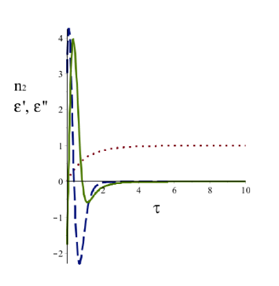
Figure 1: Population of the excited state (dots), and real (solid line) and imaginary (dashed line) parts of the dielectric function as functions of time.

Here we denoted

$$W=\sigma_{a}\left(\frac{\varepsilon_{b}+2}{3}\right)^{2}\exp(-\frac{\Delta\omega^{2}}{2\sigma_{2s}})\tilde{J}$$ (9)

- the probability of the optical transitions induced by external field, and $\tau=Wt$ - dimensionless time. We put $WT_{1}=1000$. Fig.1 illustrates non-steady-state near-zero dielectric permittivity. As population $n_{2}$ approaches to $1$, dielectric permittivity approaches to zero.

IV Application to exciton compensation of Coulomb blocking (ECCB) in conduction nanojunctions

In Ref. [9] we studied the influence of both exciton effects and Coulomb repulsion on current in nanojunctions. We showed that dipolar energy-transfer interactions between the sites in the wire can at high voltage compensate Coulomb blocking for particular relationships between their values. Although in free exciton systems dipolar interactions $J$ ($\lesssim 0.01-0.1eV$ [30]) are considerably smaller than on-site Coulomb interaction $U$ (characteristically $U\sim 1$ eV [31]) the former may still have strong effects under some circumstances, e.g. in the vicinity of metallic structures in or near the nanojunctions. In such cases dipolar interactions may be enhanced. The enhancement of the dipole-dipole interaction calculated using finite-difference time-domain simulation for the dimer of silver spheres, and within the quasistatic approximation for a single sphere, reached the value of $0.13$ eV for nanosphere-shaped metallic contacts [9] that was smaller than $U$. In addition, this enhancement was accompanied by metal induced damping of excitation energy.

In this section we show that purely organic materials characterized by low losses with near-zero dielectric permittivities will enable us easily to obtain $J\sim 1$ eV$\sim U$. We shall consider a nanojunction consisting of a two site quantum dot wire between two metal leads with applied voltage bias. The junction is found into organic material with dielectric permittivity $\varepsilon$. The quantum dots of the wire posses dipole moments $\mathbf{D}_{1}$ and $\mathbf{D}_{2}$. The point dipoles are positioned at points $\mathbf{r}_{1}$ and $\mathbf{r}_{2}$, respectively, and oscillate with frequency $\Omega$. The interaction energy between dipoles $1$ and $2$ can be written in a symmetrized form as $J_{12}+J_{21}$ where

$$J_{12} =-\frac{1}{2}\mathbf{D}_{1}\cdot\mathbf{E}_{2}(\mathbf{r}_{1},\Omega,t)$$ (10)

$$J_{21} =-\frac{1}{2}\mathbf{D}_{2}\cdot\mathbf{E}_{1}(\mathbf{r}_{2},\Omega,t)$$ (11)

$\mathbf{E}_{2}(\mathbf{r}_{1},\Omega,t)$ $\sim\mathbf{D}_{2}$ is the electric field at a point $\mathbf{r}_{1}$ induced by the dipole $\mathbf{D}_{2}$, etc.

The electric field is given by Coulomb’s law

$$\mathbf{E}(\mathbf{r},\Omega,t)=\frac{1}{\varepsilon(\Omega,t)}\int\rho_{i}(\mathbf{r}^{\prime})\frac{\mathbf{r-r}^{\prime}}{\left|\mathbf{r-r}^{\prime}\right|^{3}}d^{3}\mathbf{r}^{\prime}$$ (12)

that corresponds to the electrostatic approximation. Such extension of the electrostatic formula is possible due slow changes in time of $\varepsilon(\Omega,t)$ (see above). Here the external charge density $\rho_{i}(\mathbf{r}^{\prime})$ due to the presence of dipole $\mathbf{D}_{i}$ can be written as [32] $\rho_{i}(\mathbf{r}^{\prime})=-\mathbf{D}_{i}\cdot\mathbf{\nabla}_{\mathbf{r}^{\prime}}\delta(\mathbf{r}^{\prime}-\mathbf{r}_{i})$ (we consider a point dipole positioned at point $\mathbf{r}_{i}$). One can show that $U_{12}=U_{21}\equiv\frac{1}{2}\hbar J(\Omega,t)$. This can be expected from the reciprocity theorem [33], according to which the fields of two dipoles $\mathbf{D}_{1}$ and $\mathbf{D}_{2}$ at positions $\mathbf{r}_{1}$ and $\mathbf{r}_{2}$ and oscillating with the same frequency $\Omega$ are related as $\mathbf{D}_{1}\cdot\mathbf{E}_{2}(\mathbf{r}_{1},\Omega)=\mathbf{D}_{2}\cdot\mathbf{E}_{1}(\mathbf{r}_{2},\Omega)$. If the dipoles are oriented parallel to the symmetry axis of the junction Shishodia11, the dipole-dipole interaction is given by $J(\Omega,t)=J_{vac}/\varepsilon(\Omega,t)$ where $J_{vac}=-2D_{1}D_{2}\left|\mathbf{r}_{1}\mathbf{-r}_{2}\right|^{-3}$ is the dipole-dipole interaction in vacuum. The bottom of Fig.3 shows $J$ as a function of time for a medium with dielectric function given by Fig.1. Putting $D_{1}=D_{2}=25D$ and $\left|\mathbf{r}_{1}\mathbf{-r}_{2}\right|=5nm$, one gets $\left|J_{vac}\right|=0.006\,25eV$, and the value of $\left|J(\Omega,t)\right|=1.\,\allowbreak 660\,2eV$ for $\tau=10$.

IV.1 Calculation of current. Optical switches based on ECCB.

Let us calculate current through the two site quantum dot nanojunction described in the beginning of this section using approach of Ref. [9] where the dipole-dipole interaction between quantum dots of the wire is defined by $J(\Omega,t)=J_{vac}/\varepsilon(\Omega,t)$ (see above). The Hamiltonian of the wire, Eq.(3) of Ref. [9], contained both the energy

$$H_{exc-exc}=\hbar J(\Omega,t)b_{1}^{{\dagger}}b_{2}+H.c.$$ (13)

and electron transfer interactions written in the resonance approximation

$$H_{el-el}=-\sum_{f=g,e}\Delta_{f}(\hat{c}_{2f}^{{\dagger}}\hat{c}_{1f}+\hat{c}_{1f}^{{\dagger}}\hat{c}_{2f})$$ (14)

The operators $b_{m}^{{\dagger}}={c}_{me}^{{\dagger}}{c}_{mg}$ and $b_{m}={c}_{mg}^{{\dagger}}{c}_{me}$ are exciton creation and annihilation operators on the molecular sites $m=1,2$. The Hamiltonian of the Coulomb interactions is expressed as

$$H_{cou}=\dfrac{U}{2}\sum_{m=1,2}N_{m}(N_{m}-1)$$

with $N_{m}={n}_{mg}+{n}_{me}$. Since in the medium with near-zero dielectric permittivities both exciton-exciton interaction $J$ and on-site Coulomb interaction $U$ can achieve the value of about $1$ $eV$ (see above), we account and add the additional two off-resonance terms to $H_{exc-exc}$ and $H_{el-el}$ respectively, as

$$H_{non-exe-exe} =\hbar J(\Omega,t)b_{1}^{{\dagger}}b_{2}^{{\dagger}}+H.c.~{},$$ (15)

$$H_{non-el-el} =-\sum_{\begin{subarray}{c}f,f^{\prime}=g,e\\ f\neq f^{\prime}\end{subarray}}\Delta_{ff^{\prime}}(\hat{c}_{2f}^{{\dagger}}\hat{c}_{1f^{\prime}}+\hat{c}_{1f^{\prime}}^{{\dagger}}\hat{c}_{2f})$$ (16)

Eq. 15 is so called non-Heitler-London term [35] taking into account creation and annihilation for excitation simultaneously at two sites (quantum dots). In this relation the following question arises: ”does the effect of ECCB survive for such large values of $\hbar J\sim 1$ eV$\sim U$?”

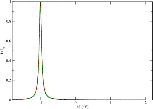
Figure 2: (Color online) Current $I/I_{0}$ displayed as function of the energy-transfer coupling $J$ for $U=1$ $eV$ and $\Delta_{f}=\Delta_{ff^{\prime}}\equiv\Delta=0.01eV$. The current shows a maximum at $U=-\hbar J$. Solid black line - calculations using Eqs.(13) and (14) for energy and electron transfer, respectively; red dashed line - calculations using Eqs.(13) and (15) for energy, and Eq.(14) for electron transfer; green dashed line - calculations using Eqs.(13) and (15) for energy, and Eqs.(14) and (16) for electron transfer. Comparison of these lines displays small effects of non-resonance contributions.

Fig.2 shows that the ECCB does survive for large values of $J\sim 1$ eV. We put the bias voltage $V_{bs}=8$ $eV$ and the rate of charge transfer from a quantum dot to the corresponding lead $\Gamma=0.02eV$ in our simulations, and denoted the unit of current as $I_{0}=\dfrac{e\Gamma}{\hbar}$ ($e$ is the charge of one electron). Fig.3 shows current through the nanojunction during the action of the rectangular lase pulse with parameters given in SectionIII.1 on the host organic material.

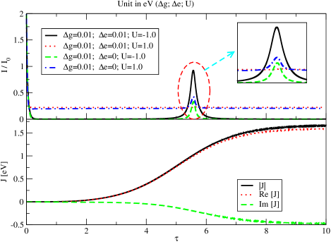
Figure 3: (Color online) Laser induced current $I/I_{0}$ (top) and the dipole-dipole interaction in an organic material $J[eV]$ (bottom) displayed as functions of $\tau$. Other parameters are identical to those of Fig.1.

One can see dramatic increasing the current when $\hbar J$ approaches to $-U$ for $\Delta_{g}=\Delta_{e}$, and to $\pm U$ for $\Delta_{g}\neq 0$ and $\Delta_{e}=0$. After this moment the current decreases in spite of increasing $J$, since its value exceeds that of $U$. So, current exists during the time that is much shorter than the pulse duration. As a matter of fact, Fig.3 illustrates a new type of optical switches based on the effect of the exciton compensation of Coulomb blocking - ECCB switches.

V Bistability

If one does not use suitably chirped pulses that compensate for a change of frequency of the optical transition in time induced by the pulses themselves (see SectionIII), Eqs. (2) and (5) for populations become nonlinear equations and can demonstrate a bistable behavior. Fig.4 shows steady-state solutions of Eq.(5) for $n_{2}$ as a function of the power density of the exciting radiation $\tilde{J}$ at different detunings $\omega_{21}-\omega$.

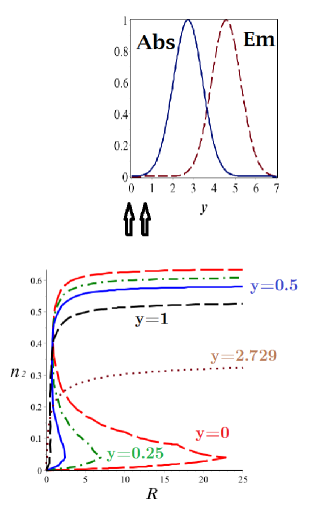
Figure 4: (Color online) Dependence of excited state population $n_{2}$ on power density of the exciting radiation $\tilde{J}$ at different detunings $\omega_{21}-\omega$. Dimensionless parameters are $R=\sigma_{a}\tilde{J}T_{1}$ and $y=(\omega_{21}-\omega)/\sqrt{2\sigma_{2s}}$. Parameters $\sqrt{\sigma_{2s}}$, $\omega_{st}$, $p_{12}$ and $\varepsilon_{b}$ are identical to those of SectionIII.1. Inset: Equilibrium spectra of the absorption (Abs) and the emission (Em); the arrows limit the frequency interval where calculated excited state populations $n_{2}$ show bistability.

One can see that each value of $\tilde{J}$ within the corresponding interval produces three different solutions of Eq.(5) for dimensionless detunings $y=(\omega_{21}-\omega)/\sqrt{2\sigma_{2s}}=0,$ $0.25$ and $0.5$, however, only lower and upper branches are stable [36]. Such detunings correspond to the excitation at the short-wave part of the equilibrium absorption spectrum (see the Inset to Fig.4). As the excited state population increases, the spectrum exhibits the blue shift (see Eq.(5) that should essentially contribute to the absorption. As a matter of fact, the bistable behavior of the population arises from the dependence of the resonance frequency of the molecules in dense medium on the number of excited molecules. In contrast, larger $y=1$, $2.729$ correspond to the excitation closer to the central part of the equilibrium absrption spectrum. In that case the blue shift produces lesser increasing the absorption and even can decrease it (for $y=2.729$), so that the bistable behavior disappears.

Furthermore, the excitation of surface plasmon polaritons at the organic thin film/air interface is possible for substantially strong negative values of dielectric function $\varepsilon(\Omega)$ [6,37].The bistable behavior of the population results in the bistable behavior of $\varepsilon(\Omega)$ (see Eqs.(4) and (6)), and as a consequence, a bistable behavior of the dispersion relations for surface plasmon polaritons at the organic thin film/air interface under the laser irradiation. This issue will be considered elsewhere.

VI Conclusion

In this work we have developed a theory of nonlinear non-steady-state organic plasmonics with strong laser pulses. We have demonstrated the bistabile response of the electron-vibrational model of organic materials in condensed phase that leads to the bistability of their plasmonic properties. Specifically, bistability in the regime of the surface plasmon polariton propagation at the organic thin film/air interface may be used for new types of optical switches. We have proposed to use non-steady-state organic plasmonics for the enhancement of intersite dipolar energy-transfer interaction in the quantum dot wire that influences on electron transport through nanojunctions. Such interactions can compensate Coulomb repulsions for particular conditions. We propose the exciton control of Coulomb blocking in the quantum dot wire based on the non-steady-state near-zero dielectric permittivity of the organic host medium, and a new type of optical switches - ECCB switches. Our current calculations were carried out for a value of $J(\Omega,t)$ corresponding to fixed frequency $\Omega$ $(=\omega_{21}-2.\,\allowbreak 040\,5\sqrt{2\sigma_{2s}})$. The extension of the calculations of current to frequency dependent $J(\Omega,t)$ will be made elsewhere.

VII Appendix

Let us generalize equations of Ref. [8] to the dipole-dipole intermolecular interactions in the condensed matter. The latter are described by Hamiltonian [18,35] $\hat{H}_{int}=\hbar\sum_{m\neq n}J_{mn}b_{m}^{{\dagger}}b_{n}+H.c.$ (compare with Eq.(13)). Using the Heisenberg equations of motion, one obtains that $\hat{H}_{int}$ gives the following contribution to the change of the expectation value of excitonic operator $b_{k}$ in time

$$\frac{d}{dt}\langle b_{k}\rangle \sim \frac{i}{\hbar}\langle[\hat{H}_{int},b_{k}]\rangle\equiv\frac{i}{\hbar}Tr([\hat{H}_{int},b_{k}]\rho)$$ (17)

$$= i2\sum\limits_{n\neq k}J_{kn}\langle(\hat{n}_{k2}-\hat{n}_{k1})b_{n}\rangle$$

where $\rho$ is the density matrix, $\left|k1\right\rangle\equiv\left|kg\right\rangle,$ $\left|k2\right\rangle\equiv\left|ke\right\rangle$, $\hat{n}_{k1}=b_{k}b_{k}^{{\dagger}}$, and $\hat{n}_{k2}=b_{k}^{{\dagger}}b_{k}$ is the exciton population operator. Considering an assembly of identical molecules, one can write $\langle b_{k}\rangle=\rho_{21}\left(\alpha,t\right)$ [29] if averaging in Eq.(17) is carried out using density matrix $\rho\left(\alpha,t\right)$. Consider the expectation value $\langle(\hat{n}_{k2}-\hat{n}_{k1})b_{n}\rangle=Tr[(\hat{n}_{k2}-\hat{n}_{k1})b_{n}\rho\left(\alpha,t\right)]$ for $n\neq k.$ Due to fast dephasing (see SectionII), it makes sense to neglect all correlations among different molecules [18], and set $\langle(\hat{n}_{k2}-\hat{n}_{k1})b_{n}\rangle=\langle\hat{n}_{k2}-\hat{n}_{k1}\rangle\langle b_{n}\rangle$. Here from dimension consideration one expectation value should be calculated using density matrix $\rho\left(\alpha,t\right)$, and another one - using $\langle\rho\rangle\left(t\right)=\int\rho\left(\alpha,t\right)d\alpha$. Bearing in mind fast dephasing, we choose option $\langle\hat{n}_{k2}-\hat{n}_{k1}\rangle\langle b_{n}\rangle=(n_{2}-n_{1})\rho_{21}\left(\alpha,t\right)$ that gives the most contribution and results in the agreement with experimental spectra of molecular thin films. Another option $\langle\hat{n}_{k2}-\hat{n}_{k1}\rangle\langle b_{n}\rangle=-\Delta^{\prime}\left(\alpha,t\right)\langle\rho\rangle_{21}\left(t\right)$ is more suitable to the creation of delocalized collective states, and similar to the procedure used for the derivation of the semiconductors Bloch equations [38,39].

It remains to calculate $2\sum_{n\neq k}J_{kn}=2\lim_{\mathbf{k}\rightarrow 0}J(\mathbf{k})$ on the right-hand side of Eq.(17) that is conveniently calculated in $\mathbf{k}$ space where $J(\mathbf{k})=\sum_{n\neq k}J_{kn}\exp(-i\mathbf{k}\cdot\mathbf{r}_{n})$, $\mathbf{r}_{n}$ denotes the position of the $n$th molecule. Bearing in mind that $\hbar J_{kn}\equiv\frac{1}{2}\mathbf{D}_{k}\cdot T_{kn}\cdot\mathbf{D}_{n}$ where $T_{kn}$ is the dipole-dipole tensor, and using $T(\mathbf{k})=-4\pi N/3$, Eq.(16.20b) of Ref. [18] for a transverse field (see also [40]), we get $2\sum_{n\neq k}J_{kn}=-p$. This yields $\partial\rho_{21}\left(\alpha,t\right)/\partial t\sim ip\Delta n\rho_{21}\left(\alpha,t\right)$. Adding term ”$ip\Delta n\rho_{21}\left(\alpha,t\right)$” to the right-hand side of Eq.(9) of Ref.[8], and using the procedure described there, we get Eq.(2).

References

[1] J. B. Khurgin, “How to deal with the loss in plasmonics and metamaterials,” Nature Nanotechnology, vol. 10, pp. 2–6, 2015.

[2] A. J. Hoffman, L. Alexeev, S. S. Howard, K. J. Franz, D. Wasserman, V. A. Podolskiy, E. E. Narimanov, D. L. Sivco, and C. Gmachl, “Negative refraction in semiconductor metamaterials,” Nature Materials, vol. 6, pp. 946–950, 2007.

[3] F. H. L. Koppens, D. E. Chang, and F. J. G. de Abajo, “Graphene plasmonics: A platform for strong light-matter interaction,” Nano Letters, vol. 11, pp. 3370–3377, 2011.

[4] J. Chen, M. Badioli, P. Alonso-Gonzalez, S. Thongrattanasiri, F. Huth, J. Osmond, M. Spasenovic, A. Centeno, A. Pesquera, P. Godignon, A. Z. Elorza, N. Camara, F. J. G. de Abajo, R. Hillenbrand, and F. H. L. Koppens, “Optical nano-imaging of gate-tunable graphene plasmons,” Nature, vol. 487, pp. 77–81, 2012.

[5] Z. Fei, A. S. Rodin, G. O. Andreev, W. Bao, A. S. McLeod, M. Wagner, L. M. Zhang, Z. Zhao, M. Thiemens, G. Dominguez, M. M. Fogler, A. H. C. Neto, C. N. Lau, F. Keilmann, and D. N. Basov, “Gate-tuning of graphene plasmons revealed by infrared nano-imagine,” Nature, vol. 487, pp. 82–85, 2012.

[6] L. Gu, J. Livenery, G. Zhu, E. E. Narimanov, and M. A. Noginov, “Quest for organic plasmonics,” Applied Phys. Lett., vol. 103, p. 021104, 2013.

[7] T. U. Tumkur, J. K. Kitur, L. Gu, G. Zhu, and M. A. Noginov, in Abstracts of NANOMETA 2013, Seefeld, Austria, 2013, p. FRI3o.6.

[8] B. D. Fainberg, “Nonperturbative analytic approach to interaction of intense ultrashort chirped pulses with molecules in solution: Picture of ”moving” potentials,” J. Chem. Phys., vol. 109, no. 11, pp. 4523–4532, 1998.

[9] G. Li, M. S. Shishodia, B. D. Fainberg, B. Apter, M. Oren, A. Nitzan, and M. Ratner, “Compensation of coulomb blocking and energy transfer in the current voltage characteristic of molecular conduction junctions,” Nano Letters, vol. 12, pp. 2228–2232, 2012.

[10] B. D. Fainberg and B. S. Neporent, Opt. Spectrosc., vol. 48, p. 393, 1980, [Opt. Spektrosk., v. 48, 712 (1980)].

[11] B. D. Fainberg and I. B. Neporent, Opt. Spectrosc., vol. 61, p. 31, 1986, [Opt. Spektrosk., v. 61, 48 (1986)].

[12] B. D. Fainberg and I. N. Myakisheva, Sov. J. Quant. Electron., vol. 17, p. 1595, 1987, [Kvantovaya Elektron. (Moscow), v. 14, 2509 (1987)].

[13] ——, Opt. Spectrosc., vol. 66, p. 591, 1989, [Opt. Spektrosk., v. 66, 1012 (1989)].

[14] B. D. Fainberg, Opt. Spectrosc., vol. 60, p. 74, 1986, [Opt. Spektrosk., v. 60, 120 (1986)].

[15] R. F. Loring, Y. J. Yan, and S. Mukamel, J. Chem. Phys., vol. 87, p. 5840, 1987.

[16] W. Vogel, D.-G. Welsh, and B. Wilhelmi, Phys. Rev. A, vol. 37, p. 3825, 1988.

[17] B. D. Fainberg, Opt. Spectrosc., vol. 65, p. 722, 1988, [Opt. Spektrosk., vol. 65, 1223, 1988].

[18] S. Mukamel, Principles of Nonlinear Optical Spectroscopy.   New York: Oxford University Press, 1995.

[19] V. V. Khizhnyakov, Izv. Akad. Nauk SSSR, Ser. Fiz., vol. 52, p. 765, 1988.

[20] B. D. Fainberg, Opt. Spectrosc., vol. 58, p. 323, 1985, [Opt. Spektrosk. v. 58, 533 (1985)].

[21] Y. J. Yan and S. Mukamel, Phys. Rev. A, vol. 41, p. 6485, 1990.

[22] B. D. Fainberg, Opt. Spectrosc., vol. 68, p. 305, 1990, [Opt. Spektrosk., vol. 68, 525, 1990].

[23] B. Fainberg, Phys. Rev. A, vol. 48, p. 849, 1993.

[24] B. D. Fainberg, Opt. Spectrosc., vol. 67, p. 137, 1989, [Opt. Spektrosk., v. 67, 241 (1989)].

[25] ——, “Non-linear polarization and spectroscopy of vibronic transitions in the field of intensive ultrashort pulses,” Chem. Phys., vol. 148, pp. 33–45, 1990.

[26] M. E. Crenshow, M. Scalora, and C. M. Bowden, “Ultrafast intrinsic optical switching in dense medium of two-level atoms,” Phys. Rev. Lett., vol. 68, pp. 911–914, 1992.

[27] M. Abramowitz and I. Stegun, Handbook on Mathematical Functions.   New York: Dover, 1964.

[28] A. A. Batista and D. S. Citrin, “Rabi flopping in a two-level system with a time-dependent energy renormalization: Intersubband transitions in quantum wells,” Phys. Rev. Lett., vol. 92, no. 12, p. 127404, 2004.

[29] B. D. Fainberg and B. Levinsky, “Stimulated raman adiabatic passage in a dense medium,” Adv. Phys. Chem., vol. 2010, p. 798419, 2010.

[30] S. Mukamel and D. Abramavicius, “Many-body approaches for simulating coherent nonlinear spectroscopies of electronic and vibrational excitons,” Chem. Rev., vol. 104, pp. 2073–2098, 2004.

[31] H. Thomann, L. R. Dalton, M. Grabowski, and T. C. Clarke, “Direct observation of coulomb correlation effects in polyacetylene,” Phys. Rev. B, vol. 31, no. 5, pp. 3141–3143, 1985.

[32] X. M. Hua, J. I. Gersten, and A. Nitzan, “Theory of energy transfer between molecules near solid particles,” J. Chem. Phys., vol. 83, no. 7, pp. 3650–3659, 1985.

[33] L. D. Landau and E. M. Lifshitz, Electrodynamics of Continuous Media.   New York: Pergamon Press, 1960.

[34] M. S. Shishodia, B. D. Fainberg, and A. Nitzan, “Theory of energy transfer interactions near sphere and nanoshell based plasmonic nanostructures,” in Plasmonics: Metallic Nanostructures and Their Optical Properties IX. Proc. of SPIE, M. I. Stockman, Ed.   Bellingham, WA: SPIE, 2011, vol. 8096, p. 8096 1G.

[35] A. S. Davydov, Theory of Molecular Excitons.   New York: Plenum, 1971.

[36] N. N. Bogoliubov and Y. A. Mitropolskyi, Asymptotic methods in the theory of non-linear oscillations.   New York: Gordon and Breach, 1961.

[37] H. Raether, Surface Plasmons on Smooth and Rough Surfaces and on Gratings.   Berlin: Springer-Verlag, 1986.

[38] M. Lindberg and S. W.Koch, “Effective bloch equations for semiconductors,” Phys. Rev. B, vol. 38, no. 5, pp. 3342–3350, 1988.

[39] H. Haug and S. W. Koch, Quantum theory of the optical and electronic properties of semiconductors.   Singapore: World Scientific, 2001.

[40] A. Gonzalez-Tudela, D. Martin-Cano, E. Moreno, L. Martin-Moreno, C. Tejedor, and F. J. Garcia-Vidal, “Dipolar sums in the primitive cubic lattices,” Phys.Rev., vol. 99, no. 4, pp. 1128–1134, 1955.