Measuring CP-Violating Observables
in Rare Top Decays at the LHC

Abstract

In this paper we consider CP-violating new-physics contributions to the decay $t\to b\bar{b}c$. We examine the prospects for detecting such new physics at the LHC, which requires studying the process $gg\to t(\to b\bar{b}c)\bar{t}(\to\bar{b}\ell\bar{\nu})$. We find two observables that can be used to reveal the presence of CP-violating new physics in $t\to b\bar{b}c$. They are (i) the partial-rate asymmetry and (ii) the triple-product correlations involving the momenta of various particles associated with the interaction. A Monte Carlo analysis is performed to determine how well these observables can be used to detect the presence of new physics, and to measure its parameters. We find that there is little difficulty in extracting the value of the relevant new-physics parameter from the partial-rate asymmetry. For the triple-product correlations, we test multiple strategies that can be used for the extraction of the corresponding combination of new-physics parameters.

I Introduction

It is widely believed that physics beyond the Standard Model (SM) must exist. However, to date, no evidence of this new physics (NP) has been found. It appears that the energy scale of the NP is larger than was hoped for, or that its manifestation is subtler than envisioned. Over the years many models of NP have been proposed, and a number of these feature the top quark in a central role topNPmodels . Being particularly heavy, with a mass near the electroweak scale, the top quark may well be sensitive to NP interactions that do not much affect other SM particles. On the other hand, top observables such as total cross-section topcsec , decay width topwidth , differential cross-sections topdifferential , etc. appear to be in good agreement with the corresponding SM predictions. Significant NP contributions may therefore exist only in processes that are suppressed in the SM. One such process is the decay $t\to b{\overline{b}}c$. The SM rate for this process is very small as it involves the Cabibbo-Kobayashi-Maskawa (CKM) element $V_{cb}$ ($\sim$ 0.04).

NP contributions to $t\to b{\overline{b}}c$ were studied in Ref. kklrsw , and several observables that can reveal the presence of NP were found. This decay can be studied at the LHC, which is essentially a top-quark factory. However, single-top production is rather suppressed at the LHC singletprod , so that it is difficult to isolate $t\to b{\overline{b}}c$ experimentally and analyze it on its own. Instead, one considers $t{\overline{t}}$ pairs that are produced predominantly through gluon fusion: $gg\to t{\overline{t}}$. The $t$ and ${\overline{t}}$ then decay into a pair of $b$-jets along with other hadronic and/or leptonic final states. In order to study $t\to b{\overline{b}}c$, it is useful to consider the semi-leptonic channel $gg\to t(\to b{\overline{b}}c){\overline{t}}(\to{\overline{b}}\ell{\overline{\nu}})$ where the charge of the lepton may be used to ascertain that it is the $t$ that is undergoing the rare decay.

In Refs. tNPLHC1 ; tNPLHC2 a detailed numerical simulation of $gg\to t(\to b{\overline{b}}c){\overline{t}}(\to{\overline{b}}\ell{\overline{\nu}})$ was performed to examine how well NP parameters can be determined at the LHC when it operates at 14 TeV. This analysis focused on CP-conserving NP. In the present paper, we examine the possibilities for detecting CP-violating NP and measuring its parameters. In Ref. kklrsw it was shown that there are two observables that are sensitive to CP violation in $t\to b{\overline{b}}c$ – the partial-rate asymmetry and the triple product. In the full process, $gg\to t(\to b{\overline{b}}c){\overline{t}}(\to{\overline{b}}\ell{\overline{\nu}})$, one has these same two observables. We examine each of these observables separately. For the partial-rate asymmetry, the analysis is straightforward. However, as we will see, for the triple product it is more involved.

We begin in Sec. II by describing the effective Lagrangian describing NP contributions to $t\to b{\overline{b}}c$ and outlining the calculation of the differential cross section for $gg\to t{\overline{t}}\to\left(b{\overline{b}}c\right)\left({\overline{b}}\ell{\overline{\nu}}\right)$. In Sec. III we define CP-violating observables in $gg\to t{\overline{t}}\to\left(b{\overline{b}}c\right)\left({\overline{b}}\ell{\overline{\nu}}\right)$. Included here are the analytic expressions for the partial-rate asymmetry and the triple product in this process. In Sec. IV we detail the numerical simulations performed to determine how well the CP-odd NP parameter combinations can be extracted from measurements of the partial-rate asymmetry, the triple product and related observables. We discuss the feasibility of measuring $gg\to t{\overline{t}}\to\left(b{\overline{b}}c\right)\left({\overline{b}}\ell{\overline{\nu}}\right)$ in Sec. V. We conclude in Sec. VI.

II New Physics Contributions to $t$ decay

II.1 $t\to b{\overline{b}}c$: effective Lagrangian

The decay $t\to b\overline{b}c$ can have contributions coming from the SM ($t\to bW^{+}\to b\overline{b}c$) and from various NP sources. We parameterize the NP contributions via an effective Lagrangian, as was done in Refs. kklrsw ; tNPLHC1 ; tNPLHC2 : we set ${\cal L}_{\mbox{\scriptsize eff}}={\cal L}_{\mbox{\scriptsize eff}}^{V}+{\cal L}_{\mbox{\scriptsize eff}}^{S}+{\cal L}_{\mbox{\scriptsize eff}}^{T}$, with

$${\cal L}_{\mbox{\scriptsize eff}}^{V} = 4\sqrt{2}G_{F}V_{cb}V_{tb}\left\{X_{LL}^{V}\,{\overline{b}}\gamma_{\mu}P_{L}t\,\overline{c}\gamma^{\mu}P_{L}b+X_{LR}^{V}\,{\overline{b}}\gamma_{\mu}P_{L}t\,\overline{c}\gamma^{\mu}P_{R}b\right.$$ (1)

$$\hskip 62.59596pt\left.+~{}X_{RL}^{V}\,{\overline{b}}\gamma_{\mu}P_{R}t\,\overline{c}\gamma^{\mu}P_{L}b+X_{RR}^{V}\,{\overline{b}}\gamma_{\mu}P_{R}t\,\overline{c}\gamma^{\mu}P_{R}b\right\}+\mbox{h.c.},$$

$${\cal L}_{\mbox{\scriptsize eff}}^{S} = 4\sqrt{2}G_{F}V_{cb}V_{tb}\left\{X_{LL}^{S}\,{\overline{b}}P_{L}t\,\overline{c}P_{L}b+X_{LR}^{S}\,{\overline{b}}P_{L}t\,\overline{c}P_{R}b\right.$$ (2)

$$\hskip 62.59596pt\left.+~{}X_{RL}^{S}\,{\overline{b}}P_{R}t\,\overline{c}P_{L}b+X_{RR}^{S}\,{\overline{b}}P_{R}t\,\overline{c}P_{R}b\right\}+\mbox{h.c.,}$$

$${\cal L}_{\mbox{\scriptsize eff}}^{T} = 4\sqrt{2}G_{F}V_{cb}V_{tb}\left\{X^{T}_{LL}\overline{b}\sigma^{\mu\nu}P_{L}t\,\overline{c}\sigma_{\mu\nu}P_{L}b\right.$$ (3)

$$\hskip 62.59596pt\left.+~{}X^{T}_{RR}{\overline{b}}\sigma^{\mu\nu}P_{R}t\,\overline{c}\sigma_{\mu\nu}P_{R}b\right\}+\mbox{h.c.}$$

The colour indices in the above expressions are assumed to contract in the same manner as those in the SM; Ref. kklrsw contains an analysis of the case in which the indices contract differently than in the SM.

The dimensionless NP parameters $X^{I}_{AB}$ in Eqs. (1)-(3) may be assumed to be $O(1)$. Under this assumption, the NP contributions to $t\to b\overline{b}c$ can be of the same order as that coming from the SM. For this reason, when analyzing possible NP effects it is important to consider not just the SM-NP interference terms, but also the NP-NP pieces. In this paper we focus specifically on CP-violating effects, which can arise when the $X^{I}_{AB}$ contain weak phases. Throughout this work we ignore strong phases related to NP contributions, since these are negligible DatLon . There is a strong phase related to the $W$ resonance in the SM contribution to the decay; this phase plays an important role in the partial-rate asymmetry (see Sec. III.1).

II.2 Differential cross section for $gg\to t{\overline{t}}\to\left(b{\overline{b}}c\right)\left({\overline{b}}\ell{\overline{\nu}}\right)$

The differential cross section for $gg\to t{\overline{t}}\to\left(b{\overline{b}}c\right)\left({\overline{b}}\ell{\overline{\nu}}\right)$ was worked out in Ref. tNPLHC1 . In this section we summarize the procedure; the results can be found in Appendix A. The full details are given in Ref. tNPLHC1 .

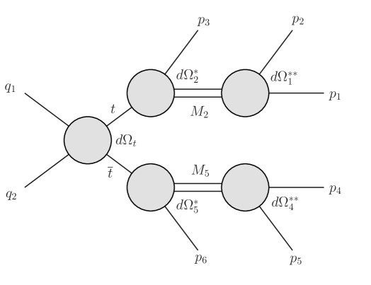
Figure 1: Kinematics for $gg\to t{\overline{t}}\to\left(b{\overline{b}}c\right)\left({\overline{b}}\ell{\overline{\nu}}\right)$ ggprocesskinematics . The definitions of the various angles and invariant masses are identical to those given in Ref. tNPLHC1 ; these definitions are reproduced here for convenience. $\Omega_{1}^{**}$ denotes the direction of $\vec{p}_{1}^{~{}**}$ in the rest frame of $M_{2}$, relative to the direction of $\vec{p}_{1}^{~{}*}+\vec{p}_{2}^{~{}*}$, where $M_{2}^{2}=(p_{1}+p_{2})^{2}$. Similarly, $\Omega_{2}^{*}$ denotes the direction of $\left(\vec{p}_{1}^{~{}*}+\vec{p}_{2}^{~{}*}\right)$ in the $t$ rest frame, relative to the direction of $\vec{p}_{t}$ in the $t{\overline{t}}$ rest frame. $\Omega_{t}$ denotes the direction of $\vec{p}_{t}$ relative to $\vec{q}_{1}$, also in the $t{\overline{t}}$ rest frame. The solid angles $\Omega_{4}^{**}$ and $\Omega_{5}^{*}$ are defined analogously to $\Omega_{1}^{**}$ and $\Omega_{2}^{*}$, respectively, and $M_{5}^{2}=(p_{4}+p_{5})^{2}$. In this work we take $p_{1}=p_{c}$, $p_{2}=p_{b}$, $p_{3}=p_{\overline{b}_{1}}$, $p_{4}=p_{\overline{\nu}}$, $p_{5}=p_{\overline{b}_{2}}$ and $p_{6}=p_{\ell}$.

The kinematics of the process $gg\to t{\overline{t}}\to\left(b{\overline{b}}c\right)\left({\overline{b}}\ell{\overline{\nu}}\right)$ is represented in Fig. 1. As described in Ref. tNPLHC1 , the six-body phase space may be decomposed into five solid angles and four invariant masses. Note that Fig. 1 represents only the kinematics of $gg\to t{\overline{t}}\to\left(b{\overline{b}}c\right)\left({\overline{b}}\ell{\overline{\nu}}\right)$ – it is not a Feynman diagram. Thus, $M_{5}^{2}$ does not necessarily correspond to the $W^{-}$ resonance in the ${\overline{t}}$ decay, and $M_{2}^{2}$ does not necessarily correspond to the $W^{+}$ resonance in the SM part of the $t$ decay. Rather, $p_{1}$, $p_{2}$ and $p_{3}$ are the momenta of the $b$, ${\overline{b}}$ and $c$ quarks in $t\to b{\overline{b}}c$, with all permutations being allowed. Assuming that the $t$ and ${\overline{t}}$ quarks are on-shell before decaying, two of the invariant-mass degrees of freedom can be eliminated. The solid angles $d\Omega_{1}^{**}$, $d\Omega_{2}^{*}$, $d\Omega_{4}^{**}$, $d\Omega_{5}^{*}$ and $d\Omega_{t}$ in Fig. 1 are defined in five different rest frames, with the $*$ and $**$ superscripts indicating that these angles are defined in reference frames that are, respectively, one and two boosts away from the $t{\overline{t}}$ rest frame. The invariant masses $M_{2}$ and $M_{5}$ are defined via $M_{2}^{2}=\left(p_{1}+p_{2}\right)^{2}$ and $M_{5}^{2}=\left(p_{4}+p_{5}\right)^{2}$. The differential cross section is a complicated function of the various momenta [see Eqs. (A.1)-(A.4)]; these momenta may in turn be related back to the solid angles and invariant masses via boosts and rotations.

The approximate analytical expression for the differential cross section for $gg\to t{\overline{t}}\to(b{\overline{b}}c)({\overline{b}}\ell{\overline{\nu}})$ was derived making several simplifying assumptions:

1. We considered only the $gg$ initial state, ignoring $q\overline{q}$ initial states.

2. We ignored the parton distribution functions (PDFs) for the initial gluons and worked in the rest frame of the initial $gg$ pair. In the actual experiment, the initial gluons have a wide range of momenta, and the lab frame is generally different than the $gg$ rest frame for a given event.

3. We considered the final state $\overline{b}$’s to be “distinguishable,” when in fact they are identical particles.

In addition to the above simplifications, we also set the masses of the light quarks and the charged lepton to zero. The analytical expressions for the differential cross section and integrated cross section for $gg\to t{\overline{t}}\to\left(b{\overline{b}}c\right)\left({\overline{b}}\ell{\overline{\nu}}\right)$ are given in Appendix A. At first glance, it might appear that the above assumptions would have rendered these expressions almost completely useless. On the contrary, however, we have found that these expressions provide crucial insights into the actual physical process and serve as a useful starting point for a more robust numerical treatment of the problem.

In Refs. tNPLHC1 ; tNPLHC2 we focused primarily on CP-even observables. In the present work we turn our attention to CP-odd observables. We proceed in the same manner as we did in Refs. tNPLHC1 ; tNPLHC2 , working first from theoretical expressions derived under various simplifying assumptions, and turning later to a more robust numerical treatment.

III CP-violating Observables in $gg\to t{\overline{t}}\to\left(b{\overline{b}}c\right)\left({\overline{b}}\ell{\overline{\nu}}\right)$

A perusal of the general expressions for the differential and integrated cross sections for $gg\to t(\to b{\overline{b}}c){\overline{t}}(\to{\overline{b}}\ell{\overline{\nu}})$ shows that that there are two CP-odd combinations of NP parameters that can be probed in this process, namely Im($X^{V*}_{LL}$) [Eq. (A.13)] and Im($X^{T}_{LL}X^{S*}_{LL}+X^{T}_{RR}X^{S*}_{RR}$) [Eq. (A.3)]. These same two parameter combinations were analyzed in Ref. kklrsw , although the notation in that paper was somewhat different. In addition, for Im($X^{T}_{LL}X^{S*}_{LL}+X^{T}_{RR}X^{S*}_{RR}$) it was assumed there that the spin of the top quark could be measured (obviously a simplifying assumption). In the present context, the correlations between the pair-produced $t$ and ${\overline{t}}$ effectively allow us to gain access to the spin of the top.

The CP-violating observables that will allow experimentalists to measure the above CP-odd NP parameter combinations are as follows. Im($X^{V*}_{LL}$) is probed using the partial-rate asymmetry, while Im($X^{T}_{LL}X^{S*}_{LL}+X^{T}_{RR}X^{S*}_{RR}$) appears in triple products and can be probed in several ways. In the following subsections we describe each of these observables in turn. Note that the analytic expressions, wherever quoted, have been derived with the simplifying assumptions discussed above.

III.1 Partial rate asymmetry

The simplest CP-odd observable may be obtained by comparing the cross section for the process $gg\to t{\overline{t}}\to\left(b{\overline{b}}c\right)\left({\overline{b}}\ell{\overline{\nu}}\right)$ to that for the conjugate process $gg\to t{\overline{t}}\to\left(b\bar{\ell}\nu\right)\left(b{\overline{b}}\bar{c}\right)$. Now, CP-violating effects can only arise as a result of the interference of two amplitudes. Furthermore, all signals of direct CP violation, such as the partial-rate asymmetry (PRA), are proportional to the CP-odd quantity $\sin\phi\sin\delta$, where $\phi$ and $\delta$ are respectively the weak-phase and strong-phase differences between the two amplitudes. As noted in Sec. II.1, the NP strong phases are negligible, so $\delta$ is due entirely to the SM $W$-mediated amplitude. Furthermore, the weak phase must arise entirely from NP since the SM weak phase is $\simeq 0$. Therefore, the PRA is due to SM-NP interference. The only NP contribution that interferes with the SM is the $(V-A)\times(V-A)$ term in the effective Lagrangian. As a result, the PRA is proportional to the width of the $W$ and to Im($X^{V*}_{LL}$).

Normalizing to the sum of the cross sections, the PRA can be written

$${\cal A}=\frac{\sigma-\overline{\sigma}}{\sigma+\overline{\sigma}}\simeq\frac{1}{\cal R}\frac{4\Gamma_{W}}{m_{W}}\mbox{Im}\left(X^{V*}_{LL}\right),$$ (4)

where

$${\cal R}=\frac{\sigma+\overline{\sigma}}{2\sigma_{\mbox{\scriptsize SM}}}=1+\frac{3G_{F}m_{t}^{2}}{4\sqrt{2}\pi^{2}\left(1-\zeta_{W}^{2}\right)^{2}\left(1+2\zeta_{W}^{2}\right)}\sum_{i,\sigma}\hat{A}_{i}^{\sigma}$$ (5)

with $\zeta_{W}\equiv m_{W}/m_{t}$ and $\hat{A}_{i}^{\sigma}$ being combinations of various $X^{I}_{AB}$, as defined in Eq. (A.10).

While the presence of the ratio $\Gamma_{W}/m_{W}$ in Eq. (4) leads to a suppression of the PRA, it is still possible to obtain an asymmetry whose magnitude is in excess of 10% kklrsw . And, despite this suppression, the PRA still offers several advantages. The foremost among these is that it is relatively straightforward to measure, since it does not require a detailed kinematical analysis or the determination of angles in various rest frames. One simply counts the number of events for the $t$ decay in this channel and compares that to the number of events for the ${\overline{t}}$ decay in the analogous channel. In fact, since the PRA does not require the presence of correlations between the pair-produced $t$ and ${\overline{t}}$, we needn’t be so restrictive regarding the decay mode of the “other” particle. That is, we could just as well compare the width for $gg\to t(\to b{\overline{b}}c){\overline{t}}(\to\mbox{everything})$ to that for $gg\to{\overline{t}}(\to{\overline{b}}b{\overline{c}})t(\to\mbox{everything})$ in order to increase statistics (assuming, of course, that the process and conjugate process could still be distinguished without tagging on the charge of the lepton). We present the numerical results for benchmark NP scenarios in Sec. IV.1.

III.2 Triple product

In decay processes with two contributing amplitudes $A$ and $B$, the square of the total amplitude may contain interference terms of the form Im($AB^{*}$)[$\vec{v}_{1}\cdot(\vec{v}_{2}\times\vec{v}_{3})$], where each $v_{i}$ is a spin or a momentum. These triple products (TPs) are odd under time reversal (T) and hence, by the CPT theorem, also constitute potential signals of CP violation. Now,

$${\rm Im}(AB^{*})=|A||B|(\sin\phi\cos\delta+\cos\phi\sin\delta)~{},$$ (6)

where $\phi$ and $\delta$ are respectively the weak-phase and strong-phase differences between $A$ and $B$. The first term is CP-odd, while the second is CP-even, so that the TP is not by itself a signal of CP violation (this is due to the fact that T is an anti-unitary operator). On the other hand, the TP in the CP-conjugate process is proportional to

$${\rm Im}(AB^{*})_{CP-conj}=|A||B|(-\sin\phi\cos\delta+\cos\phi\sin\delta)~{}.$$ (7)

Combining ${\rm Im}(AB^{*})$ and ${\rm Im}(AB^{*})_{CP-conj}$ allows one to isolate the CP-odd piece proportional to $\sin\phi\cos\delta$. That is, as with direct CP violation (the PRA), in order to obtain a CP-violating signal, one must compare the TP in the process with that in the CP-conjugate process. However, in contrast to direct CP violation, no strong-phase difference between the interfering amplitudes is required in order to obtain a non-vanishing CP-violating signal (i.e. $\delta$ can be 0). It is interesting to note that, if the strong phase difference is indeed negligible ($\delta\approx 0$), then the CP-even term (proportional to $\cos\phi\sin\delta$) is approximately zero, which then makes the TP a signal of CP-violation by itself.

In Ref. kklrsw , it was shown that, in the presence of NP, a TP of the form $\vec{s}_{t}\cdot\left(\vec{p}_{\overline{b}}\times\vec{p}_{c}\right)$ can be generated in the decay $t\to b{\overline{b}}c$. Here $\vec{s}_{t}$ denotes the spin of the $t$, and $\vec{p}_{i}$ is the momentum of the particle $i$ coming from the decay of the $t$. Since the top decays, one might try to gain access to the top’s spin via correlations with the momenta of its decay products. Such an approach cannot give access to a quantity such as $\vec{s}_{t}\cdot\left(\vec{p}_{\overline{b}}\times\vec{p}_{c}\right)$, however, since the three momenta $\vec{p}_{i}$ ($i=b,{\bar{b}},c$) are not independent. The problem can be circumvented by using the fact that, in $t{\overline{t}}$ production, the spins of the $t$ and the ${\overline{t}}$ are statistically correlated spincorrexpt . As $\vec{s}_{\overline{t}}$ is related to the momenta of the decay products of the ${\overline{t}}$, the TP in $t\to b{\overline{b}}c$ can be rewritten as a TP involving three final-state momenta of the full process, $gg\to t(\to b{\overline{b}}c){\overline{t}}(\to{\overline{b}}\ell{\overline{\nu}})$, and this does not vanish. In practice, this is implemented by introducing the $t{\overline{t}}$ spin-correlation coefficient:

$$\kappa_{t{\overline{t}}}\quad=\quad\dfrac{\sigma_{\uparrow\uparrow}+\sigma_{\downarrow\downarrow}-\sigma_{\uparrow\downarrow}-\sigma_{\downarrow\uparrow}}{\sigma_{\uparrow\uparrow}+\sigma_{\downarrow\downarrow}+\sigma_{\uparrow\downarrow}+\sigma_{\downarrow\uparrow}}~{}.$$ (8)

Here, $\uparrow$ and $\downarrow$ denote the alignment of the spins of the top and antitop with respect to the chosen spin-quantization axis. As noted above, $\vec{s}_{t}$ is related to the momenta, or angular distribution, of the $t$ decay products, and similarly for $\vec{s}_{\overline{t}}$. The TP in $gg\to t(\to b{\overline{b}}c){\overline{t}}(\to{\overline{b}}\ell{\overline{\nu}})$ then involves the angular correlation between the decay products of the two particles. As is evident in Eq. (A.3), there are also triple-product terms relating the initial-state gluons and the decay products of the top.

As was noted above, the CP-odd combination of NP parameters that shows up in the triple-product terms is Im($X^{T}_{LL}X^{S*}_{LL}+X^{T}_{RR}X^{S*}_{RR}$) (see Appendix 1). That is, the TP is due to NP-NP interference. Furthermore, since the NP strong phases are negligible, $\delta=0$ in Eqs. (6) and (7). Hence, following the discussion below Eq. (7), the TP by itself is a signal of CP-violation in $gg\to t{\overline{t}}\to\left(b{\overline{b}}c\right)\left({\overline{b}}\ell{\overline{\nu}}\right)$. In the sub-sections that follow we identify observables that can be used to isolate the TP and quantify the resulting CP-violation.

III.2.1 Angular Distributions

The first observable is the double differential distribution relative to the angles $\theta_{5}^{*}$ and $\phi_{1}^{**}$. Of these, $\theta_{5}^{*}$ is related to the lepton polar angle in the $\overline{t}$ rest frame, while $\phi_{1}^{**}$ is an azimuthal angle in the $b$-$c$ rest frame. Integrating the differential cross section over all phase-space variables except for these two angles yields

$$\frac{d\sigma}{d\!\cos\theta_{5}^{*}\,d\phi_{1}^{**}} = \frac{\sigma_{\mbox{\scriptsize SM}}}{4\pi}\Bigg{\{}1+\frac{4\Gamma_{W}}{m_{W}}\mbox{Im}\left(X^{V*}_{LL}\right)\;+\;\frac{3G_{F}m_{t}^{2}}{4\sqrt{2}\pi^{2}\left(1-\zeta_{W}^{2}\right)^{2}\left(1+2\zeta_{W}^{2}\right)}\Bigg{(}\sum_{i,\sigma}\hat{A}{{}_{i}^{\sigma}}$$ (9)

$$\mspace{60.0mu}+\;\frac{2\pi^{2}\kappa(r)}{35}\Big{[}\cos\theta_{5}^{*}\cos\phi_{1}^{**}\left(\hat{A}_{b}^{-}-\hat{A}_{b}^{+}-\hat{A}_{c}^{-}+\hat{A}_{c}^{+}\right)$$

$$\mspace{115.0mu}+\;16\cos\theta_{5}^{*}\sin\phi_{1}^{**}\mbox{Im}\!\left[X^{T}_{LL}X^{S*}_{LL}+X^{T}_{RR}X^{S*}_{RR}\right]\Big{]}\Bigg{)}\Bigg{\}},$$

where $\sigma_{\rm SM}$ is given by Eq. (A.11), $\zeta_{W}=m_{W}/m_{t}$ and

$$\kappa(r) =\;\;\frac{\left(-31r^{4}+37r^{2}-66\right)r-2\left(r^{6}-17r^{4}+33r^{2}-33\right)\tanh^{-1}\left(r\right)}{r^{2}\left[\left(31r^{2}-59\right)r+2\left(r^{4}-18r^{2}+33\right)\tanh^{-1}\left(r\right)\right]}~{},$$ (10)

with $r=\sqrt{1-4m_{t}^{2}/Q^{2}}$ and $Q\equiv p_{t}+p_{\overline{t}}$. Note that $\kappa(r)$, as defined above, differs from $\kappa_{t\overline{t}}$ in Eq. (8) by an overall sign; also, $\kappa_{t\overline{t}}$ is averaged over energies.

Equation (9) contains both CP-even and CP-odd terms. The part of the expression that is proportional to $\kappa(r)$ arises from $t{\overline{t}}$ spin correlations Soni . These terms disappear upon integration over the angles $\theta_{5}^{*}$ and $\phi_{1}^{**}$, as one might expect.

The term proportional to $\cos\theta_{5}^{*}\cos\phi_{1}^{**}$ in Eq. (9) is sensitive to the CP-even combination of NP parameters $(\hat{A}_{b}^{-}-\hat{A}_{b}^{+}-\hat{A}_{c}^{-}+\hat{A}_{c}^{+})$. This combination is distinct from the NP parameter combinations that arise in the observables described in Refs. tNPLHC1 and tNPLHC2 . Thus, although our emphasis in the present work is on CP-odd observables, we note that Eq. (9) leads to a complementary approach to measuring CP-even combinations of NP parameters. The term that is of primary interest to us in this work is the one proportional to $\cos\theta_{5}^{*}\sin\phi_{1}^{**}$. This term arises from the triple-product terms in $t\to b{\overline{b}}c$ and contains the CP-odd NP parameter combination Im($X^{T}_{LL}X^{S*}_{LL}+X^{T}_{RR}X^{S*}_{RR}$). The value of Im($X^{T}_{LL}X^{S*}_{LL}+X^{T}_{RR}X^{S*}_{RR}$) can be extracted directly by fitting the angular distribution in Eq. (9) using the template method developed in Ref. tNPLHC2 . We perform such a fit here for a few benchmark NP scenarios. The details of the fitting procedure, our choice of templates, as well as the results are presented in Sec.IV.2.1.

III.2.2 $\langle\cos\theta_{5}^{*}\sin\phi_{1}^{**}\rangle$

Equation (9) is also suggestive of a second observable that can be used to extract the value of Im($X^{T}_{LL}X^{S*}_{LL}+X^{T}_{RR}X^{S*}_{RR}$). This is the expectation value of $\cos\theta_{5}^{*}\sin\phi_{1}^{**}$. Taking into account the overall normalization, we find

$$\langle\cos\theta_{5}^{*}\sin\phi_{1}^{**}\rangle\;=\;\frac{\sigma_{\mbox{\scriptsize SM}}}{\sigma}\left(\frac{2\sqrt{2}G_{F}m_{t}^{2}\kappa(r)}{35\left(1-\zeta_{W}^{2}\right)^{2}\left(1+2\zeta_{W}^{2}\right)}\right)\mbox{Im}\!\left[X^{T}_{LL}X^{S*}_{LL}+X^{T}_{RR}X^{S*}_{RR}\right]\mspace{20.0mu}$$ (11)

for a fixed value of the gluon energy. For $pp$ collisions, one convolutes over parton distribution functions. This can be incorporated in an approximate way by making the replacement $\kappa(r)\to\langle\kappa(r)\rangle$, with $\langle\kappa(r)\rangle$ being measured over the events included in the analysis. From Eq. (11) we see that $\langle\cos\theta_{5}^{*}\sin\phi_{1}^{**}\rangle\left(\sigma/\sigma_{\mbox{\scriptsize SM}}\right)$ as a function of $\mbox{Im}\!\left[X^{T}_{LL}X^{S*}_{LL}+X^{T}_{RR}X^{S*}_{RR}\right]$ is expected to be a straight line passing through the origin. However, as mentioned earlier, this expression has been derived under the simplifying assumptions discussed in Sec.II.2. To see how well this relation holds up in a more realistic scenario, we perform a Monte Carlo simulation where we generate data sets with different choices for $\mbox{Im}\!\left[X^{T}_{LL}X^{S*}_{LL}+X^{T}_{RR}X^{S*}_{RR}\right]$. The results are detailed in Sec.IV.2.2.

III.2.3 $A_{\rm TP}$

The third observable that can be used to capture the effect of the TP is the quantity $A_{\rm TP}$, which we define as

$$A_{\rm TP}\quad=\quad\dfrac{N[\epsilon(p_{b},p_{\bar{b}},p_{c},p_{\ell})>0]\;\;-\;\;N[\epsilon(p_{b},p_{\bar{b}},p_{c},p_{\ell})<0]}{N[\epsilon(p_{b},p_{\bar{b}},p_{c},p_{\ell})>0]\;\;+\;\;N[\epsilon(p_{b},p_{\bar{b}},p_{c},p_{\ell})<0]}\,,$$ (12)

where $\epsilon(p_{b},p_{\bar{b}},p_{c},p_{\ell})=\epsilon_{\mu\nu\rho\lambda}\,p_{b}^{\mu}\,p_{\bar{b}}^{\nu}\,p_{c}^{\rho}\,p_{\ell}^{\lambda}$ with $\epsilon^{0123}=+1$.

Equation (A.3) contains several terms of the type $\epsilon(q_{i},q_{j},q_{k},q_{l})$, where the $q_{i}$ are momenta or combinations of momenta of the initial and/or final state particles. Of these, one expects that $\epsilon(p_{b},p_{\bar{b}},p_{c},p_{\ell})$ would be quite amenable to experimental measurement, as it only involves the measurement of the 4-momenta of the final state $b$, $\bar{b}$, $c$ and lepton. Moreover, it does not require the reconstruction of any special frames of reference and can be measured in the lab frame itself. Note that the measurement of $A_{\rm TP}$ would not lead to the measurement of Im($X^{T}_{LL}X^{S*}_{LL}+X^{T}_{RR}X^{S*}_{RR}$) as such. Nevertheless, a non-zero value of $A_{\rm TP}$ would be a smoking gun signal of the presence of CP-violating NP. Furthermore, upon measurement of a non-zero signal, it is expected that detailed numerical simulations could be used to constrain the value of Im($X^{T}_{LL}X^{S*}_{LL}+X^{T}_{RR}X^{S*}_{RR}$).

Once again, we perform a Monte Carlo simulation for certain benchmark NP scenarios, the results of which are presented in Sec. IV.2.3.

IV Numerical Results

In this section we present the results of the numerical simulations to which we have alluded earlier. All the analytic expressions presented hitherto were obtained under the simplifying assumptions discussed in Sec.II.2. However, for our numerical analysis we return to a more realistic treatment. To be specific :

1. We include the contribution from $q\overline{q}$ initial states. This can be calculated in a manner similar to that used for obtaining the $gg$ contribution (see Appendix B). At the LHC, it gives only a sub-dominant contribution ($\sim$ 10%-15%). Nevertheless, it is interesting to note that the structure of distributions such as the one in Eq. (9) remains the same. In fact, the only change appears in the expressions for $\sigma_{\rm SM}$ and $\kappa(r)$. This, of course, is expected because in Eq. (9), these are the only two pieces that depend on the $t\bar{t}$ production mechanism. The rest relates exclusively to the dynamics of the decay.

2. We incorporate PDFs appropriately for the initial state partons.

3. We implement a procedure to distinguish between the identical $\bar{b}$’s in the final state and identify “correctly” the $\bar{b}$ coming from the $t$ decay. To do this, we construct the quantities $m_{1}^{2}=(p_{b}+p_{c}+p_{\bar{b}_{1}})^{2}$ and $m_{2}^{2}=(p_{b}+p_{c}+p_{\bar{b}_{2}})^{2}$. If both $m_{1}$ and $m_{2}$ lie within $m_{t}\pm 15\Gamma_{t}$, the event is discarded. Otherwise, the $\bar{b}_{i}$ that leads to a smaller value of $|m_{i}-m_{t}|$ is assumed to come from the $t$ decay. For the conjugate process ($pp\to t(\to b\bar{\ell}\nu){\overline{t}}(\to{\overline{b}}b{\overline{c}}))$, a similar criterion is applied to the $b$’s. The result is a loss of $\sim$ 20% of the events for both process and conjugate process.

In addition, in generating the simulation data, we allow the light quarks and the charged lepton to have non-zero masses. The event samples have been generated using MadGraph5 MG5 in conjuction with FeynRules FR . We consider a few benchmark NP scenarios to test the efficacy of the observables discussed above. $\sqrt{s}$ is taken to be 14 TeV and CTEQ6L CTEQ parton distribution functions are used with both factorization and renormalization scales set to $m_{t}$ = 172 GeV. The integrated luminosity corresponds to $10^{5}$ SM events of the type $pp\to t{\overline{t}}\to\left(b{\overline{b}}c\right)\left({\overline{b}}\ell{\overline{\nu}}\right)$, which is expected to be achieved by the year 2030 SteveMyers .

IV.1 Partial rate asymmetry - Results

In this section we consider two benchmark NP scenarios, which we label EX-A and EX-B. It is clear from Table 1 that even when Im($X^{V*}_{LL}$) $\sim{\cal O}$(1), ${\cal A}$ can be fairly large ($\sim$ 10%). We also use Eqs. (4) and (5) to extract the value of Im($X^{V*}_{LL}$) from the “data”. Note that in real life we would have no a priori knowledge of the $\hat{A}^{\sigma}_{i}$’s. Therefore ${\cal R}$ would have to be calculated in terms of the observed $\sigma$ and $\bar{\sigma}$ and the expected $\sigma_{\rm SM}$. As can be seen from the last column of Table 1, the values of Im($X^{V*}_{LL}$) are recovered quite accurately. As expected, the PRA provides a simple and effective way to capture the effect of CP-violation in $t\to b{\overline{b}}c$.

Model	Input Im($X^{V*}_{LL}$)	${\cal A}=\dfrac{N-\overline{N}}{N+\overline{N}}$	Extracted value of Im($X^{V*}_{LL}$)
SM	0.0	$-$0.002 $\pm$ 0.002	$-$0.01 $\pm$ 0.02
EX-A	$-$3.0	$-$0.117 $\pm$ 0.001	$-$2.97 $\pm$ 0.03
EX-B	$-$2.0	$-$0.060 $\pm$ 0.001	$-$1.97 $\pm$ 0.04

Table 1: Partial rate asymmetries and recovered NP parameter values for the SM and two NP models.

IV.2 Triple product - Results

IV.2.1 Angular Distributions

In an experiment, a distribution of the type of Eq. (9) would be measured as a 2-D histogram, D. We see that the RHS of Eq. (9) can be expressed as the sum of five terms – one term independent of NP parameters and four terms dependent on Im($X^{V*}_{LL}$), $\sum\hat{A}_{i}^{\sigma}$, $(\hat{A}_{b}^{-}-\hat{A}_{b}^{+}-\hat{A}_{c}^{-}+\hat{A}_{c}^{+})$ and Im($X^{T}_{LL}X^{S*}_{LL}+X^{T}_{RR}X^{S*}_{RR}$), respectively. Using MadGraph5, and with appropriate choices for the $X^{I}_{AB}$, one can generate this angular distribution for a case where only one of the NP parameter combinations is non-zero and all others are zero. This can be done in turn for each of the four combinations. In addition, there would be the case corresponding to the SM, where all the NP parameter-combinations are zero. These histograms form the templates that we label TM-0, TM-1, TM-2, TM-3, TM-4. Now the measured histogram D, in which the NP parameters take arbitrary, unknown values, can be expressed as a linear combination of the templates TM-i with appropriate weights; i.e.,

$$\mathtt{D\quad=\quad w_{0}\texttt{TM-{0}}\;+\;w_{1}\texttt{TM-{1}}\;+\;w_{2}\texttt{TM-{2}}\;+\;w_{3}\texttt{TM-{3}}\;+\;w_{4}\texttt{TM-{4}}\,.}$$ (13)

The weights $\mathtt{w_{i}}$ can be determined through a simple fitting procedure such as $\chi^{2}$ minimization and be used to extract the values of Im($X^{V*}_{LL}$), $\sum\hat{A}_{i}^{\sigma}$, $(\hat{A}_{b}^{-}-\hat{A}_{b}^{+}-\hat{A}_{c}^{-}+\hat{A}_{c}^{+})$ and Im($X^{T}_{LL}X^{S*}_{LL}+X^{T}_{RR}X^{S*}_{RR}$) encoded in the data histogram D.

While the idea is simple, there are a few subtleties that must be taken care of during its implementation:

• First, the parameter inputs are provided in terms of $X^{I}_{AB}$. By doing so it is possible to ensure that only one $\hat{A}^{\sigma}_{i}$ is non-zero at a time. However, it can still lead to overlapping contributions in the templates that we are interested in. For example, a non-zero input for $\hat{A}^{+}_{c}$ makes $\sum\hat{A}_{i}^{\sigma}$ as well as $(\hat{A}_{b}^{-}-\hat{A}_{b}^{+}-\hat{A}_{c}^{-}+\hat{A}_{c}^{+})$ non-zero simultaneously. These kinds of overlaps need to be removed. How we do this can be seen in Table 2.

• Second, a $\chi^{2}$ fit, by construction, can only distinguish between terms with different angular structure. Equation (9) contains three terms with no angular dependence: the SM term, the term proportional to Im($X^{V*}_{LL}$) and the term proportional to $\sum\hat{A}_{i}^{\sigma}$. The fit is not capable of identifying the contributions coming from these three pieces separately. To circumvent this problem, we fix the SM contribution to 1.0 and assume that Im($X^{V*}_{LL}$) could be fixed to the value obtained by measuring the PRA. Thereafter we extract the values of $\sum\hat{A}_{i}^{\sigma}$, $(\hat{A}_{b}^{-}-\hat{A}_{b}^{+}-\hat{A}_{c}^{-}+\hat{A}_{c}^{+})$ and Im($X^{T}_{LL}X^{S*}_{LL}+X^{T}_{RR}X^{S*}_{RR}$).

• Third, the template distributions must be subjected to the same selection criteria, cuts, etc. as the data.

We implement this fitting algorithm for two NP scenarios. Once again, we generate “pseudo-data” using MadGraph5. Here we have specifically chosen NP scenarios where Im($X^{V*}_{LL}$) = 0, to demonstrate the efficacy of the procedure in the “best-case” scenario when Im($X^{V*}_{LL}$) is actually 0. In the case of non-zero Im($X^{V*}_{LL}$), the value of Im($X^{V*}_{LL}$) estimated from the PRA is an input to the fit. This is also true of the observables discussed in Refs. tNPLHC1 and tNPLHC2 where we focused primarily on CP-even observables and set Im($X^{V*}_{LL}$) to zero in much of the analysis. Hence, while attempting to extract NP parameters in $t\to b{\overline{b}}c$, the first task would be to measure the PRA and the value of Im($X^{V*}_{LL}$).

The results of the fit are presented in Table 3. It can be seen that, despite all the complications, the extracted values lie relatively close to the input values, although some of the fit values are several standard deviations away from the corresponding inputs. More importantly, the presence of NP, of both CP-conserving and CP-violating varieties, is firmly established.

Template	$X^{I}_{AB}$	$\hat{A}_{i}^{\sigma}$	Surviving Contribution
TM-0	All $X^{I}_{AB}$ = 0	All $\hat{A}_{i}^{\sigma}$ = 0	SM
TM-1	TME-5 $-$ TME-1		Im($X^{V*}_{LL}$)
TM-2	TME-2 $+$ TME-3		$\sum\hat{A}^{\sigma}_{i}$
TM-3	TME-2 $-$ TME-3		$(\hat{A}_{b}^{-}-\hat{A}_{b}^{+}-\hat{A}_{c}^{-}+\hat{A}_{c}^{+})$
TM-4	TME-4 $-$ TME-1 $-$ TME-2		Im($X^{T}_{LL}X^{S*}_{LL}+X^{T}_{RR}X^{S*}_{RR}$)
TME-1	Re($X^{V}_{LL}$) $\neq$ 0	$\hat{A}_{{\overline{b}}}^{+}$ $\neq$ 0; all other $\hat{A}_{i}^{\sigma}$ = 0	$\hat{A}_{{\overline{b}}}^{+}$
TME-2	$X^{V}_{LR}$ $\neq$ 0	$\hat{A}_{c}^{+}$ $\neq$ 0; all other $\hat{A}_{i}^{\sigma}$ = 0	$\hat{A}_{c}^{+}$
TME-3	$X^{V}_{RL}$ $\neq$ 0	$\hat{A}_{c}^{-}$ $\neq$ 0; all other $\hat{A}_{i}^{\sigma}$ = 0	$\hat{A}_{c}^{-}$
TME-4	Re($X^{S}_{LL}$) $\neq$ 0 ;	$\hat{A}_{{\overline{b}}}^{+}$, $\hat{A}_{c}^{+}$ $\neq$ 0 ;	$\hat{A}_{{\overline{b}}}^{+}$, $\hat{A}_{c}^{+}$,
	Im($X^{T}_{LL}$) $\neq$ 0	all other $\hat{A}_{i}^{\sigma}$ = 0	Im($X^{T}_{LL}X^{S*}_{LL}+X^{T}_{RR}X^{S*}_{RR}$)
TME-5	Im($X^{V}_{LL}$) $\neq$ 0	$\hat{A}_{{\overline{b}}}^{+}$ $\neq$ 0; all other $\hat{A}_{i}^{\sigma}$ = 0	$\hat{A}_{{\overline{b}}}^{+}$, Im($X^{V*}_{LL}$)

Table 2: NP parameter choices for each of the templates. TM-0, TM-1, TM-2, TM-3, TM-4 are the ones actually included in the fit. The template histograms have been generated with $10^{6}$ events each so that the statistical uncertainty originating from them is negligible and does not affect the fit.

Model	Parameter	Input Value	Fit Result	$\chi^{2}$/d.o.f.
EX-C	$\hat{A}_{c}^{+}+\hat{A}_{c}^{-}+\hat{A}_{\bar{b}}^{+}+\hat{A}_{\bar{b}}^{-}+\hat{A}_{b}^{+}+\hat{A}_{b}^{-}$	64	65.7 $\pm$ 0.3	1.2
	$\hat{A}_{b}^{-}-\hat{A}_{b}^{+}-\hat{A}_{c}^{-}+\hat{A}_{c}^{+}$	32	29.5 $\pm$ 4.1
	Im($X^{T}_{LL}X^{S*}_{LL}+X^{T}_{RR}X^{S*}_{RR}$)	4	3.1 $\pm$ 0.2
EX-D	$\hat{A}_{c}^{+}+\hat{A}_{c}^{-}+\hat{A}_{\bar{b}}^{+}+\hat{A}_{\bar{b}}^{-}+\hat{A}_{b}^{+}+\hat{A}_{b}^{-}$	77	77.6 $\pm$ 0.3	1.3
	$\hat{A}_{b}^{-}-\hat{A}_{b}^{+}-\hat{A}_{c}^{-}+\hat{A}_{c}^{+}$	67	62.8 $\pm$ 4.4
	Im($X^{T}_{LL}X^{S*}_{LL}+X^{T}_{RR}X^{S*}_{RR}$)	3.5	2.8 $\pm$ 0.2

Table 3: Input values and fit results for the double differential distribution in $\cos(\theta_{5}^{*})$ and $\phi_{1}^{**}$. The theoretical expression for the angular distribution is given in Eq. (9); the actual fit is performed using templates, as described by Eq. (13).

IV.2.2 $\langle\cos\theta_{5}^{*}\sin\phi_{1}^{**}\rangle$

In Sec. III.2.2, we saw that $\langle\cos\theta_{5}^{*}\sin\phi_{1}^{**}\rangle$ can be expressed as

$$\langle\cos\theta_{5}^{*}\sin\phi_{1}^{**}\rangle\quad =\quad\frac{\sigma_{\mbox{\scriptsize SM}}}{\sigma}\;\;{\cal W}\;\;\mbox{Im}\!\left[X^{T}_{LL}X^{S*}_{LL}+X^{T}_{RR}X^{S*}_{RR}\right]\mspace{150.0mu}$$

$$\text{where}\mspace{90.0mu}{\cal W}\quad =\quad\left(\frac{2\sqrt{2}G_{F}m_{t}^{2}\;\langle\kappa(r)\rangle}{35\left(1-\zeta_{W}^{2}\right)^{2}\left(1+2\zeta_{W}^{2}\right)}\right)\,.$$

Using MadGraph5, we generate several data-sets with different input values of Im[$X^{T}_{LL}X^{S*}_{LL}+X^{T}_{RR}X^{S*}_{RR}$]. We then calculate and plot $(\sigma/\sigma_{\rm SM})\,(\langle\cos\theta_{5}^{*}\sin\phi_{1}^{**}\rangle)$ for each data-set. These are shown as orange ‘$+$’s in Fig. 2. We also calculate and plot ${\cal W}$ Im[$X^{T}_{LL}X^{S*}_{LL}+X^{T}_{RR}X^{S*}_{RR}$] using the input value of Im[$X^{T}_{LL}X^{S*}_{LL}+X^{T}_{RR}X^{S*}_{RR}$] and the value of $\langle\kappa(r)\rangle$ obtained from the SM data-set. These are the blue $\times$s in Fig. 2. We see that, although the ‘$+$’s and ‘$\times$’s do not coincide, $(\sigma/\sigma_{\rm SM})\,(\langle\cos\theta_{5}^{*}\sin\phi_{1}^{**}\rangle)$ is, nonetheless, a linear function of Im[$X^{T}_{LL}X^{S*}_{LL}+X^{T}_{RR}X^{S*}_{RR}$] with zero intercept.

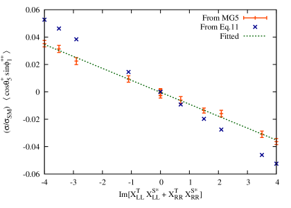
Figure 2: Plot of $(\sigma/\sigma_{\rm SM})\,(\langle\cos\theta_{5}^{*}\sin\phi_{1}^{**}\rangle)$ as a function of Im[$X^{T}_{LL}X^{S*}_{LL}+X^{T}_{RR}X^{S*}_{RR}$] for various combinations of NP parameters. As is evident from the plot, the simulated data has a linear dependence on Im[$X^{T}_{LL}X^{S*}_{LL}+X^{T}_{RR}X^{S*}_{RR}$], as in Eq. (11), even though Eq. (11) was derived under several simplifying assumptions.

The linearity of the plot in Fig. 2 has important ramifications. Firstly, we realize that a measurement of $\langle\cos\theta_{5}^{*}\sin\phi_{1}^{**}\rangle$ is, by itself, sufficient to indicate the presence of CP-violating new physics in $t\to b{\overline{b}}c$. Secondly, if such new physics does indeed exist in nature, then knowledge of the slope of the green dashed line in Fig. 2, along with $\sigma_{\mbox{\scriptsize SM}}$, puts us in a position to directly extract the value of $\mbox{Im}\!\left[X^{T}_{LL}X^{S*}_{LL}+X^{T}_{RR}X^{S*}_{RR}\right]$ by simply measuring $\sigma$ and $\langle\cos\theta_{5}^{*}\sin\phi_{1}^{**}\rangle$. Thirdly, while the PRA is sensitive to vectorial couplings (specifically Im($X^{V*}_{LL}$)), $\langle\cos\theta_{5}^{*}\sin\phi_{1}^{**}\rangle$ gives us a handle on scalar and tensorial NP couplings.

IV.2.3 $A_{\rm TP}$

$A_{\rm TP}$ is perhaps the simplest observable that can provide an indication of the TP contributions due to NP. Table 4 shows the values of $A_{\rm TP}$ obtained for the benchmark scenarios EX-C and EX-D, as well as the SM. It appears that $A_{\rm TP}$ can prove to be an effective discriminator between SM and CP-violating NP. Of course, our analysis is a simple-minded one and the errors quoted are only statistical. Nevertheless, we feel that this is an observable worth experimental exploration, if only for its easy accessibility.

Model	$A_{\rm TP}$
SM	$0.004\pm 0.004$
EX-C	$-0.021\pm 0.002$
EX-D	$-0.015\pm 0.002$

Table 4: Numerical results for the TP asymmetry defined in Eq. (12) for the SM and two NP models.

V Feasibility

The above analysis, and indeed those in Refs. tNPLHC1 ; tNPLHC2 , is largely theoretical. On the whole, experimental considerations have not been taken into account. But this raises the question of feasibility: can the process $gg\to t{\overline{t}}\to\left(b{\overline{b}}c\right)\left({\overline{b}}\ell{\overline{\nu}}\right)$ even be seen? While a definitive answer cannot be given at this point, based on the following discussion it appears that the chances are reasonably good that the process can be observed JFA .

As noted earlier, the LHC is essentially a top-quark factory. Thus, even though $|V_{cb}|^{2}=O(10^{-3})$, there should be many $t\to b{\overline{b}}c$ decays. The main difficulty is extracting the signal of this decay from the very large background. To be specific, the signal of $gg\to t{\overline{t}}\to\left(b{\overline{b}}c\right)\left({\overline{b}}\ell{\overline{\nu}}\right)$ will involve three $b$ jets, one $c$ jet, one charged lepton, and missing $E_{T}$. The dominant background is expected to be $gg\to t{\overline{t}}\to\left(b{\overline{s}}c\right)\left({\overline{b}}\ell{\overline{\nu}}\right)$, which contains two $b$ jets, one $c$ jet, one light ($s$) jet, one charged lepton, and missing $E_{T}$. The signal and background thus look very similar – the only difference is that one $b$ jet (signal) is replaced by a light jet (background). Furthermore, the background is roughly three orders of magnitude larger than the signal. Clearly the analysis for extracting the signal won’t be easy.

The key to differentiate the signal from background is to precisely tag (i.e., identify) the $b$ jets and to distinguish them from light-quark jets. This is done using properties such as the presence of a secondary vertex inside the jet (with a high mass), and many tracks with high impact parameters. $b$ tagging is discussed in a recent note from the ATLAS Collaboration ATLASpub . In Fig. 11 of this reference it is found that, for a $b$-tagging efficiency of $\sim 65\%$, a rejection factor of $\sim 10^{3}$ can be obtained (these numbers are relevant for Run 2 of the LHC). This leads to a signal-to-background ratio approaching 1:1, as can be seen as follows. Above we noted that, in searching for the $t\to b{\overline{b}}c$ signal, the dominant background involves $t\to b{\overline{s}}c$. This means we expect roughly one signal event for every $|V_{cs}|^{2}/|V_{cb}|^{2}=575$ pdg background events. Now, suppose there are 1000 signal events and hence $\sim 575000$ background events. The signal requires an additional $b$ tag. A 65% tagging efficiency leaves 650 signal events. On the other hand, the rejection factor of $10^{3}$ leaves $\sim 575$ background events, for a signal-to-background ratio of about 1:1. If one can predict the background fairly precisely, then, just based on this argument it should be possible to eventually observe a signal over the background.

It is also likely to be necessary to tag the $c$ jet in order to differentiate the signal from the large background. A charm tagger has been developed by the ATLAS Collaboration charmtag . For an efficiency of 25% in tagging $c$ jets, rejection factors of $\approx 100$ and $\approx 20$ are obtained for light and $b$ jets, respectively.

Other important expected backgrounds are the associated production of $t{\bar{t}}$ pairs with $b{\bar{b}}$ or $c{\bar{c}}$, producing four $b$ jets or two $b$ $+$ two $c$ jets. To deal with these, good $b$ and $c$ tagging will be necessary. These backgrounds could be reduced further by searching for a peak in the mass of the $b{\bar{b}}c$ jets coming from the top quark. This is non-trivial because it is necessary to determine which of the three $b$ jets belongs to the other top quark in the event, and so leads to a combinatorial background. Still, there are tools to deal with this, such as reconstructing the whole event with a kinematic fitter KLFitter .

Admittedly, this is all speculative. A firm answer will only be obtained when the experiment actually looks for $gg\to t{\overline{t}}\to\left(b{\overline{b}}c\right)\left({\overline{b}}\ell{\overline{\nu}}\right)$. Its observation will certainly require a good amount of data because the signal efficiency will be reduced due to the requirement of three $b$ jets (tagging efficiency: $0.65^{3}=27$%), as well as the hard cuts necessary to see the signal above background. Still, given the number of experimental handles (and the ingenuity of experimentalists), it does appear that a measurement of $gg\to t{\overline{t}}\to\left(b{\overline{b}}c\right)\left({\overline{b}}\ell{\overline{\nu}}\right)$ will be possible. Once this is done, one can then apply the various proposed methods to search for the presence of new physics.

VI Conclusions

This paper builds on the work done in Refs. kklrsw ; tNPLHC1 ; tNPLHC2 , in which (NP) contributions to $t\to b{\overline{b}}c$ were considered. Because this decay is suppressed in the SM – the amplitude is proportional to $V_{cb}$ ($\sim$ 0.04) – the NP effects could potentially be sizeable. Reference kklrsw allows for all Lorentz structures, so that there are ten possible dimension-6 NP operators that can contribute to $t\to b{\overline{b}}c$. References tNPLHC1 ; tNPLHC2 look primarily at CP-conserving NP effects, and examine the prospects for their measurement at the LHC. Here we perform a similar analysis, but for CP-violating effects.

At the LHC, single-top production is suppressed. $t\to b{\overline{b}}c$ must therefore be studied within the context of $t{\overline{t}}$ pair production. To be specific, we consider the semi-leptonic channel $gg\to t(\to b{\overline{b}}c){\overline{t}}(\to{\overline{b}}\ell{\overline{\nu}})$. Here the observation of a negatively-charged lepton indicates that it is the $t$ that is undergoing the rare decay.

We find that there are two types of CP-violating observables. The first is the partial rate asymmetry (PRA), which compares the cross section for $gg\to t(\to b{\overline{b}}c){\overline{t}}(\to{\overline{b}}\ell{\overline{\nu}})$ to that for $gg\to{\overline{t}}(\to{\overline{b}}b{\overline{c}})t(\to b{\overline{\ell}}\nu)$. Now, all CP-violating effects are due to the interference of two amplitudes, and a nonzero PRA requires that these amplitudes have both weak- and strong-phase differences. The NP strong phases are negligible, but the SM $W$-mediated amplitude has a strong phase due to the width of the $W$. Thus, the PRA arises from SM-NP interference, which requires that the NP Lorentz structure be $(V-A)\times(V-A)$ (i.e., ${\overline{b}}\gamma_{\mu}P_{L}t\,\bar{c}\gamma^{\mu}P_{L}b$). Despite the suppression by $\Gamma_{W}/m_{W}$, a PRA whose magnitude is in excess of 10% is possible kklrsw .

The second type of observable is a triple product (TP). A TP takes the form $\vec{v}_{1}\cdot(\vec{v}_{2}\times\vec{v}_{3})$ in the square of the total amplitude of a decay process, where each $v_{i}$ is a spin or momentum. The TP is odd under time reversal. Due to the presence of strong phases, a truly CP-violating observable can be obtained only by comparing the TP in the process with that in the CP-conjugate process. In Ref. kklrsw , it was shown that, in the presence of NP, one can generate a TP of the form $\vec{s}_{t}\cdot\left(\vec{p}_{\overline{b}}\times\vec{p}_{c}\right)$ in the decay $t\to b{\overline{b}}c$, where $\vec{s}_{t}$ is the spin of the top quark, and $\vec{p}_{i}$ is the momentum of the particle $i$. However, this TP is generated only through NP-NP interference, in which one of the NP Lorentz structures is scalar ($S$), the other tensor ($T$). And since the NP strong phases are negligible, the TP is by itself a signal of CP violation. In the full process, $gg\to t(\to b{\overline{b}}c){\overline{t}}(\to{\overline{b}}\ell{\overline{\nu}})$, one obtains information about $\vec{s}_{t}$ by using the fact that, in $t{\overline{t}}$ production, the spins of the $t$ and ${\overline{t}}$ are correlated spincorrexpt . Since $\vec{s}_{\overline{t}}$ is related to the momenta of the decay products of the ${\overline{t}}$, the TP in $t\to b{\overline{b}}c$ can be rewritten as a TP involving the final-state momenta of the decay products of the $t$ and ${\overline{t}}$. Furthermore, other TPs also appear, which involve initial state momenta.

The PRA and TP involve different combinations of NP parameters: the PRA is due to SM-NP interference in which the NP is $(V-A)\times(V-A)$, while the TP arises from the interference of $S$ and $T$ NP. In order to see how well these observables can be used to detect the presence of NP, and to measure the associated combinations of NP parameters, we perform a Monte Carlo analysis using MadGraph5 along with FeynRules. This analysis follows that of Ref. tNPLHC2 , and includes (i) a method for distinguishing the ${\overline{b}}$’s coming from the $t$ and ${\overline{t}}$ decays in order to identify the ${\overline{b}}$ in $t\to b{\overline{b}}c$, (ii) the contribution to $t{\overline{t}}$ production from a $q{\bar{q}}$ initial state, and (iii) the PDFs for the initial-state partons. The analysis is performed for an integrated luminosity corresponding to $10^{5}$ SM events of the type $pp\to t{\overline{t}}\to(b{\overline{b}}c)({\overline{b}}\ell{\overline{\nu}})$, which is expected to be achieved by the year 2030.

For the PRA, we find that, if it is large enough to be measured, there is little difficulty in extracting the value of the $(V-A)\times(V-A)$ NP parameter. The PRA is therefore an excellent observable for measuring one type of CP-violating NP in $t\to b{\overline{b}}c$.

For the TP, the analysis is more complicated. We find three observables that can be used to probe the TP. One involves both CP-conserving and CP-violating NP, the other two are purely CP-violating. In all three cases, it is straightforward to obtain statistically-significant evidence that CP-violating NP is present. We examine two methods for extracting the value of the combination of NP parameters responsible for the TP. The first involves a weighted fitting of histograms (described in Sec. IV.2.1), and does not lead to a very accurate extraction of the desired parameter. This is related to the fact that the CP-violating parameter in the TP is due to a particular combination of the operators introduced in the Lagrangian. Each of these operators also leads to CP-conserving contributions. Subtracting out the CP-conserving part from the histograms, while retaining the CP-violating part, should ideally include a careful consideration of the correlations between these two contributions. However, these have been ignored in our relatively simple-minded analysis.

Interestingly, these kinds of complications can be simply avoided by adopting a graphical method (discussed in Sec. IV.2.2), which fares much better in the task of extracting the relevant CP-violating combination of NP parameters.

Acknowledgments: The authors wish to thank the MadGraph and FeynRules Teams for extensive discussions, S. Judge for collaboration at an early stage of this work, K. Constantine for helpful discussions and R. Godbole for useful comments. We are grateful to J.-F. Arguin for his detailed explanation about how to measure $gg\to t{\overline{t}}\to\left(b{\overline{b}}c\right)\left({\overline{b}}\ell{\overline{\nu}}\right)$, as well as its feasibility. This work was financially supported by NSERC of Canada (BB, DL, PS) and DST, India (PS). This work has been partially supported by CONICET (AS). The work of KK was supported by the U.S. National Science Foundation under Grant PHY–1215785. KK also acknowledges sabbatical support from Taylor University. PS would like to thank IRC, University of Delhi and RECAPP, Harish-Chandra Research Institute for hospitality and computational facilities during different stages of this work.

APPENDIX

Appendix A Cross section for $gg\to t{\overline{t}}\to\left(b{\overline{b}}c\right)\left({\overline{b}}\ell{\overline{\nu}}\right)$

1 Differential cross-section

We have

$$d\sigma\left(gg\to t{\overline{t}}\to\left(b{\overline{b}}c\right)\left({\overline{b}}\ell{\overline{\nu}}\right)\right)=\left({\cal B}_{\mbox{\scriptsize non-TP}}+{\cal B}_{\mbox{\scriptsize TP}}\right)d\lambda~{},$$ (A.1)

where

$${\cal B}_{\mbox{\scriptsize non-TP}} = \sum_{i,\sigma}A_{i}^{\sigma}A_{\ell}\Big{\{}-\frac{p_{i}\!\cdot\!p_{t}\,p_{\ell}\!\cdot\!p_{\overline{t}}}{m_{t}^{2}}\left[f(r,z)\!+\!\xi^{\sigma}\left(r^{4}\left(z^{4}-2\right)\!+\!1\right)\right]\!-\!\xi^{\sigma}p_{i}\!\cdot\!p_{\ell}\,g(r,z)$$ (A.2)

$$~{}~{}~{}~{}~{}~{}~{}~{}~{}~{}~{}~{}~{}~{}-\frac{\left(r^{2}-1\right)\left[r^{2}\left(z^{2}-2\right)+1\right]\xi^{\sigma}}{2m_{t}^{2}}\left(p_{i}\!\cdot\!Q\,Q\!\cdot\!p_{\ell}+p_{i}\!\cdot\!P_{t}\,P_{t}\!\cdot\!p_{\ell}\right)$$

$$~{}~{}~{}~{}~{}~{}~{}~{}~{}~{}~{}~{}~{}~{}-\frac{r^{2}(r^{2}-1)(z^{2}-1)\xi^{\sigma}}{2m_{t}^{2}}\big{[}p_{i}\!\cdot\!P_{g}\left(P_{g}\!\cdot\!p_{\ell}-Q\!\cdot\!p_{\ell}\,rz\right)$$

$$~{}~{}~{}~{}~{}~{}~{}~{}~{}~{}~{}~{}~{}~{}~{}~{}~{}~{}~{}~{}~{}~{}~{}~{}~{}~{}~{}~{}~{}~{}~{}~{}~{}~{}~{}~{}~{}~{}~{}~{}~{}~{}+p_{i}\!\cdot\!Q\left(P_{g}\!\cdot\!p_{\ell}\,rz-Q\!\cdot\!p_{\ell}\right)\big{]}\Big{\}}~{},$$

$${\cal B}_{\mbox{\scriptsize TP}} = 16A_{\ell}\,\mbox{Im}\left(X^{T}_{LL}X^{S*}_{LL}+X^{T}_{RR}X^{S*}_{RR}\right)\Big{\{}-g(r,z)\epsilon\left(p_{b},p_{\overline{b}},p_{c},p_{\ell}\right)$$ (A.3)

$$-\frac{\left(r^{2}-1\right)p_{\ell}\!\cdot\!p_{\overline{t}}}{m_{t}^{2}}\left[r^{2}\left(z^{2}-2\right)+1\right]\epsilon\left(p_{b},p_{\overline{b}},p_{c},Q\right)$$

$$-\frac{r^{2}(r^{2}-1)(z^{2}-1)}{2m_{t}^{2}}\big{[}\left(P_{g}\!\cdot\!p_{\ell}-Q\!\cdot\!p_{\ell}\,rz\right)\epsilon\left(p_{b},p_{\overline{b}},p_{c},P_{g}\right)$$

$$~{}~{}~{}~{}~{}~{}~{}~{}~{}~{}~{}~{}~{}~{}~{}~{}~{}~{}~{}~{}~{}~{}~{}~{}+\left(P_{g}\!\cdot\!p_{\ell}\,rz-Q\!\cdot\!p_{\ell}\right)\epsilon\left(p_{b},p_{\overline{b}},p_{c},Q\right)\big{]}\Big{\}}~{},$$

and

$$d\lambda = \frac{\alpha_{S}^{2}\,G_{F}^{4}V_{tb}^{4}V_{cb}^{2}\left(1-r^{2}\right)r}{4\left(4\pi\right)^{10}\Gamma_{t}^{2}\,m_{t}^{2}}\left(1-\frac{M_{2}^{2}}{m_{t}^{2}}\right)\left(1-\frac{M_{5}^{2}}{m_{t}^{2}}\right)\frac{(9r^{2}z^{2}+7)}{(r^{2}z^{2}-1)^{2}}$$ (A.4)

$$\times dM_{2}^{2}\,dM_{5}^{2}\,d\Omega_{1}^{**}\,d\Omega_{2}^{*}\,d\Omega_{4}^{**}\,d\Omega_{5}^{*}\,d\Omega_{t}~{}.$$

In the above, the $p_{i}$ are the momenta of the final-state quarks coming from the top decay (i.e., $b$, ${\overline{b}}$ and $c$). Also, $\sigma=\pm$, $\xi^{\pm}=\pm 1$, and $\epsilon(p_{1},p_{2},p_{3},p_{4})\equiv\epsilon^{\alpha\beta\gamma\delta}p_{1\alpha}p_{2\beta}p_{3\gamma}p_{4\delta}$, with $\epsilon^{0123}=+1$. Furthermore,

$$P_{t}\equiv p_{t}-p_{{\overline{t}}}~{},~{}~{}Q\equiv q_{1}+q_{2}=p_{t}+p_{{\overline{t}}}~{},~{}~{}P_{g}\equiv q_{1}-q_{2}~{},$$

$$r\equiv\sqrt{1-4m_{t}^{2}/Q^{2}}~{},~{}~{}z\equiv-P_{t}\cdot P_{g}/(rQ^{2})~{},$$ (A.5)

where $p_{t}$ and $p_{{\overline{t}}}$ are the $t$ and ${\overline{t}}$ momenta, and $q_{1}$ and $q_{2}$ are the momenta of the initial gluons, and

$$f(r,z) = z^{4}r^{4}+2r^{2}z^{2}\left(1-r^{2}\right)+2r^{4}-2r^{2}-1~{},$$ (A.6)

$$g(r,z) = r^{4}\left(z^{4}-2z^{2}+2\right)-2r^{2}+1~{}.$$ (A.7)

$A_{{\overline{b}}}^{+}$ is defined as

$$A_{{\overline{b}}}^{+}=\left(p_{t}-p_{{\overline{b}}}\right)^{2}\Big{[}m_{W}^{4}\left|G_{T}\right|^{2}+4m_{W}^{2}\mbox{Re}\left(G_{T}X^{V*}_{LL}\right)+\hat{A}_{{\overline{b}}}^{+}\Big{]}~{},$$ (A.8)

where $G_{T}\equiv G_{T}(q^{2})=(q^{2}-M_{W}^{2}+i\Gamma_{W}M_{W})^{-1}$ and $q^{2}=2\,p_{{\overline{b}}}\cdot p_{c}$. The remaining $A_{i}^{\sigma}$ are defined as

$$A_{i}^{\sigma}=\left(p_{t}-p_{i}\right)^{2}\hat{A}_{i}^{\sigma}~{},~{}~{}~{}~{}~{}~{}~{}~{}~{}~{}~{}~{}~{}~{}~{}~{}~{}~{}~{}~{}~{}~{}~{}\mbox{(all $i,\sigma$, except $i={\overline{b}}$, $\sigma=+$).}$$ (A.9)

In the above,

$$\hat{A}_{{\overline{b}}}^{+}\;\; = \;\;4\left|X^{V}_{LL}\right|^{2}-8\,\mbox{Re}\left(X^{T}_{LL}X^{S*}_{LL}\right)+32\left|X^{T}_{LL}\right|^{2}~{},\mspace{100.0mu}$$

$$\hat{A}_{{\overline{b}}}^{-}\;\; = \;\;4\left|X^{V}_{RR}\right|^{2}-8\,\mbox{Re}\left(X^{T}_{RR}X^{S*}_{RR}\right)+32\left|X^{T}_{RR}\right|^{2}~{},$$

$$\hat{A}_{b}^{+}\;\; = \;\;\left|X^{S}_{LL}\right|^{2}+\left|X^{S}_{LR}\right|^{2}-16\left|X^{T}_{LL}\right|^{2}~{},$$

$$\hat{A}_{b}^{-}\;\; = \;\;\left|X^{S}_{RR}\right|^{2}+\left|X^{S}_{RL}\right|^{2}-16\left|X^{T}_{RR}\right|^{2}~{},$$

$$\hat{A}_{c}^{+}\;\; = \;\;4\left|X^{V}_{LR}\right|^{2}+8\,\mbox{Re}\left(X^{T}_{LL}X^{S*}_{LL}\right)+32\left|X^{T}_{LL}\right|^{2}~{},$$

$$\hat{A}_{c}^{-}\;\; = \;\;4\left|X^{V}_{RL}\right|^{2}+8\,\mbox{Re}\left(X^{T}_{RR}X^{S*}_{RR}\right)+32\left|X^{T}_{RR}\right|^{2}~{}.$$ (A.10)

2 Integrated cross-section

The tree-level SM cross section for $gg\to t{\overline{t}}\to\left(b{\overline{b}}c\right)\left({\overline{b}}\ell{\overline{\nu}}\right)$ is

$$\sigma_{\mbox{\scriptsize SM}}\quad \equiv\quad\sigma\left(gg\to t{\overline{t}}\to\left(b{\overline{b}}c\right)\left({\overline{b}}\ell{\overline{\nu}}\right)\right)\big{|}_{\mbox{\scriptsize SM}}$$

$$=\quad\sigma\!\left(gg\to t{\overline{t}}\right)\mbox{BR}\!\left.\left(t\to b{\overline{b}}c\right)\right|_{\mbox{\scriptsize SM}}\mbox{BR}\!\left({\overline{t}}\to{\overline{b}}\ell{\overline{\nu}}\right),$$ (A.11)

where BR$\left.\left(t\to b{\overline{b}}c\right)\right|_{\mbox{\scriptsize SM}}\!=\!V_{tb}^{2}V_{cb}^{2}/3$, BR$\left({\overline{t}}\to{\overline{b}}\ell{\overline{\nu}}\right)\!=\!V_{tb}^{2}/9$ and

$$\sigma\left(gg\to t{\overline{t}}\right)\! = \!\frac{\pi\alpha_{S}^{2}(1-r^{2})}{192m_{t}^{2}}\left[r(31r^{2}-59)+2(r^{4}-18r^{2}+33)\tanh^{-1}(r)\right].\mspace{50.0mu}$$ (A.12)

After the inclusion of new physics,

$$\sigma_{\mbox{\scriptsize SM+NP}}\quad \equiv\quad\sigma\left(gg\to t{\overline{t}}\to\left(b{\overline{b}}c\right)\left({\overline{b}}\ell{\overline{\nu}}\right)\right)\big{|}_{\mbox{\scriptsize SM+NP}}$$ (A.13)

$$=\quad\sigma_{\mbox{\scriptsize SM}}\Bigg{\{}1+\frac{4\Gamma_{W}}{m_{W}}\mbox{Im}\left(X^{V*}_{LL}\right)+\frac{3G_{F}m_{t}^{2}}{4\sqrt{2}\pi^{2}\left(1-\zeta_{W}^{2}\right)^{2}\left(1+2\zeta_{W}^{2}\right)}\sum_{i,\sigma}\hat{A}_{i}^{\sigma}\Bigg{\}}.\mspace{70.0mu}$$

Appendix B Cross section for $q\overline{q}\to t{\overline{t}}\to\left(b{\overline{b}}c\right)\left({\overline{b}}\ell{\overline{\nu}}\right)$

1 Differential cross-section

The expression for the differential cross section for $q\overline{q}\to t{\overline{t}}\to\left(b{\overline{b}}c\right)\left({\overline{b}}\ell{\overline{\nu}}\right)$ can be determined using the approach described in the appendix of Ref. tNPLHC1 (see also Ref. Kawasaki ). For the $q\overline{q}$ case we find

$$d\sigma\left(q\overline{q}\to t{\overline{t}}\to\left(b{\overline{b}}c\right)\left({\overline{b}}\ell{\overline{\nu}}\right)\right)=\left({\cal B}_{\mbox{\scriptsize non-TP}}^{q\overline{q}}+{\cal B}_{\mbox{\scriptsize TP}}^{q\overline{q}}\right)d\lambda_{q\overline{q}}~{},$$ (B.1)

where

$${\cal B}_{\mbox{\scriptsize non-TP}}^{q\overline{q}} = \sum_{i,\sigma}A_{i}^{\sigma}A_{\ell}\Bigg{\{}\frac{p_{i}\!\cdot\!p_{t}\,p_{\ell}\!\cdot\!p_{\overline{t}}}{m_{t}^{2}}\left[2+r^{2}(z^{2}-1)+r^{2}(1+z^{2})\xi^{\sigma}\right]$$ (B.2)

$$~{}~{}~{}~{}~{}~{}~{}~{}~{}~{}~{}~{}~{}~{}-p_{i}\!\cdot\!p_{\ell}\,r^{2}(1-z^{2})\xi^{\sigma}$$

$$~{}~{}~{}~{}~{}~{}~{}~{}~{}~{}~{}~{}~{}~{}-\frac{\left(1-r^{2}\right)\xi^{\sigma}}{2m_{t}^{2}}\big{[}p_{i}\!\cdot\!Q\,Q\!\cdot\!p_{\ell}+p_{i}\!\cdot\!P_{t}\,P_{t}\!\cdot\!p_{\ell}$$

$$~{}~{}~{}~{}~{}~{}~{}~{}~{}~{}~{}~{}~{}~{}~{}~{}~{}~{}~{}~{}~{}~{}~{}~{}~{}~{}~{}~{}~{}~{}~{}~{}+p_{i}\!\cdot\!P_{g}\left(P_{g}\!\cdot\!p_{\ell}-Q\!\cdot\!p_{\ell}\,rz\right)$$

$$~{}~{}~{}~{}~{}~{}~{}~{}~{}~{}~{}~{}~{}~{}~{}~{}~{}~{}~{}~{}~{}~{}~{}~{}~{}~{}~{}~{}~{}~{}~{}~{}+p_{i}\!\cdot\!Q\left(P_{g}\!\cdot\!p_{\ell}\,rz-Q\!\cdot\!p_{\ell}\right)\big{]}\Bigg{\}}~{},$$

$${\cal B}_{\mbox{\scriptsize TP}}^{q\overline{q}} = 16A_{\ell}\,\mbox{Im}\left(X^{T}_{LL}X^{S*}_{LL}+X^{T}_{RR}X^{S*}_{RR}\right)\Big{\{}-r^{2}(1-z^{2})\epsilon\left(p_{b},p_{\overline{b}},p_{c},p_{\ell}\right)$$ (B.3)

$$~{}~{}~{}~{}~{}~{}~{}~{}~{}~{}-\frac{p_{\ell}\!\cdot\!p_{\overline{t}}}{m_{t}^{2}}\left(1-r^{2}\right)\epsilon\left(p_{b},p_{\overline{b}},p_{c},Q\right)$$

$$~{}~{}~{}~{}~{}~{}~{}~{}~{}~{}-\frac{(1-r^{2})}{2m_{t}^{2}}\big{[}\left(P_{g}\!\cdot\!p_{\ell}-Q\!\cdot\!p_{\ell}\,rz\right)\epsilon\left(p_{b},p_{\overline{b}},p_{c},P_{g}\right)$$

$$~{}~{}~{}~{}~{}~{}~{}~{}~{}~{}~{}~{}~{}~{}~{}~{}~{}~{}~{}~{}~{}~{}~{}~{}+\left(P_{g}\!\cdot\!p_{\ell}\,rz-Q\!\cdot\!p_{\ell}\right)\epsilon\left(p_{b},p_{\overline{b}},p_{c},Q\right)\big{]}\Big{\}}~{},$$

and

$$d\lambda_{q\overline{q}} = \frac{8\,\alpha_{S}^{2}\,G_{F}^{4}V_{tb}^{4}V_{cb}^{2}\left(1-r^{2}\right)r}{3\left(4\pi\right)^{10}\Gamma_{t}^{2}\,m_{t}^{2}}\left(1-\frac{M_{2}^{2}}{m_{t}^{2}}\right)\left(1-\frac{M_{5}^{2}}{m_{t}^{2}}\right)$$ (B.4)

$$\times dM_{2}^{2}\,dM_{5}^{2}\,d\Omega_{1}^{**}\,d\Omega_{2}^{*}\,d\Omega_{4}^{**}\,d\Omega_{5}^{*}\,d\Omega_{t}~{}.$$

In the above expressions, $P_{g}$, $Q$, $P_{t}$, $r$ and $z$ are defined as in Eq. (A.5), except that $q_{1}$ and $q_{2}$ are now the momenta of the $q$ and $\overline{q}$, respectively. The above expressions can be integrated to determine any differential cross sections that are of interest. Comparison with the analogous expressions that we had derived for the gluon fusion case shows that the overall structure of the two sets of expressions is very similar. The main differences are in the functions of $r$ and $z$ that multiply the various terms.

2 Integrated cross-section

The tree-level SM cross section for $q\overline{q}\to t{\overline{t}}\to\left(b{\overline{b}}c\right)\left({\overline{b}}\ell{\overline{\nu}}\right)$ is

$$\sigma_{\mbox{\scriptsize SM}}^{q\overline{q}}\quad \equiv\quad\sigma\left(q\overline{q}\to t{\overline{t}}\to\left(b{\overline{b}}c\right)\left({\overline{b}}\ell{\overline{\nu}}\right)\right)\big{|}_{\mbox{\scriptsize SM}}$$

$$=\quad\sigma\!\left(q\overline{q}\to t{\overline{t}}\right)\mbox{BR}\!\left.\left(t\to b{\overline{b}}c\right)\right|_{\mbox{\scriptsize SM}}\mbox{BR}\!\left({\overline{t}}\to{\overline{b}}\ell{\overline{\nu}}\right),$$ (B.5)

where BR$\left.\left(t\to b{\overline{b}}c\right)\right|_{\mbox{\scriptsize SM}}\!=\!V_{tb}^{2}V_{cb}^{2}/3$, BR$\left({\overline{t}}\to{\overline{b}}\ell{\overline{\nu}}\right)\!=\!V_{tb}^{2}/9$ and

$$\sigma\left(q\overline{q}\to t{\overline{t}}\right)\! = \!\frac{\pi\alpha_{S}^{2}(1-r^{2})(3-r^{2})r}{27m_{t}^{2}}.$$ (B.6)

After the inclusion of new physics, $\sigma_{\mbox{\scriptsize SM+NP}}^{q\overline{q}}$ assumes the same form as Eq. (A.13) with $\sigma_{\mbox{\scriptsize SM}}$ replaced by $\sigma_{\mbox{\scriptsize SM}}^{q\overline{q}}$.

3 Angular distribution

Integrating the differential cross section over all phase space variables except for the angles $\theta_{5}^{*}$ and $\phi_{1}^{**}$ yields

$$\frac{d\sigma_{q\bar{q}}}{d\!\cos\theta_{5}^{*}\,d\phi_{1}^{**}} = \frac{\sigma_{\mbox{\scriptsize SM}}^{q\bar{q}}}{4\pi}\Bigg{\{}1+\frac{4\Gamma_{W}}{m_{W}}\mbox{Im}\left(X^{V*}_{LL}\right)\;+\;\frac{3G_{F}m_{t}^{2}}{4\sqrt{2}\pi^{2}\left(1-\zeta_{W}^{2}\right)^{2}\left(1+2\zeta_{W}^{2}\right)}\Bigg{(}\sum_{i,\sigma}\hat{A}{{}_{i}^{\sigma}}$$ (B.7)

$$\mspace{60.0mu}+\;\frac{2\pi^{2}\eta(r)}{35}\Big{[}\cos\theta_{5}^{*}\cos\phi_{1}^{**}\left(\hat{A}_{b}^{-}-\hat{A}_{b}^{+}-\hat{A}_{c}^{-}+\hat{A}_{c}^{+}\right)$$

$$\mspace{60.0mu}+\;16\cos\theta_{5}^{*}\sin\phi_{1}^{**}\mbox{Im}\!\left[X^{T}_{LL}X^{S*}_{LL}+X^{T}_{RR}X^{S*}_{RR}\right]\Big{]}\Bigg{)}\Bigg{\}},$$

where

$$\eta(r)=\frac{(1+r^{2})}{(3-r^{2})}~{},$$ (B.8)

with $r=\sqrt{1-4m_{t}^{2}/Q^{2}}$ and $Q\equiv q_{1}+q_{2}=p_{t}+p_{\overline{t}}$.

Comparing Eq. (B.7) with the analogous expression from the gluon fusion case, we see that the current expression can be obtained from the former one by the replacements $\kappa(r)\to\eta(r)$ and $\sigma_{\mbox{\scriptsize SM}}\to\sigma_{\mbox{\scriptsize SM}}^{q\overline{q}}$. What this means is that the angular dependence, including its dependence on the NP parameters, is practically identical in the $gg$ and $q\overline{q}$ cases. What is different in the two cases is the relative size and possibly the sign of the angular terms compared to the constant terms; these are determined by $\kappa(r)$ in the $gg$ case and $\eta(r)$ in the $q\overline{q}$ case.

Appendix C Choice of $X^{I}_{AB}$ for Benchmark Scenarios

Test Case	$X^{I}_{AB}$	$\hat{A}_{i}^{\sigma}$	$\sigma/\sigma_{SM}$
EX-A	$X^{V}_{LL}$ = 3$i$ ; $X^{V}_{RR}$ = 1 ;	$\hat{A}_{{\overline{b}}}^{+}$ = 36 ; $\hat{A}_{{\overline{b}}}^{-}$ = 4 ;	2.3
	$X^{V}_{LR}$ = 2$i$ ; $X^{V}_{RL}$ = 0 ;	$\hat{A}_{b}^{+}$ = 17 ; $\hat{A}_{b}^{-}$ = 0 ;
	$X^{S}_{LL}$ = 4$i$ ; $X^{S}_{RR}$ = 0 ;	$\hat{A}_{c}^{+}$ = 16 ; $\hat{A}_{c}^{-}$ = 0 ;
	$X^{S}_{LR}$ = 1 ; $X^{S}_{RL}$ = 0 ;	Im($X^{T}_{LL}X^{S*}_{LL}+X^{T}_{RR}X^{S*}_{RR}$) = 0
	$X^{T}_{LL}$ = 0 ; $X^{T}_{RR}$ = 0
EX-B	$X^{V}_{LL}$ = 2$i$ ; $X^{V}_{RR}$ = 2$i$ ;	$\hat{A}_{{\overline{b}}}^{+}$ = 26.08 ; $\hat{A}_{{\overline{b}}}^{-}$ = 24 ;	3.2
	$X^{V}_{LR}$ = 2$i$ ; $X^{V}_{RL}$ = 2 ;	$\hat{A}_{b}^{+}$ = 16.56 ; $\hat{A}_{b}^{-}$ = 12 ;
	$X^{S}_{LL}$ = 3 + 3$i$ ; $X^{S}_{RR}$ = 4$i$ ;	$\hat{A}_{c}^{+}$ = 11.68 ; $\hat{A}_{c}^{-}$ = 24 ;
	$X^{S}_{LR}$ = 0 ; $X^{S}_{RL}$ = 0 ;	Im($X^{T}_{LL}X^{S*}_{LL}+X^{T}_{RR}X^{S*}_{RR}$) = -2.9
	$X^{T}_{LL}$ = -0.3$i$ ; $X^{T}_{RR}$ = 0.5
EX-C	$X^{V}_{LL}$ = 0 ; $X^{V}_{RR}$ = 0 ;	$\hat{A}_{{\overline{b}}}^{+}$ = 32 ; $\hat{A}_{{\overline{b}}}^{-}$ = 0 ;	2.4
	$X^{V}_{LR}$ = 0 ; $X^{V}_{RL}$ = 0 ;	$\hat{A}_{b}^{+}$ = 0 ; $\hat{A}_{b}^{-}$ = 0 ;
	$X^{S}_{LL}$ = 4 ; $X^{S}_{RR}$ = 0 ;	$\hat{A}_{c}^{+}$ = 32 ; $\hat{A}_{c}^{-}$ = 0 ;
	$X^{S}_{LR}$ = 0 ; $X^{S}_{RL}$ = 0 ;	Im($X^{T}_{LL}X^{S*}_{LL}+X^{T}_{RR}X^{S*}_{RR}$) = 4
	$X^{T}_{LL}$ = $i$ ; $X^{T}_{RR}$ = 0
EX-D	$X^{V}_{LL}$ = 0 ; $X^{V}_{RR}$ = 0 ;	$\hat{A}_{{\overline{b}}}^{+}$ = 16 ; $\hat{A}_{{\overline{b}}}^{-}$ = 0 ;	2.7
	$X^{V}_{LR}$ = 0 ; $X^{V}_{RL}$ = 0 ;	$\hat{A}_{b}^{+}$ = -3 ; $\hat{A}_{b}^{-}$ = 0 ;
	$X^{S}_{LL}$ = 4 + $i$ ; $X^{S}_{RR}$ = 0 ;	$\hat{A}_{c}^{+}$ = 64 ; $\hat{A}_{c}^{-}$ = 0 ;
	$X^{S}_{LR}$ = 0 ; $X^{S}_{RL}$ = 0 ;	Im($X^{T}_{LL}X^{S*}_{LL}+X^{T}_{RR}X^{S*}_{RR}$) = 3.5
	$X^{T}_{LL}$ = 0.5 + $i$ ; $X^{T}_{RR}$ = 0

Table 5: Input values of the NP parameters for the four test cases. The last column shows how the total cross section $\sigma$ is affected in each of the test cases. The values quoted are for $pp\to t{\overline{t}}\to\left(b{\overline{b}}c\right)\left({\overline{b}}\ell{\overline{\nu}}\right)$.

References

-
(1)
W. A. Bardeen, C. T. Hill and M. Lindner,
“Minimal Dynamical Symmetry Breaking of the Standard Model,”
Phys. Rev. D 41, 1647 (1990);
C. T. Hill, “Topcolor: Top quark condensation in a gauge extension of the standard model,” Phys. Lett. B 266, 419 (1991);
C. T. Hill, “Topcolor assisted technicolor,” Phys. Lett. B 345, 483 (1995);
B. A. Dobrescu and C. T. Hill, “Electroweak symmetry breaking via top condensation seesaw,” Phys. Rev. Lett. 81, 2634 (1998);
R. S. Chivukula et al., “Top quark seesaw theory of electroweak symmetry breaking,” Phys. Rev. D 59, 075003 (1999);
H. C. Cheng, B. A. Dobrescu and C. T. Hill, “Electroweak symmetry breaking and extra dimensions,” Nucl. Phys. B 589, 249 (2000);
H. Collins, A. K. Grant and H. Georgi, “The Phenomenology of a top quark seesaw model,” Phys. Rev. D 61, 055002 (2000);
H. Georgi and A. K. Grant, “A Topcolor jungle gym,” Phys. Rev. D 63, 015001 (2001);
A. Aranda and C. D. Carone, “Bounds on bosonic topcolor,” Phys. Lett. B 488, 351 (2000);
E. Malkawi, T. M. P. Tait and C. P. Yuan, “A Model of strong flavor dynamics for the top quark,” Phys. Lett. B 385, 304 (1996);
D. J. Muller and S. Nandi, “Top flavor: A Separate SU(2) for the third family,” Phys. Lett. B 383, 345 (1996);
H. J. He, T. M. P. Tait and C. P. Yuan, “New top flavor models with seesaw mechanism,” Phys. Rev. D 62, 011702 (2000); J. L. Diaz-Cruz, H. J. He and C. P. Yuan, “Soft SUSY breaking, stop scharm mixing and Higgs signatures,” Phys. Lett. B 530, 179 (2002); H. J. He, C. T. Hill and T. M. P. Tait, “Top quark seesaw, vacuum structure and electroweak precision constraints,” Phys. Rev. D 65, 055006 (2002). -
(2)
T. A. Aaltonen et al. [CDF and D0 Collaborations],
“Combination of measurements of the top-quark pair production cross section from the Tevatron Collider,”
Phys. Rev. D 89, 072001 (2014);
G. Aad et al. [ATLAS Collaboration], “Measurement of the top pair production cross section in 8 TeV proton-proton collisions using Phys. Rev. D 91, 112013 (2015);
S. Chatrchyan et al. [CMS Collaboration], “Measurement of the production cross section in the dilepton channel in pp collisions at = 8 TeV,” JHEP 1402, 024 (2014). -
(3)
T. A. Aaltonen et al. [CDF Collaboration],
“Direct Measurement of the Total Decay Width of the Top Quark,”
Phys. Rev. Lett. 111, 202001 (2013);
V. M. Abazov et al. [D0 Collaboration], “An Improved determination of the width of the top quark,” Phys. Rev. D 85, 091104 (2012). -
(4)
T. Aaltonen et al. [CDF Collaboration],
“First Measurement of the Differential Cross Section in Collisions at
= 1.96 TeV,” Phys. Rev. Lett. 102, 222003 (2009);
V. M. Abazov et al. [D0 Collaboration], “Measurement of differential production cross sections in collisions,” Phys. Rev. D 90, no. 9, 092006 (2014);
G. Aad et al. [ATLAS Collaboration], “Differential top-antitop cross-section measurements as a function of observables constructed from JHEP 1506, 100 (2015);
V. Khachatryan et al. [CMS Collaboration], “Measurement of the Differential Cross Section for Top Quark Pair Production in pp Collisions at = 8 TeV,” arXiv:1505.04480 [hep-ex]. - (5) K. Kiers et al., “Using to Search for New Physics,” Phys. Rev. D 84, 074018 (2011).
-
(6)
G. Aad et al. [ATLAS Collaboration],
“Comprehensive measurements of -channel single top-quark production cross sections at TeV
Phys. Rev. D 90, 112006 (2014);
G. Aad et al. [ATLAS Collaboration], “Search for -channel single top-quark production in proton–proton collisions at TeV with the ATLAS detector,” Phys. Lett. B 740, 118 (2015);
V. Khachatryan et al. [CMS Collaboration], “Measurement of the t-channel single-top-quark production cross section and of the CKM matrix JHEP 1406, 090 (2014). - (7) K. Kiers et al., “Search for New Physics in Rare Top Decays: Spin Correlations and Other Observables,” Phys. Rev. D 90, 094015 (2014).
- (8) P. Saha, K. Kiers, D. London and A. Szynkman, “Detecting New Physics in Rare Top Decays at the LHC,” Phys. Rev. D 90, 094016 (2014).
- (9) A. Datta and D. London, “Measuring new physics parameters in B penguin decays,” Phys. Lett. B 595, 453 (2004) [hep-ph/0404130].
- (10) E. Byckling and K. Kajantie, Particle Kinematics (Wiley, New York, 1973).
-
(11)
T. Aaltonen et al. [CDF Collaboration],
“Measurement of Spin Correlation in Collisions Using the CDF II Detector at the Tevatron,”
Phys. Rev. D 83, 031104 (2011);
V. M. Abazov et al. [D0 Collaboration], “Evidence for spin correlation in production,” Phys. Rev. Lett. 108, 032004 (2012);
G. Aad et al. [ATLAS Collaboration], “Measurements of spin correlation in top-antitop quark events from proton-proton collisions at TeV using the ATLAS detector,” Phys. Rev. D 90, 112016 (2014);
CMS-PAS-TOP-13-015, [CMS Collaboration], “Measurement of spin correlations in top pair events in the lepton + jets channel with the matrix element method at TeV,” http://cds.cern.ch/record/2023918. - (12) D. Atwood, A. Aeppli and A. Soni, “Extracting anomalous gluon - top effective couplings at the supercolliders,” Phys. Rev. Lett. 69, 2754 (1992).
-
(13)
J. Alwall et al.,
“MadGraph 5 : Going Beyond,”
JHEP 1106, 128 (2011),
http://madgraph.hep.uiuc.edu/. -
(14)
A. Alloul et al.,
“FeynRules 2.0 - A complete toolbox for tree-level phenomenology,”
Comput. Phys. Commun. 185, 2250 (2014),
http://feynrules.irmp.ucl.ac.be/. - (15) J. Pumplin, D. R. Stump, J. Huston, H. L. Lai, P. M. Nadolsky and W. K. Tung, “New generation of parton distributions with uncertainties from global QCD analysis,” JHEP 0207, 012 (2002), http://hep.pa.msu.edu/cteq/public/cteq6.html.
- (16) Steve Myers, https://indico.cern.ch/event/73513/session/13/contribution/73.
- (17) J.-F. Arguin, private communication.
- (18) G. Aad et al. [ATLAS Collaboration], “Expected performance of the ATLAS -tagging algorithms in Run-2,” ATLAS note ATL-PHYS-PUB-2015-022 (2015).
- (19) K. A. Olive et al. [Particle Data Group Collaboration], “Review of Particle Physics,” Chin. Phys. C 38, 090001 (2014). doi:10.1088/1674-1137/38/9/090001
- (20) G. Aad et al. [ATLAS Collaboration], “Performance and Calibration of the JetFitterCharm Algorithm for -Jet Identification,” ATLAS note ATL-PHYS-PUB-2015-001 (2015).
- (21) J. Erdmann, S. Guindon, K. Kroeninger, B. Lemmer, O. Nackenhorst, A. Quadt and P. Stolte, “A likelihood-based reconstruction algorithm for top-quark pairs and the KLFitter framework,” Nucl. Instrum. Meth. A 748, 18 (2014) doi:10.1016/j.nima.2014.02.029 [arXiv:1312.5595 [hep-ex]].
- (22) S. Kawasaki, T. Shirafuji and S. Y. Tsai, “Productions and decays of short-lived particles in e+ e- colliding beam experiments,” Prog. Theor. Phys. 49, 1656 (1973).