The Hojman Construction and Hamiltonization of Nonholonomic Systems

The Hojman Construction and Hamiltonization
of Nonholonomic Systems

Ivan A. BIZYAEV ^†‡, Alexey V. BORISOV ^†§ and Ivan S. MAMAEV ^†

I.A. Bizyaev, A.V. Borisov and I.S. Mamaev

^† Udmurt State University, 1 Universitetskaya Str., Izhevsk, 426034 Russia bizaev_90@mail.ru, borisov@rcd.ru, mamaev@rcd.ru

^‡ St. Petersburg State University, 1 Ulyanovskaya Str., St. Petersburg, 198504 Russia

^§ National Research Nuclear University MEPhI, 31 Kashirskoe highway, Moscow, 115409 Russia

Received October 05, 2015, in final form January 26, 2016; Published online January 30, 2016

In this paper, using the Hojman construction, we give examples of various Poisson brackets which differ from those which are usually analyzed in Hamiltonian mechanics. They possess a nonmaximal rank, and in the general case an invariant measure and Casimir functions can be globally absent for them.

Hamiltonization; Poisson bracket; Casimir functions; invariant measure; nonholonomic hinge; Suslov problem; Chaplygin sleigh

37J60; 37J05

1 Introduction

This paper is dedicated to Professor S. Benenti on the occasion of his 60th birthday. He has made an essential contribution to the development of various branches of mechanics and mathematics. In nonholonomic mechanics, which is the subject of this paper, he proposed a new constructive form of the equations of motion [1] and gave a new example of nonlinear nonholonomic constraint [2].

In this paper we consider the possibility of representing some well-known and new nonholonomic systems in Hamiltonian, more precisely, Poisson form. We note from the outset that such a representation is usually possible for reduced (incomplete) equations [14] and after rescaling time (conformal Hamiltonianity).

Hamiltonian systems are the best-studied class of systems from the viewpoint of the theory of integrability, stability, topological analysis, perturbation theory (KAM theory) etc. Therefore, the investigation of the possibility of representing the equations of motion in conformally Hamiltonian form is an important, but poorly studied problem, which is usually called the Hamiltonization problem.

There are various well-known obstructions to Hamiltonization, which are examined in detail in [7] (see also [5]). This problem has several aspects: local, semilocal, and global. In this sense the Hamiltonization problem is in many respects analogous to the problem of existence of analytic integrals and a smooth invariant measure (see [32]).

In nonholonomic mechanics, the reducing multiplier method of Chaplygin [21] (developed further in [8]) provides a powerful tool for the Hamiltonization of equations of motion. However, this method does not apply to the problems presented below due to the fact that it is impossible to represent the equations of motion in the form of the Chaplygin system, or the examples considered exhibit everywhere the absence of a smooth invariant measure with density depending only on positional variables (as required by the Chaplygin method). Other Hamiltonization methods are examined in [18]. We note that the above-mentioned paper is of formal character and gives no nontrivial mechanical examples encountered in applications.

Poisson brackets whose appearance cannot be explained by employing the Chaplygin method were obtained in [4, 6, 10, 38, 39] with the help of an explicit algebraic ansatz. In this paper it is shown that these brackets can be obtained using an algorithm that we call the Hojman construction (its foundations were laid down already by S. Lie). It is based on the existence of conformal symmetry fields, i.e., symmetry fields obtained after rescaling time, and was developed further in [20, 28].

The rank of the Poisson bracket obtained by using the Hojman construction is, as a rule, smaller than the dimension of the phase space; for it a smooth (or even singular) invariant measure and global Casimir functions may be absent in the general case, and the system’s behavior itself may differ greatly from Hamiltonian behavior, moreover, there may exist limit cycles. Therefore, the resulting Poisson brackets are of rather limited utility. In practice, such a Hamiltonian representation may turn out to be useless (especially for infinite-dimensional systems [20]).

Indeed, the basic methods of Hamiltonian mechanics have been developed for canonical systems. However, as shown in [3], the representation found by us can be useful for the investigation of stability problems.

Problems of Hamiltonization and various aspects of the dynamics of nonholonomic systems are investigated in [6, 9, 11, 15, 16, 22, 23, 38, 39].

2 Tensor invariants and Hamiltonization
of dynamical systems

2.1 Basic notions and definitions

Let a dynamical system be given on some manifold $\mathcal{M}^{n}$, a phase space.

$$\dot{\boldsymbol{x}}=\boldsymbol{v}(\boldsymbol{x}),$$ (1)

where $\boldsymbol{x}=(x_{1},\dots,x_{n})$ are local coordinates, $\boldsymbol{v}=(v_{1}(\boldsymbol{x}),\dots,v_{n}(\boldsymbol{x}))$.

The evolution of an arbitrary (smooth) function on $\mathcal{M}^{n}$ along the vector field (1) is given by the linear differential operator

$$\dot{F}=\boldsymbol{v}(F)=\sum_{i=1}^{n}v_{i}\frac{\partial F}{\partial x_{i}}.$$

As is well known, the behavior of a dynamical system is in many respects determined by tensor invariants (conservation laws), from which one can, as a rule, draw the main data on its dynamics. For exact formulations see [12]. We only note that three kinds of tensor invariants are encountered particularly frequently:

• the first integral $F(\boldsymbol{x})$ for which

  $$\dot{F}=\boldsymbol{v}(F)=0;$$

• symmetry field $\boldsymbol{u}(\boldsymbol{x})$ for which

  $$[\boldsymbol{v},\boldsymbol{u}]=0;$$

• the invariant measure $\mu=\rho(\boldsymbol{x})dx_{1}\wedge\cdots\wedge dx_{n}$ whose density $\rho(\boldsymbol{x})$ is everywhere larger than zero and satisfies the Liouville equation

  $${\rm div}(\rho\boldsymbol{v})=0,$$ (2)

where $\wedge$ denotes the exterior product. In this paper, unless otherwise stated, all geometric objects (first integrals, vector fields etc.) are assumed to be analytical on $\mathcal{M}^{n}$.

Another important tensor invariant is the Poisson structure, which allows the equations of motion to be represented in Hamiltonian form. In applications, such a representation can usually be obtained only after rescaling time as $d\tau=\mathcal{N}(\boldsymbol{x})dt$ (if the system is a priori not Hamiltonian), i.e., the equations of motion (1) are represented in conformally Hamiltonian form

$$\dot{\boldsymbol{x}}=\mathcal{N}(\boldsymbol{x}){\bf J}(\boldsymbol{x})\frac{\partial H}{\partial\boldsymbol{x}},$$ (3)

where $H(\boldsymbol{x})$ is a Hamiltonian that is a first integral, and ${\bf J}(\boldsymbol{x})=\|J_{ij}(\boldsymbol{x})\|$ is a Poisson structure, i.e., a skew-symmetric tensor field satisfying the Jacobi identity

$$\sum_{l=1}^{n}\left(J_{lk}\frac{\partial J_{ij}}{\partial x_{l}}+J_{li}\frac{\partial J_{jk}}{\partial x_{l}}+J_{lj}\frac{\partial J_{ki}}{\partial x_{l}}\right)=0,\qquad i,j,k=1,\ldots n,$$ (4)

and $\mathcal{N}(\boldsymbol{x})$ is a scalar function – a reducing multiplier. The Poisson structure ${\bf J}(\boldsymbol{x})$ allows one to define in a natural way the Poisson bracket of the functions $f$ and $g$ by the formula

$$\{f(\boldsymbol{x}),g(\boldsymbol{x})\}=\sum_{i,j=1}^{n}J_{ij}\frac{\partial f}{\partial x_{i}}\frac{\partial g}{\partial x_{j}}.$$

Remark 2.1.

Time rescaling cannot be applied at points where the reducing multiplier $\mathcal{N}(\boldsymbol{x})$ vanishes, hence, Hamiltonization is possible only on the set $\widetilde{\mathcal{M}}^{n}=\{\boldsymbol{x}\in\mathcal{M}^{n}\,|\,\mathcal{N}(\boldsymbol{x})\neq 0\}$. As a result, the behavior of the trajectories in general (on the entire phase space $\mathcal{M}^{n}$) can considerably differ from the behavior of the trajectory of Hamiltonian systems. In particular, not only tori, but also two-dimensional integral manifolds can be arbitrary in this case, see, for example, the Suslov problem [10].

In many examples the Poisson structure turns out to be

$$\operatorname{rank}{\bf J}<n.$$

As is well known, the entire phase space (in the domain of the constant rank ${\bf J}$) is foliated by symplectic leaves $\mathcal{O}$ of dimension $\dim\mathcal{O}=\operatorname{rank}{\bf J}$. In the simplest case the symplectic leaves are given as the level surfaces of a set of global Casimir functions

$$\mathcal{O}_{\boldsymbol{c}}=\big{\{}\boldsymbol{x}\in\mathcal{M}^{n}\,|\,C_{1}(\boldsymbol{x})=c_{1},\dots,C_{m}(\boldsymbol{x})=c_{m}\big{\}},$$

$$\sum_{j=1}^{n}J_{ij}(\boldsymbol{x})\frac{\partial C_{k}}{\partial x_{j}}=0,\qquad i=1,\dots,n,\qquad k=1,\dots,m=n-\operatorname{rank}{\bf J}.$$ (5)

Nevertheless, in most of the examples considered below the number of global Casimir functions turns out to be less than $m$. This may lead to unusual (from the viewpoint of the standard theory of Hamiltonian systems) behavior of trajectories of the system (3).

We note that there are three levels of analysis of the problem of the existence of tensor invariants:

• local level – in a neighborhood of a nonsingular point of the vector field (1),

• semilocal level – in a neighborhood of invariant sets of the system (1), such as fixed points, periodic orbits, invariant tori etc.,

• global level – on the entire phase space $\mathcal{M}^{n}$.

From the local point of view, obstructions to the existence of any tensor invariants are not encountered by virtue of the rectification theorem for vector fields. Therefore, in what follows it is implied that we consider the system from the semilocal and global points of view.

2.2 The general Hojman construction

Consider a conformally Hamiltonian system in the form (3). From the point of view of integrability, the case where

$$\operatorname{rank}{\bf J}=2$$

is regarded as the simplest case. As a rule, in this case it is assumed that the system (3) admits a natural (global) restriction to the two-dimensional symplectic leaf $\mathcal{O}^{2}$ and reduces to a Hamiltonian system with one degree of freedom, and its trajectories are the level lines of the restriction of the Hamiltonian $H|_{\mathcal{O}^{2}}$.

It turns out that such a conclusion cannot be drawn in the general case, when the properties of solutions (5) are unknown to us. As already noted, a full set of global Casimir functions can be absent in ${\bf J}$ (some of them are defined only locally). As a result, the symplectic leaf can be immersed in the phase space in a fairly complicated (in particular, chaotic) way, and the above-described picture is not always realized. Nevertheless, the above Poisson structure turns out to be useful for the investigation of stability problems [29].

Consider a Poisson structure ${\bf J}(\boldsymbol{x})$ of rank 2 on $\mathcal{M}^{n}$ for which there is a pair of (globally defined) vector fields $\boldsymbol{v}(\boldsymbol{x})$ and $\boldsymbol{u}(\boldsymbol{x})$ such that

$${\bf J}(\boldsymbol{x})=\boldsymbol{v}(\boldsymbol{x})\wedge\boldsymbol{u}(\boldsymbol{x}).$$ (6)

Remark 2.2.

Every skew-symmetric bivector field of constant rank $2$ locally admits such a representation.

According to the Darboux theorem, the Jacobi identity (4) holds only in the case where the distribution given by these vector fields is integrable

$$[\boldsymbol{v},\boldsymbol{u}]=\mu_{1}(\boldsymbol{x})\boldsymbol{v}+\mu_{2}(\boldsymbol{x})\boldsymbol{u}.$$ (7)

The Casimir functions are simultaneously the integrals of the fields $\boldsymbol{v}$ and $\boldsymbol{u}$:

$$\boldsymbol{u}(C_{k})=\boldsymbol{v}(C_{k})=0,\qquad k=1,\dots,m^{\prime}.$$

Remark 2.3.

Condition (7) was known already to S. Lie; it can also be obtained if the Jacobi identity is rewritten by means of the Schouten bracket $[[{\bf J},{\bf J}]]=0$. Using the properties of the Schouten bracket, for the Poisson structure (6) we find [29]:

$$\mbox{}[[{\bf J},{\bf J}]]=2[\boldsymbol{v},\boldsymbol{u}]\wedge\boldsymbol{v}\wedge\boldsymbol{u}=0,$$

whence we obtain condition (7).

It turns out that in many examples such decomposable Poisson structures allow one to Hamiltonize in a natural way the dynamical systems in question. This approach was proposed in [20, 28]. We present the necessary results and omit the proofs, which are completely straightforward.

Theorem 2.4 (Hojman [28]).

Suppose that the system (1) possesses a first integral $H$ and a vector field $\boldsymbol{u}(\boldsymbol{x})$ such that

$$[\boldsymbol{v},\boldsymbol{u}]=\mu(\boldsymbol{x})\boldsymbol{v},\qquad H_{u}(\boldsymbol{x})=\boldsymbol{u}(H)\not\equiv 0,$$ (8)

then the initial system (1) can be represented in conformally Hamiltonian form

$$\dot{\boldsymbol{x}}=H_{u}^{(-1)}(\boldsymbol{x}){\bf J}^{(2)}(\boldsymbol{x})\frac{\partial H}{\partial\boldsymbol{x}},\qquad{\bf J}^{(2)}(\boldsymbol{x})=\boldsymbol{v}\wedge\boldsymbol{u}.$$ (9)

Remark 2.5.

The above conformally Hamiltonian representation (9) is not defined for points $\boldsymbol{x}$ at which $H_{u}(\boldsymbol{x})=0$, and the symbol $\not\equiv$ means that $H_{u}(\boldsymbol{x})$ must not be equal to zero for any $\boldsymbol{x}$.

It follows from conditions (8) that the vector field $\boldsymbol{u}(\boldsymbol{x})$ is not tangent to the level surface $H(\boldsymbol{x})={\rm const}$ and, moreover,

$$\boldsymbol{v}(H_{u})=0,$$

hence, in this case the reducing multiplier $H_{u}(\boldsymbol{x})$ is the first integral of the system. If, in addition, the system possesses additional tensor invariants, then a natural generalization of this result holds (see [28] for details).

Proposition 2.6.

Suppose that the system (1) satisfies the conditions of Theorem 2.4 and, moreover, possesses the symmetry fields $\boldsymbol{u}_{1}$ and $\boldsymbol{u}_{2}$ which define the integrable distribution and preserve the Hamiltonian

$$[\boldsymbol{u}_{1},\boldsymbol{v}]=[\boldsymbol{u}_{2},\boldsymbol{v}]=0,\qquad\boldsymbol{u}_{1}(H)=\boldsymbol{u}_{2}(H)=0,$$

$$[\boldsymbol{u}_{1},\boldsymbol{u}_{2}]=\lambda_{1}(\boldsymbol{x})\boldsymbol{u}_{1}+\lambda_{2}(\boldsymbol{x})\boldsymbol{u}_{2},$$

then the system (1) admits the conformally Hamiltonian representation

$$\dot{\boldsymbol{x}}=H^{(-1)}_{u}(\boldsymbol{x}){\bf J}^{(4)}(\boldsymbol{x})\frac{\partial H}{\partial\boldsymbol{x}},$$

$${\bf J}^{(4)}(\boldsymbol{x})=\boldsymbol{v}\wedge\boldsymbol{u}+\boldsymbol{u_{1}}\wedge\boldsymbol{u_{2}},\qquad\operatorname{rank}{\bf J}^{(4)}=4.$$

Below we consider some nonholonomic mechanics problems illustrating the applicability of the above theorem and allowing one to obtain Poisson brackets with various (unusual) properties.

The following construction shows that any dynamical system admits a rank 2 Hamiltonization in an extended phase space.

Let $\boldsymbol{v}$ denote the vector field that defines the dynamics of a nonholonomic system on some manifold $\mathcal{M}$. Let $E\colon\mathcal{M}\rightarrow\mathbb{R}$ be the energy of the system, so that $\boldsymbol{v}(E)=0$. Consider the following rank two Poisson structure in $\mathcal{M}\times\mathbb{R}$:

$${\bf J}=\boldsymbol{v}\wedge\frac{\partial}{\partial y},$$

where $y$ is the coordinate on the factor $\mathbb{R}$ of the Cartesian product $\mathcal{M}\times\mathbb{R}$. The fact that ${\bf J}$ satisfies the Jacobi identity is obvious from the fact that ${[\boldsymbol{v},\frac{\partial}{\partial y}]=0}$.

It is obvious that the Hamiltonian vector field of $y$ with respect to is $\boldsymbol{v}$. Moreover, $E$ is a Casimir of ${\bf J}$.

This example shows how the symplectic leaves of a rank two Poisson structure can be immersed in the phase space in a rather complicated way. Moreover, it also illustrates that usually the construction of brackets in an extended phase space cannot add anything new to understand the properties of a given system.

2.3 Invariant measure in Hamiltonian systems

Let us briefly discuss the problem of existence of an invariant measure in Hamiltonian systems on $\mathcal{M}^{n}$ with a Poisson structure

$$\dot{\boldsymbol{x}}={\bf J}(\boldsymbol{x})\frac{\partial H}{\partial\boldsymbol{x}},\qquad\operatorname{rank}{\bf J}<n.$$ (10)

We recall that for a symplectic manifold the rank of ${\bf J}$ equals $n=2k$ and that, according to the Liouville theorem, an invariant measure exists for an arbitrary Hamiltonian. By analogy with this, if for the system (10) with an arbitrary Hamiltonian there exists the same invariant measure, it is called the Liouville measure. Its density satisfies the system of equations on $\mathcal{M}^{n}$

$$\sum_{j=1}^{n}\frac{\partial}{\partial x_{j}}(\rho J_{ij}(\boldsymbol{x}))=0,\qquad i=1,\ldots,n.$$

A manifold with this Poisson structure ${\bf J}(\boldsymbol{x})$ and volume form $\rho(\boldsymbol{x})dx_{1}\wedge\cdots\wedge dx_{n}$ is called a unimodular Poisson manifold.

Remark 2.7.

For the case of linear Poisson structures (Lie–Poisson brackets) the unimodular Poisson manifolds correspond to the well-known unimodular Lie algebras (see, e.g., [33]).

Below we distinguish between three cases:

• there is an invariant measure (without singularities) which exists on the entire manifold $\mathcal{M}^{n}$ and is defined by an explicit solution of the Liouville equation (2);

• the Liouville equation (2) admits an explicit solution for density $\rho(\boldsymbol{x})$ which has singularities at some points of the phase space; we shall call such a measure singular;

• it is impossible to obtain an explicit Liouville solution, and in the phase space of the system there exist attracting invariant sets – attractors (fixed points, limit cycles, strange attractors etc.); in this case we shall say that there exists no invariant measure.

Further, we illustrate the above constructions and considerations by various nonholonomic systems. Nonholonomic systems are characterized by the presence of nonintegrable constraints, resulting in fairly general systems of differential equations, which in the case of homogeneous (in velocities) constraints possess a first energy integral (see, e.g., [15] for details). The problem of existence of an invariant measure for nonholonomic systems is discussed, for example, in [15, 17, 24, 30].

In all the examples of Hamiltonizable systems considered here the dimension of the phase space $\mathcal{M}^{n}$ is equal to five ($n=5$). Moreover, depending on the existence of an invariant measure and global Casimir functions, a large number of types of Hamiltonian systems can arise (with a Poisson bracket of nonmaximal rank). Nevertheless, as a rule, it is impossible to detect all these types in practice. We list here combinations that are encountered in the examples considered.

• There exist an invariant measure and three global Casimir functions: a nonholonomic hinge, one of the bodies is a plate (see Section 3.3);

• There exist an invariant measure and two global Casimir functions: a nonholonomic hinge in the general case (see Section 3.4);

• There exist an invariant measure and one global Casimir function: the Suslov problem under the condition that the constraint is imposed along the principal axis of inertia (see Section 4.2);

• There exist a singular invariant measure and three global Casimir functions: the Chaplygin sleigh on a horizontal plane (see Section 5.2);

• There are no invariant measure and no global Casimir functions: the Suslov problem in a gravitational field (see Section 4.3) and the Chaplygin sleigh on an inclined plane (see Section 5.3).

3 Nonholonomic hinge

3.1 Equations of motion

Consider the problem of the free motion of a system of two bodies coupled by a nonholonomic hinge. The outer body is a homogeneous spherical shell inside which a rigid body moves; the rigid body is connected with the shell by means of sharp wheels in such a way as to exclude relative rotations about the vector $\boldsymbol{e}$ fixed in the inner body (see Fig. 1).

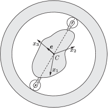
Figure 1: A system of two bodies coupled by a nonholonomic hinge.

In what follows we shall call this system a nonholonomic hinge (this problem was previously studied in [3, 4]).

Choose a moving coordinate system $Cx_{1}x_{2}x_{3}$ attached to the inner body. Then, if we denote the angular velocities of the inner body and the spherical shell by $\boldsymbol{\omega}$ and $\boldsymbol{\Omega}$, the constraint takes the form

$$\omega_{3}-\Omega_{3}=0.$$

In the absence of external forces the evolution of the angular velocities is governed by the following equations:

$$\dot{\Omega}_{1}=\omega_{3}(\Omega_{2}-\omega_{2}),\qquad\dot{\Omega}_{2}=\omega_{3}(\omega_{1}-\Omega_{1}),$$

$$I_{1}\dot{\omega}_{1}=(I_{2}-I_{3})\omega_{2}\omega_{3},\qquad I_{2}\dot{\omega}_{2}=(I_{3}-I_{1})\omega_{1}\omega_{3},$$

$$(I_{\text{s}}+I_{3})\dot{\omega}_{3}=I_{\text{s}}(\Omega_{1}\omega_{2}-\Omega_{2}\omega_{1})+(I_{1}-I_{2})\omega_{1}\omega_{2},$$ (11)

where ${\bf I}=\operatorname{diag}(I_{1},I_{2},I_{3})$ is the tensor of inertia of the inner body and $I_{\text{s}}$ is the tensor of inertia of the shell.

3.2 First integrals and the Poisson bracket

The system (11) possesses a standard invariant measure and conserves the energy:

$$d\Omega_{1}d\Omega_{2}d\omega_{1}d\omega_{2}d\omega_{3},\qquad E=\frac{1}{2}I_{\text{s}}(\Omega_{1}^{2}+\Omega_{2}^{2})+\frac{1}{2}\big{(}I_{1}\omega_{1}^{2}+I_{2}\omega_{2}^{2}+(I_{3}+I_{\text{s}})\omega_{3}^{2}\big{)}.$$

In order to use Theorem 2.4, we choose

$$\boldsymbol{u}=\frac{1}{\omega_{3}}\frac{\partial}{\partial\omega_{3}}$$

as $\boldsymbol{u}$. Then, if we denote the initial vector field (11) by $\boldsymbol{v}$, we obtain

$$[\boldsymbol{v},\boldsymbol{u}]=-\omega_{3}^{-1}\boldsymbol{v},\qquad\boldsymbol{u}(E)=2(I_{3}+I_{\text{s}}).$$

Thus, Theorem 2.4 holds and the system (11) can be represented in Hamiltonian form with a Poisson bracket in the variables $\boldsymbol{x}=(\Omega_{1},\Omega_{2},\omega_{1},\omega_{2},\omega_{3})$ of the form

$${\bf J}^{(2)}=\boldsymbol{v}\wedge\boldsymbol{u}=\begin{pmatrix}0&0&0&0&\Omega_{2}-\omega_{2}\\ 0&0&0&0&-(\Omega_{1}-\omega_{1})\vspace{1mm}\\ 0&0&0&0&\frac{I_{2}-I_{3}}{I_{1}}\omega_{2}\vspace{1mm}\\ 0&0&0&0&-\frac{I_{1}-I_{3}}{I_{2}}\omega_{1}\vspace{1mm}\\ *&*&*&*&0\end{pmatrix},$$

where the asterisks denote nonzero matrix entries resulting from the skew-symmetry condition ${\bf J}^{(2)}$. We note that even though the vector field $\boldsymbol{u}$ has a singularity when $\omega_{3}=0$, the resulting Poisson structure for the system is smooth.

The found Poisson bracket corresponds to the solvable Lie algebra. According to the classification of [37], this is the algebra $A^{spq}_{5,17}$ with $p=q=0$ (see [4] for details).

3.3 A flat inner body ($\boldsymbol{I_{3}=I_{1}+I_{2}}$)

In the case where the inner body is flat, i.e., $I_{3}=I_{1}+I_{2}$, for ${\bf J}^{(2)}$ we find all $k=n-\operatorname{rank}{\bf J}^{(2)}=3$ Casimir functions

$$C_{1}(\boldsymbol{x})=\omega_{1}^{2}+\omega_{2}^{2},\qquad C_{2}(\boldsymbol{x})=\Omega_{1}^{2}+(\omega_{2}-\Omega_{2})^{2},\qquad C_{3}(\boldsymbol{x})=\Omega_{2}^{2}+(\omega_{1}-\Omega_{1})^{2},$$

i.e., we obtain a case that is the simplest from the point of view of integrability.

Indeed, let us restrict the system (11) to the symplectic leaf by making the change of variables

$$\omega_{1}=c_{1}\cos\varphi,\qquad\omega_{2}=c_{1}\sin\varphi,$$

$$\Omega_{1}=c_{2}\cos(\varphi+c_{3}),\qquad\Omega_{2}=c_{1}\sin\varphi-c_{2}\sin(\varphi+c_{3}),$$

where $\varphi\in[0,2\pi)$ is the angular coordinate, and $c_{1}$, $c_{2}$, and $c_{3}$ parameterize the symplectic leaf

$$C_{1}(\boldsymbol{x})=\sqrt{c_{1}},\qquad C_{2}(\boldsymbol{x})=\sqrt{c_{2}},\qquad C_{3}(\boldsymbol{x})=c_{1}^{2}-2c_{1}c_{2}\cos c_{3}+c_{2}^{2}.$$

As a result, we obtain a system with one degree of freedom $(\varphi,\omega_{3})$ and a canonical Poisson bracket

$$\dot{\varphi}=\frac{\partial\widetilde{H}}{\partial\omega_{3}},\qquad\dot{\omega}_{3}=-\frac{\partial\widetilde{H}}{\partial\varphi},$$

$$\widetilde{H}=\frac{1}{2}\omega_{3}^{2}+\frac{c_{1}^{2}(I_{1}\cos^{2}\varphi+(I_{s}+I_{2})\sin^{2}\varphi)}{2(I_{s}+I_{1}+I_{2})}-\frac{I_{s}c_{1}c_{2}\sin(\varphi+c_{3})}{I_{s}+I_{s}+I_{2}}.$$ (12)

Some of its typical trajectories are shown in Fig. 2.

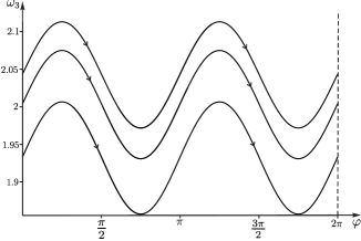
Figure 2: Typical trajectories $\eqref{Eqb03}$ for $I_{1}=2$, $I_{2}=3$, $I_{\text{s}}=1$, $c_{1}=1$, $c_{2}=2$, $c_{3}=\frac{\pi}{3}$.

3.4 The general case

In the general case the Poisson bracket possesses only two global Casimir functions [3, 4]

$$C_{1}(\boldsymbol{x})=I_{1}(I_{1}-I_{3})\omega_{1}^{2}+I_{2}(I_{2}-I_{3})\omega_{2}^{2},\qquad C_{2}(\boldsymbol{x})=(I_{1}\omega_{1}-I_{3}\Omega_{1})^{2}+(I_{2}\omega_{2}-I_{3}\Omega_{2})^{2},$$

while a third one does not exist in the general case (it is defined only locally).

Indeed, let us introduce coordinates on the symplectic leaf and assume that $I_{3}<I_{2}<I_{1}$:

$$\omega_{1}=\sqrt{\frac{c_{1}}{I_{1}(I_{1}-I_{3})}}\sin\varphi_{1},\qquad\omega_{2}=\sqrt{\frac{c_{1}}{I_{2}(I_{2}-I_{3})}}\cos\varphi_{1},$$

$$\Omega_{1}=\sqrt{\frac{I_{1}c_{1}}{I_{1}-I_{3}}}\frac{\sin\varphi_{1}}{I_{3}}-\sqrt{c_{2}}\frac{\sin\varphi_{2}}{I_{3}},\qquad\Omega_{2}=\sqrt{\frac{I_{2}c_{1}}{I_{2}-I_{3}}}\frac{\cos\varphi_{1}}{I_{3}}-\sqrt{c_{2}}\frac{\cos\varphi_{2}}{I_{3}},$$

where $\varphi_{1},\varphi_{2}\in[0,2\pi)$ and $C_{1}(\boldsymbol{x})=c_{1}$, $C_{2}(\boldsymbol{x})=c_{2}$.

In addition, we restrict the system to the level set of the energy integral $H=h$ by making the substitution

$$\omega_{3}(\varphi_{1},\varphi_{2})=\pm\sqrt{2h-\frac{2Q}{I_{3}^{2}(I_{3}+I_{\text{s}})}},$$

$$Q=\frac{I_{\text{s}}c_{2}}{2}+\frac{c_{1}}{2}\left(\frac{I_{\text{s}}I_{1}+I_{3}^{2}}{I_{1}-I_{3}}\sin^{2}\varphi_{1}+\frac{I_{\text{s}}I_{2}+I_{3}^{2}}{I_{2}-I_{3}}\cos^{2}\varphi_{1}\right)$$

$$\hphantom{Q=}{}-I_{\text{s}}\sqrt{c_{2}}\left(\sqrt{\frac{I_{1}c_{1}}{I_{1}-I_{3}}}\sin\varphi_{1}\sin\varphi_{2}+\sqrt{\frac{I_{2}c_{1}}{I_{2}-I_{3}}}\cos\varphi_{1}\cos\varphi_{2}\right).$$

As a result, the equations of motion can be represented as

$$\dot{\varphi}_{1}=k\omega_{3}(\varphi_{1},\varphi_{2}),\qquad\dot{\varphi}_{2}=\omega_{3}(\varphi_{1},\varphi_{2}),\qquad k^{2}=\frac{(I_{1}-I_{3})(I_{2}-I_{3})}{I_{1}I_{2}}.$$ (13)

In the case where $\omega_{3}(\varphi_{1},\varphi_{2})$ vanishes nowhere and $k$ is irrational, the trajectories (13) are rectilinear orbits on a torus (see Fig. 3).

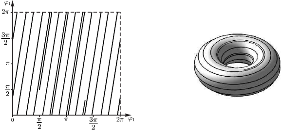
Figure 3: Trajectory (13) for $I_{1}=5.2$, $I_{2}=4.3$, $I_{3}=3.9$, $I_{\text{s}}=3.6$, $c_{1}=10$, $c_{2}=40$, $h=10$.

Such behavior is partially due to the fact that in the general case the missing solution (5) in the chosen (local) coordinates is represented as

$$\varphi_{1}-k\varphi_{2}={\rm const},$$

whence it follows that the projection of the symplectic leaf on ($\varphi_{1},\varphi_{2}$) is multi-valued.

A topological analysis of the system (11) is presented in [3]. In particular, it is shown that in addition to a torus there are two other types of integral surfaces: a sphere and a sphere with three handles (two-dimensional orientable surface of genus 3).

4 The Suslov problem

4.1 Equations of motion and first integrals

If we assume the spherical shell from the preceding example to be fixed, we obtain the so-called Suslov problem (in Vagner’s interpretation, see Fig. 4), which describes the motion of a rigid body with a fixed point subject to the nonholonomic constraint

$$(\boldsymbol{\omega},\boldsymbol{e})=0,$$

where $\boldsymbol{\omega}$ is the angular velocity of the body and $\boldsymbol{e}$ is the vector fixed in the body.

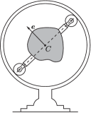
Figure 4: Realization of the Suslov problem.

Choose a moving coordinate system attached to the inner body, with one of the axes directed along $\boldsymbol{e}$. Then the tensor of inertia of the moving body can be represented as

$${\bf I}=\begin{pmatrix}I_{11}&0&I_{13}\\ 0&I_{22}&I_{23}\\ I_{13}&I_{23}&I_{33}\\ \end{pmatrix}.$$

In the axisymmetric potential field $U=U(\boldsymbol{\gamma})$ the problem reduces to the investigation of the following closed system of equations [10]:

$$I_{11}\dot{\omega}_{1}=-\omega_{2}(I_{13}\omega_{1}+I_{23}\omega_{2})+\gamma_{2}\frac{\partial U}{\partial\gamma_{3}}-\gamma_{3}\frac{\partial U}{\partial\gamma_{2}},$$

$$I_{22}\dot{\omega}_{2}=\omega_{1}(I_{13}\omega_{1}+I_{23}\omega_{2})+\gamma_{3}\frac{\partial U}{\partial\gamma_{1}}-\gamma_{1}\frac{\partial U}{\partial\gamma_{3}},$$

$$\dot{\gamma}_{1}=-\gamma_{3}\omega_{2},\qquad\dot{\gamma}_{2}=\gamma_{3}\omega_{1},\qquad\dot{\gamma}_{3}=\gamma_{1}\omega_{2}-\gamma_{2}\omega_{1},$$ (14)

where $\boldsymbol{\gamma}=(\gamma_{1},\gamma_{2},\gamma_{3})$ is the unit vector of the fixed coordinate system referred to the moving axes.

The system (14) conserves the energy and possesses the geometrical integral

$$E=\frac{1}{2}\big{(}I_{11}\omega_{1}^{2}+I_{22}\omega_{2}^{2}\big{)}+U,\qquad F=\gamma_{1}^{2}+\gamma_{2}^{2}+\gamma_{3}^{2}=1.$$

We now consider successively several particular cases (14).

4.2 Case $\boldsymbol{I_{13}=I_{23}=0}$ and $\boldsymbol{U=U(\gamma_{1},\gamma_{2})}$

Suppose that $I_{13}=I_{23}=0$, i.e., the constraint is imposed along the principal axis of inertia and the potential field has the form $U=U(\gamma_{1},\gamma_{2})$. Then the system (14) possesses a standard invariant measure.

Further, we introduce the vector field

$$\boldsymbol{u}=\frac{1}{\gamma_{3}}\frac{\partial}{\partial\gamma_{3}},$$

for which

$$[\boldsymbol{v},\boldsymbol{u}]=-\gamma_{3}^{-1}\boldsymbol{v},\qquad\boldsymbol{u}(F)=2.$$

Consequently, it follows from Theorem 2.4 that the initial system (14) can be represented in Hamiltonian form with the Poisson bracket

$${\bf J}^{(2)}=\boldsymbol{v}\wedge\boldsymbol{u}=\begin{pmatrix}0&0&0&0&-\frac{1}{I_{11}}\frac{\partial U}{\partial\gamma_{2}}\vspace{1mm}\\ 0&0&0&0&\frac{1}{I_{22}}\frac{\partial U}{\partial\gamma_{1}}\\ 0&0&0&0&-\omega_{2}\\ 0&0&0&0&\omega_{1}\\ *&*&*&*&0\end{pmatrix},$$

where the asterisks denote nonzero matrix entries resulting from the skew-symmetry condition ${\bf J}^{(2)}$.

Proposition 4.1.

In the general case, the bracket ${\bf J}^{(2)}$ possesses one global Casimir function – the energy integral $E$.

Proof 4.2.

First of all, we note that the Casimir functions ${\bf J}^{(2)}$ are simultaneously the integrals of the system

$$\dot{\omega}_{1}=-\frac{1}{I_{11}}\frac{\partial U}{\partial\gamma_{2}},\qquad\dot{\omega}_{2}=\frac{1}{I_{22}}\frac{\partial U}{\partial\gamma_{1}},\qquad\dot{\gamma}_{1}=-\omega_{2},\qquad\dot{\gamma}_{2}=\omega_{1},$$ (15)

which is Hamiltonian with Hamiltonian $E$ and the Poisson bracket

$$\{\omega_{1},\gamma_{2}\}=-\frac{1}{I_{1}},\qquad\{\omega_{2},\gamma_{1}\}=\frac{1}{I_{2}}.$$

Further, if we introduce new variables

$$p_{1}=\sqrt{I_{1}}\omega_{1},\qquad p_{2}=\sqrt{I_{2}}\omega_{2},\qquad q_{1}=\sqrt{I_{2}}\gamma_{1},\qquad q_{2}=\sqrt{I_{1}}\gamma_{2},$$

then the system (15) reduces to investigating a vector field with a canonical Poisson bracket and a Hamiltonian of the form

$$H=\frac{1}{2}(p_{1}^{2}+p_{2}^{2})+U\left(\frac{q_{1}}{I_{2}},\frac{q_{2}}{I_{1}}\right).$$ (16)

This is a natural system which describes the motion of a material point on a plane and in which, as is well known, there are generally no additional first integrals, and hence the resulting Poisson bracket has no remaining global Casimir functions.

Remark 4.3.

However, the system (16) has the well-know potentials $U$ for which there exist (one or two) additional integrals (and hence Casimir functions) of different degrees in momenta (see, e.g., the recent papers [34, 35] or [26, 27] for the Hénon–Heiles system).

4.3 Case $\boldsymbol{I_{13}\neq 0}$, $\boldsymbol{I_{23}\neq 0}$ and $\boldsymbol{U=(\boldsymbol{a},\boldsymbol{\gamma})}$

Now consider the more general situation $I_{13}\neq 0$, $I_{23}\neq 0$, but in the potential field $U=(\boldsymbol{a},\boldsymbol{\gamma})$.

In this case, the equations of motion are invariant under the transformation

$$\omega_{1}\rightarrow\lambda\omega_{1},\qquad\omega_{2}\rightarrow\lambda\omega_{2},\qquad\boldsymbol{\gamma}\rightarrow\lambda^{2}\boldsymbol{\gamma},\qquad dt\rightarrow\lambda^{-1}dt,$$

which is associated to the vector field

$$\widehat{\boldsymbol{u}}=\omega_{1}\frac{\partial}{\partial\omega_{1}}+\omega_{2}\frac{\partial}{\partial\omega_{2}}+2\gamma_{1}\frac{\partial}{\partial\omega_{1}}+2\gamma_{2}\frac{\partial}{\partial\omega_{2}}+2\gamma_{3}\frac{\partial}{\partial\omega_{3}},$$

for which we have

$$[\boldsymbol{u},\boldsymbol{v}]=\boldsymbol{v},\qquad\boldsymbol{u}(E)=2E.$$

Thus, the system under consideration can be represented in conformally Hamiltonian form with the Poisson bracket

$${\bf J}^{(2)}=\boldsymbol{v}\wedge\boldsymbol{u}.$$

In the case at hand, ${\bf J}^{(2)}$ has a rather cumbersome form, so we do not present it here explicitly. We note that it is cubic in the velocities $\boldsymbol{\omega}$.

Proposition 4.4.

In the general case, the system (14) has no invariant measure with smooth density in the potential field $U=(\boldsymbol{a},\boldsymbol{\gamma})$.

Proof 4.5.

In the potential field $U=(\boldsymbol{a},\boldsymbol{\gamma})$ the system (14) possesses a fixed point

$$\omega_{1}=0,\qquad\omega_{2}=-\frac{a_{3}}{I_{23}},\qquad\gamma_{1}=0,\qquad\gamma_{2}=1,\qquad\gamma_{3}=0$$

having a nonzero trace of the linearization matrix:

$$\frac{I_{13}}{I_{1}}\frac{\sqrt{a_{3}}}{\sqrt{I_{23}}}.$$

Consequently, the system considered has no invariant measure with smooth density [30, 31, 32] in a neighborhood of the fixed point.

Indeed, in this case the characteristic polynomial of the linearized system is represented as

$$P(\lambda)=\lambda^{2}\big{(}\lambda^{3}-c_{1}\lambda^{2}+c_{2}\lambda+c_{3}\big{)},$$

$$c_{1}=\frac{I_{13}\sqrt{a_{3}}}{I_{1}\sqrt{I_{23}}},\qquad c_{2}=\frac{a_{2}}{I_{1}}-\frac{I_{1}I_{2}+2I_{23}^{2}}{I_{23}I_{1}I_{2}}a_{3},\qquad c_{3}=\sqrt{a_{3}I_{23}}\left(\frac{I_{13}a_{3}}{I_{1}I_{23}^{2}}-\frac{2a_{1}}{I_{1}I_{2}}\right).$$

This polynomial is not reciprocal.

In this system, an analogous result was obtained for $U=0$ previously in [30]. Later, however, a singular invariant measure [10] was found in this case.

We also note that the pair of brackets that was constructed for the Suslov problem is defined in the extended phase space, as are the brackets described above.

$$\mathbb{R}^{2}\times\mathbb{R}^{3}=\{(\omega_{1},\omega_{2},\gamma_{1},\gamma_{2},\gamma_{3})\}.$$

Indeed, for these brackets the geometric integral $F=\gamma_{1}^{2}+\gamma_{2}^{2}+\gamma_{3}^{2}$ is not a Casimir function, so it is not clear how to restrict them to the actual phase space of the system

$$\mathbb{R}^{2}\times S^{2}=\{(\omega_{1},\omega_{2},\gamma_{1},\gamma_{2},\gamma_{3}),\gamma_{1}^{2}+\gamma_{2}^{2}+\gamma_{3}^{2}=1\}.$$

In view of the above discussion (at the end of Section 3.2), these brackets cannot provide any insight into the system’s properties.

Remark 4.6.

It may seem that a singular invariant measure with density having singularities in the considered family of fixed points is possible in this case too (see, e.g., Section 5). However, it is impossible to obtain a suitable solution of the Liouville equation in this case. Moreover, as numerical investigations show, this system may also have more complicated attracting sets – limit cycles. Numerical investigations also show that this system has no additional real-analytical integrals.

Remark 4.7.

A proof of the absence of meromorphic integrals for other (more particular) cases of the Suslov problem was obtained in [25, 36, 41]. The methods developed in these papers can be used in this case also, since the system (14) has a particular periodic solution which for $I_{13}=0$, $a_{1}=0$, and $a_{2}=0$ has the form

$$\omega_{1}(t)=2k\operatorname{cn}(t,k),\quad\omega_{2}(t)=0,\qquad\gamma_{1}(t)=0,\qquad\gamma_{2}(t)=-\frac{2I_{1}k}{a_{3}}\operatorname{sn}(t,k)\operatorname{dn}(t,k),$$

$$\gamma_{3}(t)=\frac{I_{1}}{a_{3}}\big{(}2k^{2}\operatorname{sn}^{2}(t,k)-1\big{)},\qquad H=I_{1}\big{(}2k^{2}-1\big{)},$$

where $\operatorname{sn}(t,k)$, $\operatorname{cn}(t,k)$, $\operatorname{dn}(t,k)$ are the elliptic Jacobi functions with parameter $k$.

Remark 4.8.

We note that in [10, 32] other cases of representation of the equations of the Suslov problem were found in Hamiltonian form, with a Poisson bracket of rank 4, which cannot be obtained with the help of the Hojman construction.

5 The Chaplygin sleigh

5.1 Equations of motion

The Chaplygin sleigh is a rigid body moving on a horizontal plane and supported at three points: two (absolutely) smooth posts and a knife edge such that the body cannot move perpendicularly to the plane of the wheel.

As a historical remark, we note that although the Chaplygin sleigh is usually linked to the works of Chaplygin [21] and Caratheodory [19], they were considered slightly earlier by Brill [40] as an example of the mechanism of a nonholonomic planimeter.

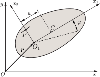
Figure 5: The Chaplygin sleigh on a plane.

In this case, the configuration space coincides with the group of motions of the plane ${\rm SE}(2)$. To parameterize it, we choose Cartesian coordinates $(x,y)$ of point $O_{1}$ (see Fig. 5) in the coordinate system $Oxy$ and the angle $\varphi$ of rotation of the axes $O_{1}x_{1}x_{2}$ relative to $Oxy$.

The motion of the Chaplygin sleigh in the variables $(v_{1},\omega,x,y,\varphi)$ is described by the equations (see [13] for details)

$$m\dot{v}_{1}=ma\omega^{2}-\frac{\partial U}{\partial x}\cos\varphi-\frac{\partial U}{\partial y}\sin\varphi,\qquad(I+ma^{2})\dot{\omega}=-ma\omega v_{1}-\frac{\partial U}{\partial\varphi},$$

$$\dot{x}=v_{1}\cos\varphi,\qquad\dot{y}=v_{1}\sin\varphi,\qquad\dot{\varphi}=\omega,$$ (17)

where $v_{1}$ is the projection of the velocity of point $O_{1}$ on the axis $O_{1}x_{1}$, and $m$ and $I$ are, respectively, the mass and the moment of inertia of the body, $a$ is the distance specifying the position of the knife edge, and $U$ is the potential of the external forces.

The system (17) conserves the energy integral

$$E=\frac{1}{2}\big{(}mv_{1}^{2}+\big{(}I+ma^{2}\big{)}\omega^{2}\big{)}+U.$$

Below we consider successively several particular cases.

5.2 The Chaplygin sleigh on a horizontal plane

Symmetry fields and invariant measure. In the absence of an external potential field $U=0$ the system (17) admits the symmetry group $SE(2)$ which is associated to the vector fields

$$\boldsymbol{u}_{x}=\frac{\partial}{\partial x},\qquad\boldsymbol{u}_{y}=\frac{\partial}{\partial y},\qquad\boldsymbol{u}_{\varphi}=\frac{\partial}{\partial\varphi},$$

which are symmetry fields.

Moreover, (17) possess a singular invariant measure

$$\omega^{-1}dv_{1}d\omega dxdyd\varphi.$$

Poisson bracket. We note that the system (17) is invariant under the transformation

$$v_{1}\rightarrow\lambda v_{1},\qquad\omega\rightarrow\lambda\omega,\qquad dt\rightarrow\lambda^{-1}dt,$$

which is associated to the vector field

$$\boldsymbol{u}=v_{1}\frac{\partial}{\partial v_{1}}+\omega\frac{\partial}{\partial\omega},$$

and

$$[\boldsymbol{u},\boldsymbol{v}]=\boldsymbol{v},\qquad\boldsymbol{u}(E)=2E,$$

where $\boldsymbol{v}$ is the initial vector field defined by the system (17).

Consequently, in the case $E\neq 0$ the system (17) is represented in Hamiltonian form

$$\dot{\boldsymbol{x}}={\bf J}^{(2)}\frac{\partial E}{\partial\boldsymbol{x}},\qquad\boldsymbol{x}=(v_{1},\omega,x,y,\varphi),$$

with the Poisson bracket

$${\bf J}^{(2)}=\frac{\boldsymbol{v}\wedge\boldsymbol{u}}{2E}=\begin{pmatrix}0&\frac{a\omega}{I+ma^{2}}&-\frac{v_{1}^{2}\cos\varphi}{mv_{1}^{2}+(I+ma^{2})\omega^{2}}&-\frac{v_{1}^{2}\sin\varphi}{mv_{1}^{2}+(I+ma^{2})\omega^{2}}&-\frac{\omega v_{1}}{mv_{1}^{2}+(I+ma^{2})\omega^{2}}\\ *&0&-\frac{v_{1}\omega\cos\varphi}{mv_{1}^{2}+(I+ma^{2})\omega^{2}}&-\frac{v_{1}\omega\sin\varphi}{mv_{1}^{2}+(I+ma^{2})\omega^{2}}&-\frac{\omega^{2}}{mv_{1}^{2}+(I+ma^{2})\omega^{2}}\\ *&*&0&0&0\\ *&*&*&0&0\\ *&*&*&*&0\end{pmatrix},$$

where the asterisks denote the matrix entries resulting from the skew-symmetry condition ${\bf J}^{(2)}$.

We examine in more detail a symplectic foliation which is defined by the bracket ${\bf J}^{(2)}$.

First of all, we note that the manifold

$$\mathcal{M}_{0}^{4}=\{(\omega,v_{1},x,y,\varphi)\,|\,\omega=0\}$$

defines a Poisson submanifold with the Casimir functions

$$C_{1}=\varphi,\qquad C_{2}=x\sin\varphi-y\cos\varphi.$$

Thus, the entire phase space of the system $\mathcal{M}^{5}$ is a union of three nonintersecting Poisson submanifolds

$$\mathcal{M}^{5}=\mathcal{M}^{5}_{+}\cup\mathcal{M}_{0}^{4}\cup\mathcal{M}^{5}_{-},$$

$$\mathcal{M}^{5}_{+}=\{(\omega,v_{1},x,y,\varphi)\,|\,\omega>0\},\qquad\mathcal{M}^{5}_{-}=\{(\omega,v_{1},x,y,\varphi)\,|\,\omega<0\}.$$

Let us consider $\mathcal{M}^{5}_{+}$ in more detail and pass from $(v_{1},\omega)$ to (polar) coordinates $(h,\psi)$:

$$v_{1}=Aah\cos\psi,\qquad\omega=h\sin\psi,\qquad A^{2}=1+\frac{I}{ma^{2}}>1,\qquad E=\frac{1}{2}mA^{2}a^{2}h^{2},$$

where $h\in(0,\infty)$ and $\psi\in(0,\pi)$. In the new variables $(\psi,x,y,\varphi,h)$ the Poisson bracket becomes

$${\bf J}^{(2)}=\begin{pmatrix}0&0&0&0&-hA^{-1}\sin\psi\\ 0&0&0&0&hAa\cos\psi\cos\varphi\\ 0&0&0&0&hAa\cos\psi\sin\varphi\\ 0&0&0&0&h\sin\psi\\ *&*&*&*&0\end{pmatrix}.$$ (18)

As a result, the Casimir functions (18) have the form

$$C_{1}=A\psi+\varphi,\qquad C_{2}=x+A^{2}a\int_{\psi^{*}}^{\psi}\tan(\xi)\cos(A\xi-C_{1})d\xi,$$

$$C_{3}=y-A^{2}a\int_{\psi^{*}}^{\psi}\tan(\xi)\sin(A\xi-C_{1})d\xi,$$ (19)

where $\psi^{*}\in(0,\pi)$.

The level surface of the Casimir function $C_{1}={\rm const}$ foliates the domain $\mathcal{M}^{5}_{+}$ into four-dimensional surfaces. The projection of each such surface into the three-dimensional space

$$S^{1}\times\mathbb{R}^{2}_{+}=\{(\varphi,\omega,v_{1})\,|\,\omega>0\}$$

is a ruled surface (similar to a helicoid). Its equation can be represented in the following parametric form

$$v_{1}=Aah\cos\left(\frac{\varphi+C_{1}}{A}\right),\qquad\omega=h\sin\left(\frac{\varphi+C_{1}}{A}\right),\qquad\varphi=\varphi.$$ (20)

In the definition (20) the periodicity in $\varphi$ should, of course, be taken into account (see Fig. 6).

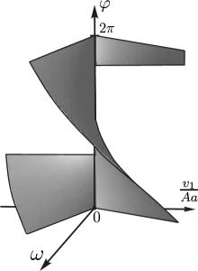
Figure 6: Characteristic surface defined by the Casimir function $C_{1}$ in the domain $\mathcal{M}^{5}_{+}$ for $C_{1}=2$ and $A=3$.

Proceeding in a similar way for $\mathcal{M}^{5}_{-}$, it is easy to check that relations (19) also define the Casimir functions with the only difference that $\psi^{*}\in(\pi,2\pi)$.

The second Poisson bracket. In this case it turns out that when $E\neq 0$, by Proposition 2.6, the system (17) can be represented in conformally Hamiltonian form

$$\dot{\boldsymbol{x}}=(2E)^{(-1)}{\bf J}^{(4)}\frac{\partial E}{\partial\boldsymbol{x}},$$

with a Poisson bracket of rank 4 using the symmetry fields as follows: $\widehat{\boldsymbol{u}}_{x}$ and $\widehat{\boldsymbol{u}}_{y}$

$${\bf J}^{(4)}=\boldsymbol{v}\wedge\boldsymbol{u}+\boldsymbol{u}_{x}\wedge\boldsymbol{u}_{y}=\!\!\begin{pmatrix}0&a\omega^{3}+\frac{ma}{I+ma^{2}}\omega v_{1}^{2}&-v_{1}^{2}\cos\varphi&-v_{1}^{2}\sin\varphi&-\omega v_{1}\\ *&0&-v_{1}\omega\cos\varphi&-v_{1}\omega\sin\varphi&-\omega^{2}\\ *&*&0&1&0\\ *&*&*&0&0\\ *&*&*&*&0\end{pmatrix}.$$

Remark 5.1.

We note that the Jacobi identity for the matrix $\frac{{\bf J}^{(4)}}{E}$ does not hold.

In this case, $\omega=0$ defines the Poisson submanifold ${\bf J}^{(4)}$ on which ${\operatorname{rank}{\bf J}^{(4)}=2}$, and the Casimir functions are

$$C_{1}=\varphi,\qquad C_{2}=Aa(x\sin\varphi-y\cos\varphi)-h^{-1}.$$

In the remaining region of the phase space $\overline{{\bf J}}$ possesses the only Casimir function

$$C_{1}=A\psi+\varphi,\qquad\tan\varphi=\frac{v_{2}}{Aa\omega}.$$

The bracket ${\bf J}^{(4)}$ was obtained previously in the initial coordinates $(v_{1},\omega,x,y,\varphi)$ in [13].

5.3 The Chaplygin sleigh on an inclined plane

Below we consider the motion of the Chaplygin sleigh on an inclined plane. We direct the axis $Ox$ along the line of maximum slope, then

$$U=m\mu(x+a\cos\varphi),\qquad\mu=g\sin\chi,$$

where $\chi$ is the angle of inclination of the plane to the horizon. In this case, the energy integral has the form

$$E=\frac{I+ma^{2}}{2}\omega^{2}+\frac{mv_{1}^{2}}{2}+m\mu(x+a\cos\varphi).$$

Moreover, two symmetry fields are preserved in the system (17)

$$\boldsymbol{u}_{x}=\frac{\partial}{\partial x},\qquad\boldsymbol{u}_{y}=\frac{\partial}{\partial y}.$$

Since $\boldsymbol{u}_{x}(E)=m\mu$, Theorem 1 applies to this system.

As a result, its equations of motion are represented in Hamiltonian form with the Poisson bracket ${\bf J}^{(2)}$ of rank 2:

$${\bf J}^{(2)}=\boldsymbol{v}\wedge\boldsymbol{u}_{x}=\begin{pmatrix}0&\omega&0&0&0\\ *&0&-v_{1}\sin\varphi&\mu\cos\varphi-a\omega^{2}&\frac{ma}{I+ma^{2}}(\omega v_{1}-\mu\sin\varphi)\\ *&*&0&0&0\\ *&*&*&0&0\\ *&*&*&*&0\end{pmatrix},$$

where $\boldsymbol{v}$ is the initial vector field defined by the system (17).

In [13] it is shown that the dynamics of this system, which is noncompact, has a complicated, seemingly random behavior, leading to the absence of an invariant measure and global analytic Casimir functions in this system.

6 Conclusion

Thus, in this paper it has been shown that the Hojman construction (using conformal symmetry fields) allows one to obtain Poisson brackets for various nonholonomic systems. As a rule, the resulting Poisson brackets do not possess a maximal rank, and in the general case a smooth invariant measure and global Casimir functions may be absent for these brackets. Nevertheless, as shown in [3], the above-mentioned Poisson brackets can be useful to investigate stability problems.

Acknowledgments

Section 3 was prepared by A.V. Borisov under the RSF grant No. 15-12-20035. Section 2 was written by I.S. Mamaev within the framework of the state assignment for institutions of higher education. The work of I.A. Bizyaev (Sections 4 and 5) was supported by RFBR grant No. 15-31-50172. The authors thank A.V. Tsiganov and A.V. Bolsinov for useful discussions and the referees for numerous comments, which have contributed to the improvement of this paper.

References

- [1] Benenti S., A ‘user-friendly’ approach to the dynamical equations of non-holonomic systems, SIGMA 3 (2007), 036, 33 pages, math.DS/0703043.
- [2] Benenti S., The non-holonomic double pendulum: an example of non-linear non-holonomic system, Regul. Chaotic Dyn. 16 (2011), 417–442.
- [3] Bizyaev I.A., Bolsinov A.V., Borisov A.V., Mamaev I.S., Topology and bifurcations in nonholonomic mechanics, Internat. J. Bifur. Chaos Appl. Sci. Engrg. 25 (2015), 1530028, 21 pages.
- [4] Bizyaev I.A., Borisov A.V., Mamaev I.S., The dynamics of nonholonomic systems consisting of a spherical shell with a moving rigid body inside, Regul. Chaotic Dyn. 19 (2014), 198–213.
- [5] Bizyaev I.A., Kozlov V.V., Homogeneous systems with quadratic integrals, Lie–Poisson quasi-brackets, and the Kovalevskaya method, Sb. Math. 206 (2015), 29–54.
- [6] Bizyaev I.A., Tsiganov A.V., On the Routh sphere problem, J. Phys. A: Math. Theor. 46 (2013), 085202, 11 pages, arXiv:1210.7903.
- [7] Bolsinov A.V., Borisov A.V., Mamaev I.S., Hamiltonization of non-holonomic systems in the neighborhood of invariant manifolds, Regul. Chaotic Dyn. 16 (2011), 443–464.
- [8] Bolsinov A.V., Borisov A.V., Mamaev I.S., Geometrisation of Chaplygin’s reducing multiplier theorem, Nonlinearity 28 (2015), 2307–2318, arXiv:1405.5843.
- [9] Borisov A.V., Kazakov A.O., Sataev I.R., The reversal and chaotic attractor in the nonholonomic model of Chaplygin’s top, Regul. Chaotic Dyn. 19 (2014), 718–733.
- [10] Borisov A.V., Kilin A.A., Mamaev I.S., Hamiltonicity and integrability of the Suslov problem, Regul. Chaotic Dyn. 16 (2011), 104–116.
- [11] Borisov A.V., Kilin A.A., Mamaev I.S., The problem of drift and recurrence for the rolling Chaplygin ball, Regul. Chaotic Dyn. 18 (2013), 832–859.
- [12] Borisov A.V., Mamaev I.S., Conservation laws, hierarchy of dynamics and explicit integration of nonholonomic systems, Regul. Chaotic Dyn. 13 (2008), 443–490.
- [13] Borisov A.V., Mamaev I.S., The dynamics of a Chaplygin sleigh, J. Appl. Math. Mech. 73 (2009), 156–161.
- [14] Borisov A.V., Mamaev I.S., Symmetries and reduction in nonholonomic mechanics, Regul. Chaotic Dyn. 20 (2015), 553–604.
- [15] Borisov A.V., Mamaev I.S., Bizyaev I.A., The hierarchy of dynamics of a rigid body rolling without slipping and spinning on a plane and a sphere, Regul. Chaotic Dyn. 18 (2013), 277–328.
- [16] Borisov A.V., Mamaev I.S., Bizyaev I.A., The Jacobi integral in nonholonomic mechanics, Regul. Chaotic Dyn. 20 (2015), 383–400.
- [17] Cantrijn F., Cortés J., de León M., Martín de Diego D., On the geometry of generalized Chaplygin systems, Math. Proc. Cambridge Philos. Soc. 132 (2002), 323–351, math.DS/0008141.
- [18] Cantrijn F., de León M., Martín de Diego D., On almost-Poisson structures in nonholonomic mechanics, Nonlinearity 12 (1999), 721–737.
- [19] Carathéodory C., Der Schlitten, Z. Angew. Math. Mech. 13 (1933), 71–76.
- [20] Cariñena J.F., Guha P., Rañada M.F., Quasi-Hamiltonian structure and Hojman construction, J. Math. Anal. Appl. 332 (2007), 975–988.
- [21] Chaplygin S.A., On the theory of motion of nonholonomic systems. The reducing-multiplier theorem, Regul. Chaotic Dyn. 13 (2008), 369–376.
- [22] Fassò F., Giacobbe A., Sansonetto N., Periodic flows, rank-two Poisson structures, and nonholonomic mechanics, Regul. Chaotic Dyn. 10 (2005), 267–284.
- [23] Fassò F., Sansonetto N., Conservation of energy and momenta in nonholonomic systems with affine constraints, Regul. Chaotic Dyn. 20 (2015), 449–462, arXiv:1505.01172.
- [24] Fedorov Yu.N., García-Naranjo L.C., Marrero J.C., Unimodularity and preservation of volumes in nonholonomic mechanics, J. Nonlinear Sci. 25 (2015), 203–246, arXiv:1304.1788.
- [25] Fedorov Yu.N., Maciejewski A.J., Przybylska M., The Poisson equations in the nonholonomic Suslov problem: integrability, meromorphic and hypergeometric solutions, Nonlinearity 22 (2009), 2231–2259, arXiv:0902.0079.
- [26] Grammaticos B., Dorizzi B., Ramani A., Hamiltonians with high-order integrals and the “weak-Painlevé” concept, J. Math. Phys. 25 (1984), 3470–3473.
- [27] Hénon M., Heiles C., The applicability of the third integral of motion: Some numerical experiments, Astronom. J. 69 (1964), 73–79.
- [28] Hojman S.A., The construction of a Poisson structure out of a symmetry and a conservation law of a dynamical system, J. Phys. A: Math. Gen. 29 (1996), 667–674.
- [29] Konyaev A.Yu., Classification of Lie algebras with generic orbits of dimension 2 in the coadjoint representation, Sb. Math. 205 (2014), 45–62.
- [30] Kozlov V.V., On the existence of an integral invariant of a smooth dynamic system, J. Appl. Math. Mech. 51 (1987), 420–426.
- [31] Kozlov V.V., Invariant measures of the Euler–Poincaré equations on Lie algebras, Funct. Anal. Appl. 22 (1988), 58–59.
- [32] Kozlov V.V., On the integration theory of equations of nonholonomic mechanics, Regul. Chaotic Dyn. 7 (2002), 161–176, nlin.SI/0503027.
- [33] Kozlov V.V., Yaroshchuk V.A., On invariant measures of Euler–Poincaré equations on unimodular groups, Mosc. Univ. Mech. Bull. (1993), no. 2, 45–50.
- [34] Maciejewski A.J., Przybylska M., Yoshida H., Necessary conditions for super-integrability of Hamiltonian systems, Phys. Lett. A 372 (2008), 5581–5587.
- [35] Maciejewski A.J., Przybylska M., Yoshida H., Necessary conditions for classical super-integrability of a certain family of potentials in constant curvature spaces, J. Phys. A: Math. Theor. 43 (2010), 382001, 15 pages, arXiv:1004.3854.
- [36] Mahdi A., Valls C., Analytic non-integrability of the Suslov problem, J. Math. Phys. 53 (2012), 122901, 8 pages.
- [37] Patera J., Sharp R.T., Winternitz P., Zassenhaus H., Invariants of real low dimension Lie algebras, J. Math. Phys. 17 (1976), 986–994.
- [38] Tsiganov A.V., One invariant measure and different Poisson brackets for two non-holonomic systems, Regul. Chaotic Dyn. 17 (2012), 72–96, arXiv:1106.1952.
- [39] Tsiganov A.V., On the Poisson structures for the nonholonomic Chaplygin and Veselova problems, Regul. Chaotic Dyn. 17 (2012), 439–450.
- [40] von Brill A., Vorlesungen zur Einführung in die Mechanik raumerfüllender Massen, B.G. Teubner, Berlin, 1909.
- [41] Ziglin S.L., On the absence of an additional first integral in the special case of the G.K. Suslov problem, Russ. Math. Surv. 52 (1997), 434–435.