On the reachable states for the boundary control of the heat equation

Abstract.

We are interested in the determination of the reachable states for the boundary control of the one-dimensional heat equation. We consider either one or two boundary controls. We show that reachable states associated with square integrable controls can be extended to analytic functions on some square of $\mathbb{C}$, and conversely, that analytic functions defined on a certain disk can be reached by using boundary controls that are Gevrey functions of order 2. The method of proof combines the flatness approach with some new Borel interpolation theorem in some Gevrey class with a specified value of the loss in the uniform estimates of the successive derivatives of the interpolating function.

1. Introduction

The null controllability of the heat equation has been extensively studied since the seventies. After the pioneering work [11] in the one-dimensional case using biorthogonal families, sharp results were obtained in the N-dimensional case by using elliptic Carleman estimates [20] or parabolic Carleman estimates [12]. An exact controllability to the trajectories was also derived, even for nonlinear systems [12].

By contrast, the issue of the exact controllability of the heat equation (or of a more general semilinear parabolic equation) is not well understood. For the sake of simplicity, let us consider the following control system

$$\psi_{t}-\psi_{xx}=0, x\in(0,1),\ t\in(0,T),$$ (1.1)

$$\psi(0,t)=h_{0}(t), t\in(0,T),$$ (1.2)

$$\psi(1,t)=h_{1}(t), t\in(0,T),$$ (1.3)

$$\psi(x,0)=\psi_{0}(x), x\in(0,1),$$ (1.4)

where $\psi_{0}\in L^{2}(0,1)$, and $h_{0},h_{1}\in L^{2}(0,T)$.

As (1.1)-(1.4) is null controllable, there is no loss of generality is assuming that $\psi_{0}\equiv 0$. A state $\psi_{1}$ is said to be reachable (from $0$ in time $T$) if we can find two control inputs $h_{0},h_{1}\in L^{2}(0,T)$ such that the solution $\psi$ of (1.1)-(1.4) satisfies

$$\psi(x,T)=\psi_{1}(x),\quad\forall x\in(0,1).$$ (1.5)

Let $A\psi:=\psi^{\prime\prime}$ with domain $D(A):=H^{2}(0,1)\cap H^{1}_{0}(0,1)\subset L^{2}(0,1)$, and let $e_{n}(x)=\sqrt{2}\sin(n\pi x)$ for $n\geq 1$ and $x\in(0,1)$. As is well known, $(e_{n})_{n\geq 1}$ is an orthonormal basis in $L^{2}(0,1)$ constituted of eigenfunctions of $A$. Decompose $\psi_{1}$ as

$$\psi_{1}(x)=\sum_{n=1}^{\infty}c_{n}e_{n}(x)=\sum_{n=1}^{\infty}c_{n}\sqrt{2}\sin(n\pi x).$$ (1.6)

Then, from [11], if we have for some $\varepsilon>0$

$$\sum_{n=1}^{\infty}|c_{n}|n^{-1}e^{(1+\varepsilon)n\pi}<\infty,$$ (1.7)

then $\psi_{1}$ is a reachable terminal state. Note that the condition (1.7) implies that

1. the function $\psi_{1}$ is analytic in $D(0,1+\varepsilon):=\{z\in\mathbb{C};\ |z|<1+\varepsilon\}$, for the series in (1.6) converges uniformly in $\overline{D(0,r)}$ for all $r<1+\varepsilon$;

2. $$\sum_{n=1}^{\infty}|c_{n}|^{2}n^{2k}<\infty,\quad\forall k\in\mathbb{N}$$ (1.8)

   (that is, $\psi_{1}\in\cap_{k\geq 0}D(A^{k})$), and hence

   $$\psi_{1}^{(2n)}(0)=\psi_{1}^{(2n)}(1)=0,\quad\forall n\in\mathbb{N}.$$ (1.9)

More recently, it was proved in [10] that any state $\psi_{1}$ decomposed as in (1.6) is reachable if

$$\sum_{n\geq 1}|c_{n}|^{2}ne^{2n\pi}<\infty,$$ (1.10)

which again implies (1.8) and (1.9).

It turns out that (1.9) is a very conservative condition, which excludes most of the usual analytic functions. As a matter of fact, the only polynomial function satisfying (1.9) is the null one. On the other hand, the condition (1.9) is not very natural, for there is no reason that $h_{0}(T)=h_{1}(T)=0$. We shall see that the only condition required for $\psi_{1}$ to be reachable is the analyticity of $\psi_{1}$ on a sufficiently large open set in $\mathbb{C}$.

Notations: If $\Omega$ is an open set in $\mathbb{C}$, we denote by $H(\Omega)$ the set of holomorphic (complex analytic) functions $f:\Omega\to\mathbb{C}$.

The following result gathers together some of the main results contained in this paper.

Theorem 1.1.

1. Let $z_{0}=\frac{1}{2}$. If $\psi_{1}\in H(D(z_{0},R/2))$ with $R>R_{0}:=e^{(2e)^{-1}}\sim 1.2$, then $\psi_{1}$ is reachable from $0$ in any time $T>0$. Conversely, any reachable state belongs to $H(\{z=x+iy;\ |x-\frac{1}{2}|+|y|<\frac{1}{2}\})$.
2. If $\psi_{1}\in H(D(0,R))$ with $R>R_{0}$ and $\psi_{1}$ is odd, then $\psi_{1}$ is reachable from 0 in any time $T>0$ with only one boundary control at $x=1$ (i.e. $h_{0}\equiv 0$). Conversely, any reachable state with only one boundary control at $x=1$ is odd and it belongs to $H(\{z=x+iy;\ |x|+|y|<1\})$.

Thus, for given $a\in\mathbb{R}$, the function $\psi_{1}(x):=[(x-\frac{1}{2})^{2}+a^{2}]^{-1}$ is reachable if $|a|>R_{0}/2\sim 0.6$, and it is not reachable if $|a|<1/2$.

Figure 1 is concerned with the reachable states associated with two boundary controls at $x=0,1$: any reachable state can be extended to the red square as a (complex) analytic function; conversely, the restriction to $[0,1]$ of any analytic function on a disc containing the blue one is a reachable state.

Figure 1. $\{|x-\frac{1}{2}|+|y|<\frac{1}{2}\}$ (red) and $D(z_{0},\frac{R_{0}}{2})$ (blue)

Figure 2 is concerned with the reachable states associated with solely one boundary control at $x=1$: any reachable state can be extended to the red square as an analytic (odd) function; conversely, the restriction to $[0,1]$ of any analytic (odd) function on a disc containing the blue one is a reachable state.

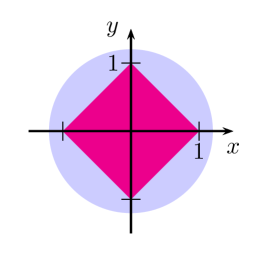
Figure 2. $\{|x|+|y|<1\}$ (red) and $D(0,R_{0})$ (blue)

The proof of Theorem 1.1 does not rely on the study of a moment problem as in [11], or on the duality approach involving some observability inequality for the adjoint problem [10, 12]. It is based on the flatness approach introduced in [18, 19] for the motion planning of the one-dimensional heat equation between “prepared” states (e.g. the steady states). Since then, the flatness approach was extended to deal with the null controllability of the heat equation on cylinders, yielding accurate numerical approximations of both the controls and the trajectories [24, 27], and to give new null controllability results for parabolic equations with discontinuous coefficients that may be degenerate or singular [25].

For system (1.1)-(1.4) with $h_{0}\equiv 0$, the flatness approach consists in expressing the solution $\psi$ (resp. the control) in the form

$$\psi(x,t)=\sum_{i\geq 0}z^{(i)}(t)\frac{x^{2i+1}}{(2i+1)!},\quad h_{1}(t)=\sum_{i=0}^{\infty}\frac{z^{(i)}(t)}{(2i+1)!},$$ (1.11)

where $z\in C^{\infty}([0,T])$ is designed in such a way that: (i) the series in (1.11) converges for all $t\in[0,T]$; (ii) $z^{(i)}(0)=0$ for all $i\geq 0$; and (iii)

$$\sum_{i=0}^{\infty}z^{(i)}(T)\frac{x^{2i+1}}{(2i+1)!}=\psi_{1}(x)\quad\forall x\in(0,1).$$

If $\psi_{1}$ is analytic in an open neighborhood of $\{z;|z|\leq 1\}$ and $\psi_{1}$ is odd, then $\psi_{1}$ can be written as

$$\psi_{1}(x)=\sum_{i=0}^{\infty}d_{i}\frac{x^{2i+1}}{(2i+1)!}$$ (1.12)

with

$$|d_{i}|\leq C\frac{(2i)!}{R^{2i}}$$ (1.13)

for some $C>0$ and $R>1$. Thus $\psi_{1}$ is reachable provided that we can find a function $z\in C^{\infty}([0,T])$ fulfilling the conditions

$$z^{(i)}(0) = 0,\quad\forall i\geq 0,$$ (1.14)

$$z^{(i)}(T) = d_{i},\quad\forall i\geq 0,$$ (1.15)

$$|z^{(i)}(t)| \leq C\left(\frac{\rho}{R}\right)^{2i}(2i)!\quad\forall i\geq 0,\ \forall t\in[0,T],$$ (1.16)

for some constants $C>0$ and $\rho\in(1,R)$.

A famous result due to Borel [5] asserts that one can find a function $z\in C^{\infty}([0,T])$ satisfying (1.15). The condition (1.14) can easily be imposed by multiplying $z$ by a convenient cutoff function. Thus, the main difficulty in this approach comes from condition (1.16), which tells us that the derivatives of the function $z$ (Gevrey of order 2) grow in almost the same way as the $d_{i}$’s for $t\neq T$.

The Borel interpolation problem in Gevrey classes (or in more general non quasianalytic classes) has been considered e.g. in [8, 17, 26, 28, 29, 31]. The existence of a constant $\rho>1$ (that we shall call the loss) for which (1.16) holds for any $R>0$ and any sequence $(d_{i})_{i\geq 0}$ as in (1.13), was proved in those references. Explicit values of $\rho$ were however not provided so far. On the other hand, to the best knowledge of the authors, the issue of the determination of the optimal value of $\rho$, for any sequence $(d_{i})_{i\geq 0}$ or for a given sequence $(d_{i})_{i\geq 0}$ as in (1.13), was not addressed so far. We stress that this issue is crucial here, for the convergence of the series in (1.11) requires $R>\rho$: sharp results for the reachable states require sharp results for $\rho$.

There are roughly two ways to derive a Borel interpolation theorem in a Gevrey class. The complex variable approach, as e.g. in [17, 26, 33], results in the construction of an interpolating function which is complex analytic in a sector of $\mathbb{C}$. It will be used here to derive an interpolation result without loss, but for a restricted class of sequences $(d_{i})_{i\geq 0}$ (see below Theorem 3.9). The real variable approach, as in [1, 28], yields an infinitely differentiable function of the real variable $x$ only. In [28], Petzsche constructed an interpolating function with the aid of a cut-off function obtained by repeated convolutions of step functions [15, Thm 1.3.5]. Optimizing the constants in Petzsche’s construction of the interpolating function, we shall obtain an interpolation result with as a loss $\rho=R_{0}\sim 1.2$ (see below Proposition 3.7).

The paper is outlined as follows. Section 2 is concerned with the necessary conditions for a state to be reachable (Theorem 2.1). Section 3 is mainly concerned with the interpolation problem (1.15)-(1.16). An interpolation result obtained by the real variable approach with as a loss $\rho=R_{0}\sim 1.2$ is given in Proposition 3.7. This interpolation result is next applied to the problem of the determination of the set of reachable states, first with only one control (the other homogeneous boundary condition being of Neumann or of Dirichlet type), and next with two boundary controls of Robin type. The section ends with the application of the complex variable approach to Borel interpolation problem. An interpolation result without loss is derived (Theorem 3.9), thanks to which we can exhibit reachable states for (1.1)-(1.4) analytic in $D(1/2,R)$ with $R>1/2$ arbitrarily close to $1/2$. The paper ends with a section providing some concluding remarks and some open questions. Two appendices give some additional material.

Notations: A function $y\in C^{\infty}([t_{1},t_{2}])$ is said to be Gevrey of order $s\geq 0$ on $[t_{1},t_{2}]$ if there exist some constants $C,R>0$ such that

$$|y^{(p)}(t)|\leq C\displaystyle\frac{p!^{s}}{R^{p}},\quad\forall p\in\mathbb{N},\ \forall t\in[t_{1},t_{2}].$$

The set of functions Gevrey of order $s$ on $[t_{1},t_{2}]$ is denoted $G^{s}([t_{1},t_{2}])$.

A function $\theta\in C^{\infty}([x_{1},x_{2}]\times[t_{1},t_{2}])$ is said to be Gevrey of order $s_{1}$ in $x$ and $s_{2}$ in $t$ on $[x_{1},x_{2}]\times[t_{1},t_{2}]$ if there exist some constants $C,R_{1},R_{2}>0$ such that

$$|\partial_{x}^{p_{1}}\partial_{t}^{p_{2}}\theta(x,t)|\leq C\frac{(p_{1}!)^{s_{1}}(p_{2}!)^{s_{2}}}{R_{1}^{p_{1}}R_{2}^{p_{2}}}\quad\forall p_{1},p_{2}\in\mathbb{N},\ \forall(x,t)\in[x_{1},x_{2}]\times[t_{1},t_{2}].$$

The set of functions Gevrey of order $s_{1}$ in $x$ and $s_{2}$ in $t$ on $[x_{1},x_{2}]\times[t_{1},t_{2}]$ is denoted $G^{s_{1},s_{2}}([x_{1},x_{2}]\times[t_{1},t_{2}])$.

2. Necessary conditions for reachability

In this section, we are interested in deriving necessary conditions for a state function to be reachable from 0. More precisely, we assume given $T>0$ and we consider any solution $\psi$ of the heat equation in $(-1,1)\times(0,T)$:

$$\psi_{t}-\psi_{xx}=0,\quad x\in(-1,1),\ t\in(0,T).$$ (2.1)

Let us introduce the rectangle

$${\mathcal{R}}:=\{z=x+iy\in\mathbb{C};\ |x|+|y|<1\}.$$

The following result gives a necessary condition for a state to be reachable, regardless of the kind of boundary control that is applied. It extends slightly a classical result due to Gevrey for continuous Dirichlet controls (see [7, 13]).

Theorem 2.1.

Let $T>0$ and let $\psi$ denote any solution of (2.1). Then $\psi(.,T^{\prime})\in H({\mathcal{R}})$ for all $T^{\prime}\in(0,T)$.

Proof.

Pick any $\varepsilon>0$ with $\varepsilon<\min(1,T/2)$. From (2.1) and a classical interior regularity result (see e.g. [16, Thm 11.4.12]), we know that $\psi\in G^{1,2}([-1+\varepsilon,1-\varepsilon]\times[\varepsilon,T-\varepsilon])$. Let $h_{0}(t):=\psi(-1+\varepsilon,t+\varepsilon)$, $h_{1}(t):=\psi(1-\varepsilon,t+\varepsilon)$, $u_{0}(x):=\psi(x,\varepsilon)$, and $u(x,t):=\psi(x,t+\varepsilon)$. Then $u\in G^{1,2}([-1+\varepsilon,1-\varepsilon]\times[0,T-2\varepsilon])$ is the unique solution to the following initial-boundary-value problem

$$u_{t}-u_{xx}=0, x\in(-1+\varepsilon,1-\varepsilon),\ t\in(0,T-2\varepsilon),$$ (2.2)

$$u(-1+\varepsilon,t)=h_{0}(t), t\in(0,T-2\varepsilon),$$ (2.3)

$$u(1-\varepsilon,t)=h_{1}(t), t\in(0,T-2\varepsilon),$$ (2.4)

$$u(x,0)=u_{0}(x), x\in(-1+\varepsilon,1-\varepsilon).$$ (2.5)

Let

$$K(x,t):=\frac{1}{\sqrt{4\pi t}}\exp(-\frac{x^{2}}{4t}),\quad x\in\mathbb{R},\ t>0,$$

denote the fundamental solution of the heat equation. By [7, Theorem 6.5.1] (with some obvious change to fit our $x-$domain), the solution $u$ of (2.2)-(2.5) can be written as

$$u(x,t)=v(x,t)-2\int_{0}^{t}\frac{\partial K}{\partial x}(x+1-\varepsilon,t-s)\phi_{0}(s)ds+2\int_{0}^{t}\frac{\partial K}{\partial x}(x-1+\varepsilon,t-s)\phi_{1}(s)ds$$

where

$$v(x,t)=\int_{-\infty}^{\infty}K(x-\xi,t)\tilde{u}_{0}(\xi)d\xi,$$

$\tilde{u}_{0}$ denoting any smooth, bounded extension of $u_{0}$ outside of $-1+\varepsilon\leq x\leq 1-\varepsilon$, and where the pair $(\phi_{1},\phi_{2})$ solves the system

$$h_{0}(t) = v(-1+\varepsilon,t)+\phi_{0}(t)+2\int_{0}^{t}\frac{\partial K}{\partial x}(-2+2\varepsilon,t-s)\phi_{1}(s)ds,$$ (2.6)

$$h_{1}(t) = v(1-\varepsilon,t)+\phi_{1}(t)-2\int_{0}^{t}\frac{\partial K}{\partial x}(2-2\varepsilon,t-s)\phi_{0}(s)ds.$$ (2.7)

Since $h_{0},h_{1},v(-1+\varepsilon,.),v(1-\varepsilon,.)\in C([0,T-2\varepsilon])$, it is well known (see e.g. [7]) that the system (2.6)-(2.7) has a unique solution $(\phi_{0},\phi_{1})\in C([0,T-2\varepsilon])^{2}$. Furthermore, for any $t\in(0,T-2\varepsilon)$, we have that

• $v(z,t)$ is an entire analytic function in $z$ by [7, Theorem 10.2.1];

• $\int_{0}^{t}\frac{\partial K}{\partial x}(z+1-\varepsilon,t-s)\phi_{0}(s)ds$ is analytic in the variable $z$ in the domain $\{z=x+iy;\ x>-1+\varepsilon,\ |y|<|x+1-\varepsilon|\}$ by [7, Theorem 10.4.1];

• $\int_{0}^{t}\frac{\partial K}{\partial x}(z-1+\varepsilon,t-s)\phi_{1}(s)ds$ is analytic in the variable $z$ in the domain $\{z=x+iy;\ x<1-\varepsilon,\ |y|<|x-1+\varepsilon|\}$ by [7, Corollary 10.4.1].

It follows that for $0<t<T-2\varepsilon$, $z\to u(z,t)$ is analytic in the domain

$${\mathcal{R}}_{\varepsilon}:=\{z=x+iy;\ |x|+|y|<1-\varepsilon\}.$$

Pick any $T^{\prime}\in(0,T)$, and pick $\varepsilon<\min(1,T/2,T^{\prime},T-T^{\prime})$. Then $T^{\prime}-\varepsilon\in(0,T-2\varepsilon)$ and $z\to\psi(z,T^{\prime})=u(z,T^{\prime}-\varepsilon)$ is analytic in ${\mathcal{R}}_{\varepsilon}$. As $\varepsilon$ can be chosen arbitrarily small, we conclude that $z\to\psi(z,T^{\prime})$ is analytic in $\mathcal{R}$. ∎

Pick any $(\alpha,\beta)\in\mathbb{R}^{2}\setminus\{(0,0)\}$, and consider the system

$$\psi_{t}-\psi_{xx}=0,\quad x\in(0,1),\ t\in(0,T),$$ (2.8)

$$\alpha\psi(1,t)+\beta\psi_{x}(1,t)=h(t), t\in(0,T),$$ (2.9)

$$\psi(x,0)=\psi_{0}(x), x\in(0,1),$$ (2.10)

supplemented with either the homogeneous Dirichlet condition

$$\psi(0,t)=0,\quad t\in(0,T),$$ (2.11)

or the homogeneous Neumann condition

$$\psi_{x}(0,t)=0,\quad t\in(0,T).$$ (2.12)

Then we have the following result.

Corollary 2.2.

Let $T>0$, $\psi_{0}\in L^{2}(0,1)$ and $h\in L^{2}(0,T)$. Then the solution $\psi$ of (2.8)-(2.10) and (2.11) (resp. (2.8)-(2.10) and (2.12)) is such that for all $T^{\prime}\in(0,T)$, the map $z\to\psi(z,T^{\prime})$ is analytic in $\mathcal{R}$ and odd (resp. even).

Proof.

Let $\psi$ denote the solution of (2.8)-(2.10) and (2.11). Extend $\psi$ to $(-1,1)\times(0,T)$ as an odd function in $x$; that is, set

$$\psi(x,t)=\psi(-x,t),\quad x\in(-1,0),\ t\in(0,T).$$

Then it is easily seen that $\psi$ is smooth in $(-1,1)\times(0,T)$ and that it satisfies (2.1). The conclusion follows from Theorem 2.1. (Note that $\psi(z,T^{\prime})$ is odd in $z$ for $z\in(-1,1)$, and also for all $z\in\mathcal{R}$ by analytic continuation.) When $\psi$ denotes the solution of (2.8)-(2.10) and (2.12), we proceed similarly by extending $\psi$ to $(-1,1)\times(0,T)$ as an even function in $x$. ∎

3. Sufficient conditions for reachability

3.1. Neumann control

Let us consider first the Neumann control of the heat equation. We consider the control system

$$\theta_{t}-\theta_{xx}=0, x\in(0,1),\ t\in(0,T),$$ (3.1)

$$\theta_{x}(0,t)=0,\ \theta_{x}(1,t)=h(t), t\in(0,T),$$ (3.2)

$$\theta(x,0)=\theta_{0}(x), x\in(0,1).$$ (3.3)

We search a solution in the form

$$\theta(x,t)=\sum_{i\geq 0}\frac{x^{2i}}{(2i)!}y^{(i)}(t)$$ (3.4)

where $y\in G^{2}([0,T])$.

Proposition 3.1.

Assume that for some constants $M>0$, $R>1$, we have

$$|y^{(i)}(t)|\leq M\frac{(2i)!}{R^{2i}}\qquad\forall i\geq 0,\ \forall t\in[0,T].$$ (3.5)

Then the function $\theta$ given in (3.4) is well defined on $[0,1]\times[0,T]$, and

$$\theta\in G^{1,2}([0,1]\times[0,T]).$$ (3.6)

Remark 3.2.

Proposition 3.1 is sharp as far as the value of $R$ is concerned. It improves some result in [18, p. 46-47], where the same conclusion was obtained under the assumption

$$|y^{(i)}(t)|\leq M\frac{i!^{2}}{\tilde{R}^{i}}\qquad\forall i\geq 0,\ \forall t\in[0,T],$$ (3.7)

with $\tilde{R}>4$. Using Stirling formula, we see that $(2i)!/(i!)^{2}\sim 2^{2i}/\sqrt{\pi i}$ so that (3.5) is equivalent to

$$|y^{(i)}(t)|\leq\frac{M}{\sqrt{\pi i}}\frac{i!^{2}}{(\frac{R^{2}}{4})^{i}}\qquad\forall i\geq 0,\ \forall t\in[0,T].$$ (3.8)

Our result is valid whenever $\tilde{R}:=R^{2}/4>1/4$.

Proof.

We need to prove some uniform estimate for the series of the derivatives

$$\partial_{t}^{m}\partial_{x}^{n}[\frac{x^{2i}}{(2i)!}y^{(i)}(t)]=\frac{x^{2i-n}}{(2i-n)!}y^{(i+m)}(t)$$

for $2i-n\geq 0$, $x\in[0,1]$, and $t\in[0,T]$. Fix $m,n\in\mathbb{N}$, $i\in\mathbb{N}$ with $2i-n\geq 0$ and let $j:=2i-n\geq 0$, $N:=n+2m\geq n$ (hence $2i+2m=j+N$). We infer from (3.5) that

$$\left|\frac{y^{(i+m)}(t)}{(2i-n)!}\right|\leq M\frac{(2i+2m)!}{(2i-n)!\,R^{2i+2m}}=M\frac{(j+N)!}{j!R^{j+N}}\cdot$$

Let

$$S:=\sum_{i,\,2i-n\geq 0}\big{|}\partial_{t}^{m}\partial_{x}^{n}[\frac{x^{2i}}{(2i)!}y^{(i)}]\big{|}.$$

Then

$$S \leq \sum_{i,\,2i-n\geq 0}|\frac{y^{(i+m)}(t)}{(2i-n)!}|$$

$$\leq M\sum_{j\geq 0}\frac{(j+1)(j+2)\cdots(j+N)}{R^{j+N}}$$

$$= M\sum_{k\geq 0}\ \ \sum_{kN\leq j<(k+1)N}\frac{(j+1)(j+2)\cdots(j+N)}{R^{j+N}}$$

$$\leq M\sum_{k\geq 0}N\frac{[(k+2)N]^{N}}{R^{(k+1)N}}$$

$$= MN^{N+1}\sum_{k\geq 0}\left(\frac{k+2}{R^{k+1}}\right)^{N}.$$

Pick any number $\sigma\in(0,1)$. Since $R>1$, $(k+2)/(R^{1-\sigma})^{k+1}\to 0$ as $k\to+\infty$, and hence

$$a:=\sup_{k\geq 0}\frac{k+2}{(R^{1-\sigma})^{k+1}}<\infty.$$

We infer that

$$\left(\frac{k+2}{R^{k+1}}\right)^{N}\leq\left(\frac{a}{R^{\sigma(k+1)}}\right)^{N},$$

and hence

$$\sum_{k\geq 0}\left(\frac{k+2}{R^{k+1}}\right)^{N}\leq a^{N}\sum_{k\geq 0}R^{-N\sigma(k+1)}=\frac{a^{N}}{R^{N\sigma}-1}\cdot$$

It follows that

$$S\leq MN^{N+1}\frac{a^{N}}{R^{N\sigma}-1}\leq M^{\prime}\left(\frac{ae}{R^{\sigma}}\right)^{N}N!\sqrt{N}$$

for some constant $M^{\prime}>0$, where we used Stirling formula $N!\sim(N/e)^{N}\sqrt{2\pi N}$ in the last inequality. Since $N=n+2m$, we have that

$$N!\leq 2^{n+2m}n!(2m)!\leq C\frac{2^{n+4m}}{\sqrt{m}}n!(m!)^{2},$$

where we used again Stirling formula. We conclude that

$$S\leq CM^{\prime}\left(\frac{ae}{R^{\sigma}}\right)^{n+2m}2^{n+4m}n!(m!)^{2}\sqrt{\frac{n+2m}{m}}\leq M^{\prime\prime}\frac{(m!)^{2}}{R_{1}^{m}}\frac{n!}{R_{2}^{n}}$$

for some positive constants $M^{\prime\prime}$, $R_{1}$ and $R_{2}$. (We noticed that $\sqrt{n+2m}\leq C\rho^{n+m}$ for $\rho>1$ and some $C>0$.) This proves that the series of derivatives $\partial_{t}^{m}\partial_{x}^{n}[x^{2i}y^{(i)}(t)/(2i)!]$ is uniformly convergent on $[0,1]\times[0,T]$ for all $m,n\geq 0$, so that $\theta\in C^{\infty}([0,1]\times[0,T])$ and it satisfies

$$|\partial_{t}^{m}\partial_{x}^{n}\theta(x,t)|\leq M^{\prime\prime}\frac{(m!)^{2}}{R_{1}^{m}}\frac{n!}{R_{2}^{n}}\qquad\forall m,n\in\mathbb{N},\ \forall(x,t)\in[0,1]\times[0,T],$$

as desired. The proof of Proposition 3.1 is complete. ∎

Theorem 3.3.

Pick any $\theta_{T}\in G^{1}([0,1])$ written as

$$\theta_{T}(x)=\sum_{i\geq 0}c_{2i}\frac{x^{2i}}{(2i)!}$$ (3.9)

with

$$|c_{2i}|\leq M\frac{(2i)!}{R^{2i}}$$ (3.10)

for some $M>0$ and $R>R_{0}:=e^{(2e)^{-1}}>1.2$. Then for any $T>0$ and any $R^{\prime}\in(R_{0},R)$, one can pick a function $y\in G^{2}([0,T])$ such that

$$y^{(i)}(0)=0\quad \forall i\geq 0,$$ (3.11)

$$y^{(i)}(T)=c_{2i}\quad \forall i\geq 0,$$ (3.12)

$$|y^{(i)}(t)|\leq M^{\prime}(\frac{R^{\prime}}{R})^{2i}(2i)!\quad \forall t\in[0,T],\ \forall i\geq 0$$ (3.13)

for some constant $M^{\prime}>0$. Thus, the control input $h(t):=\sum_{i\geq 0}\frac{y^{(i)}(t)}{(2i-1)!}$ is Gevrey of order 2 on $[0,T]$ by Proposition 3.1, and it steers the solution $\theta$ of (3.1)-(3.3) from $0$ at $t=0$ to $\theta_{T}$ at $t=T$.

Proof.

Using Proposition 3.1, it is clearly sufficient to prove the existence of a function $y\in C^{\infty}([0,T])$ satisfying (3.11)-(3.13). To do it, we shall need several lemmas. The first one comes from [15, Theorem 1.3.5].

Lemma 3.4.

Let $a_{0}\geq a_{1}\geq a_{2}\geq\cdots>0$ be a sequence such that $a:=\sum_{j=0}^{\infty}a_{j}<\infty$. Then there exists $u\in C_{0}^{\infty}(\mathbb{R})$ such that

$$u\geq 0,\ \int_{\mathbb{R}}u(x)dx=1,\ \textrm{Supp }u\subset[0,a],$$

and $$|u^{(k)}(x)|\leq 2^{k}(a_{0}a_{1}\cdots a_{k})^{-1},\qquad\forall k\geq 0,\ \forall x\in\mathbb{R}.$$

The following lemma improves slightly Lemma 3.4 as far as the estimates of the derivatives are concerned.

Lemma 3.5.

Let $a_{0}\geq a_{1}\geq a_{2}\geq\cdots>0$ be a sequence such that $a:=\sum_{j=0}^{\infty}a_{j}<\infty$. Then for any $\delta>0$, there exist $v\in C_{0}^{\infty}(\mathbb{R})$ and $M>0$ such that

$$v\geq 0,\ \int_{\mathbb{R}}v(x)dx=1,\ \textrm{Supp }v\subset[0,a],$$

and $$|v^{(k)}(x)|\leq M\delta^{k}(a_{0}a_{1}\cdots a_{k})^{-1},\qquad\forall k\geq 0,\ \forall x\in\mathbb{R}.$$

Proof of Lemma 3.5: For any given $k_{0}\in\mathbb{N}$, let

$$\kappa:=a\big{(}(k_{0}+1)a_{k_{0}}+\sum_{k>k_{0}}a_{k}\big{)}^{-1},$$

and

$$\tilde{a}_{k}:=\left\{\begin{array}[]{ll}\kappa a_{k_{0}}&\textrm{ if }0\leq k\leq k_{0},\\ \kappa a_{k}&\textrm{ if }k>k_{0}.\end{array}\right.$$

Since the sequence $(a_{k})_{k}$ is nonincreasing and the series $\sum_{k\geq 0}a_{k}$ is convergent, it follows from Pringsheim’s theorem (see [14]) that

$$ka_{k}\to 0\qquad\textrm{ as }k\to+\infty.$$

Therefore, we may pick $k_{0}\in\mathbb{N}$ so that

$$\kappa>\frac{2}{\delta}\cdot$$

Note that $\sum_{k\geq 0}\tilde{a}_{k}=a$. Pick a function $v\in C_{0}^{\infty}(\mathbb{R})$ as in Lemma 3.4 and associated with the sequence $(\tilde{a}_{k})_{k\geq 0}$; that is,

$$v\geq 0,\ \int_{\mathbb{R}}v(x)dx=1,\ \textrm{Supp }v\subset[0,a],$$

and $$|v^{(k)}(x)|\leq 2^{k}(\tilde{a}_{0}\tilde{a}_{1}\cdots\tilde{a}_{k})^{-1},\qquad\forall k\geq 0,\ \forall x\in\mathbb{R}.$$

Then, for any $k\geq k_{0}$,

$$|v^{(k)}(x)| \leq (\kappa a_{k_{0}})^{-(k_{0}+1)}2^{k}\kappa^{-(k-k_{0})}(a_{k_{0}+1}\cdots a_{k})^{-1}$$

$$\leq \kappa^{-1}(\frac{2}{\kappa})^{k}\frac{a_{0}a_{1}\cdots a_{k_{0}}}{a_{k_{0}}^{k_{0}+1}}\big{(}\prod_{i=0}^{k}a_{i}\big{)}^{-1}.$$

Thus

$$|v^{(k)}(x)|\leq M_{1}\delta^{k}(a_{0}\cdots a_{k})^{-1},$$

where

$$M_{1}:=\kappa^{-1}\frac{a_{0}a_{1}\cdots a_{k_{0}-1}}{a_{k_{0}}^{k_{0}}}\cdot$$

Finally, for $0\leq k\leq k_{0}$ and $x\in\mathbb{R}$

$$|v^{(k)}(x)|\leq 2^{k}(\kappa a_{k_{0}})^{-(k+1)}\leq M_{2}\delta^{k}(a_{0}\cdots a_{k})^{-1}$$

with

$$M_{2}:=\sup_{0\leq k\leq k_{0}}(\frac{2}{\delta})^{k}\frac{a_{0}a_{1}\cdots a_{k}}{(\kappa a_{k_{0}})^{k+1}}\cdot$$

We conclude that

$$|v^{(k)}(x)|\leq M\delta^{k}(a_{0}\cdots a_{k})^{-1},\qquad\forall k\geq 0,\ \forall x\in\mathbb{R}$$

with $M:=\sup(M_{1},M_{2})$.∎

Corollary 3.6.

For any sequence $(a_{k})_{k\geq 1}$ satisfying $a_{1}\geq a_{2}\geq\cdots>0$ and $\sum_{k\geq 1}a_{k}<\infty$ and for any $\delta>0$, there exists a function $\varphi\in C^{\infty}_{0}(\mathbb{R})$ with $\textrm{Supp }\varphi\subset[-a,a]$, $0\leq\varphi\leq 1$, $\varphi^{(p)}(0)=\delta_{p}^{0}$ and

$$|\varphi^{(k)}(x)|\leq C\delta^{k}(a_{1}\cdots a_{k})^{-1}\quad\forall k\geq 0,\ \forall x\in\mathbb{R},$$

with the convention that $a_{1}\cdots a_{k}=1$ if $k=0$.

Indeed, there exist by Lemma 3.5 a function $v\in C_{0}^{\infty}(\mathbb{R})$ and a number $C>0$ such that

$$v\geq 0,\ \int_{\mathbb{R}}v(x)dx=1,\ \textrm{Supp }v\subset[0,a],$$

and $$|v^{(k)}(x)|\leq C\delta^{k}(a_{1}\cdots a_{k+1})^{-1},\qquad\forall k\geq 0,\ \forall x\in\mathbb{R}.$$

Note that $v^{(k)}(a)=0$ $\forall k\geq 0$. Let

$$\varphi(x):=\int_{-\infty}^{a-|x|}v(s)ds.$$

Clearly, $\varphi\in C_{0}^{\infty}(\mathbb{R})$, $0\leq\varphi\leq 1$, $\textrm{ Supp }\varphi\subset[-a,a]$, $\varphi^{(j)}(0)=\delta_{j}^{0}$, and

$$|\varphi^{(k)}(x)|\leq C\frac{\delta^{k-1}}{a_{1}\cdots a_{k}}\leq C^{\prime}\frac{\delta^{k}}{a_{1}\cdots a_{k}}\qquad\forall k\geq 1,\ \forall x\in\mathbb{R}.$$

Proposition 3.7.

Pick any sequence $(a_{k})_{k\geq 0}$ satisfying $1=a_{0}\geq a_{1}\geq a_{2}\geq\cdots>0$ and

$$a:=\sum_{k\geq 1}a_{k}<\infty,$$

$$pa_{p}+\sum_{k>p}a_{k}\leq Apa_{p}\qquad\forall p\geq 1,$$

for some constant $A\in(0,+\infty)$. Let $M_{q}:=(a_{0}\cdots a_{q})^{-1}$ for $q\geq 0$. Then for any sequence of real numbers $(d_{q})_{q\geq 0}$ such that

$$|d_{q}|\leq CH^{q}M_{q}\quad\forall q\geq 0,$$ (3.14)

for some $H>0$ and $C>0$, and for any $\tilde{H}>e^{e^{-1}}H$, there exists a function $f\in C^{\infty}(\mathbb{R})$ such that

$$f^{(q)}(0) = d_{q},\quad\forall q\geq 0,$$ (3.15)

$$|f^{(q)}(x)| \leq C\tilde{H}^{q}M_{q}\quad\forall q\geq 0,\ \forall x\in\mathbb{R}.$$ (3.16)

Proof.

We follow closely [28]. Let $m_{q}:=1/a_{q}$ for $q\geq 0$, so that $M_{q}=m_{0}\cdots m_{q}$. For any given $h>0$, we set $\tilde{a}_{k}:=h^{-1}a_{k}$ for all $k\geq 0$, so that

$$h^{-1}a=\sum_{k\geq 1}\tilde{a}_{k},$$

$$p\tilde{a}_{p}+\sum_{k>p}\tilde{a}_{k}\leq Ap\tilde{a}_{p}=Ap/(hm_{p})\qquad\forall p\geq 1.$$

By Corollary 3.6 applied to the sequence $(\tilde{a}_{q})_{q\geq 1}$, there is a function $\varphi\in C^{\infty}_{0}(\mathbb{R})$ such that $\textrm{Supp }\varphi\subset[-h^{-1}a,h^{-1}a]$, $0\leq\varphi\leq 1$, $\varphi^{(j)}(0)=\delta_{j}^{0}$ and

$$|\varphi^{(j)}(x)|\leq C(\delta h)^{j}M_{j}\qquad\forall j\geq 0.$$

Set $\zeta_{0}(x)=\varphi_{0}(x):=\varphi(x)$. Applying for any $p\in\mathbb{N}^{*}$ Corollary 3.6 to the sequence

$$\hat{a}_{k}:=\left\{\begin{array}[]{ll}\tilde{a}_{p}&\textrm{ if }1\leq k\leq p,\\ \tilde{a}_{k}&\textrm{ if }k\geq p+1,\end{array}\right.$$

we may also pick a function $\varphi_{p}\in C^{\infty}(\mathbb{R})$ with $\varphi_{p}\subset[-Ap/(hm_{p}),Ap/(hm_{p})]$, $0\leq\varphi_{p}\leq 1$, $\varphi_{p}^{(j)}(0)=\delta_{j}^{0}$ and

$$|\varphi_{p}^{(j)}(x)|\leq\left\{\begin{array}[]{ll}C(\delta hm_{p})^{j}&\textrm{ if }0\leq j\leq p,\\ C(\delta h)^{j}m_{p}^{p}\frac{M_{j}}{M_{p}}&\textrm{ if }j>p.\end{array}\right.$$

We set $\zeta_{p}(x):=\varphi_{p}(x)\frac{x^{p}}{p!}$, so that $\zeta_{p}^{(j)}(0)=\delta_{j}^{p}$. To estimate $\zeta_{p}^{(j)}$ for $p\geq 1$ and $j\geq 0$, we distinguish two cases.
(i) For $0\leq j\leq p$, we have

$$|\zeta_{p}^{(j)}(x)| \leq \sum_{i=0}^{j}\left(\begin{array}[]{c}j\\ i\end{array}\right)|\varphi_{p}^{(i)}(x)\frac{x^{p-j+i}}{(p-j+i)!}|$$

$$\leq C\sum_{i=0}^{j}\left(\begin{array}[]{c}j\\ i\end{array}\right)(\delta hm_{p})^{i}\left(\frac{A}{hm_{p}}\right)^{p-j+i}\frac{p^{p-j+i}}{(p-j+i)!}$$

$$\leq C\frac{M_{j}}{M_{p}}(\frac{A}{h})^{p}\sum_{i=0}^{j}\left(\begin{array}[]{c}j\\ i\end{array}\right)(\delta h)^{i}\left(\frac{h}{A}\right)^{j-i}\frac{m_{j+1}\cdots m_{p}}{m_{p}^{p-j}}\frac{p^{p-j+i}}{(p-j+i)!}$$

$$\leq C\frac{M_{j}}{M_{p}}(\frac{Ae}{h})^{p}\sum_{i=0}^{j}\left(\begin{array}[]{c}j\\ i\end{array}\right)(\delta h)^{i}\left(\frac{h}{Ae}\right)^{j-i}\left(\frac{p}{p-j+i}\right)^{p-j+i}$$

where we used Stirling’s formula and the fact that the sequence $(m_{i})_{i\geq 0}$ is nondecreasing in the last inequality. Elementary computations show that the function $x\in[0,p]\to\left(\frac{p}{p-x}\right)^{p-x}\in\mathbb{R}$ reaches its greatest value for $x=p(1-e^{-1})$, and hence

$$\left(\frac{p}{p-j+i}\right)^{p-j+i}\leq e^{\frac{p}{e}}.$$

We conclude that

$$|\zeta_{p}^{(j)}(x)|\leq C\frac{M_{j}}{M_{p}}(\frac{Ae^{1+e^{-1}}}{h})^{p}\left(\delta h+\frac{h}{Ae}\right)^{j}.$$ (3.21)

(ii) For $j>p$, we have

$$|\zeta_{p}^{(j)}(x)| \leq \sum_{i=j-p}^{j}\left(\begin{array}[]{c}j\\ i\end{array}\right)|\varphi_{p}^{(i)}(x)\frac{x^{p-j+i}}{(p-j+i)!}|$$

$$\leq C\sum_{\tiny\begin{array}[]{c}j-p\leq i\leq j\\ \textrm{and }i\leq p\end{array}}\left(\begin{array}[]{c}j\\ i\end{array}\right)(\delta hm_{p})^{i}\left(\frac{A}{hm_{p}}\right)^{p-j+i}\frac{p^{p-j+i}}{(p-j+i)!}$$

$$+\,C\sum_{\tiny\begin{array}[]{c}j-p\leq i\leq j\\ \textrm{and }i\geq p+1\end{array}}\left(\begin{array}[]{c}j\\ i\end{array}\right)(\delta h)^{i}m_{p}^{p}\frac{M_{i}}{M_{p}}\left(\frac{A}{hm_{p}}\right)^{p-j+i}\frac{p^{p-j+i}}{(p-j+i)!}=:CS_{1}+CS_{2}.$$

We infer from the computations in the case $0\leq j\leq p$ that

$$S_{1}\leq C\frac{M_{j}}{M_{p}}(\frac{Ae^{1+e^{-1}}}{h})^{p}\left(\delta h+\frac{h}{Ae}\right)^{j}.$$

For $S_{2}$, we notice that

$$\frac{M_{i}}{M_{p}}m_{p}^{j-i}=\frac{M_{j}}{M_{p}}\frac{m_{p}^{j-i}m_{p+1}\cdots m_{i}}{m_{p+1}\cdots m_{j}}\leq\frac{M_{j}}{M_{p}}$$

where we used again the fact that the sequence $(m_{j})_{j\geq 0}$ is nondecreasing. Thus

$$S_{2} \leq C\frac{M_{j}}{M_{p}}(\frac{Ae}{h})^{p}\sum_{\tiny\begin{array}[]{c}j-p\leq i\leq j\\ \textrm{and }i\geq p+1\end{array}}\left(\begin{array}[]{c}j\\ i\end{array}\right)(\delta h)^{i}\left(\frac{h}{Ae}\right)^{j-i}\left(\frac{p}{p-j+i}\right)^{p-j+i}$$

$$\leq C\frac{M_{j}}{M_{p}}(\frac{Ae^{1+e^{-1}}}{h})^{p}\left(\delta h+\frac{h}{Ae}\right)^{j}.$$

We conclude that (3.21) is valid also for $j>p$. Clearly, (3.21) is also true for $p=0$ and $j\geq 0$.

Let the sequence $(d_{q})_{q\geq 0}$ and the number $H$ be as in (3.14). Pick $\delta>0$ and $h>0$ such that

$$h=(1+\delta)Ae^{1+e^{-1}}H,$$

and

$$\delta h+\frac{h}{Ae}=(1+\delta)(\delta Ae+1)e^{e^{-1}}H<\tilde{H}.$$

Let $f(x):=\sum_{p\geq 0}d_{p}\zeta_{p}(x)$. Then $f\in C^{\infty}(\mathbb{R})$, and for all $x\in\mathbb{R}$ and all $j\geq 0$

$$|f^{(j)}(x)| \leq \sum_{p\geq 0}|d_{p}\zeta_{p}^{(j)}(x)|$$

$$\leq C\sum_{p\geq 0}(H^{p}M_{p})\frac{M_{j}}{M_{p}}(\frac{Ae^{1+e^{-1}}}{h})^{p}\left(\delta h+\frac{h}{Ae}\right)^{j}$$

$$\leq C\sum_{p\geq 1}(1+\delta)^{-p}\tilde{H}^{j}M_{j}$$

$$\leq C\tilde{H}^{j}M_{j}.$$

Thus (3.16) holds, and (3.15) is obvious.

To ensure that the support of $f$ can be chosen as small as desired, we need the following

Lemma 3.8.

Let $-\infty<T_{1}<T_{2}<\infty$, $1<\sigma<s$, and let $f\in G^{s}([T_{1},T_{2}])$ and $g\in G^{\sigma}([T_{1},T_{2}])$; that is

$$|f^{(n)}(t)| \leq C\frac{n!^{s}}{R^{n}}\qquad\forall t\in[T_{1},T_{2}],\ \forall n\geq 0,$$ (3.26)

$$|g^{(n)}(t)| \leq C^{\prime}\frac{n!^{\sigma}}{\rho^{n}}\qquad\forall t\in[T_{1},T_{2}],\ \forall n\geq 0,$$ (3.27)

where $C,C^{\prime},R$ and $\rho$ are some positive constants. Then $fg\in G^{s}([T_{1},T_{2}])$ with the same $R$ as for $f$; that is, we have for some constant $C^{\prime\prime}>0$

$$|(fg)^{(n)}(t)|\leq C^{\prime\prime}\frac{n!^{s}}{R^{n}}\qquad\forall t\in[T_{1},T_{2}],\ \forall n\geq 0.$$ (3.28)

Proof.

From Leibniz’ rule and (3.26)-(3.27), we have that

$$|(fg)^{(n)}(t)|=\left|\sum_{j=0}^{n}\left(\begin{array}[]{c}n\\ j\end{array}\right)f^{(j)}(t)g^{(n-j)}(t)\right|\leq CC^{\prime}\sum_{j=0}^{n}\left(\begin{array}[]{c}n\\ j\end{array}\right)\frac{j!^{s}(n-j)!^{\sigma}}{R^{j}\rho^{n-j}}.$$ (3.29)

We claim that

$$\left(\begin{array}[]{c}n\\ j\end{array}\right)\frac{j!^{s}(n-j)!^{\sigma}}{R^{j}\rho^{n-j}}\leq\tilde{C}\frac{n!^{s}}{2^{n-j}R^{n}}\cdot$$ (3.30)

Indeed, (3.30) is equivalent to

$$j!^{s-1}(n-j)!^{\sigma-1}\leq\tilde{C}(\frac{\rho}{2R})^{n-j}n!^{s-1}$$ (3.31)

and to prove (3.31), we note that, since $1<\sigma<s$,

$$j!^{s-1}(n-j)!^{\sigma-1}=(n-j)!^{\sigma-s}(j!(n-j)!)^{s-1}\leq\tilde{C}(\frac{\rho}{2R})^{n-j}n!^{s-1}$$

for some constant $\tilde{C}>0$ and all $0\leq j\leq n$. It follows from (3.29)-(3.30) that

$$|(fg)^{(n)}(t)|\leq 2CC^{\prime}\tilde{C}\frac{n!^{s}}{R^{n}}\qquad\forall t\in[T_{1},T_{2}],\ \forall n\geq 0.$$

∎

Multiplying $f$ by a cutoff function $g\in C^{\infty}_{0}(\mathbb{R})$ with $g(x)=1$ for $|x|<a/2$, $\textrm{Supp }(g)\subset[-a,a]$, and $g\in G^{\sigma}([-a,a])$ for some $1<\sigma<2$, we can still assume that $\textrm{Supp }f\subset[-a,a]$. The proof of Proposition 3.7 is complete. ∎

We apply Proposition 3.7 with $d_{q}=c_{2q}$ for all $q\geq 0$, $a_{0}=1$, $a_{p}=[2p(2p-1)]^{-1}$ for $p\geq 1$, so that $M_{p}=(2p)!$, $H=R^{-2}$, $\tilde{H}\in(e^{e^{-1}}H,(R^{\prime}/R)^{2})$. Let $f$ be as in (3.15)-(3.16), and pick $g\in G^{\sigma}([0,T])$ with $1<\sigma<2$, $g^{(i)}(0)=0$ for all $i\geq 0$, $g(T)=1$, and $g^{(i)}(T)=0$ for all $i\geq 1$. Set finally

$$y(t)=f(t-T)g(t),\quad t\in[0,T].$$

Since by (3.16)

$$|f^{(i)}(t)|\leq C\tilde{H}^{i}(2i)!\leq C\frac{(4\tilde{H})^{i}i!^{2}}{\sqrt{i+1}}\quad\forall t\in\mathbb{R},$$

we infer from Lemma 3.8 that

$$|y^{(i)}(t)|\leq C(4\tilde{H})^{i}i!^{2}\leq C\sqrt{i+1}\tilde{H}^{i}(2i)!\leq C(\frac{R^{\prime}}{R})^{2i}(2i)!\qquad\forall i\in[0,T],$$

i.e. (3.13) holds. The properties (3.11) and (3.12) are clearly satisfied. The proof of Theorem 3.3 is complete. ∎

The following result, proved by using the complex variable approach, gives a Borel interpolation result without loss, but for a restricted class of sequences $(d_{n})_{n\geq 0}$.

Theorem 3.9.

Let $(d_{n})_{n\geq 0}$ be a sequence of complex numbers such that

$$|d_{n}|\leq M\frac{(2n)!}{R^{2n}}\quad\forall n\in\mathbb{N}$$ (3.32)

for some constants $M>0$ and $R>1$, and such that the function

$$g(z):=\sum_{n\geq 0}\frac{d_{n+1}}{n!(n+1)!}z^{n},\quad|z|<R^{2}/4,$$ (3.33)

can be extended as an analytic function in an open neighborhood of $\mathbb{R}_{-}$ in $\mathbb{C}$ with

$$|g^{(n)}(z)|\leq C|g^{(n)}(0)|\quad\forall z\in\mathbb{R}_{-},\ \forall n\in\mathbb{N}$$ (3.34)

for some constant $C>0$. Let $-\infty<T_{1}<T_{2}<\infty$. Then there exists a function $f\in C^{\infty}([T_{1},T_{2}],\mathbb{C})$ such that

$$f^{(n)}(T_{1})=0\qquad\forall n\geq 0,$$ (3.35)

$$f^{(n)}(T_{2})=d_{n}\qquad\forall n\geq 0,$$ (3.36)

$$|f^{(n)}(t)|\leq M^{\prime}\frac{(2n)!}{R^{2n}}\qquad\forall n\geq 0,\ \forall t\in[T_{1},T_{2}]$$ (3.37)

for some $M^{\prime}>0$ and the same constant $R>1$ as in (3.32).

Proof.

Applying a translation in the variable $t$, we may assume that $T_{2}=0$ without loss of generality. Let

$$f(t)=d_{0}+\int_{0}^{-\infty}e^{-\xi/t}g(\xi)d\xi,\quad t<0.$$

By (3.34), $f$ is well defined and

$$|f(t)-d_{0}|\leq C|g(0)\int_{0}^{-\infty}e^{-\xi/t}d\xi|=C|tg(0)|,$$

so that $f(0^{-})=d_{0}$. Applying Lebesgue dominated convergence theorem and a change of variables, we infer that

$$f^{\prime}(t)=\int_{0}^{-\infty}e^{-\xi/t}\xi t^{-2}g(\xi)d\xi=\int_{0}^{\infty}e^{-s}g(ts)sds.$$

We obtain by an easy induction that for $n\geq 1$ and $t<0$

$$f^{(n)}(t)=\int_{0}^{\infty}e^{-s}g^{(n-1)}(ts)s^{n}ds.$$ (3.38)

Thus $f\in C^{\infty}((-\infty,0])$, and using (3.33) we obtain

$$f^{(n)}(0)=d_{n}\quad\forall n\in\mathbb{N}.$$ (3.39)

On the other hand, we have by (3.32), (3.34) and (3.38)-(3.39) that

$$|f^{(n)}(t)|\leq C|f^{(n)}(0)|\leq MC\frac{(2n)!}{R^{2n}}\cdot$$

Multiplying $f$ by a function $g\in G^{\sigma}([T_{1},0])$ with $1<\sigma<2$ such that $g^{(n)}(T_{1})=g^{(n)}(0)=0$ for $n\geq 1$, $g(T_{1})=0$, and $g(0)=1$, we infer from a slight modification of the proof of Lemma 3.8 that $fg$ satisfies (3.35)-(3.37). The proof of Theorem 3.9 is complete. ∎

Remark 3.10.

1. Theorem 3.9 shows that for certain sequences $(d_{n})_{n\geq 0}$, Borel Theorem can be established without any loss in the factor $R$. It requires the (quite conservative) assumption (3.34). Recall (see [30]) that for any open set $\Omega\subset\mathbb{C}$, one can find a function $g\in H(\Omega)$ which has no holomorphic extension to any larger region.

2. Condition (3.34) is satisfied e.g. for $g(z):=\exp(z)$. This corresponds to the sequence $d_{n}=n!$ for all $n\geq 0$.

3. Condition (3.34) is also satisfied for

   $$g(z):=(z-z_{0})^{-k},$$

   when $k\in\mathbb{N}^{*}$ and $z_{0}\in\mathbb{C}_{+}:=\{z=x+iy,\ x>0\}$. Indeed,

   $$g^{(n)}(z)=(-1)^{n}\frac{k(k+1)\cdots(k+n-1)}{(z-z_{0})^{k+n}}$$

   and hence

   $$|g^{(n)}(z)|\leq|g^{(n)}(0)|,\quad\forall z\in\mathbb{R}_{-},\ \forall n\in\mathbb{N},$$

   since $|z-z_{0}|\geq|z_{0}|$ for $z\in\mathbb{R}_{-}$ and $n\in\mathbb{N}$.

Corollary 3.11.

Let $T>0$ and

$$\theta_{T}(x):=\sum_{n\geq 0}d_{n}\frac{x^{2n}}{(2n)!}$$ (3.40)

with a sequence $(d_{n})_{n\geq 0}$ as in Theorem 3.9. Take $(T_{1},T_{2})=(0,T)$, and pick a function $f$ as in Theorem 3.9. Then the control input $h(t):=\sum_{n\geq 0}\frac{f^{(n)}(t)}{(2n-1)!}$ is Gevrey of order 2 on $[0,T]$, and it steers the solution $\theta$ of (3.1)-(3.3) from $0$ at $t=0$ to $\theta_{T}$ at $t=T$.

As an example of application of Corollary 3.11, pick any $\zeta=re^{i\theta}\in\mathbb{C}$ with $r>1/2$ and $|\theta|<\pi/4$, and let

$$g(z):=\zeta^{-2}(1-\frac{z}{\zeta^{2}})^{-2}=\sum_{n\geq 0}\frac{d_{n+1}}{n!(n+1)!}z^{n}$$

where

$$d_{n}:=\frac{(n!)^{2}}{\zeta^{2n}}\cdot$$

Then (3.32)-(3.34) hold with $C=1$, any $R\in(1,2|\zeta|)$, and some $M>1$. Thus the state $\theta_{T}$ given in (3.40) is reachable from 0 in time $T$. Note that the radius of convergence of the series in (3.40) can be chosen arbitrarily close to 1.

3.2. Dirichlet control

Let us turn now our attention to the Dirichlet control of the heat equation. We consider the control system

$$\phi_{t}-\phi_{xx}=0,\quad x\in(0,1),\ t\in(0,T),$$ (3.41)

$$\phi(0,t)=0,\ \phi(1,t)=k(t), t\in(0,T),$$ (3.42)

$$\phi(x,0)=\phi_{0}(x), x\in(0,1).$$ (3.43)

We search a solution in the form

$$\phi(x,t)=\sum_{i\geq 0}\frac{x^{2i+1}}{(2i+1)!}z^{(i)}(t)$$ (3.44)

where $z\in G^{2}([0,T])$. The following result is proved in exactly the same way as Proposition 3.1.

Proposition 3.12.

Assume that for some constants $M>0$, $R>1$, we have

$$|z^{(i)}(t)|\leq M\frac{(2i+1)!}{R^{2i+1}}\qquad\forall i\geq 0,\ \forall t\in[0,T].$$ (3.45)

Then the function $\phi$ given in (3.44) is well defined on $[0,1]\times[0,T]$, and

$$\phi\in G^{1,2}([0,1]\times[0,T]).$$ (3.46)

With Proposition 3.12 at hand, we can obtain the following

Theorem 3.13.

Pick any $\phi_{T}\in G^{1}([0,1])$ written as

$$\phi_{T}(x)=\sum_{i\geq 0}c_{2i+1}\frac{x^{2i+1}}{(2i+1)!}$$ (3.47)

with

$$|c_{2i+1}|\leq M\frac{(2i+1)!}{R^{2i+1}}$$ (3.48)

for some $M>0$ and $R>R_{0}$. Then for any $T>0$ and any $R^{\prime}\in(R_{0},R)$, one can pick a function $z\in G^{2}([0,T])$ such that

$$z^{(i)}(0)=0\quad \forall i\geq 0,$$ (3.49)

$$z^{(i)}(T)=c_{2i+1}\quad \forall i\geq 0,$$ (3.50)

$$|z^{(i)}(t)|\leq M^{\prime}(\frac{R^{\prime}}{R})^{2i+1}(2i+1)!\quad \forall t\in[0,T],\ \forall i\geq 0.$$ (3.51)

Thus, the control input $k(t):=\sum_{i\geq 0}\frac{z^{(i)}(t)}{(2i+1)!}$ is Gevrey of order 2 on $[0,T]$ by Proposition 3.12, and it steers the solution $\phi$ of (3.41)-(3.43) from $0$ at $t=0$ to $\phi_{T}$ at $t=T$.

Proof.

Pick $\tilde{R}$ and $\tilde{R}^{\prime}$ such that

$$R_{0}<\tilde{R}^{\prime}<R^{\prime}<\tilde{R}<R\quad\textrm{ and }\frac{\tilde{R}^{\prime}}{\tilde{R}}<\frac{R^{\prime}}{R}\cdot$$

Then, from (3.48), we have that for some constant $\tilde{M}>0$:

$$|c_{2i+1}|\leq\tilde{M}\frac{(2i)!}{\tilde{R}^{2i}}\cdot$$

From the proof of Theorem 3.3, we infer the existence of $z\in C^{\infty}([0,T])$ such that (3.49)-(3.50) hold and such that we have for some $\tilde{M}>0$

$$|z^{(i)}(t)|\leq\tilde{M}(\frac{\tilde{R}^{\prime}}{\tilde{R}})^{2i}(2i)!\leq\tilde{M}(\frac{R^{\prime}}{R})^{2i}(2i)!\quad\forall t\in[0,T],\ \forall i\geq 0.$$ (3.52)

Then (3.51) follows from (3.52) by letting $M^{\prime}:=\tilde{M}R/R^{\prime}$. ∎

3.3. Two-sided control

Let $(\alpha_{0},\beta_{0}),(\alpha_{1},\beta_{1})\in\mathbb{R}^{2}\setminus\{(0,0)\}$. We are concerned here with the control problem:

$$\psi_{t}-\psi_{xx}=0, x\in(-1,1),\ t\in(0,T),$$ (3.53)

$$\alpha_{0}\psi(-1,t)+\beta_{0}\psi_{x}(-1,t)=h_{0}(t), t\in(0,T),$$ (3.54)

$$\alpha_{1}\psi(1,t)+\beta_{1}\psi_{x}(1,t)=h_{1}(t), t\in(0,T),$$ (3.55)

$$\psi(x,0)=0, x\in(-1,1).$$ (3.56)

Then the following result holds.

Theorem 3.14.

Let $T>0$ and $R>R_{0}$. Pick any $\psi_{T}\in H(D(0,R))$. Then one may find two control functions $h_{0},h_{1}\in G^{2}([0,T])$ such that the solution $\psi$ of (3.53)-(3.56) belongs to $G^{1,2}([-1,1]\times[0,T])$ and it satisfies

$$\psi(x,T)=\psi_{T}(x)\quad\forall x\in[-1,1].$$ (3.57)

Proof.

Since $\psi_{T}\in H(D(0,R))$, $\psi_{T}$ can be expanded as

$$\psi_{T}(z)=\sum_{i\geq 0}c_{i}\frac{z^{i}}{i!}\qquad\textrm{ for }|z|<R$$

where $c_{i}:=\psi_{T}^{(i)}(0)$ for all $i\geq 0$. Pick any $R^{\prime}\in(R_{0},R)$. It follows from the Cauchy inequality (see e..g [35]) that

$$|c_{i}|\leq\sup_{|z|\leq R^{\prime}}|\psi_{T}(z)|\frac{i!}{{R^{\prime}}^{i}}=:M\frac{i!}{{R^{\prime}}^{i}}\cdot$$

Let

$$\theta_{T}(x):=\sum_{i\geq 0}c_{2i}\frac{x^{2i}}{(2i)!}\textrm{ and }\phi_{T}(x):=\sum_{i\geq 0}c_{2i+1}\frac{x^{2i+1}}{(2i+1)!}\textrm{ for }x\in(-R^{\prime},R^{\prime}).$$

Let $y$ (resp. $z$) be as given by Theorem 3.3 (resp. Theorem 3.13), and let

$$\psi(x,t):=\theta(x,t)+\phi(x,t)=\sum_{i\geq 0}\frac{x^{2i}}{(2i)!}y^{(i)}(t)+\sum_{i\geq 0}\frac{x^{2i+1}}{(2i+1)!}z^{(i)}(t),\quad\textrm{ for }x\in[0,1],\ t\in[0,T].$$

It follows from Theorems 3.3 and 3.13 that $\psi\in G^{1,2}([0,1]\times[0,T])$. Note that the function $\theta$ (resp. $\phi$) can be extended as a smooth function on $[-1,1]\times[0,T]$ which is even (resp. odd) with respect to $x$. Thus $\theta,\phi,\psi\in G^{1,2}([-1,1]\times[0,T])$. Define $h_{0}$ and $h_{1}$ by (3.54) and (3.55), respectively. Then $h_{0},h_{1}\in G^{2}([0,T])$, and $\psi$ solves (3.53)-(3.56) together with

$$\psi(x,T)=\theta_{T}(x)+\phi_{T}(x)=\psi_{T}(x),\quad\forall x\in[-1,1].$$

∎

Remark 3.15.

1. The control functions $h_{0},h_{1}$ take complex values if the target function $\psi_{T}$ does on $(-1,1)$ (i.e. if at least one $c_{i}\in\mathbb{C}$). If, instead, $\psi_{T}$ takes real values on $(-1,1)$, then we can as well impose that both control functions $h_{0},h_{1}$ take real values by extracting the real part of each term in (3.53)-(3.55).

2. For any given $a\in\mathbb{R}_{+}$, let

   $$\psi_{T}(z):=\frac{1}{z^{2}+a^{2}}\quad\textrm{ for }z\in D(0,|a|).$$

   Then $\psi_{T}\in H(D(0,|a|))$, and for $|a|>R_{0}$, we can find a pair of control functions $(h_{0},h_{1})\in G^{2}([0,T])^{2}$ driving the solution of (3.53)-(3.56) to $\psi_{T}$ at $t=T$. If $(\alpha_{0},\beta_{0})=(0,1)$, then it follows from Theorem 3.3 that we can reach $\psi_{T}$ on $(0,1)$ with only one control, namely $h_{1}$ (letting $\psi_{x}(0,t)=0$). Indeed, both conditions (3.9) and (3.10) are satisfied, for $\psi_{T}$ is analytic in $H(D(0,|a|))$ and even. Similarly, If $(\alpha_{0},\beta_{0})=(1,0)$, then it follows from Theorem 3.13 that we can reach $x\psi_{T}(x)$ on $(0,1)$ with solely the control $h_{1}$.

   On the other hand, if $|a|<1$, then by Theorem 2.1 there is no pair $(h_{0},h_{1})\in L^{2}(0,T)^{2}$ driving the solution of (3.53)-(3.56) to $\psi_{T}$ at $t=T$.

4. Further comments

In this paper, we showed that for the boundary control of the one-dimensional heat equation, the reachable states are those functions that can be extended as (complex) analytic functions on a sufficiently large domain. In particular, for the system

$$\psi_{t}-\psi_{xx}=0, \quad x\in(-1,1),\ t\in(0,T),$$ (4.1)

$$\psi(-1,t)=h_{0}(t), \quad t\in(0,T),$$ (4.2)

$$\psi(1,t)=h_{1}(t), \quad t\in(0,T),$$ (4.3)

$$\psi(x,0)=\psi_{0}(x)=0, \quad x\in(-1,1),$$ (4.4)

the set of reachable states

$${\mathcal{R}}_{T}:=\{\psi(.,T);\ h_{0},h_{1}\in L^{2}(0,T)\}$$

satisfies

$$H(D(0,R_{0}))\subset{\mathcal{R}}_{T}\subset H(\{z=x+iy;\ |x|+|y|<1\})$$

where $R_{0}:=e^{(2e)^{-1}}>1.2$.

Below are some open questions:

1. Do we have for any $R>1$

   $$H(D(0,R))\subset{\mathcal{R}}_{T}?$$

2. Do we have

   $${\mathcal{R}}_{T}\subset H(D(0,1))?$$

3. For a given $\rho_{0}>1$ and a given $(d_{i})_{i\geq 0}$, can we solve the interpolation problem (1.15) with a loss $\rho\leq\rho_{0}$? or without any loss?

4. Can we extend Theorem 1.1 to the $N-$dimensional framework?

As far as the complex variable approach is concerned, it would be very natural to replace in Laplace transform the integration over $\mathbb{R}_{-}$ by an integration over a finite interval. The main advantage would be to remove the assumption that the function $g$ in we don’t need to assume that the function $g$ in (3.33) be analytic in a neighborhood of $\mathbb{R}^{-}$. Unfortunately, we can see that with this approach the loss cannot be less than $2$. For the sake of completeness, we give in appendix the proof of the following results concerning this approach. The first one asserts that the loss is at most $2^{+}$ for any function, and the second one that the loss is at least $2^{+}$ for certain functions.

Theorem 4.1.

Let $(a_{n})_{n\geq 2}$ be a sequence of complex numbers satisfying

$$|a_{n}|\leq C\frac{n!}{R_{0}^{n}},\quad\forall n\geq 2$$ (4.5)

for some positive constants $C,R_{0}$. Pick any $R\in(0,R_{0})$ and let

$$G(x):=\int_{0}^{R}\phi(t)\exp(-t/x)dt,\quad x\in(0,+\infty),$$ (4.6)

where the function $\phi$ is defined by

$$\phi(z):=\sum_{n\geq 2}a_{n}\frac{z^{n-1}}{(n-1)!},\quad|z|<R_{0}.$$ (4.7)

Then $G^{(n)}(0^{+})=a_{n}\,n!$ for all $n\geq 2$, and we have

$$|G^{(n)}(x)|\leq C^{\prime}(n!)^{2}(2/R)^{n},\quad\forall x\in(0,+\infty)$$ (4.8)

for some constant $C^{\prime}=C^{\prime}(R)>0$

Theorem 4.2.

Let $R_{0}>R>0$ and pick any $p\in\mathbb{N}\setminus\{0,1\}$ and any $C\in\mathbb{R}$. Let $(a_{n})_{n\geq 2}$ be defined by

$$a_{n}=\left\{\begin{array}[]{ll}C\displaystyle\frac{p!}{R^{p}}&\textrm{ if }n=p,\\[8.53581pt] 0&\textrm{ if }n\neq p.\end{array}\right.$$

Let $G$ and $\phi$ be as in Theorem 4.1. Then there does not exist a pair $(\hat{C},\hat{R})$ with $\hat{C}>0$, $\hat{R}>R$, and

$$|G^{(n)}(x)|\leq\hat{C}(n!)^{2}(2/\hat{R})^{n},\quad\forall x\in(0,R).$$ (4.9)

Let us conclude this paper with some remarks. A step further would be the derivation of some exact controllability result with a continuous selection of the control in appropriate spaces of functions. This would be useful to derive local exact controllability results for semilinear parabolic equations in the same way as it was done before for the semilinear wave equation, NLS, KdV, etc. To date, only the controllability to the trajectories was obtained for semilinear parabolic equations. The corresponding terminal states are very regular. Indeed, as it was noticed in [2, 24, 27], the solution of (4.1)-(4.4) with $h_{0}=h_{1}\equiv 0$ but $\psi(.,0)=\psi_{0}\in L^{2}(0,1)$ is such that

$$\psi(.,t)\in G^{\frac{1}{2}}([0,1]),\quad 0<t\leq T.$$

In particular, $\psi(.,T)$ is an entire (analytic) function (that is, $\psi(.,T)\in H(\mathbb{C})$). More precisely, the link between the Gevrey regularity and the order of growth of the entire function is revealed in the

Proposition 4.3.

Let $T>0$ and $f\in G^{\sigma}([0,T])$, $\sigma\geq 0$, and set

$$g := \inf\{s\geq 0;\ f\in G^{s}([0,T])\},$$

$$\rho := \inf\{k>0,\ \exists r_{0}>0,\ \forall r>r_{0},\ \max_{|z|=r}|f(z)|<\exp(r^{k})\}.$$

Assume $g<1$. Then $f$ is an entire function of order $\rho\leq(1-g)^{-1}$. If, in addition, $\rho\geq 1$, then $\rho=(1-g)^{-1}$.

For instance, a function which is Gevrey of order $1/2$ (and not Gevrey of order less than $1/2$) is an entire function whose order is $\rho=2$. Thus, when dealing with reachable states, a gap in the Gevrey regularity (between $1/2$ and $1$) results in a gap in the order of growth of the entire function (between $2$ and $\infty$). It follows that a local exact controllability for a semilinear heat equation in a space of analytic functions (if available) would dramatically improve the existing results, giving so far only the controllability to the trajectories, as far as the regularity of the reachable terminal states is concerned.

Finally, the exact controllability to large constant steady states of the dissipative Burgers equation

$$\zeta_{t}-\zeta_{xx}+\zeta\zeta_{x}=0, \quad x\in(-1,1),\ t\in(0,T),$$ (4.10)

$$\zeta(-1,t)=h_{0}(t), \quad t\in(0,T),$$ (4.11)

$$\zeta(1,t)=h_{1}(t), \quad t\in(0,T),$$ (4.12)

$$\zeta(x,0)=\zeta_{0}(x), \quad x\in(-1,1),$$ (4.13)

was derived in [9] from the null controllability of the system (4.1)-(4.4) (with $0\neq\psi_{0}\in L^{2}(-1,1)$) and Hopf transform $\zeta=-2\psi_{x}/\psi$. It would be interesting to see whether Hopf transform could be used to derive an exact controllability result for (4.10)-(4.13). Another potential application of the flatness approach (which yields explicit control inputs) is the investigation of the cost of the control (see [23]).

Appendix

4.1. Proof of Theorem 4.1.

Pick any $n\geq 2$ and set $G_{n}(x):=G(x)-\sum_{p=2}^{n}a_{p}x^{p}$. It is clear that

$$G^{(n)}(x)=a_{n}n!+G_{n}^{(n)}(x)\quad\forall x>0.$$

Since $x^{p}=\frac{1}{(p-1)!}\int_{0}^{+\infty}t^{p-1}\exp(-t/x)dt$, we have, with the series defining $\phi$,

$$G_{n}(x)=\underbrace{\int_{0}^{R}\phi_{n}(t)\exp(-t/x)~{}dt}_{=L_{n}(x)}-\underbrace{\int_{R}^{+\infty}\xi_{n}(t)\exp(-t/x)~{}dt}_{=K_{n}(x)}$$

where $\phi_{n}(t):=\sum_{p\geq n+1}\frac{a_{p}t^{p-1}}{(p-1)!}$ and $\xi_{n}(t):=\sum_{2\leq p\leq n}\frac{a_{p}t^{p-1}}{(p-1)!}$. Thus

$$G^{(n)}(x)=a_{n}n!+L^{(n)}_{n}(x)-K^{(n)}_{n}(x).$$ (4.14)

By Cauchy formula, we have

$$L^{(n)}_{n}(x) =\int_{0}^{R}\phi_{n}(t)\partial_{x}^{n}[\exp(-t/x)]dt=\frac{n!}{2i\pi}\int_{0}^{R}\int_{\Gamma}\frac{\phi_{n}(t)\exp(-t/z)}{(z-x)^{n+1}}~{}dzdt,$$

$$K^{(n)}_{n}(x) =\int_{R}^{\infty}\xi_{n}(t)\partial_{x}^{n}[\exp(-t/x)]dt=\frac{n!}{2i\pi}\int_{R}^{\infty}\int_{\Gamma}\frac{\xi_{n}(t)\exp(-t/z)}{(z-x)^{n+1}}~{}dzdt,$$

where $\Gamma$ is any (smooth) closed path around $z=x$ and not around the essential singularity $0$. Consider the following family of circles centered at $x$ and with radius $(1-\epsilon)x$ (with $0<\epsilon<1$):

$$\Gamma_{\epsilon}:=\left\{x+x(1-\epsilon)e^{i\theta}~{}|~{}\theta\in[-\pi,\pi]\right\}.$$

Letting $\epsilon\searrow 0$, we infer from Lebesgue dominated convergence theorem that

$$L^{(n)}_{n}(x) =\tfrac{n!}{2\pi x^{n}}\int_{0}^{R}\int_{-\pi}^{\pi}\phi_{n}(t)\exp\left(-\frac{t}{2x}\right)\exp\left(i\left(\frac{t}{2x}\tan(\theta/2)-n\theta\right)\right)d\theta~{}dt,$$

$$K^{(n)}_{n}(x) =\tfrac{n!}{2\pi x^{n}}\int_{R}^{+\infty}\int_{-\pi}^{\pi}\xi_{n}(t)\exp\left(-\frac{t}{2x}\right)\exp\left(i\left(\frac{t}{2x}\tan(\theta/2)-n\theta\right)\right)d\theta~{}dt.$$

Since $|\xi_{n}(t)|\leq C\sum_{p=2}^{n}(p/R_{0})(t/R_{0})^{p-1}$, we have for any $t\geq R$

$$|\xi_{n}(t)|\leq(C/R_{0})(t/R)^{n-1}\sum_{p=2}^{n}p(R/R_{0})^{p-1}\leq(C/R_{0})(t/R)^{n-1}(1-R/R_{0})^{-2}.$$

Consequently

$$|K^{(n)}_{n}(x)|\leq C\tfrac{n!RR_{0}}{(R_{0}-R)^{2}x^{n}}\int_{R}^{+\infty}(t/R)^{n-1}\exp\left(-\frac{t}{2x}\right)~{}dt/R.$$

With $\int_{R}^{+\infty}(t/R)^{n-1}\exp\left(-\frac{t}{2x}\right)~{}dt/R\leq(n-1)!(2x/R)^{n}$, we obtain

$$|K^{(n)}_{n}(x)|\leq C\tfrac{RR_{0}}{(R_{0}-R)^{2}}n!(n-1)!(2/R)^{n}.$$ (4.15)

On the other hand, we have

$$|L^{(n)}_{n}(x)| \leq \displaystyle\frac{n!}{x^{n}}\int_{0}^{R}\sum_{p\geq n+1}|a_{p}|\frac{t^{p-1}}{(p-1)!}\exp\left(-\frac{t}{2x}\right)~{}dt$$

$$\leq \displaystyle\frac{Cn!}{x^{n}}\int_{0}^{R}\sum_{p\geq n+1}p\frac{t^{p-1}}{R_{0}^{p}}\exp\left(-\frac{t}{2x}\right)~{}dt$$

$$= \displaystyle\frac{CRn!}{R_{0}}\sum_{p\geq n+1}\int_{0}^{1}p\tau^{p-1}(R/R_{0})^{p-1}x^{-n}\exp\left(-\frac{R\tau}{2x}\right)~{}d\tau.$$

Since $x^{-n}\exp\left(-\frac{R\tau}{2x}\right)\leq C\sqrt{n}\left(\frac{2n}{eR\tau}\right)^{n}$, we obtain

$$|L^{(n)}_{n}(x)|\leq\tfrac{CRn!}{R_{0}}\left(\frac{2n}{eR}\right)^{n}\sum_{p\geq n+1}\int_{0}^{1}p\tau^{p-1-n}(R/R_{0})^{p-1}~{}d\tau.$$

Combined with

$$\sum_{p\geq n+1}\int_{0}^{1}p\tau^{p-1-n}(R/R_{0})^{p-1}~{}d\tau=\sum_{p\geq n+1}\frac{p}{p-n}(R/R_{0})^{p-1}\leq\frac{(n+1)(R/R_{0})^{n}}{1-R/R_{0}},$$

this yields

$$|L^{(n)}_{n}(x)|\leq\tfrac{CR}{R_{0}-R}n!(n+1)\sqrt{n}\left(\frac{n}{e}\right)^{n}\left(\frac{2}{R_{0}}\right)^{n}.$$ (4.16)

From (4.14), (4.15) and (4.16) and Stirling formula, we conclude that there exists some constant $C^{\prime}>0$ such that

$$|G^{(n)}(x)|\leq C^{\prime}(n!)^{2}(2/R)^{n},\quad\forall x\in(0,+\infty).$$

4.2. Proof of Theorem 4.2.

With this choice of the sequence $(a_{n})_{n\geq 2}$, we have (after some integrations by parts)

$$G(x)=a_{p}\int_{0}^{R}\frac{t^{p-1}}{(p-1)!}\exp(-t/x)dt=a_{p}x^{p}+P(x)e^{-R/x}$$

where $P(x)$ is a polynomial function with real coefficients and of degree $p$. For $n>p$, the derivative of order $n$ of $G(x)$ and of $P(x)e^{-R/x}$ coincide. Letting $g(x)=P(Rx)e^{-1/x}$, we have that $P(x)e^{-R/x}=g(x/R)$ and hence for $n>p$

$$G^{(n)}(x)=R^{-n}g^{(n)}(x/R).$$

To conclude, we need the following lemma, which is of interest in itself.

Lemma 4.4.

Let $F\neq 0$ be an holomorphic function without singularity in the closed disk of radius $x^{*}>0$ centered at $0$. Assume also that $F$ take real values on the real segment $[-x^{*},x^{*}]$. Consider the $C^{\infty}$ function $g:x\in[0,x^{*}]\mapsto F(x)e^{-1/x}\in\mathbb{R}$. Then there exists a number $C>0$ such that

$$|g^{(n)}(x)|\leq C\left(\frac{1}{2}\right)^{n}(2n)!,\quad\forall n\in\mathbb{N},\ \forall x\in[0,x^{*}].$$ (4.17)

Moreover, there does not exist a pair $(C^{\prime},R^{\prime})$ with $C^{\prime}>0$ and $R^{\prime}\in(0,\frac{1}{2})$ such that

$$|g^{(n)}(x)|\leq C^{\prime}\left(R^{\prime}\right)^{n}(2n)!,\quad\forall n\in\mathbb{N},\ \forall x\in[0,x^{*}].$$ (4.18)

Proof of Lemma 4.4. Since $g$ is an holomorphic function without singularity in a neighborhood of the real segment $[x^{*}/2,x^{*}]$, we infer from Cauchy formula that for some constants $K,r>0$ we have

$$|g^{n)}(x)|\leq\frac{K}{r^{n}}n!,\quad\forall n\in\mathbb{N},\ \forall x\in[x^{*}/2,x^{*}].$$

Therefore, it is sufficient to prove the lemma for $x\in(0,x^{*}/2]$. (Note that all the derivatives of $g$ vanish at $x=0$.)

Take $x\in(0,x^{*}/2]$. By the Cauchy formula

$$g^{(n)}(x)=\frac{n!}{2i\pi}\int_{\Gamma}\frac{g(z)}{(z-x)^{n+1}}~{}dz$$

where $\Gamma$ is a closed path around $z=x$, but not around the essential singularity $0$, and inside the disk of radius $x^{*}$ and centered at $0$. Consider the following family of circles centered at $x$ and of radius $(1-\epsilon)x$ with $\epsilon$ tending to $0^{+}$:

$$\Gamma_{\epsilon}=\left\{x+x(1-\epsilon)e^{i\theta}~{}|~{}\theta\in[-\pi,\pi]\right\}.$$

We have that

$$g^{(n)}(x)=\frac{n!}{2\pi(1-\epsilon)^{n}x^{n}}\int_{-\pi}^{\pi}F\left(x+x(1-\epsilon)e^{i\theta}\right)e^{\frac{-1}{x(1+(1-\epsilon)e^{i\theta})}}e^{-in\theta}d\theta.$$ (4.19)

Since

$$\frac{-1}{x(1+(1-\epsilon)e^{i\theta})}=\frac{-1}{x}~{}\frac{1+(1-\epsilon)\cos\theta-i(1-\epsilon)\sin\theta)}{1+(1-\epsilon)^{2}+2(1-\epsilon)\cos\theta}$$

we have, for each $\theta\in(-\pi,\pi)$ and $x\in(0,x^{*}/2)$,

$$\lim_{\epsilon\mapsto 0^{+}}\frac{-1}{x(1+(1-\epsilon)e^{i\theta})}=\frac{-1}{2x}+i\frac{\sin\theta}{2x(1+\cos\theta)}=\frac{1}{2x}(-1+i\tan(\theta/2)).$$

Moreover

$$\forall\theta\in[-\pi,\pi],\forall\epsilon\in[0,1/2],~{}\forall x\in[0,x^{*}/2],~{}\left|F\left(x+x(1-\epsilon)e^{i\theta}\right)e^{\frac{-1}{x(1+(1-\epsilon)e^{i\theta})}}\right|\leq\|F\|_{\infty}$$

where $\|F\|_{\infty}=\sup_{|z|\leq x^{*}}|F(z)|$. Using Lebesgue’s dominated convergence theorem, we can take the limit as $\epsilon$ tends to $0$ in (4.19) to get

$$g^{(n)}(x)=\frac{n!\exp\left(-\frac{1}{2x}\right)}{2\pi x^{n}}\int_{-\pi}^{\pi}F\left(x\left(1+e^{i\theta}\right)\right)\exp\left(i\left(\frac{\tan(\theta/2)}{2x}-n\theta\right)\right)d\theta.$$ (4.20)

Consequently

$$|g^{(n)}(x)|\leq\|F\|_{\infty}\frac{n!\exp\left(-\frac{1}{2x}\right)}{x^{n}}$$

But the maximum of $x\mapsto x^{-n}\exp\left(-\frac{1}{2x}\right)$ for $x>0$ is reached at $x=1/(2n)$, and thus

$$\max_{x\in[0,x^{*}]}|g^{(n)}(x)|\leq\|F\|_{\infty}n!\left(\frac{2n}{e}\right)^{n}.$$

Since $n!\sim\sqrt{2\pi n}(n/e)^{n}$, we have that $(2n)!\sim\sqrt{4\pi n}(2n/e)^{2n}$, and hence

$$n!\left(\frac{2n}{e}\right)^{n}\sim\left(\frac{1}{2}\right)^{n+1/2}(2n)!.$$

This gives (4.17) with a constant $C>0$ that depends linearly on $\|F\|_{\infty}$.

For $x=1/(2n)\leq x^{*}/2$, we have

$$g^{(n)}\left(\frac{1}{2n}\right)=\frac{n!\left(\frac{2n}{e}\right)^{n}}{2\pi}\int_{-\pi}^{\pi}F\left(\frac{1+e^{i\theta}}{2n}\right)\exp\left(in\left(\tan(\theta/2)-\theta\right)\right)d\theta.$$

For $n$ large we can evaluate this oscillatory integral by using the stationary phase method. Since $F$ takes real values on $[-x^{*},x^{*}]$, we have that $F^{(n)}(0)\in\mathbb{R}$ for all $n\in\mathbb{N}$ and hence that $\overline{F(z)}=F(\overline{z})$ for $|z|<x^{*}$. It follows that

$$\int_{-\pi}^{\pi}F\left(\tfrac{1+e^{i\theta}}{2n}\right)\exp\left(in\left(\tan(\theta/2)-\theta\right)\right)d\theta=2\Re\left\{\int_{0}^{\pi}F\left(\tfrac{1+e^{i\theta}}{2n}\right)\exp\left(in\left(\tan(\theta/2)-\theta\right)\right)d\theta\right\}.$$

Since $F$ is holomorphic in a neighborhood of $0$, there exist an integer $r\geq 0$ and a holomorphic function $Q$ such that $F\left(\tfrac{1+e^{i\theta}}{2n}\right)=\left(\tfrac{1+e^{i\theta}}{2n}\right)^{r}Q\left(\tfrac{1+e^{i\theta}}{2n}\right)$ where $Q(0)\neq 0$. (Note that $Q(0)\in\mathbb{R}$.)

As far as the integral $\int_{0}^{\pi}F\left(\tfrac{1+e^{i\theta}}{2n}\right)\exp\left(in\left(\tan(\theta/2)-\theta\right)\right)d\theta$ in concerned, we readily see that the phase $\phi(\theta)=\tan(\theta/2)-\theta$ is stationary at only one point on $[0,\pi]$, namely $\bar{\theta}=\pi/2$. We have $\phi^{\prime}(\bar{\theta})=0$ and $\phi^{\prime\prime}(\bar{\theta})=1>0$. Thus we can write the following asymptotic approximation

$$\int_{0}^{\pi}F\left(\frac{1+e^{i\theta}}{2n}\right)\exp(in\phi(\theta))d\theta=Q(0)\left(\frac{1+i}{2n}\right)^{r}\left(\sqrt{\frac{2\pi}{n\phi^{\prime\prime}(\bar{\theta})}}\exp\left(i(n\phi(\bar{\theta})+\pi/4)\right)+o(1/\sqrt{n})\right)\\ =\frac{Q(0)}{2^{r/2}n^{r}}\left(\sqrt{\frac{2\pi}{n}}\exp\left(i(n(1-\pi/2)+(r+1)\pi/4)\right)+o(1/\sqrt{n})\right)$$

for $n$ large, see e.g. [4, page 279] or [15]. Then there exist two functions of $n$ vanishing at infinity, $\eta$ and $\mu$, such that

$$g^{(n)}\left(\frac{1}{2n}\right)=2\frac{Q(0)}{2^{r/2}n^{r}}\sqrt{\frac{\pi}{n}}\big{(}1+\eta(n)\big{)}\left(\frac{1}{2}\right)^{n}(2n)!\big{(}\cos\left(n(1-\pi/2)+(r+1)\pi/4\right)+\mu(n)\big{)}.$$

If we could find $R^{\prime}\in(0,\frac{1}{2})$ and $C^{\prime}>0$ such that for all $n\in\mathbb{N}$ and all $x\in[0,x^{*}/2]$, $|g^{(n)}(x)|\leq C\left(R^{\prime}\right)^{n}(2n)!$, then we would have

$$\left|2\sqrt{\pi}\Big{(}1+\eta(n)\Big{)}\bigg{(}\cos\left(n(1-\frac{\pi}{2})+\frac{(1+r)\pi}{4}\right)+\mu(n)\bigg{)}\right|\leq\frac{C^{\prime}2^{r/2}}{Q(0)}n^{r+1/2}(2R^{\prime})^{n}.$$

Since $\lim_{n\mapsto+\infty}n^{r+1/2}(2R^{\prime})^{n}=0$, we would obtain a contradiction to the fact that the set of limit points of the sequence $\cos\left(n(1-\frac{\pi}{2})+\frac{(1+r)\pi}{4}\right)$ is $[-1,1]$. This completes the proof of Lemma 4.4. ∎

Let us go back to the proof of Theorem 4.2. Apply Lemma 4.4 with $x^{*}=1$ and $F(x)=P(Rx)$. If there exists a pair $(\hat{C},\hat{R})$ with $\hat{C}>0$, $\hat{R}>R$ and such that

$$|G^{(n)}(x)|\leq\hat{C}(n!)^{2}(2/\hat{R})^{n},\quad\forall x\in(0,R),$$

then, setting $\hat{R}=\rho R$ with $\rho>1$, we obtain that for all $x\in(0,1)=(0,x^{*})$ and all $n\in\mathbb{N}$

$$|g^{(n)}(x)| = R^{n}|G^{(n)}(Rx)|$$

$$\leq \hat{C}(n!)^{2}\left(\frac{2}{\rho}\right)^{n}$$

$$\leq Const.\frac{\sqrt{n}(2n)!}{2^{2n}}\left(\frac{2}{\rho}\right)^{n}$$

$$\leq Const.\frac{\sqrt{n}(2n)!}{(2\rho)^{n}}$$

$$\leq C^{\prime}(R^{\prime})^{n}(2n)!$$

for some $C^{\prime},R^{\prime}$ with $(2\rho)^{-1}<R^{\prime}<2^{-1}$ and $C^{\prime}>0$. But this is not possible, according to Lemma 4.4. The proof of Theorem 4.2 is achieved. ∎

4.3. Proof of Proposition 4.3.

We introduce some notations borrowed from [21]. If an inequality $f(r)<g(r)$ holds for sufficiently large values of $r$ (i.e. for all $r>r_{0}$ for some $r_{0}\in\mathbb{R}$), we shall write $f(r)\stackrel{{\scriptstyle\textrm{as}}}{{<}}g(r)$ (“as” for asymptotic).

Let $f(z)=\sum_{n=0}^{\infty}c_{n}z^{n}$ be an entire function ($f\in H(\mathbb{C})$). Let $M_{f}(r):=\max_{|z|=r}|f(z)|$. Then the order (of growth) of the entire function $f$ is

$$\rho=\inf\{k>0;\ M_{f}(r)\stackrel{{\scriptstyle\textrm{as}}}{{<}}\exp(r^{k})\}\in[0,\infty].$$

The following results will be used thereafter.

Lemma 4.5.

[21, Lemma 1 p. 5]. If the asymptotic inequality

$$M_{f}(r)\stackrel{{\scriptstyle\textrm{as}}}{{<}}e^{Ar^{k}}$$ (4.21)

is satisfied, then

$$|c_{n}|\stackrel{{\scriptstyle\textrm{as}}}{{<}}\left(\frac{eAk}{n}\right)^{\frac{n}{k}}$$ (4.22)

Lemma 4.6.

[21, Lemma 2 p. 5]. If the asymptotic inequality (4.22) is satisfied, then

$$M_{f}(r)\stackrel{{\scriptstyle\textrm{as}}}{{<}}e^{(A+\varepsilon)r^{k}}\quad\forall\varepsilon>0.$$ (4.23)

Let $f$ be as in the statement of Proposition 4.3. Then for all $s\in(g,1)$, there are some constants $C=C(s)>0$ and $R=R(s)>0$ such that

$$|f^{(n)}(t)|\leq C\frac{(n!)^{s}}{R^{n}}\quad\forall t\in[0,T].$$ (4.24)

Let $c_{n}:=f^{(n)}(0)/n!$ for all $n\in\mathbb{N}$. Then the series $\sum_{n=0}^{\infty}c_{n}z^{n}$ converges for all $z\in\mathbb{C}$ (since $s<1$), and we have for all $z\in[0,1]$

$$f(z)=\sum_{n=0}^{\infty}c_{n}z^{n}$$ (4.25)

(see [30, 19.9]). Thus $f$ can be extended as an entire function by using (4.25) for $z\in\mathbb{C}$. Set

$$k:=(1-s)^{-1}.$$

It follows from (4.24) and Stirling formula that

$$|c_{n}|\leq C[(n\,!)^{1-s}R^{n}]^{-1}\leq C^{\prime}\left(\frac{e}{n}\right)^{\frac{n}{k}}[n^{\frac{1-s}{2}}R^{n}]^{-1}\stackrel{{\scriptstyle\textrm{as}}}{{<}}\left(\frac{eAk}{n}\right)^{\frac{n}{k}}$$

for some positive constants $C,C^{\prime}$, and $A$. We infer from Lemma 4.6 that

$$M_{f}(r)\stackrel{{\scriptstyle\textrm{as}}}{{<}}e^{(A+\varepsilon)r^{k}}\stackrel{{\scriptstyle\textrm{as}}}{{<}}e^{r^{k+\varepsilon}}\quad\forall\varepsilon>0,$$

and hence $\rho\leq k=(1-s)^{-1}$. Letting $s\searrow g$, we obtain

$$\rho\leq(1-g)^{-1}.$$ (4.26)

Assume in addition that $\rho\geq 1$. We infer from the definition of $\rho$ that

$$M_{f}(r)\stackrel{{\scriptstyle\textrm{as}}}{{<}}e^{r^{\rho+\varepsilon}}\quad\forall\varepsilon>0.$$

Pick any $\varepsilon>0$ and let $k:=\rho+\varepsilon>1$. It follows from Lemma 4.5 that

$$|c_{n}|\stackrel{{\scriptstyle\textrm{as}}}{{<}}\left(\frac{eAk}{n}\right)^{\frac{n}{k}}$$

and hence

$$|c_{n}|\leq C\frac{(n!)^{-1/k}}{R^{n}}\quad\forall n\in\mathbb{N}$$

for some positive constants $C$ and $R$. It follows that for all $t\in[0,T]$ and $q\in\mathbb{N}$

$$|f^{(q)}(t)| = |\sum_{n\geq q}\frac{n!}{(n-q)!}c_{n}z^{n-q}|$$

$$\leq C\sum_{p\geq 0}\frac{(p+q)!^{1-k^{-1}}}{p!}\frac{|z|^{p}}{R^{p+q}}$$

$$\leq C2^{ks}q!^{s}\sum_{p\geq 0}\frac{(2^{s}|z|)^{p}}{p!^{k^{-1}}}$$

where we have set $s:=1-k^{-1}$ and used the inequality $(p+q)!\leq 2^{p+q}p!q!$. Since $k>0$, the series in the last inequality is convergent, and we infer that $f\in G^{s}([0,T])$. Thus $g\leq s=1-(\rho+\varepsilon)^{-1}$. Letting $\varepsilon\searrow 0$, we obtain that $g\leq 1-\rho^{-1}$. Combined with (4.26), this yields $\rho=(1-g)^{-1}$. ∎

Remark 4.7.

Note that we can have $0=\rho<(1-g)^{-1}=1$ (pick e.g. any polynomial function $f\in\mathbb{C}[z]$).

References

- [1] Z. Adwan, G. Hoepfner, A generalization of Borel’s theorem and microlocal Gevrey regularity in involutive structures, J. Differential Equations 245 (2008) 2846–2870.
- [2] J. Apraiz, L. Escauriaza, G. Wang, C. Zhang, Observability inequalities and measurable sets, J. Eur. Math. Soc. 16 (2014), 2433-2475.
- [3] W. Balser, From Divergent Power Series to Analytic Functions: Theory and Application of Multisummable Power Series, in: Lecture Notes in Math., vol. 1582, Springer-Verlag, Berlin, 1994.
- [4] C. M. Bemder and S. A. Orszag, Advanced Mathematical Methods for Scientists and Engineers: Asymptotic Methods and Perturbation Theory, Springer, 1991.
- [5] E. Borel, Sur quelques points de la théorie des fonctions, Ann. Sci. Éc. Norm. Sup., IV. Sér. 12 , 9–55 (1895).
- [6] E. Borel, Leçons sur les séries divergentes, Gauthier-Villars, Paris, 1928.
- [7] J. R. Cannon, The One-Dimensional Heat Equation, Encyclopedia of Mathematics and its Applications, Vol. 23, Addison-Wesley, 1984.
- [8] J. Chaumat, A.M. Chollet, Surjectivité de l’application restriction à un compact dans des classes de fonctions ultradifférentiables, Math. Ann. 298 (1994), no. 1, 7–40.
- [9] J.-M. Coron, Some open problems on the control of nonlinear partial differential equations, Contemporary Mathematics, Vol. 446, 2007.
- [10] S. Ervedoza, E. Zuazua, Sharp observability estimates for heat equations, Arch. Ration. Mech. Anal. 202 (2011), no. 3, 975–1017.
- [11] H. Fattorini and D. Russell, Exact controllability theorems for linear parabolic equations in one space dimension, Arch. Rational Mech. Anal., 43(1971), no. 4, 272–292.
- [12] A. V. Fursikov, O. Y. Imanuvilov, Controllability of evolution equations, Volume 34 of Lectures Notes Series. Seoul National University Research Institute of Mathematics Global Analysis Research Center, 1996.
- [13] M. Gevrey, Sur les équations aux dérivées partielles de type parabolique, J. Math. Pures Appl. 9 (1913), 305–471.
- [14] G. H. Hardy, A course of pure mathematics, 10th ed, Cambridge at the University Press, 1952.
- [15] L. Hörmander, The analysis of linear partial differential operators. I. Berlin Heidelberg New York, Springer 1983.
- [16] L. Hörmander, The analysis of linear partial differential operators. II. Berlin Heidelberg New York, Springer 1983.
- [17] A. Lastra, S. Malek, J. Sanz, Continuous right inverses for the asymptotic Borel map in ultraholomorphic classes via a Laplace-type transform, J. Math. Anal. Appl. 396 (2012), 724–740.
- [18] B. Laroche, Extension de la notion de platitude à des systèmes décrits par des équations aux dérivées partielles linéaires, PhD Dissertation Thesis, École des Mines de Paris, 2000.
- [19] B. Laroche, P. Martin, P. Rouchon, Motion planning for the heat equation, Int. J. Robust Nonlinear Control 10 (2000), no. 8, 629–643.
- [20] G. Lebeau, L. Robbiano, Contrôle exact de l’équation de la chaleur, Comm. Partial Differential Equations, 20 (1995), no. 1-2, 335–356.
- [21] B. Ya. Levin, Lectures on Entire Functions, Translations of Mathematical Monographs, Vol. 150, 1996.
- [22] Y.-J. Lin Guo, W. Littman, Null boundary controllability for semilinear heat equations, Appl Math Optim 32 (1995), no. 3, 281–316.
- [23] P. Lissy, Explicit lower bounds for the cost of fast controls for some 1-D parabolic or dispersive equations, and a new lower bound concerning the uniform controllability of the 1-D transport-diffusion equation, preprint (2015).
- [24] P. Martin, L. Rosier, P. Rouchon, Null controllability of the heat equation using flatness, Automatica J. IFAC, 50 (2014), no. 12, 3067–3076.
- [25] P. Martin, L. Rosier, P. Rouchon, Null controllability of one-dimensional parabolic equations by the flatness approach, to appear in SIAM J. Control Optim. (preprint: arXiv:1410.2588 [math.AP])
- [26] J. Martinet, J.-P. Ramis, Théorie de Galois différentielle et resommation, Computer algebra and differential equations, 117-214, Comput. Math. Appl., Academic Press, London, 1990.
- [27] T. Meurer, Flatness-based trajectory planning for diffusion-reaction systems in a parallelepipedon–a spectral approach, Automatica J. IFAC 47 (2011), no. 5, 935–949.
- [28] H.-J. Petzsche, On E. Borel’s Theorem, Math. Ann. 282 (1988), 299–313.
- [29] J.-P. Ramis, Dévissage Gevrey, Astérisque 59-60 (1978) 173–204.
- [30] W. Rudin, Real and Complex Analysis, McGraw-Hill, New York, 1966.
- [31] J. Sanz, Linear continuous extension operators for Gevrey classes on polysectors, Glasg. Math. J. 45 (2003), no. 2, 199–216.
- [32] T. Seidman, Two results on exact boundary control of parabolic equations, Appl. Math. Optim. 11 (1984), no. 2, 145–152.
- [33] V. Thilliez, Extension Gevrey et rigidité dans un secteur, Studia Math. 117 (1995), no. 1, 29–41.
- [34] V. Thilliez, Division by flat ultradifferentiable functions and sectorial extensions, Results Math. 44 (2003), no. 1-2, 169–188.
- [35] E. C. Titchmarsh, The Theory of Functions, Oxford University Press, 1986.