On the Treatment of Resonances in Next-to-Leading Order Calculations Matched to a Parton Shower.

Abstract

In this work we present a new subtraction method for next-to-leading order calculations that is particularly convenient even when narrow resonances are present. The method is particularly suitable for the implementation of next-to-leading order calculations matched to parton shower generators. It allows at the same time for the inclusion of all finite width effects, including interferences, and for a consistent treatment of resonances in the shower approach, preserving the mass of resonances near their peak. We implement our method, in a fully general and automatic way, within the POWHEG BOX framework, and illustrate it using as a test case the process of $pp\to\mu^{+}\nu_{\mu}j_{b}j$, that is dominated by $t$-channel single top production.

1 The problem

At present, several methods exist for the computation of next-to-leading order (NLO) corrections in the Standard Model. When strong and/or electromagnetic interactions are present, these calculations must deal properly with collinear and soft divergences, that must cancel when infrared insensitive (IR-safe) observables are computed. The so-called subtraction methods are generally used in order to deal with this problem. In essence, they work as follows. A generic NLO cross section can be written symbolically as

$$\mathrm{d}\sigma=\mathrm{d}\Phi_{B}(B(\Phi_{B})+V(\Phi_{B}))+\mathrm{d}\Phi_{R}R(\Phi_{R}),$$ (1)

where $\Phi_{B}$ stands for the Born phase space and $\Phi_{R}$ is the real emission phase space. $B(\Phi_{B})$, $V(\Phi_{B})$ and $R(\Phi_{R})$ represent the Born, Virtual and Real cross section respectively. The real emission process corresponds to the Born process in association with an extra parton.  For the purpose of this example we assume that we do not have hadrons in the initial state, i.e. we consider processes like $Z$ decays into hadrons. The expression in eq. (1), in order to make sense, must be evaluated with some form of regularization for the soft and collinear singularities. Assuming that we are using dimensional regularization, the phase space $\Phi_{B}$ and $\Phi_{R}$ are evaluated in $d=4-2\epsilon$ dimensions. The value of an observable $\mathcal{O}$ is then given by

$$\langle\mathcal{O}\rangle=\int\mathcal{O}\mathrm{d}\sigma=\int\mathrm{d}\Phi_{B}(B(\Phi_{B})+V(\Phi_{B}))\mathcal{O}(\Phi_{B})+\int\mathrm{d}\Phi_{R}R(\Phi_{R})\mathcal{O}(\Phi_{R}).$$ (2)

We can think of our observable $\mathcal{O}$ as the cross section in a given histogram bin of some kinematic distribution. Again, in eq. (2) we assume that we have a $d$-dimensional definition for our observable, with the appropriate 4-dimensional limit. If the observable is IR-safe, soft and collinear singularities will cancel in eq. (2), yielding a finite result.

1.1 Subtraction method

In the subtraction method, one introduces a parametrization of the real phase space of the form $\Phi_{R}=\Phi_{R}(\Phi_{B},\Phi_{\operatorname{rad}})$, with

$$\mathrm{d}\Phi_{R}=\mathrm{d}\Phi_{B}\mathrm{d}\Phi_{\operatorname{rad}},$$ (3)

where $\Phi_{\operatorname{rad}}$ has $d-1$ dimensions, and parametrizes the emission of the extra parton. The parametrization must have a smooth behaviour in the soft and collinear limit. Thus, in the limit of soft emission, the kinematics of all but the soft parton described by $\Phi_{R}(\Phi_{B},\Phi_{\operatorname{rad}})$ must match the $\Phi_{B}$ kinematics. In the collinear limit, the kinematics of the system obtained by replacing the two collinear partons in $\Phi_{R}(\Phi_{B},\Phi_{\operatorname{rad}})$ with a single parton with the appropriate flavour, having momentum equal to the sum of the momenta of the collinear partons, must match the $\Phi_{B}$ kinematics. One also introduces a simplified approximation to the real cross section, $R_{s}$, that coincides with $R$ in the soft and collinear singular limits. Eq. (2) is rewritten as

$$\langle\mathcal{O}\rangle = \int\mathrm{d}\Phi_{B}\left[B(\Phi_{B})+V(\Phi_{B})+\int\mathrm{d}\Phi_{\operatorname{rad}}R_{s}(\Phi_{B},\Phi_{\operatorname{rad}})\right]\mathcal{O}(\Phi_{B})$$

$$+ \int\mathrm{d}\Phi_{B}\mathrm{d}\Phi_{\operatorname{rad}}[R(\Phi_{R}(\Phi_{B},\Phi_{\operatorname{rad}}))\mathcal{O}(\Phi_{R}(\Phi_{B},\Phi_{\operatorname{rad}}))-R_{s}(\Phi_{R}(\Phi_{B},\Phi_{\operatorname{rad}}))\mathcal{O}(\Phi_{B})].$$

eq. (1.1) is clearly identical to eq. (2). It has however the nice property that $1/\epsilon$ divergences in the square bracket of the first term on the right-hand side of the equation (arising in the virtual term and in the $\mathrm{d}\Phi_{\operatorname{rad}}$ integration of $R_{s}$) cancel among each other. Furthermore, collinear and soft divergences cancel under the integral sign in the square bracket of the second term. The second term can thus be evaluated in 4 dimensions with numerical methods. The square bracket in the first term can be evaluated analytically once and for all. One usually defines

$$V_{\operatorname{sv}}(\Phi_{B})=\lim_{\epsilon\rightarrow 0}\left[V(\Phi_{B})+\int\mathrm{d}\Phi_{\operatorname{rad}}R_{s}(\Phi_{B},\Phi_{\operatorname{rad}})\right],$$ (5)

and the first term becomes the 4-dimensional expression

$$\int\mathrm{d}\Phi_{B}[B(\Phi_{B})+V_{\operatorname{sv}}(\Phi_{B})]\mathcal{O}(\Phi_{B}),$$ (6)

that can be computed numerically.

The development of the subtraction method started since the very early QCD computations, already appearing in the bud in the calculation of the Drell-Yan process of ref. Altarelli:1979ub . A more systematic use of it was made in ref. Ellis:1980wv , in the context of $e^{+}e^{-}$ annihilation into hadrons. In ref. Kunszt:1989km the calculation of ref. Ellis:1980wv was implemented as a parton level generator, such that any given observable could be computed with it without any dedicated analytic work, and was in fact used to compute a number of commonly used IR-safe observables for QCD studies at LEP. Subsequently, the subtraction method implemented in parton level generators was applied also for processes initiated by hadrons Mele:1990bq , and it became common practice to compute the $R_{s}$ term by using the collinear and the soft approximations in $d$ dimensions (see for example Mangano:1991jk ).

More recently, fully general formulations of the subtraction method have appeared. The procedure of ref. Catani:1996vz , known as the CS method, uses local subtraction terms for the $R_{s}$ cross section. The formulation given in ref. Frixione:1995ms , known as the FKS method, is instead based upon the more traditional phase space parametrizations used in refs. Ellis:1980wv and Mele:1990bq .

1.2 The subtraction method and resonances

When resonances are present, in the zero width limit, the cross section factorizes into the product of production and decay terms. In these cases, a standard subtraction method can be applied independently to the production and decay processes. In fact this was done in refs. Melnikov:2011qx and Campbell:2012uf for top production and decay. Problems do arise, however, if finite width effects are fully included, so that also interference among radiation produced in production and decays, or among radiation produced in the decay of different resonances, is included.

On the one hand, the presence of a finite width regulates the singularity associated with the resonance peak, so that, strictly speaking, a subtraction method will formally lead to finite and consistent results. On the other hand, taking the zero width limit, a standard subtraction method approach will lead to divergent results. In order to illustrate this problem, we consider the example of $t$-channel single top production and decay. One Born amplitude for this process is illustrated in fig. 1.

Figure 1: Single top $t$-channel production.

The final state is composed by a $b$ and $d$ quark, a muon neutrino and an anti-muon. We assume for the sake of illustration a massless $b$ quark. The system comprising the final state $b$ quark, the neutrino and the anti-muon have an invariant mass close to the top mass, becoming identical to the top mass in the zero width limit. Consider now the real contribution obtained by adding gluon radiation to the final state. As illustrated above, in generic subtraction methods, the subtraction counterterms are obtained by factorizing the real phase space in terms of a Born phase space times a radiation phase space. The subtraction term for the collinear singularity corresponding to the final state gluon being collinear to the final $b$ uses a Born phase space where the collinear $bg$ pair is merged into a single $b$. The problem with the resonance is better illustrated in the CS subtraction framework, where the kinematics of the subtraction term is built as follows. Calling $k_{\oplus}$ the 4-momentum of the incoming $b$, and $k_{b}$, $k_{g}$ the 4-momenta of the final $b$ and $g$ partons, one defines the momentum of the $b$ quark in the underlying Born configuration as

$$\bar{k}_{b}=k_{b}+k_{g}-k_{\oplus}\frac{(k_{b}+k_{g})^{2}}{2(k_{b}+k_{g})\cdot k_{\oplus}},$$ (7)

in such a way that $\bar{k}_{b}^{2}=0$. Furthermore, the incoming $b$ quark momentum is redefined as

$$\bar{k}_{\oplus}=k_{\oplus}-k_{\oplus}\frac{(k_{b}+k_{g})^{2}}{2(k_{b}+k_{g})\cdot k_{\oplus}},$$ (8)

so that the total 4-momentum is conserved. We see that in this way the 4-momentum of the top quark has been altered, near the collinear limit, by an amount

$$k_{\oplus}\frac{(k_{b}+k_{g})^{2}}{2(k_{b}+k_{g})\cdot k_{\oplus}}\approx\frac{m_{bg}^{2}}{E_{bg}}.$$ (9)

Since the CS procedure does not impose that the top 4-momentum is the same in the real and subtraction terms it will turn out that the top virtualities will differ there by an amount of order $m_{bg}^{2}/E_{bg}$. The collinear singularity in the real and subtraction terms will thus match only if

$$m_{bg}^{2}\ll\Gamma_{t}E_{bg},$$ (10)

where $\Gamma_{t}$ is the top width. It is easy to see that this is also true in other subtraction methods. For example, in the one used in the POWHEG BOX, the momentum of the collinear counterterm is built by setting the 3-momentum of the $b$ quark parallel to the sum of the 3-momenta of the $b$ and $g$ particles in the partonic CM frame. Furthermore, the momentum of the $d\bar{{\mu}}\nu$ system is boosted along the direction of the merged $b$ quark in order to conserve 3-momentum, and the absolute value of the $b$ quark momentum is chosen in such a way that the final state CM energy is conserved. This procedure is designed to conserve the mass of the final state system, and the mass of the system that recoils with respect to the splitting partons, i.e. the $\bar{{\mu}}\nu d$ system, while the mass of the top resonance is not conserved.

We thus expect that the collinear singularities present in the real and subtraction terms will be exposed in the narrow width limit, spoiling the convergence of the subtraction method. In fact, double logs of the resonance width will arise in different regions of the real cross section, yielding to a failure of convergence in the limit $\Gamma\rightarrow 0$. It is also clear that, in order to overcome this problem, one must devise a subtraction method such that the resonance mass is the same in the real and subtraction terms when approaching the resonance peak even when the resonance is off-shell by an amount greater than its width.

1.3 NLO+PS and resonances

If we plan to use an NLO calculation with an interface to a shower generator (NLO+PS from now on), further problems arise due to the resonance treatment.

In the MC@NLO method Frixione:2002ik , one should consider the recoil scheme used by the Shower Monte Carlo to build radiation from a decaying resonance and construct the MC counterterms accordingly.

In the POWHEG method Nason:2004rx ; Frixione:2007vw ; Alioli:2010xd , one first computes the inclusive cross section for the production of an event with a given underlying Born configuration. Radiation is then generated according to a Sudakov form factor with the following form:

$$\Delta(p_{T}^{2})=\exp\left[-\int\frac{R(\Phi_{B},\Phi_{\operatorname{rad}})}{B(\Phi_{B})}\theta(k_{T}(\Phi_{\operatorname{rad}})-p_{T})\mathrm{d}\Phi_{\operatorname{rad}}\right].$$ (11)

The mapping of the real phase space into a product of an underlying Born times a radiation phase space is the same used in the NLO subtraction procedure. In general, it will not preserve resonance masses, so that in the $R/B$ ratio, unless the condition (10) is met, the numerator and the denominator will not be on the resonance peak at the same time. In case when $R$ is on peak and $B$ is not, this will yield large ratios that badly violate the collinear approximation.

A further problem arises when interfacing the NLO+PS calculation to a Shower generator, in order to generate the next-to-hardest radiation. Shower Monte Carlo’s should be instructed to preserve the mass of the resonances. Thus, radiation should have a resonance assignment. This is generally not available in processes that include interference among radiation generated by different resonances, or by a resonance and the production process itself.

2 The method

In order to solve the problems mentioned above, we should separate all contributions to the cross section into terms with definite resonance structure. Each term individually should have resonance peaks only in a single, well defined, resonance cascade chain. The mapping into an underlying Born configuration should be defined for these terms in such a way that the resonance masses are preserved. Thus, when looking for parton pairs that can give rise to a collinear singularity, one should only consider pairs arising from the same resonance decay, or directly from the production process.

In the POWHEG BOX framework, a subtraction method that preserves the resonance masses is already implemented, but it is presently available only for calculations performed in the zero width approximation. In these cases, only one resonance decay chain is possible, and the real emission contributions are separated according to the resonance that originates the radiation. The method is discussed in detail in ref. Campbell:2014kua . In essence, with this method, the subtraction procedure for initial state radiation is the same one used in ref. Frixione:2007vw (the FNO paper from now on). For final state radiation arising from the production process the subtraction procedure is also the same one discussed in Section 5.2 of FNO. This procedure is such that the mapping of the real to the underlying Born configuration does not change the four momentum of the final state. In case of radiation from the decay of a resonance, the subtraction procedure is essentially the same, except that it is applied in the resonance frame, and thus does not alter the resonance four momentum and the momenta of all particles that do not have the resonance as an ancestor.

In the general context when finite width effects are to be included, more than one resonance cascade chain (from now on “resonance history”) may be present, and interference between amplitudes with different resonance histories must also be included. We thus need to perform a separation of the cross section into a sum of contributions, each one of them dominating only for a single resonance history. For each of these contributions we should apply the resonance aware subtraction method of ref. Campbell:2014kua .

In the following we will describe in great detail the procedure adopted for the separation of the cross section contributions into terms with a definite resonance structure. We will discuss the procedure for the terms that have the Born kinematics (i.e. the Born, Virtual and Collinear Remnant terms), and for real terms. For the latter, subtraction terms having the Born kinematics are also present. We will require that in the collinear and soft limits the separation of the contributions associated with given resonance histories in the real term smoothly matches the corresponding separation in the Born kinematics.

2.1 The Born resonance histories

We need to single out contributions from the Born term corresponding to several different resonance histories of the final state. Each resonance history corresponds to a tree graph, where the leaves of the tree are the final state particle, and the intermediate nodes are the resonances. In our case, we include in the tree also the two initial state particles, before the root node.

The root of the tree does not correspond necessarily to any real resonance. For uniformity of treatment, we will however associate to the root a fictitious resonance, and we will refer to it as the “production resonance”.

For each given initial and final flavour configurations, we have several possible resonance histories. We will denote with $F_{b}$ the initial and final flavour structure of the Born process, irrespective of the internal nodes of the resonance history. We will instead denote with $f_{b}$ the flavour structure including the resonances decay cascade. We will also refer to it as the resonance history. Summarizing, we will refer to $F_{b}$ as the bare flavour structure of the process, and to $f_{b}$ as the full flavour structure, or simply as the flavour structure.

The Born contributions will be labeled as $B_{F_{b}}$. Thus, $B_{F_{b}}$ is the square of the amplitude for the production of the final state $F_{b}$, including all possible resonance histories allowed for the process. We separate the Born contribution in the following way:

$$B_{F_{b}}=\sum_{f_{b}\in T(F_{b})}B_{f_{b}},\hskip 20.00003ptB_{f_{b}}=\Pi_{f_{b}}B_{F_{b}},$$ (12)

where $T(F)$ is the set of all trees having the same bare flavour structure $F$. The factors $\Pi_{f_{b}}$ have the property

$$\sum_{f_{b}\in T(F_{b})}\Pi_{f_{b}}=1.$$ (13)

Furthermore, they must be such that $\Pi_{f_{b}}B_{F_{b}}$ must have resonance peaks compatible with the resonance history of $f_{b}$. One possible definition for the $\Pi_{f_{b}}$ is the following. With each resonance $i$ in the resonance history, we associate the factor

$$\frac{M_{i}^{4}}{(s_{i}-M_{i}^{2})^{2}+\Gamma_{i}^{2}M_{i}^{2}},$$ (14)

and define

$$P^{f_{b}}=\prod_{i\in\operatorname{Nd}(f_{b})}\frac{M_{i}^{4}}{(s_{i}-M_{i}^{2})^{2}+\Gamma_{i}^{2}M_{i}^{2}},$$ (15)

where $s_{i}$, $M_{i}$ and $\Gamma_{i}$ are respectively the invariant mass of the decay product system, the mass of the resonance and its width. By $\operatorname{Nd}(f_{b})$ we denote the set of all nodes of the resonance tree for $f_{b}$ (excluding the root). We then define

$$\Pi_{f_{b}}=\frac{P^{f_{b}}}{\sum_{f_{b}^{\prime}\in T(F_{b}(f_{b}))}P^{f_{b}^{\prime}}},$$ (16)

where we have introduced the notation $F_{b}(f_{b})$ to denote the bare flavour structure associated to a given full flavour structure $f_{b}$. This definition clearly satisfies the property (13). Thus $B_{f_{b}}$ exhibits resonance peaks only in correspondence with resonances in its own resonance history. In fact the $P^{f^{\prime}_{b}}$ factors for all alternative resonance histories in the denominator of $\Pi_{f_{b}}$ cancel the resonance peaks due to alternative resonance histories in $B_{F_{b}}$. Only the peaks compatible with the $f_{b}$ resonance structure, that have a corresponding enhancement factor in the numerator, will remain.

It is worth pointing out that our definition of the $\Pi$ factor is certainly not unique. In particular, there is an alternative possibility that is easily implemented if one has access to the individual sub-amplitudes contributing to the total amplitude characterized by $F_{b}$:

$$B_{F_{b}}=\Bigl{|}\sum_{i}\mathcal{A}_{i}\Bigr{|}^{2}.$$ (17)

The structure of each sub-amplitude represents in this case a resonance history, so that we can create a correspondence $i\leftrightarrow f_{b}$, and define

$$P^{f_{b}}=|\mathcal{A}_{f_{b}}|^{2}.$$ (18)

This possibility may prove convenient with current numerical matrix elements programs, where the numerical calculation of the individual amplitude is a necessary step for the computation of the full matrix element. Since this procedure is gauge dependent, care should be taken in the choice of an appropriate gauge.

2.1.1 Implementation of the Born resonance histories in the POWHEG BOX

The internal implementation of the Born flavour structure can be inherited from the present Born level structure in the POWHEG-BOX-V2, starting with the extension of ref. Campbell:2014kua for the inclusion of narrow width resonances. In this implementation, the full flavour structure of a Born term is represented by two arrays, flst_born(j,iborn) and flst_bornres(j,iborn), where the index iborn labels the particular Born full flavour structure $f_{b}$. The j index labels the external leg and the internal resonances, with 1 and 2 representing the incoming legs, and the (integer) value of the flst_born array represents the corresponding flavour code (that coincides with the PDG code, except for gluons, that are labeled 0). The flst_bornres(j,iborn) integer array represents the resonance pointers, so that the whole resonance structure can be reconstructed. For example, for the case of the full flavour structure corresponding to the process $gg\rightarrow(t\rightarrow(W^{+}\rightarrow e^{+}\nu_{e})b)(\bar{t}\rightarrow(W^{-}\rightarrow{\mu}^{-}\bar{\nu}_{{\mu}})\bar{b})$, we have

flst_born(1:12,iborn)    = [ 0, 0, 6, -6, 24, -24, -11, 12, 13, -14, 5, -5]

flst_bornres(1:12,iborn) = [ 0, 0, 0,  0,  3,   4,   5,  5,  6,   6, 3,  4].

We see that the resonance pointer list contains zero for particles generated at the production stage (in POWHEG we represent the fictitious production stage resonance as having index 0), while for particles produced in resonance decays the corresponding entry is the position of mother resonance in the list.

At variance with the V2 implementation, in the present case we must be prepared to assume that not all Born flavour configurations have the same resonance history and the same number of resonances, so we must admit Born flavour lists of different length. We thus introduce an array flst_bornlength(iborn), carrying the length of the flavour list for the Born $f_{b}$ labeled by the iborn index. The entries of this array are set in the user process init_processes subroutine.

The POWHEG BOX integration program (the mint integrator Nason:2007vt ) was updated in order to deal with the resonance histories. Since several resonance histories may be present, the mint integrator was also updated to be able to deal with a discrete (summation) variable. It now computes a multidimensional integral in a unit hypercube and the summation over a discrete index. The discrete index is used to label each resonance history. The phase space generator examines the value of this discrete index, identifies the corresponding resonance history, and chooses automatically a phase space parametrization that performs importance sampling over the resonance regions, generating the resonance virtualities with an appropriate Breit-Wigner distribution.

2.2 The real resonance histories and singular regions

In the case of real graphs, we have more resonance histories, because we have one more final state particle that can belong to resonances. In analogy with the Born case, we introduce $F_{r}$ and $f_{r}$ as before, labeling the bare and full flavour structure for a real graph. We will now introduce a label $\alpha_{r}$, that labels a singular region compatible (in a sense that we will specify in the following) with a given $f_{r}$

$$\alpha_{r}\in\operatorname{Sr}(f_{r}).$$ (19)

Also here we will use the notation $f_{r}(\alpha_{r})$ and $F_{r}(\alpha_{r})$ to denote the full and bare flavour structure associated with a given singular region.

We only consider singular regions that are compatible with the given resonance history in the following sense: the particles that become collinear should be siblings, i.e. should arise directly from the decay of the same resonance or from the root (if they are directly produced in the hard reaction).

We now perform the separation of the real cross section with a given bare flavour structure into singular region contributions:

$$R_{\alpha_{r}}=\frac{P^{f_{r}(\alpha_{r})}d^{-1}(\alpha_{r})}{\sum_{f_{r}^{\prime}\in T(F_{r}(\alpha_{r}))}P^{f^{\prime}_{r}}\sum_{\alpha^{\prime}_{r}\in\operatorname{Sr}(f^{\prime}_{r})}d^{-1}(\alpha_{r}^{\prime})}R_{F_{r}(\alpha_{r})},$$ (20)

where $F_{r}(\alpha_{r})$ stands for the bare flavour structure associated with $\alpha_{r}$. We require that the real weights $P^{f_{r}(\alpha_{r})}$ are compatible with the Born weights, in the sense that, in the soft or collinear limit, the $P^{f_{r}(\alpha_{r})}$ must approach smoothly a $P^{f_{b}}$ factor of the corresponding underlying Born. This is certainly the case if they are defined as in the Born case.

We notice that in the standard POWHEG scheme, the real contribution to a given region is enhanced if the collinear pair has a smaller transverse momentum than all other possible collinear pairings. In the present scheme, the relative transverse momentum of the pair is no longer the only element that decides about the partition of singular regions. As an example, consider three final state partons $i$, $j$ and $k$. The cross section is parted among the $i,j$ and $i,k$ singular regions, depending upon how small are the relative transverse momenta in the two cases, and how far from the resonance peaks are the resonances containing respectively the $i,j$ and $i,k$ partons.

The $d^{-1}$ factors used in the POWHEG BOX have the form

$$d_{i} = [E_{i}^{2}(1-\cos^{2}\theta_{i})]^{b},$$ (21)

$$d_{i}^{\pm} = [E_{i}^{2}2(1\pm\cos\theta_{i})]^{b},$$ (22)

$$d_{ij} = \left[\frac{E_{i}^{2}E^{2}_{j}}{(E_{i}+E_{j})^{2}}(1-\cos\theta_{ij})\right]^{b},$$ (23)

where $b$ is a positive constant parameter. Eq. (21) is used for the collinear region characterized by parton $i$, with energy $E_{i}$ and angle $\theta_{i}$ (relative to the beam) in the partonic CM, becoming collinear to either incoming hadrons. Eq. (22) is again for initial state collinear regions, but distinguishes among the two collinear directions. Eq. (23) is used for the region characterised by final state partons $i$ and $j$ becoming collinear. They are commonly evaluated in the partonic rest frame. In the present case, however, in case of final state singularities associated with the decay products of a resonance, it seems more natural to compute them in the resonance rest frame. They thus become dependent upon the full flavour structure $f_{r}$ of the real contribution. It is however important for the following developments that the $d_{ij}$ factors do not depend upon the resonance structure in the collinear limit. This is in fact the case with our definition, since

$$\lim_{ij}d_{ij}=\lim_{\operatorname{coll}}\left[\frac{E_{i}E_{j}}{(E_{i}+E_{j})^{2}}k_{i}\cdot k_{j}\right]^{b}\Longrightarrow[z(1-z)k_{i}\cdot k_{j}]^{b}$$

where $\lim_{ij}$ denotes the limit for particles $i$ and $j$ becoming collinear and $z$ is the energy fraction. The last expression is obviously Lorentz invariant in the collinear limit. Thanks to this property, it will turn out that the sum of all $R_{\alpha_{r}}$ associated with the same underlying Born full flavour structure factorizes in the collinear limit

$$\lim_{ij}\sum_{\alpha_{r}}^{f_{b}(\alpha_{r})=f_{b}}R_{\alpha_{r}}\propto B_{f_{b}}\times P_{ij}(z).$$ (24)

This follows from the fact that all (and only) the $\alpha_{r}$ associated with particles $i,j$ becoming collinear dominate in this limit, and, being all equal, they simplify out in the numerator and denominator of eq. (20). We emphasize, however, that the $d_{ij}$ terms are not frame independent in the soft limit. This is quite clear from eq. (23), that in the $E_{i}\to 0$ limit becomes

$$d_{ij}\approx\left[\frac{E_{i}}{E_{j}}k_{i}\cdot k_{j}\right]^{b},$$ (25)

that is clearly frame dependent.

As in the Born case, the scheme discussed here is not the only alternative for the partition of the singular regions and of the resonance structure. Using weights equal to the square of individual sub-amplitudes is still a valid alternative, as long as one computes the amplitudes in a physical gauge, in such a way that squared amplitudes also retain the full collinear singularity structure. In this case one does not need to introduce the $d_{ij}$ factors, since the squared amplitudes already have the appropriate singular behaviour in the collinear limit. In order to further pursue this alternative, issues related to the lack of gauge invariance of the individual amplitudes squared should be addressed. In the present work we did not investigate this alternative any further, since we prefer to assume that in general the individual amplitude for the process may not be available.

2.3 Example: electroweak $u\bar{u}\rightarrow u\bar{d}\bar{u}d$

We illustrate the separation of the resonance structures in the process $u\bar{u}\rightarrow u\bar{d}\bar{u}d$, considering only electroweak interactions. In order to simplify the discussion, we will (wrongfully!) assume that only the diagrams illustrated in fig. 2 contribute to it. We remark that this process is chosen only for illustration purposes. We are aware of the fact that it has no physical relevance and that we are omitting other relevant resonance histories.

Figure 2: Feynman diagrams for $u\bar{u}\rightarrow u\bar{d}\bar{u}d$.

There is only one $F_{b}$, corresponding to the bare flavour structure $u\bar{u}\rightarrow u\bar{d}\bar{u}d$. We have two $f_{b}$, represented in fig. 3, corresponding respectively to $u\bar{u}\rightarrow(W^{+}\rightarrow u\bar{d})(W^{-}\rightarrow\bar{u}d)$ and $u\bar{u}\rightarrow(Z\rightarrow u\bar{u})(Z\rightarrow d\bar{d})$.

Figure 3: Trees for $u\bar{u}\rightarrow u\bar{d}\bar{u}d$.

The $P$ factors for the two configurations are

$$P^{1}_{b} = \frac{M_{W}^{4}}{(s_{34}-M_{W}^{2})^{2}+\Gamma_{W}^{2}M_{W}^{2}}\times\frac{M_{W}^{4}}{(s_{56}-M_{W}^{2})^{2}+\Gamma_{W}^{2}M_{W}^{2}}\,,$$

$$P^{2}_{b} = \frac{M_{Z}^{4}}{(s_{35}-M_{Z}^{2})^{2}+\Gamma_{Z}^{2}M_{Z}^{2}}\times\frac{M_{Z}^{4}}{(s_{46}-M_{Z}^{2})^{2}+\Gamma_{Z}^{2}M_{Z}^{2}}\,.$$

Notice that we have assigned the values 1 and 2 to the $f_{b}$ index of the two flavour configurations depicted in the figure. Particles are labeled by an integer, starting from the lower incoming line, and going through all other particles clockwise. Summarizing, we have two (full) flavour structures for the given bare flavour structure $u\bar{u}\rightarrow u\bar{d}\bar{u}d$. The corresponding Born contributions will be given by

$$B_{1}=\frac{P^{1}_{b}B}{D_{b}},\hskip 20.00003ptB_{2}=\frac{P^{2}_{b}B}{D_{b}},$$

with

$$D_{b}=P_{b}^{1}+P_{b}^{2}.$$

Notice that $B$ is the full Born contribution, given by the square of the sum of the graphs in fig. 2. However, $B_{1}$ will be dominated by the square of the first graph, and $B_{2}$ by the second.

The number of real graphs is already quite large, and we do not show the corresponding figures. They are obtained by adding one final state gluon to the Born flavour configuration, and by replacing one of the initial lines with a gluon, adding a corresponding quark of opposite flavour to the final state. Here we focus upon the bare flavour configuration $u\bar{u}\rightarrow u\bar{d}\bar{u}dg$. The corresponding full flavour configuration trees are depicted in fig. 4.

Figure 4: Trees for $u\bar{u}\rightarrow u\bar{d}\bar{u}dg$.

We will now label the gluon as $7$, and keep the same labels used in the Born case for all other particles. The $P$ factors are now

$$P^{1}_{r} = \frac{M_{W}^{4}}{(s_{34}-M_{W}^{2})^{2}+\Gamma_{W}^{2}M_{W}^{2}}\times\frac{M_{W}^{4}}{(s_{56}-M_{W}^{2})^{2}+\Gamma_{W}^{2}M_{W}^{2}}\,,$$

$$P^{2}_{r} = \frac{M_{W}^{4}}{(s_{347}-M_{W}^{2})^{2}+\Gamma_{W}^{2}M_{W}^{2}}\times\frac{M_{W}^{4}}{(s_{56}-M_{W}^{2})^{2}+\Gamma_{W}^{2}M_{W}^{2}}\,,$$

$$P^{3}_{r} = \frac{M_{W}^{4}}{(s_{34}-M_{W}^{2})^{2}+\Gamma_{W}^{2}M_{W}^{2}}\times\frac{M_{W}^{4}}{(s_{567}-M_{W}^{2})^{2}+\Gamma_{W}^{2}M_{W}^{2}}\,,$$

$$P^{4}_{r} = \frac{M_{Z}^{4}}{(s_{35}-M_{Z}^{2})^{2}+\Gamma_{Z}^{2}M_{Z}^{2}}\times\frac{M_{Z}^{4}}{(s_{46}-M_{Z}^{2})^{2}+\Gamma_{Z}^{2}M_{Z}^{2}}\,,$$

$$P^{5}_{r} = \frac{M_{Z}^{4}}{(s_{357}-M_{Z}^{2})^{2}+\Gamma_{Z}^{2}M_{Z}^{2}}\times\frac{M_{Z}^{4}}{(s_{46}-M_{Z}^{2})^{2}+\Gamma_{Z}^{2}M_{Z}^{2}}\,,$$

$$P^{6}_{r} = \frac{M_{Z}^{4}}{(s_{35}-M_{Z}^{2})^{2}+\Gamma_{Z}^{2}M_{Z}^{2}}\times\frac{M_{Z}^{4}}{(s_{467}-M_{Z}^{2})^{2}+\Gamma_{Z}^{2}M_{Z}^{2}}\,.$$

The singular regions $\alpha_{r}$ are displayed in tab. 1.

$\alpha_{r}$	$f_{r}$	emitter	$d^{-1}(\alpha_{r})$
1	1	0	$d^{-1}_{7}$
2	2	3	$d^{-1}_{37,2}$
3	2	4	$d^{-1}_{47,2}$
4	3	5	$d^{-1}_{57,3}$
5	3	6	$d^{-1}_{67,3}$
6	4	0	$d^{-1}_{7}$
7	5	3	$d^{-1}_{37,5}$
8	5	4	$d^{-1}_{57,5}$
9	6	5	$d^{-1}_{47,6}$
10	6	6	$d^{-1}_{67,6}$

Table 1:

Notice that the final state radiation $d$ factors carry in the subscript the position of the two partons that become collinear, and, after a comma, an index specifying the resonance history. We are in fact assuming that the $d$ factors are computed in the frame of the resonance that owns the two collinear partons. Notice also that the standard (non resonance aware) POWHEG implementation would have found 5 regions, one for the initial state radiation, and 4 for final state radiation, corresponding to a gluon being emitted by each final state parton.

It is interesting to see how the singular part of the cross section is shared among the various resonance histories. We consider as an example the gluon emission from particle 3, carrying the $d^{-1}_{37}$ singularity. In the standard POWHEG formulation this region corresponds to a single $\alpha_{r}$. On the other hand, in our resonance aware extension, that singularity is shared by the $\alpha_{r}$ number 2 and 7. The one of the two that is more enhanced by resonant propagators (i.e. by its $P$ factor) will dominate over the other. We have

$$D_{r} = P^{1}_{r}d^{-1}_{7}+P^{2}_{r}(d^{-1}_{37,2}+d^{-1}_{47,2})+P^{3}_{r}(d^{-1}_{57,3}+d^{-1}_{67,3})$$ (26)

$$+ P^{4}_{r}d^{-1}_{7}+P^{5}_{r}(d^{-1}_{37,5}+d^{-1}_{57,5})+P^{6}_{r}(d^{-1}_{47,6}+d^{-1}_{67,6}),$$

$$R_{2} = \frac{P^{2}_{r}d^{-1}_{37,2}}{D_{r}}R,$$ (27)

$$R_{7} = \frac{P^{5}_{r}d^{-1}_{37,5}}{D_{r}}R.$$ (28)

Notice that near the 3,7 collinear singularity, we have

$$R_{2} = \frac{P^{2}_{r}d^{-1}_{37,2}}{D_{r}}R\;\cong\;\frac{P^{2}_{r}d^{-1}_{37,2}}{P^{2}_{r}d^{-1}_{37,2}+P^{5}_{r}d^{-1}_{37,5}}\,R\;\cong\;\frac{P^{2}_{r}}{P^{2}_{r}+P^{5}_{r}}R,$$ (29)

$$R_{7} = \frac{P^{5}_{r}d^{-1}_{37,5}}{D_{r}}R\;\cong\;\frac{P^{5}_{r}d^{-1}_{37,5}}{P^{2}_{r}d^{-1}_{37,2}+P^{5}_{r}d^{-1}_{37,5}}R\;\cong\;\frac{P^{5}_{r}}{P^{2}_{r}+P^{5}_{r}}R,$$ (30)

where the last equality follows from our requirement that the $d$ factors are Lorentz invariant in the collinear limit. We thus see that in the collinear limit the collinear contribution is distributed among the 2 and 5 resonance histories, favouring the one that is nearer the resonance peaks.

The underlying Born corresponding to the real flavour configurations $f_{r}\in\{1,2,3\}$ is the Born flavour configuration $f_{b}=1$. In the limit of vanishing momentum of the additional radiation in leg 7, i.e. when the momenta on the legs 1–6 in the real diagrams can be mapped to a given set of momenta of its underlying Born diagram, all the $P_{r}$ factors of the real flavour configuration reduce to the $P_{b}$ factors of the corresponding underlying Born contributions. In our case:

$$P_{r}^{1}\rightarrow P^{1}_{b},\hskip 10.00002ptP_{r}^{2}\rightarrow P^{1}_{b},\hskip 10.00002ptP_{r}^{3}\rightarrow P^{1}_{b};\hskip 20.00003ptP_{r}^{4}\rightarrow P^{2}_{b},\hskip 10.00002ptP_{r}^{5}\rightarrow P^{2}_{b},\hskip 10.00002ptP_{r}^{6}\rightarrow P^{2}_{b}.$$ (31)

This implies that in the same limit:

$$D_{r}=P^{1}_{b}(d^{-1}_{7}+d^{-1}_{37,2}+d^{-1}_{47,2}+d^{-1}_{57,3}+d^{-1}_{67,3})+P^{2}_{b}(d^{-1}_{7}+d^{-1}_{37,5}+d^{-1}_{47,5}+d^{-1}_{57,6}+d^{-1}_{67,6}),$$ (32)

so that, in the soft limit, for example

$$R_{2}\;\cong\;\frac{P^{1}_{b}d^{-1}_{37,2}}{P^{1}_{b}(d^{-1}_{7}+d^{-1}_{37,2}+d^{-1}_{47,2}+d^{-1}_{57,3}+d^{-1}_{67,3})+P^{2}_{b}(d^{-1}_{7}+d^{-1}_{37,5}+d^{-1}_{47,5}+d^{-1}_{57,6}+d^{-1}_{67,6})},$$ (33)

and a similar relation holds for all other $\alpha_{r}$ contributions. As shown in eq. (25) we cannot drop the resonance history dependence in the $d_{ij}$ factors. Thus, unlike the case of collinear singularities, in the soft limit a full factorization of the $P$ and $d^{-1}$ factors does not hold in general. We will see in the following sections that this fact leads to a minor complication in the evaluation of the soft contribution.

3 Soft-collinear contributions

In the V2 implementation of narrow resonance decays, the soft collinear contributions (to be added to the virtual one) are computed assuming that no interference terms arise between the different resonances (or between a resonance and the direct production). In the finite width case we are considering now, this restriction has to be removed, because such interference terms do arise. Furthermore, the soft-collinear contributions depend upon the adopted subtraction procedure, and we are now departing from the default one used in the POWHEG BOX. We thus need to discuss in detail and compute the soft-collinear contributions in the present framework.

As specified previously, each singular region $\alpha_{r}$ is associated with a single full flavour structure $f_{r}(\alpha_{r})$. The treatment of initial state singularities remain the same as in the standard case, since no resonance decays are involved in ISR (initial state radiation). We thus focus upon FSR (final state radiation). Thus, from now on, the singular region $\alpha_{r}$ corresponds to final state particles $i$ and $j$ becoming collinear. Furthermore, the soft singularity is associated with particle $i$ becoming soft. This is the case when $i$ is a gluon and $j$ is a quark. If also $j$ is a gluon, in POWHEG, the $R_{\alpha_{r}}$ contribution is multiplied by a factor of the form $2h(E_{j})/(h(E_{i})+h(E_{j}))$, where $h$ is typically a power. This factor damps the soft singularity when particle $j$ becomes soft. Since the cross section is symmetric in the exchange of the two gluons, this procedure leads to the correct result.

Given the singular region, POWHEG selects a phase space mapping from the Born phase space $\Phi_{B}$ and the three radiation variables $\xi_{i}$, $y_{ij}$ and $\phi$ to the full real emission phase space. In the $\alpha_{r}$ region, partons $i$ and $j$ will arise from the same resonance $k_{\operatorname{res}}$. The phase space mapping will thus be chosen in such a way that only the momenta of the decay product of the resonance will be affected. For example, in case of partons $i$ and $j$ corresponding to a gluon and a $b$ quark arising from top decay, the phase space mapping will build the radiation phase space starting from the momenta of the top decay products (i.e. the $b$ and the $W^{+}$), maintaining fixed all remaining momenta together with the top four-momentum. The mapping procedure will correspond to the prescription described in the FNO paper (ref. Frixione:2007vw ), applied to the top decay product in the rest frame of the top. It is the same procedure that is applied in ref. Campbell:2014kua for the case of $t\bar{t}$ production and decay in the factorized approach.

Following the notation of the FNO paper, we thus write the phase space as

$$\mathrm{d}\Phi_{n+1} = (2\pi)^{d}\delta^{d}\left(k_{\oplus}+k_{\ominus}-\sum_{l=1}^{n+1}k_{l}\right)\left[\prod_{l=1}^{n+1}\mathrm{d}\Phi_{l}\right],$$

$$\mathrm{d}\Phi_{l} = \frac{\mathrm{d}^{d-1}k_{l}}{2k_{l}^{0}(2\pi)^{d-1}}.$$ (34)

where $d=4-2\epsilon$ is the dimensionality of spacetime. Furthermore, we introduce the parametrization

$$\mathrm{d}\Phi_{i}=\frac{\mathrm{d}^{d-1}k_{i}}{2k_{i}^{0}(2\pi)^{d-1}}=\frac{(k_{\operatorname{res}}^{2})^{1-\epsilon}}{(4\pi)^{3-2\epsilon}}\hskip 1.69998pt\xi^{1-2\epsilon}\mathrm{d}\xi\hskip 1.69998pt\mathrm{d}\Omega^{3-2\epsilon},$$ (35)

  

where $\xi$ is defined as

$$\xi=\frac{2k^{0}_{i}}{\sqrt{k_{\operatorname{res}}^{2}}}\hskip 1.69998pt,$$

computed in the rest frame of resonance $k_{\operatorname{res}}$. In the soft limit, the phase space becomes

$$\mathrm{d}\Phi_{n+1}\Rightarrow\mathrm{d}\Phi_{B}\frac{(k_{\operatorname{res}}^{2})^{1-\epsilon}}{(4\pi)^{3-2\epsilon}}\hskip 1.69998pt\xi^{1-2\epsilon}\mathrm{d}\xi\hskip 1.69998pt\mathrm{d}\Omega^{3-2\epsilon}$$ (36)

where, following the notation of FNO, the underlying Born kinematics is expressed in terms of the barred variables, and $\mathrm{d}\Phi_{B}$ is the underlying Born phase space.

The $\alpha_{r}$ contribution to the cross section can be written as

$$\int R_{\alpha_{r}}\mathrm{d}\Phi_{n+1}.$$ (37)

We now introduce the expansion

$$\xi^{-1-2\epsilon}=-\frac{1}{2\epsilon}\delta(\xi)+\xi^{-1-2\epsilon}_{+},$$ (38)

where

$$\xi^{-1-2\epsilon}_{+}=\left(\frac{1}{\xi}\right)_{+}-2\epsilon\left(\frac{\log\xi}{\xi}\right)_{+}+\ldots,$$ (39)

i.e. is defined as a distribution with a vanishing integral between 0 and 1. We get

$$\int R_{\alpha_{r}}\mathrm{d}\Phi_{n+1}=I_{s,\alpha_{r}}+I_{+,\alpha_{r}},$$ (40)

with

$$I_{s,\alpha_{r}} = -\frac{1}{2\epsilon}\int\mathrm{d}\Phi_{B}\frac{(k_{\operatorname{res}}^{2})^{1-\epsilon}}{(4\pi)^{3-2\epsilon}}\mathrm{d}\Omega^{3-2\epsilon}\lim_{\xi\rightarrow 0}[\xi^{2}R_{\alpha_{r}}],$$ (41)

$$I_{+,\alpha_{r}} = \int\mathrm{d}\Phi_{n+1}\frac{\xi^{-1-2\epsilon}_{+}}{\xi^{-1-2\epsilon}}R_{\alpha_{r}},$$ (42)

where the meaning of the second equation is simply to replace $\xi^{-1-2\epsilon}$ with  $\xi^{-1-2\epsilon}_{+}$ in the real cross section integral, since the corresponding $\delta(\xi)$ contribution has been subtracted out.

3.1 Soft terms

We now discuss explicitly the computation of the soft term $I_{s,\alpha_{r}}$. In the standard treatment, by summing over all singular regions one recovers the full $R$, that can be approximated in the soft limit by the eikonal formula. We cannot follow this procedure now, since it requires that the soft limit is taken in the same frame for all $\alpha_{r}$, which is not our case. In order to deal with this complication, we employ the following trick. We use the identity

$$\int_{0}^{\infty}\mathrm{d}\xi\xi^{-1-2\epsilon}e^{-\xi}=\Gamma(-2\epsilon)=\frac{\Gamma(1-2\epsilon)}{-2\epsilon},$$ (43)

to rewrite $I_{s,\alpha_{r}}$ as

$$I_{s,\alpha_{r}} = \frac{1}{\Gamma(1-2\epsilon)}\int\mathrm{d}\Phi_{B}\int_{0}^{\infty}\mathrm{d}\xi\xi^{-1-2\epsilon}e^{-\xi}\frac{(k_{\operatorname{res}}^{2})^{1-\epsilon}}{(4\pi)^{3-2\epsilon}}\mathrm{d}\Omega^{3-2\epsilon}\lim_{\xi\rightarrow 0}[\xi^{2}R_{\alpha_{r}}]$$ (44)

$$= \frac{1}{\Gamma(1-2\epsilon)}\int\mathrm{d}\Phi_{B}\int\mathrm{d}\Phi_{i}e^{-\xi}\tilde{R}_{\alpha_{r}}$$

$$= \frac{1}{\Gamma(1-2\epsilon)}\int\mathrm{d}\Phi_{B}\int\mathrm{d}\Phi_{i}e^{-\frac{2k_{i}\cdot k_{\operatorname{res}}}{k_{\operatorname{res}}^{2}}}\tilde{R}_{\alpha_{r}}\,,$$

where with $\tilde{R}_{\alpha_{r}}$ we denote the Taylor expansion of $R_{\alpha_{r}}$ in the soft limit for $k_{{}_{i}}$:

$$\tilde{R}_{\alpha_{r}}=\frac{1}{\xi^{2}}\lim_{\xi\rightarrow 0}[\xi^{2}R_{\alpha_{r}}].$$ (45)

We notice that $\tilde{R}_{\alpha_{r}}$ is obviously independent from the frame used to define $\xi$. It is in fact obtained from $R_{\alpha_{r}}$ by linearizing it in the $k_{i}$ momentum.

In formula (44) the frame dependence of the soft contribution is all contained in the exponential, the rest of the expression being fully Lorentz invariant. In order to perform the integral we proceed as follows. We rewrite (44) as

$$I_{s,\alpha_{r}} = I_{s,\alpha_{r}}^{(1)}+I^{(2)}_{s,\alpha_{r}}$$

$$I_{s,\alpha_{r}}^{(1)} = \frac{1}{\Gamma(1-2\epsilon)}\int\mathrm{d}\Phi_{\mathrm{B}}\int\mathrm{d}\Phi_{i}\tilde{R}_{\alpha_{r}}\left\{\exp\left[-\frac{2k_{i}\cdot k_{\operatorname{res}}}{k_{\operatorname{res}}^{2}}\right]-\exp\left[-\frac{2k_{i}\cdot m}{m^{2}}\right]\right\}$$

$$I^{(2)}_{s,\alpha_{r}} = \frac{1}{\Gamma(1-2\epsilon)}\int\mathrm{d}\Phi_{\mathrm{B}}\int\mathrm{d}\Phi_{i}\tilde{R}_{\alpha_{r}}\exp\left[-\frac{2k_{i}\cdot m}{m^{2}}\right],$$ (46)

where $m$ is an arbitrary timelike momentum. For definiteness, we choose $m=q$, the total four-momentum of the final state particles. The $I_{s,\alpha_{r}}^{(1)}$ term in eq. (46) is infrared finite. The $I^{(2)}_{s,\alpha_{r}}$ term can now be integrated in any frame we like. We then just pick a common frame for all $\alpha_{r}$ that have the same underlying Born bare flavour structure $F_{b}$, and sum over all of them. We get

$$\sum_{F_{b}(\alpha_{r})=F_{b}}I^{(2)}_{s,\alpha_{r}}=\int\mathrm{d}\Phi_{\mathrm{B}}\frac{1}{\Gamma(1-2\epsilon)}\int\mathrm{d}\Phi_{i}\exp\left[-\frac{2k_{i}\cdot m}{m^{2}}\right]\sum_{F_{b}(\alpha_{r})=F_{b}}\tilde{R}_{\alpha_{r}}.$$ (47)

In the sum of $\tilde{R}_{\alpha_{r}}$, all dependencies upon the partition of the resonance regions and upon the $d^{-1}$ factors cancel out, yielding the full $\tilde{R}$ for a soft gluon emission with an underlying Born flavour configuration equal to $F_{b}$. In fact, the bare flavour structure of the $\alpha_{r}$ such that $F_{b}(\alpha_{r})=F_{b}$ consist of the same flavour assignment $F_{b}$ plus one (soft) gluon. Thus, from eq. (20), it follows that in the sum in eq. (47) all resonance history and $d^{-1}$ factors simplify. We thus have

$$\sum_{F_{b}(\alpha_{r})=F_{b}}\tilde{R}_{\alpha_{r}}=4\pi\alpha_{S}{\mu}_{R}^{2\epsilon}\left[\sum_{lm}B_{lm}^{(F_{b})}\frac{k_{l}\cdot k_{m}}{(k_{l}\cdot k_{i})(k_{m}\cdot k_{i})}-B^{(F_{b})}\sum_{l}\frac{k_{l}^{2}}{(k_{l}\cdot k_{i})^{2}}C_{l}\right].$$ (48)

Performing the integration in the rest frame of $m$, we can use again the replacement

$$\xi^{-1-2\epsilon}e^{-\xi}\Rightarrow\frac{\Gamma(1-2\epsilon)}{-2\epsilon}\delta(\xi),$$ (49)

that leads to the standard calculation of the soft contributions, regardless of their resonance assignment. The corresponding result is reported in Appendix A.1 of the POWHEG BOX paper (ref. Alioli:2010xd ).

At this stage, we can split the Born terms again in terms of their full flavour structures, and thus compute each contribution using the appropriate (importance sampled according to the resonance structure) phase space.

The treatment of the $I_{s,\alpha_{r}}^{(1)}$ term of eq. (46) requires some care, since although the soft singularity is no longer there, it has still a collinear singularity corresponding to the $\alpha_{r}$ region. We evaluate the $I_{s,\alpha_{r}}^{(1)}$ integral in the CM rest frame. Other choices are possible, but there is no reason to make more complex choices, since the resonance virtualities in $\tilde{R}_{\alpha_{r}}$ do not depend upon the soft momentum $k_{i}$, and thus no particular importance sampling is needed in the $k_{i}$ integration. We thus write

$$I^{(1)}_{s,\alpha_{r}} = \int\mathrm{d}\Phi_{\mathrm{B}}\frac{1}{\Gamma(1-2\epsilon)}\int\frac{s^{1-\epsilon}}{(4\pi)^{3-2\epsilon}}\hskip 1.69998pt\xi^{1-2\epsilon}(1-y^{2})^{-\epsilon}\mathrm{d}\xi\hskip 1.69998pt\mathrm{d}y\hskip 1.69998ptd\Omega^{2-2\epsilon}$$ (50)

$$\times \tilde{R}_{\alpha_{r}}\left\{\exp\left[-\frac{2k_{i}\cdot k_{\operatorname{res}}}{k_{\operatorname{res}}^{2}}\right]-\exp[-\xi]\right\},$$

where

$$y=\cos\theta_{ij},$$ (51)

and $j$ is the emitter associated with the $\alpha_{r}$ region. By expanding

$$(1-y^{2})^{-\epsilon} = (1+y)^{-\epsilon}(1-y)(1-y)^{-1-\epsilon}$$ (52)

$$= (1+y)^{-\epsilon}(1-y)\left[-\frac{2^{-\epsilon}}{\epsilon}\delta(1-y)+\left(\frac{1}{1-y}\right)_{+}+\mathcal{O}(\epsilon)\right]$$

$$= (1-y)\left[-\frac{2^{-2\epsilon}}{\epsilon}\delta(1-y)+\left(\frac{1}{1-y}\right)_{+}+\mathcal{O}(\epsilon)\right],$$

we can write

$$I_{s,\alpha_{r}}^{(1)}=I^{(1)}_{s+,\alpha_{r}}+I_{s\delta,\alpha_{r}}^{(1)},$$ (53)

where

$$I^{(1)}_{s+,\alpha_{r}} = \int\mathrm{d}\Phi_{\mathrm{B}}\int\frac{s\xi}{(4\pi)^{3}}\left(\frac{1}{1-y}\right)_{+}\times(1-y)\tilde{R}_{\alpha_{r}}\left\{e^{-\frac{2k_{i}\cdot k_{\operatorname{res}}}{k_{\operatorname{res}}^{2}}}-e^{-\xi}\right\}\mathrm{d}\xi\hskip 1.69998pt\mathrm{d}y\hskip 1.69998pt\mathrm{d}\phi,\phantom{aaaa}$$ (54)

$$I_{s\delta,\alpha_{r}}^{(1)} = -\int\mathrm{d}\Phi_{\mathrm{B}}\frac{1}{\Gamma(1-2\epsilon)}\int\frac{s^{1-\epsilon}}{(4\pi)^{3-2\epsilon}}\hskip 1.69998pt\xi^{1-2\epsilon}\frac{2^{-2\epsilon}}{\epsilon}\delta(1-y)\mathrm{d}\xi\hskip 1.69998pt\mathrm{d}y\hskip 1.69998pt\mathrm{d}\Omega^{2-2\epsilon}$$ (55)

$$\times \lim_{y\rightarrow 1}[(1-y)\tilde{R}_{\alpha_{r}}]\left\{e^{-\frac{2k_{i}\cdot k_{\operatorname{res}}}{k_{\operatorname{res}}^{2}}}-e^{-\xi}\right\}.$$

The $I^{(1)}_{s+,\alpha_{r}}$ term has to to be computed numerically. It has no analogue in the previous POWHEG BOX implementation.

We now work through the $I_{s\delta,\alpha_{r}}^{(1)}$. We have

$$\lim_{y\rightarrow 1}[(1-y)\tilde{R}_{\alpha_{r}}]=\frac{32\pi\alpha_{s}{\mu}^{2\epsilon}C_{j(f_{b})}}{s\xi^{2}}B_{f_{b}(\alpha_{r})},$$ (56)

where $C_{j}$ is the Casimir invariant associated with the particle that underwent the splitting for the region $\alpha_{r}$. Observe that in deriving the identity (56) we have assumed that in the collinear limit the $d^{-1}$ factors associated with a given pair of final state particles all coincide, irrespective of the resonance structure, as we have remarked earlier. Using

$$\mathrm{d}\Omega^{2-2\epsilon}=\frac{2\pi^{1-\epsilon}}{\Gamma(1-\epsilon)}$$ (57)

we get

$$I_{s\delta,\alpha_{r}}^{(1)} = -\int\mathrm{d}\Phi_{\mathrm{B}}\frac{1}{\Gamma(1-2\epsilon)}\int\frac{s^{1-\epsilon}}{(4\pi)^{3-2\epsilon}}\hskip 1.69998pt\xi^{1-2\epsilon}\frac{2^{-2\epsilon}}{\epsilon}\delta(1-y)\mathrm{d}\xi\hskip 1.69998pt\mathrm{d}y\hskip 1.69998pt\mathrm{d}\Omega^{2-2\epsilon}$$ (58)

$$\times \frac{32\pi\alpha_{s}{\mu}^{2\epsilon}C_{j(f_{b})}}{s\xi^{2}}B_{f_{b}(\alpha_{r})}\left\{\exp\left[-\frac{2k\cdot k_{\operatorname{res}}}{k_{\operatorname{res}}^{2}}\right]-\exp\left[-\frac{2k\cdot m}{m^{2}}\right]\right\}$$

$$= -\frac{(4\pi)^{\epsilon}}{\Gamma(1-2\epsilon)\Gamma(1-\epsilon)}\left(\frac{{\mu}^{2}}{s}\right)^{\epsilon}\frac{\alpha_{s}C_{j(f_{b})}}{\pi}\int\mathrm{d}\Phi_{\mathrm{B}}B_{f_{b}(\alpha_{r})}\frac{1}{\epsilon}$$

$$\times \int\mathrm{d}\xi\xi^{-1-2\epsilon}\left\{\exp\left[-\xi\frac{\sqrt{s}\bar{k}_{j}\cdot k_{\operatorname{res}}}{\bar{k}_{j}^{0}k_{\operatorname{res}}^{2}}\right]-\exp[-\xi]\right\}\,,$$

where we have written, in the collinear limit

$$k_{i}=\frac{k_{i}^{0}}{\bar{k}^{0}_{j}}\bar{k}_{j}=\frac{\xi\sqrt{s}}{2\bar{k}^{0}_{j}}\bar{k}_{j},$$ (59)

and $\bar{k}_{j}$ is the momentum of the emitter in the soft limit, i.e. at the underlying Born level. Performing the $\xi$ integration (from 0 to $\infty$), we get

$$I_{s\delta,\alpha_{r}}^{(1)} = -\frac{(4\pi)^{\epsilon}}{\Gamma(1-2\epsilon)\Gamma(1-\epsilon)}\left(\frac{{\mu}^{2}}{s}\right)^{\epsilon}\frac{\alpha_{s}C_{j(f_{b})}}{\pi}\int\mathrm{d}\Phi_{\mathrm{B}}B_{f_{b}(\alpha_{r})}\frac{1}{\epsilon}$$ (60)

$$\times \left[\left(\frac{\sqrt{s}\bar{k}_{j}\cdot k_{\operatorname{res}}}{\bar{k}_{j}^{0}k_{\operatorname{res}}^{2}}\right)^{2\epsilon}\Gamma(-2\epsilon)-\Gamma(-2\epsilon)\right]$$

$$= \frac{\mathcal{N}}{2\epsilon^{2}}\left(\frac{Q^{2}}{s}\right)^{\epsilon}\frac{\alpha_{s}C_{j(f_{b})}}{\pi}\int\mathrm{d}\Phi_{\mathrm{B}}B_{f_{b}(\alpha_{r})}\left[\left(\frac{\sqrt{s}\bar{k}_{j}\cdot k_{\operatorname{res}}}{\bar{k}_{j}^{0}k_{\operatorname{res}}^{2}}\right)^{2\epsilon}-1\right]$$

$$= \frac{\mathcal{N}}{2\epsilon^{2}}\frac{\alpha_{s}C_{j(f_{b})}}{\pi}\int\mathrm{d}\Phi_{\mathrm{B}}B_{f_{b}(\alpha_{r})}\left[\left(\frac{Q\bar{k}_{j}\cdot k_{\operatorname{res}}}{\bar{k}_{j}^{0}k_{\operatorname{res}}^{2}}\right)^{2\epsilon}-\left(\frac{Q^{2}}{s}\right)^{\epsilon}\right]$$

$$= \mathcal{N}\frac{\alpha_{s}C_{j(f_{b})}}{\pi}\int\mathrm{d}\Phi_{\mathrm{B}}B_{f_{b}(\alpha_{r})}$$

$$\times \left[\frac{1}{\epsilon}\log\frac{\sqrt{s}\bar{k}_{j}\cdot k_{\operatorname{res}}}{\bar{k}_{j}^{0}k_{\operatorname{res}}^{2}}+\left(\log^{2}\frac{Q\bar{k}_{j}\cdot k_{\operatorname{res}}}{\bar{k}_{j}^{0}k_{\operatorname{res}}^{2}}-\log^{2}\frac{Q}{\sqrt{s}}\right)\right]\,,$$

where we have introduced the common normalization factor

$$\mathcal{N}=\frac{(4\pi)^{\epsilon}}{\Gamma(1-\epsilon)}\left(\frac{{\mu}^{2}}{Q^{2}}\right)^{\epsilon}.$$ (61)

The normalization factor in (61) should be the same one adopted in the computation of the virtual term, as defined in the FNO and POWHEG BOX papers. If this is the case, the $1/\epsilon$ singularities in the virtual and soft virtual contributions cancel exactly, and one needs only to retain the finite terms.

3.2 Collinear terms

We now turn to the collinear integral

$$I_{+,\alpha_{r}} = \int\mathrm{d}\Phi_{n+1}\frac{\xi^{-1-2\epsilon}_{+}}{\xi^{-1-2\epsilon}}R_{\alpha_{r}}.$$ (62)

We are considering the region where $i,j$ become collinear, and where, as discussed previously, $k_{j}$ does not lead to a soft singularity. This is the case for $gq$ pairs $i$ should correspond to $g$. In the $gg$ case, the $d^{-1}_{ij}$ factors are supplemented with an energy damping factor

$$\frac{2h(E_{j})}{h(E_{i})+h(E_{j})},$$ (63)

where, as in ref. Frixione:2007vw , $h$ is typically defined to be a simple power law. Since there is no soft singularity in $k_{j}$, in the following we can assume that we have a lower cutoff on the $k_{j}$ energy, that can be smoothly removed at the end of the calculation, so that in our manipulation we can always assume that $k_{j}$ is not vanishingly small. We now write the $I_{+,\alpha_{r}}$ term as

$$I_{+,\alpha_{r}} = \int(2\pi)^{d}\delta^{d}\left(k_{\oplus}+k_{\ominus}-\sum_{l=1}^{n+1}k_{l}\right)\left[\prod_{l\neq j,i}\mathrm{d}\Phi_{l}\right]\mathrm{d}\Phi_{j}\mathrm{d}\Phi_{i}\frac{\xi^{-1-2\epsilon}_{+}}{\xi^{-1-2\epsilon}}R_{\alpha_{r}},$$ (64)

where we remind that $\xi$ is evaluated in the frame of the resonance to which $i$ and $j$ belong. We introduce for $\Phi_{i}$ the phase space (always defined in the rest frame of the resonance)

$$\mathrm{d}\Phi_{i}=\frac{(k^{0}_{i})^{1-2\epsilon}}{2(2\pi)^{3-2\epsilon}}\mathrm{d}k^{0}_{i}(1-y^{2})^{-\epsilon}\hskip 1.69998pt\mathrm{d}y\hskip 1.69998pt\mathrm{d}\Omega_{i}^{2-2\epsilon},$$ (65)

where the angular integration is done with respect to the $j$ direction, i.e. $y=1-\cos\theta_{ij}$. We separate out the collinear divergent term by using eq. (52), that yields

$$I_{+,\alpha_{r}} = I_{+\delta,\alpha_{r}}+I_{++,\alpha_{r}},$$

$$I_{++,\alpha_{r}} = \int\mathrm{d}\Phi_{n+1}(1-y)\left(\frac{1}{1-y}\right)_{+}\xi\left(\frac{1}{\xi}\right)_{+}R_{\alpha_{r}},$$ (66)

and

$$I_{+\delta,\alpha_{r}} = \int(2\pi)^{d}\delta^{d}\left(k_{\oplus}+k_{\ominus}-\sum_{l=1}^{n+1}k_{l}\right)\left[\prod_{l\neq j,i}\mathrm{d}\Phi_{l}\right]$$ (67)

$$\times \mathrm{d}\Phi_{j}\left[-\frac{2^{-2\epsilon}}{\epsilon}\delta(1-y)\right]\frac{(k^{0}_{i})^{1-2\epsilon}}{2(2\pi)^{3-2\epsilon}}\mathrm{d}k^{0}_{i}\mathrm{d}y\mathrm{d}\Omega_{i}^{2-2\epsilon}\frac{\xi^{-1-2\epsilon}_{+}}{\xi^{-1-2\epsilon}}\lim_{y\rightarrow 1}[(1-y)R_{\alpha_{r}}].\phantom{aaaa}$$

Eq. (66) should be interpreted as following: take the $\int\mathrm{d}\Phi_{n+1}R_{\alpha_{r}}$ expression, work it out in $y$ and $\xi$ variables, and replace $1/(1-y)$ and $1/\xi$ by the corresponding $+$ distributions.

We now write the $\Phi_{j}$ integral in terms of angular and radial variables, and introduce a variable $k^{0}=k_{j}^{0}+k_{i}^{0}$

$$I_{+\delta,\alpha_{r}} = \int(2\pi)^{d}\delta^{d}\left(k_{\oplus}+k_{\ominus}-\sum_{l=1}^{n+1}k_{l}\right)\left[\prod_{l\neq j,k}\mathrm{d}\Phi_{l}\right]$$ (68)

$$\times \frac{(k^{0}_{j})^{1-2\epsilon}}{2(2\pi)^{3-2\epsilon}}\mathrm{d}k^{0}_{j}\mathrm{d}\Omega_{j}^{3-2\epsilon}\mathrm{d}k^{0}\delta(k^{0}-k_{i}^{0}-k_{j}^{0})$$

$$\times \left[-\frac{2^{-2\epsilon}}{\epsilon}\delta(1-y)\right]\frac{(k^{0}_{i})^{1-2\epsilon}}{2(2\pi)^{3-2\epsilon}}\mathrm{d}k^{0}_{i}\mathrm{d}y\mathrm{d}\Omega_{i}^{2-2\epsilon}\frac{\xi^{-1-2\epsilon}_{+}}{\xi^{-1-2\epsilon}}\lim_{y\rightarrow 1}[(1-y)R_{\alpha_{r}}].\phantom{aaaa}$$

Because of the $\delta(1-y)$ factor we have now that $k_{j}$ and $k_{i}$ are proportional, and thus $\Omega_{j}$ represents their common direction. Defining

$$z=1-\frac{k_{i}^{0}}{E},$$ (69)

and defining

$$k=k_{i}+k_{j},$$ (70)

performing the $\mathrm{d}k^{0}_{j}$ integration using the energy $\delta$ function we get $k^{0}_{j}=zk^{0}$, and trading $k^{0}_{i}$ for $z$ we get

$$I_{+\delta,\alpha_{r}} = \int(2\pi)^{d}\delta^{d}\left(k_{\oplus}+k_{\ominus}-\sum_{l=1}^{n+1}k_{l}\right)\left[\prod_{l\neq j,k}\mathrm{d}\Phi_{l}\right]$$ (71)

$$\times \frac{(k^{0})^{1-2\epsilon}}{2(2\pi)^{3-2\epsilon}}\mathrm{d}k^{0}\mathrm{d}\Omega_{j}^{3-2\epsilon}$$

$$\times \left[-\frac{2^{-2\epsilon}}{\epsilon}\right]\frac{(k^{0})^{2-2\epsilon}}{2(2\pi)^{3-2\epsilon}}z^{1-2\epsilon}(1-z)^{1-2\epsilon}\mathrm{d}z\mathrm{d}\Omega_{i}^{2-2\epsilon}\frac{\xi^{-1-2\epsilon}_{+}}{\xi^{-1-2\epsilon}}\lim_{y\rightarrow 1}[(1-y)R_{\alpha_{r}}].\phantom{aaaa}$$

We notice that the expression on the second line corresponds to the phase space of the parton into which $i$ and $j$ have merged, i.e. the $\bar{k}_{j}$ phase space. The whole expression thus becomes

$$I_{+\delta,\alpha_{r}}=\int\mathrm{d}\Phi_{B}\left[-\frac{2^{-2\epsilon}}{\epsilon}\right]\frac{(k^{0})^{2-2\epsilon}}{2(2\pi)^{3-2\epsilon}}z^{1-2\epsilon}(1-z)^{1-2\epsilon}\mathrm{d}z\left[\frac{2\pi^{1-\epsilon}}{\Gamma(1-\epsilon)}\right]\frac{\xi^{-1-2\epsilon}_{+}}{\xi^{-1-2\epsilon}}\lim_{y\rightarrow 1}[(1-y)R_{\alpha_{r}}]$$

$$=-\frac{1}{\epsilon}\frac{(4\pi)^{\epsilon}}{\Gamma(1-\epsilon)}\frac{2^{-2\epsilon}}{8\pi^{2}}\int\mathrm{d}\Phi_{B}(\bar{k}^{0}_{j})^{2-2\epsilon}\mathrm{d}zz^{1-2\epsilon}(1-z)^{1-2\epsilon}\frac{\xi^{-1-2\epsilon}_{+}}{\xi^{-1-2\epsilon}}\lim_{y\rightarrow 1}[(1-y)R_{\alpha_{r}}]\,,$$ (72)

where we have replaced $k^{0}$ with $\bar{k}^{0}_{j}$, that is the energy of the underlying Born emitter. We have

$$\xi=\xi_{\max}(1-z),\hskip 20.00003pt\xi_{\max}=\frac{2\bar{k}^{0}_{j}}{\sqrt{k_{\operatorname{res}}^{2}}},$$ (73)

and

$$\xi^{-1-2\epsilon}_{+}=\xi^{-1-2\epsilon}+\frac{1}{2\epsilon}\delta(\xi)=\xi_{\max}^{-1-2\epsilon}\times\left[(1-z)^{-1-2\epsilon}+\frac{\xi_{\max}^{2\epsilon}}{2\epsilon}\delta(1-z)\right],$$ (74)

so that

$$I_{+\delta,\alpha_{r}} = -\frac{1}{\epsilon}\frac{(4\pi)^{\epsilon}}{\Gamma(1-\epsilon)}\frac{2^{-2\epsilon}}{8\pi^{2}}\int\mathrm{d}\Phi_{B}(\bar{k}^{0}_{j})^{2-2\epsilon}\mathrm{d}zz^{1-2\epsilon}$$ (75)

$$\times \left[(1-z)^{-1-2\epsilon}+\frac{\xi_{\max}^{2\epsilon}}{2\epsilon}\delta(1-z)\right]\times\lim_{y\rightarrow 1}[(1-z)^{2}(1-y)R_{\alpha_{r}}].$$

The Altarelli-Parisi approximation in $4-2\epsilon$ dimension yields

$$\lim_{y\rightarrow 1}[(1-y)R_{\alpha_{r}}] = \frac{8\pi\alpha_{s}{\mu}^{2\epsilon}}{2(\bar{k}^{0}_{j})^{2}z(1-z)}P_{\alpha_{r}}(z)B_{f_{b}(\alpha_{r})},$$ (76)

where with $P_{\alpha_{r}}(z)$ we mean

$$P_{g\rightarrow gg}(z) = C_{A}\left(\frac{z}{1-z}+\frac{1-z}{z}+z(1-z)\right)\frac{2h(z)}{h(z)+h(1-z)},$$ (77)

$$P_{g\rightarrow q\bar{q}}(z) = T_{F}\frac{(1-z)^{2}+z^{2}-\epsilon}{1-\epsilon},$$ (78)

$$P_{q\rightarrow qg}(z) = C_{F}\left(\frac{1+z^{2}}{1-z}-\epsilon(1-z)\right).$$ (79)

We thus get

$$I_{+\delta,\alpha_{r}} = -\frac{\mathcal{N}}{\epsilon}\frac{\alpha_{s}}{2\pi}\int\mathrm{d}\Phi_{B}B_{f_{b}(\alpha_{r})}\left(\frac{Q}{2\bar{k}^{0}_{j}}\right)^{2\epsilon}\int\mathrm{d}zz^{-2\epsilon}$$ (80)

$$\times \left[(1-z)^{-1-2\epsilon}+\frac{\xi_{\max}^{2\epsilon}}{2\epsilon}\delta(1-z)\right]\times(1-z)P_{\alpha_{r}}(z).$$

Let us begin by evaluating the integrals

$$\int_{0}^{1}\mathrm{d}zz^{-2\epsilon}(1-z)^{-2\epsilon}\times P_{g\rightarrow gg}(z) = \int_{0}^{1}\mathrm{d}zz^{-2\epsilon}(1-z)^{-2\epsilon}\times\frac{P_{g\rightarrow gg}(z)+P_{g\rightarrow gg}(1-z)}{2}$$ (81)

$$= C_{A}\int_{0}^{1}\mathrm{d}zz^{-2\epsilon}(1-z)^{-2\epsilon}\left(\frac{z}{1-z}+\frac{1-z}{z}+z(1-z)\right)$$

$$= C_{A}\int_{0}^{1}\mathrm{d}zz^{-2\epsilon}(1-z)^{-2\epsilon}\left(\frac{2z}{1-z}+z(1-z)\right)$$

$$= C_{A}\int_{0}^{1}\mathrm{d}zz^{-2\epsilon}(1-z)^{-2\epsilon}\left(\frac{2}{1-z}-2+z(1-z)\right)$$

$$= C_{A}\left[\int_{0}^{1}\mathrm{d}z(1-z)^{-2\epsilon}\frac{2}{1-z}-4\epsilon\int_{0}^{1}\mathrm{d}z\frac{\log(z)}{1-z}\right.$$

$$+ \left.\int_{0}^{1}\mathrm{d}z(-2+z(1-z))(1-2\epsilon\log[z(1-z)])\right]$$

$$= C_{A}\left[\frac{-2}{2\epsilon}+\epsilon\frac{2\pi^{2}}{3}-\epsilon\frac{67}{9}-\frac{11}{6}\right]$$

$$= \frac{-2C_{A}}{2\epsilon}-\epsilon\left(\frac{67}{9}-\frac{2\pi^{2}}{3}\right)C_{A}-\frac{11C_{A}}{6},$$

where in the first two steps we have used twice the $z\rightarrow 1-z$ symmetry of the integral. For the $q\to qg$ case we have

$$\int_{0}^{1}\mathrm{d}zz^{-2\epsilon}(1-z)^{-2\epsilon}\times P_{q\rightarrow qg}(z)$$ (82)

$$= \int_{0}^{1}\mathrm{d}zz^{-2\epsilon}(1-z)^{-2\epsilon}\times C_{F}\left(\frac{1+z^{2}}{1-z}-\epsilon(1-z)\right)$$

$$= C_{F}\left[\int_{0}^{1}\mathrm{d}zz^{-2\epsilon}(1-z)^{-2\epsilon}\times\left(\frac{2}{1-z}-(1+z)-\epsilon(1-z)\right)\right]$$

$$= C_{F}\left[\int_{0}^{1}\mathrm{d}z(1-z)^{-2\epsilon}\frac{2}{1-z}-4\epsilon\int_{0}^{1}\mathrm{d}z\frac{\log(z)}{1-z}\right.$$

$$\;+\;\left.\int_{0}^{1}\mathrm{d}z(-(1+z)-\epsilon(1-z))(1-2\epsilon\log[z(1-z)])\right]$$

$$= C_{F}\left[\frac{-2}{2\epsilon}+\epsilon\frac{2\pi^{2}}{3}-\frac{3}{2}-\epsilon\frac{13}{2}\right]\;=\;\frac{-2C_{F}}{2\epsilon}-\epsilon\left[\frac{13}{2}-\frac{2\pi^{2}}{3}\right]C_{F}-\frac{3C_{F}}{2}.$$

Finally, for the $g\to q\bar{q}$ case:

$$\int_{0}^{1}\mathrm{d}zz^{-2\epsilon}(1-z)^{-2\epsilon}\times P_{g\rightarrow q\bar{q}}(z) = \int_{0}^{1}\mathrm{d}zz^{-2\epsilon}(1-z)^{-2\epsilon}\times T_{F}\frac{(1-z)^{2}+z^{2}-\epsilon}{1-\epsilon}$$ (83)

$$= \frac{2T_{F}}{3}+\epsilon\frac{23T_{F}}{9}\,.$$

We now define, as usual

$$\begin{array}[]{lllllll}\gamma_{g}&=&\frac{11C_{A}-4T_{F}n_{F}}{6}\;,&&\gamma_{g}^{\prime}&=&\left(\frac{67}{9}-\frac{2\pi^{2}}{3}\right)C_{A}-\frac{23}{9}T_{F}n_{F}\;,\\ \gamma_{q}&=&\frac{3}{2}C_{F}\;,&&\gamma^{\prime}_{q}&=&\left(\frac{13}{2}-\frac{2\pi^{2}}{3}\right)C_{F}\;,\end{array}$$ (84)

and find

$$\sum_{\alpha_{r}\in\alpha_{r}(f_{b})}I_{+\delta,\alpha_{r}}=\mathcal{N}\frac{\alpha_{s}}{2\pi}\int\mathrm{d}\Phi_{B}B_{f_{b}}\left(\frac{Q}{2\bar{k}^{0}_{j}}\right)^{2\epsilon}\left[\frac{1-\xi_{\max}^{2\epsilon}}{\epsilon^{2}}C_{j(f_{b})}+\frac{\gamma_{j(f_{b})}}{\epsilon}+\gamma^{\prime}_{j(f_{b})}\right],$$ (85)

where by $j(f_{b})$ we mean the flavour of the $j^{\operatorname{th}}$ parton in the $f_{b}$ flavour structure. We get

$$\sum_{\alpha_{r}\in\alpha_{r}(f_{b})}I_{+\delta,\alpha_{r}}=\mathcal{N}\frac{\alpha_{s}}{2\pi}\int\mathrm{d}\Phi_{B}B_{f_{b}}\left(\frac{Q^{2}}{k^{2}_{\operatorname{res}}}\right)^{\epsilon}\xi_{\max}^{-2\epsilon}\left[\frac{1-\xi_{\max}^{2\epsilon}}{\epsilon^{2}}C_{j(f_{b})}+\frac{\gamma_{j(f_{b})}}{\epsilon}+\gamma^{\prime}_{j(f_{b})}\right],$$ (86)

where we have used for $\xi_{\max}$ the covariant expression

$$\xi_{\max}=\frac{2\bar{k}_{j}\cdot k_{\operatorname{res}}}{k_{\operatorname{res}}^{2}}.$$ (87)

We now expand it as

$$\sum_{\alpha_{r}\in\alpha_{r}(f_{b})}I_{+\delta,\alpha_{r}}\;=\;\mathcal{N}\frac{\alpha_{s}}{2\pi}\int\mathrm{d}\Phi_{B}B_{f_{b}}\left(\frac{Q^{2}}{k^{2}_{\operatorname{res}}}\right)^{\epsilon}\left[\frac{-2\log\xi_{\max}+2\epsilon\log^{2}\xi_{\max}}{\epsilon}C_{j(f_{b})}\right.$$

$$\phantom{aaaaaaaaa}\;+\;\left.\frac{\gamma_{j(f_{b})}}{\epsilon}(1-2\epsilon\log\xi_{\max})+\gamma^{\prime}_{j(f_{b})}\right]$$

$$\;=\;\mathcal{N}\frac{\alpha_{s}}{2\pi}\int\mathrm{d}\Phi_{B}B_{f_{b}}\left[\frac{-2\log\xi_{\max}+2\epsilon\log^{2}\xi_{\max}-2\epsilon\log\xi_{\max}\log(Q^{2}/k_{\operatorname{res}}^{2})}{\epsilon}C_{j(f_{b})}\right.$$

$$\quad+\;\left.\frac{\gamma_{j(f_{b})}}{\epsilon}+\gamma_{j(f_{b})}\log\frac{Q^{2}}{k_{\operatorname{res}}^{2}}-2\gamma_{j(f_{b})}\log\xi_{\max}+\gamma^{\prime}_{j(f_{b})}\right]$$

$$\;=\;\mathcal{N}\frac{\alpha_{s}}{2\pi}\int\mathrm{d}\Phi_{B}B_{f_{b}}\left[\frac{-2\log\xi_{\max}}{\epsilon}C_{j(f_{b})}+\frac{\gamma_{j(f_{b})}}{\epsilon}\right.$$

$$\quad+\;\left.2\log\xi_{\max}\left(\log\xi_{\max}-\log\frac{Q^{2}}{k_{\operatorname{res}}^{2}}\right)C_{j(f_{b})}\right.$$

$$\quad+\left.\left(\log\frac{Q^{2}}{k_{\operatorname{res}}^{2}}-2\log\xi_{\max}\right)\gamma_{j(f_{b})}+\gamma^{\prime}_{j(f_{b})}\right]\,.$$ (88)

We now combine this term with the $I_{s\delta,\alpha_{r}}^{(1)}$ integral:

$$I_{A,\alpha_{r}} = I_{+\delta,\alpha_{r}}+I_{s\delta,\alpha_{r}}^{(1)}$$

$$= \mathcal{N}\frac{\alpha_{s}}{2\pi}\int\mathrm{d}\Phi_{B}B_{f_{b}}\left[\frac{2}{\epsilon}\log\frac{\sqrt{s}}{2\bar{k}^{0}_{j}}C_{j(f_{b})}+\frac{\gamma_{j(f_{b})}}{\epsilon}\right.$$

$$+ 2\left(\log\frac{\sqrt{s}}{2\bar{k}^{0}_{j}}+\log\xi_{\max}\right)\left(\log\frac{\sqrt{s}}{2\bar{k}^{0}_{j}}+\log\xi_{\max}+\log\frac{Q^{2}}{s}\right)C_{j(f_{b})}$$

$$+ \left.2\log\xi_{\max}\left(\log\xi_{\max}-\log\frac{Q^{2}}{k_{\operatorname{res}}^{2}}\right)C_{j(f_{b})}+\left(\log\frac{Q^{2}}{k_{\operatorname{res}}^{2}}-2\log\xi_{\max}\right)\gamma_{j(f_{b})}+\gamma^{\prime}_{j(f_{b})}\right],$$

where $f_{b}$ stands for $f_{b}(\alpha_{r})$, and $j$ is the emitter for the region $\alpha_{r}$. Notice also that now $\bar{k}^{0}_{j}$ represents the energy of the emitter in our common reference frame, while earlier, with the same symbol we denoted its energy in the resonance frame. Notice also that $\xi_{\max}$ is now frame dependent. We will denote as $I_{A}^{(0)}$ the finite part of $I_{A}$.

3.3 Summary

We now summarize the real and soft-collinear terms that need to be included in the calculation:

1. Real integral:

   $$I_{++,\alpha_{r}} = \int\mathrm{d}\Phi_{n+1}(1-y)\left(\frac{1}{1-y}\right)_{+}\xi\left(\frac{1}{\xi}\right)_{+}R_{\alpha_{r}},$$ (90)

2. Collinear terms:

   $$I_{A,\alpha_{r}}^{(0)}=\frac{\alpha_{s}}{2\pi}\int\mathrm{d}\Phi_{B}B_{f_{b}}\left[2\left(\log\frac{\sqrt{s}}{2\bar{k}^{0}_{j}}+\log\xi_{\max}\right)\left(\log\frac{\sqrt{s}}{2\bar{k}^{0}_{j}}+\log\xi_{\max}+\log\frac{Q^{2}}{s}\right)C_{j(f_{b})}\right.\\ +\left.2\log\xi_{\max}\left(\log\xi_{\max}-\log\frac{Q^{2}}{k_{\operatorname{res}}^{2}}\right)C_{j(f_{b})}+\left(\log\frac{Q^{2}}{k_{\operatorname{res}}^{2}}-2\log\xi_{\max}\right)\gamma_{j(f_{b})}+\gamma^{\prime}_{j(f_{b})}\right],$$ (91)

   where $j$ is the emitter and $k_{\operatorname{res}}$ is the momentum of the resonance that contains the emitter for the region $\alpha_{r}$. With $\bar{k}^{0}_{j}$ we denote the energy of the emitter in our common reference frame, that is the CM frame of the final state. On the other hand, $\xi_{\max}$ is computed in the resonance frame.

3. Soft terms remain the same as in the standard treatment, and are reported in Appendix A.1 of the POWHEG BOX paper (ref. Alioli:2010xd ).

4. Soft mismatch:

   $$I^{(1)}_{s+,\alpha_{r}} = \int\mathrm{d}\Phi_{\mathrm{B}}\int_{0}^{\infty}\mathrm{d}\xi\int_{-1}^{1}\mathrm{d}y\int_{0}^{2\pi}\mathrm{d}\phi\frac{s\xi}{(4\pi)^{3}}\times\Biggl{\{}\tilde{R}_{\alpha_{r}}\left[e^{-\frac{2k_{i}\cdot k_{\operatorname{res}}}{k_{\operatorname{res}}^{2}}}-e^{-\xi}\right]_{\alpha_{r}}$$ (92)

   $$- \frac{32\pi\alpha_{s}C_{j(f_{b})}}{s\xi^{2}}B_{f_{b}(\alpha_{r})}\frac{\left[e^{-\frac{2\bar{k}_{j}\cdot k_{\operatorname{res}}}{k_{\operatorname{res}}^{2}}\frac{k^{0}_{i}}{\bar{k}^{0}_{j}}}-e^{-\xi}\right]_{\alpha_{r}}}{1-\cos\theta}\Biggr{\}},$$

   to be summed over all the $\alpha_{r}$ with the emitter belonging to a resonance.

   The integration phase space is defined in the partonic CM frame, with the third axis pointing along the direction of the emitter $j$.

5. Collinear terms related to initial state radiation remain the same as in the standard treatment.

In tab. 2, we list the terms that needed to be newly implemented in the new, resonance aware version of the POWHEG BOX that we are presenting here.

Term	Description	Already present	New
$I^{(2)}_{s,\alpha_{r}}$	Soft terms	$\mathcal{I}_{ij}$ in the POWHEG BOX
$I^{(1)}_{s+,\alpha_{r}}$	Soft mismatch		Should be done numerically
$I_{++,\alpha_{r}}$	Real integral	Already present (resonance extension)
$I^{(0)}_{A,\alpha_{r}}$	Collinear terms	To be deleted	To be added

Table 2: The terms that had to be added or modified in the POWHEG BOX in order to implement the subtraction scheme of the present publication.

3.4 Soft $\log\Gamma$ terms

In the procedure that we have illustrated, collinear singular regions arise only among partons produced in the decay of the same resonance. This property arises because, in the separation of the singular regions, we restrict ourselves to singular structures that are compatible with the resonance history. While this feature guarantees a smooth cancellation of the collinear logarithms in the subtraction procedure, we cannot expect a corresponding cancellation of all soft, non collinear logarithms. There are in fact two sources of soft radiation with a lower or upper cut off of the order of the resonance virtualities:

• Soft radiation arising from the interference of soft emissions from coloured partons belonging to different resonances. These terms have an upper cut-off of the order of the resonance width.

• Soft emission involving amplitudes with radiation arising from the resonances internal lines. These terms have a lower cut off of the order of the resonance width.

We thus expect that in our procedure $\log\Gamma$ terms will arise in the integration of the real cross section. The virtual corrections will also have corresponding $\log\Gamma$ terms, that cancel the real ones when summed together.

In this section we discuss the structure of these soft terms. As we will see, it is possible, in principle, to remove them from the integration of the real cross section, and include them in the soft term, in such a way that their cancellation takes place in the soft-virtual contribution. However, we have not attempted to implement this in the POWHEG BOX. In view of the relatively large size of the resonance widths in the typical processes that we consider, it is unlikely that they may cause problems in practical NLO calculations. Furthermore, as far as NLO+PS implementations are concerned, these terms are in fact properly treated in our resonance-aware POWHEG framework, and do not require any further action.

We now discuss the structure of the soft logarithms in the presence of narrow resonances. For simplicity, we assume that all the resonances have comparable widths of order $\Gamma_{0}$. We consider two regions:

• Region $a$: is characterized by soft emissions with energy $\omega$ larger than $\Gamma_{0}$. In this region $\Gamma_{0}$ plays the role of an infrared cutoff. The dominant region of integration has $\log\omega$ uniformly distributed between $\log\Gamma_{0}$ (lower cut-off) and the log of some hard scale in the process (high cut-off), typically of the order of the mass of the resonances.

• Region $b$: is characterized by soft emissions with energy $\omega$ less than $\Gamma_{0}$. The lower limit in this region is regulated in the usual technical ways (like dimensional regularization). Its upper cut-off is $\Gamma_{0}$.

In region $a$, since $\Gamma_{0}$ acts as an infrared cutoff, the emissions from resonances internal lines near their mass shell should also be considered as soft. In fig. 5

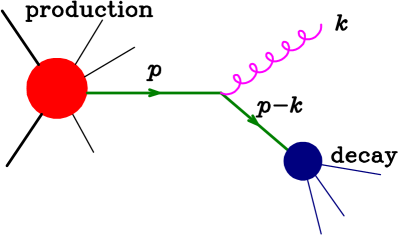
Figure 5: Insertion of a soft gluon in an internal resonance propagator.

we illustrate the insertion of a soft emission in an internal resonance line. The product of the resonance propagators will be given by

$$\frac{1}{p^{2}-M^{2}+i\Gamma M}\times\frac{1}{(p-k)^{2}-M^{2}+i\Gamma M}\\ =\frac{1}{2p\cdot k}\left[\frac{1}{(p-k)^{2}-M^{2}+i\Gamma M}-\frac{1}{p^{2}-M^{2}+i\Gamma M}\right].$$ (93)

Under the assumption that $\omega=k^{0}>\Gamma$, the two denominators cannot be near their mass shell at the same time. When the first term in the square bracket is near its mass shell, the process corresponds to the resonance radiating during production. In fact, in this case the $p$ momentum is far from the mass shell by a scale of order $k^{0}$, while the $p-k$ momentum is near the mass shell by a scale of order $\Gamma$. In coordinate space, this means that the line carrying momentum $p$ has a length of order $1/k^{0}$, much shorter than the length of order $1/\Gamma$ of the $p-k$ line. Conversely, if the second term is on-shell, radiation is taking place during decay. When squaring the amplitude, interference between these two terms is suppressed, since the two propagators cannot be on-shell at the same time, and the integration is effectively cut off by at a scale of order $\Gamma$, leaving no phase space for soft logarithms to build up. For the same reason, interference from emissions arising at production with emissions from resonance decay, as well as from emissions arising from the decay of different resonances, do not yield soft logarithms, since they also lead to propagators off the resonance peaks in the interfering amplitudes.

Reasoning in terms of radiation and decay times, by assuming $\omega>\Gamma_{0}$ we are assuming that radiation time is shorter than the resonances lifetimes. Thus, soft radiation in production cannot interfere with radiation in decays, since they happen at different times, and for the same reason radiation from different resonances cannot interfere. So, as far as soft singularities are concerned, the process can be though of as the product of independent production and decay processes, each one of them with resonances appearing only as initial or final state particles, but not as internal lines. For all these independent components, soft emissions is given by the usual eikonal formula applied only to initial and final state particles, that in this case can also be unstable resonances.

The structure of the soft singularity in region $b$ is determined by the initial and final state particles after the decay of all resonances. The resonances are considered as off-shell particles, as far as soft emissions are concerned, and interference terms from emissions arising from different resonances are not suppressed by small Breit-Wigner weights, since the emission energy is below the resonance widths. In terms of time, this is the case when the time for soft radiation is longer than the resonance widths, so that only particles that live longer than the resonances can contribute.

The form of the soft subtraction term in the $b$ region is the same one that we have adopted in the present method. However, that in our present treatment we are considering unrestricted emissions, while the $b$ region is defined to involve soft energies below $\Gamma_{0}$. When considering a given underlying Born resonance history, we will thus have the following cases:

• In the emissions from pairs of coloured massless partons belonging to the same resonance, the terms in regions $a$ and $b$ will combine, yielding an unrestricted soft energy integral, and no $\log\Gamma$ terms.

• In the emission from pairs of coloured massless partons belonging to different resonances, only the terms in the $b$ region will be present. These contributions will be cut-off at energies above $\Gamma_{0}$, since for larger energies they will push one of the two resonances out of its mass shell, thus damping the cross section. They will thus lead to $\log\Gamma$ contributions to the cross section.

• In any emission from an internal resonance leg, the emission energy will have a lower infrared cutoff $\Gamma_{0}$, and will yield other $\log\Gamma$ terms.

It is conceivable that our method may be modified, by adding further soft subtraction terms to the real cross section and corresponding integrated soft terms to the soft-virtual cross section, in such a way that the $\log\Gamma$ terms cancel within the soft-virtual contribution. This procedure may make the NLO calculation more convergent in the zero width limit. However, it would have no effect in the generation of radiation according to the POWHEG method. In POWHEG, the cancellation of the $\log\Gamma$ terms takes place numerically in the calculation of the $\tilde{B}$ function, between the real and the soft-virtual integral. In the generation of radiation, the cross section is unitarized by construction, so that no further $\log\Gamma$ terms arise in inclusive quantities. We thus did not attempt to implement such an improvement in the present work.

4 Code organization

The implementation of the subtraction scheme described in the present paper has required an extensive rewriting of several parts of the POWHEG BOX framework. While we postpone writing a full documentation for the new code, we will describe in the present section the structures that are used to describe the various components of the cross section in terms of flavour and resonance histories.

The flavour structures used to implement our subtraction scheme are organized as follows. The process specific code provides the flavour structure in terms of arrays carrying the flavour of the particles involved in the process, including intermediate resonances. We have the arrays

flst_born(1:flst_bornlength(iborn),iborn), iborn=1...flst_nborn;
flst_bornres(1:flst_bornlength(iborn),iborn), iborn=1...flst_nborn;

flst_real(1:flst_reallength(ireal),ireal), ireal=1...flst_nreal;
flst_realres(1:flst_reallength(ireal),ireal), ireal=1...flst_nreal.

These arrays are set in the user process routines. The following arrays are also set by the user process routines:

flst_bornresgroup(1:flst_nborn);
flst_nbornresgroup.

These have the purpose of grouping together the Born full flavour configurations that have similar resonance structure so that they can be integrated together. Thus, the value of flst_bornresgroup(iborn) (an integer from 1 to flst_nbornresgroup) labels the resonance structure group of the born full flavour structure iborn. This is needed because the POWHEG BOX groups together flavour structures with similar resonance histories when performing the integration, since these configuration can be integrated with the same importance sampling.

In the user process arrays, each flavour structure can appear only once, following the traditional approach of FNO. In the case of resonances, this leads to a non-trivial subtlety that we describe now. Consider the flavour structure for the subprocess $q\bar{q}\rightarrow e^{+}e^{-}e^{+}e^{-}$. According to the traditional approach of the POWHEG BOX there is only one flavour structure associated with this process, i.e. only a single ordering of the final state electron and positron will appear. When resonance structures are considered, we realize that we have two ways of pairing the electrons–anti-electrons to build an intermediate $Z$ boson. These two pairings are fully equivalent up to permutations of the final state particles, and thus only one resonance assignment will appear for them. We should not forget, however, that the contribution with a given resonance assignment carries a resonance projection factor. Assigning the ordering 1 to 8 to the $q\bar{q}\rightarrow ZZ\rightarrow e^{+}e^{-}e^{+}e^{-}$, assuming that the $Z$ in position 3 decays into the $e^{+}e^{-}$ pair in position 5-6, and assuming that we have only these two resonance histories, we will have a factor of the form

$$\frac{P(5,6;7,8)}{P(5,6;7,8)+P(5,8;7,6)},$$ (94)

where, for example,

$$P(5,6;7,8)=\frac{M_{Z}^{4}}{(s_{56}-M_{Z}^{2})^{2}+\Gamma_{Z}^{2}M_{Z}^{2}}\times\frac{M_{Z}^{4}}{(s_{78}-M_{Z}^{2})^{2}+\Gamma_{Z}^{2}M_{Z}^{2}}.$$ (95)

It is clear now that we should supply a factor of 2 for this graph, since by assigning the resonances we break part of the exchange symmetry for final state identical particles. Thus, the user process should provide the symmetry factor appropriate for the given final state irrespective of resonance assignment. The POWHEG machinery will take care of supplying the appropriate factors arising from the resonance assignment specification. Thus, the user process list is built from the list of flavour structures for all distinct final states (where distinct means that final state differing by permutations are not allowed). For each final state, the list will be expanded by assigning all possible resonance histories. But, again, full flavour structure differing only by a permutation of the resonance histories will not be allowed. The POWHEG BOX checks explicitly that no full flavour structures equivalent up to a permutation will appear.

Notice that the factor of two will lead to a total resonance factor of

$$\frac{2P(5,6;7,8)}{P(5,6;7,8)+P(5,8;7,6)},$$ (96)

that is not 1. However, by symmetry, an analysis of generated events that does not distinguish among identical final state particles will lead to the same results as if we included both weights

$$\frac{P(5,6;7,8)}{P(5,6;7,8)+P(5,8;7,6)}+\frac{P(5,8;7,6)}{P(5,6;7,8)+P(5,8;7,6)}=1.$$ (97)

Given the real, the POWHEG BOX finds all singular regions associated with the real graphs, and builds the corresponding arrays

flst_alr(1:flst_alrlength(alr),alr), alr=1...flst_nalr;
flst_alrres(1:flst_alrlength(alr),alr), alr=1...flst_nalr.

It furthermore fills the arrays flst_emitter(1:flst_nalr) with the emitter of the given singular region, and the array flst_alrmult(1:flst_nalr) with the multiplicity of the singular region. A multiplicity factor can arise if we have identical partons in the final state. For example, if we have several gluons and a quark in the final state, there will be regions associated with each gluon being collinear to the quark, and the program will find as many regions of this type as there are gluon. It will recognize that all these regions are equivalent, and it will emit a single region with a multiplicity factor equal to the number of equivalent regions.

If there are real contributions that do not have any singular region, they are collected into the ”regular” arrays

flst_regular(1:flst_regularlength(ireg),ireg), ire=1...flst_nregular;
flst_regularres(1:flst_regularlength(ireg),ireg), ireg=1...flst_nregular.

An array flst_regularmult(1:flst_nregular) is provided also in this case.

The task of finding out the singular and regular contributions is carried out by the subroutine genflavreglist, in the file find_regions.f. In the traditional POWHEG BOX implementation, at this stage, for each alr a list of competing singular regions was found. These were needed since each alr contribution is obtained by multiplying the corresponding real graph by the ratio of the $d^{-1}_{\alpha_{r}}$ factor divided by the sum of all the $d^{-1}_{\alpha_{r}}$ associated with the other competing singular regions. In the current implementation, we also need to list together the competing resonance histories that lead to the same final state, in order to compute the corresponding resonance projection factor. So, for either the alr, the regular or the Born terms, we have an array of pointers

flst_XXXnumrhptrs(1:flst_nXXX), flst_XXXrhptrs(maxreshists,flst_nXXX),

where XXX stands for either of alr, regular or born. The integer  flst_XXXnumrhptrs(iXXX) stores the number of resonance histories associated with the iXXX full flavour structure. The integers flst_XXXrhptrs(1:flst_XXXnumrhptrs(iXXX),iXXX), in case XXX is either alr or regular, are indices in the arrays

flst_allrhlength(maxreshists),
flst_allrh(nlegreal,maxreshists),
flst_allrhres(nlegreal,maxreshists),

that represent the full flavour structure of the competing resonance histories in the real graphs, and in case XXX is born, are indices in the arrays

flst_allbornrhlength(maxreshists),
flst_allbornrh(nlegborn,maxreshists),
flst_allbornrhres(nlegborn,maxreshists),

representing the full flavour structure of the competing resonance histories for the Born graphs. We stress that we cannot use flst_real and flst_born in place of flst_allrh and flst_allbornrh, because in the latter also configurations that differ by a permutation of the intermediate resonances are included. The rh arrays described above are filled by the subroutine fill_res_histories, in the fill_res_histories.f file, that also computes the multiplicity factor associated with alternative resonance histories that differ only by a permutation of the resonances from the contribution being considered. These arrays are required for the computation of the weights needed to project out a given resonance history contribution from the real and Born amplitudes. Besides these, in the case of the alr contributions, we also need to know the singular regions associated with a given resonance history. This information is contained in the arrays

flst_allrhnumreg(maxreshists),
flst_allrhreg(1:2,maxregions,maxreshists).

For each entry of the realrh arrays, flst_allrhnumreg gives the number of singular regions, and flst_allrhreg gives the indices of the two particles becoming collinear in the corresponding singular region.

5 The example of single top, $t$-channel production

We consider the Born level process $bq\rightarrow be^{+}\nu_{e}q^{\prime}$. In the following we will label for conciseness as $q$ and $q^{\prime}$ all light quarks or antiquarks (excluding the $b$) with the appropriate flavour structure that can appear in the process, and we imply also the presence of the corresponding processes with exchanged initial state particles (i.e. $qb$ in this case). This process is dominated by the single top production process $bq\rightarrow(t\rightarrow b(W^{+}\rightarrow e^{+}\nu_{e}))q^{\prime}$, such that the top quark is not produced at rest in the partonic centre-of-mass. Therefore this process is relevant for testing our formalism. In fact, the standard momentum mapping leading to the underlying Born configuration, in case of collinear radiation from the $b$ quark arising from top decay, would conserve the incoming partons 4-momentum by adjusting the 3-momenta of the $b$ and the $W^{+}q^{\prime}$ systems with appropriate boosts. This procedure would preserve the mass of the $W^{+}q^{\prime}$ system, but not the mass of the top.

At the Born level, it is enough to consider a single resonance history, namely $bq\rightarrow(t\rightarrow b(W^{+}\rightarrow e^{+}\nu_{e}))q^{\prime}$. Alternatively, one may consider two different resonance histories:

$$bq \rightarrow (t\rightarrow b(W^{+}\rightarrow e^{+}\nu_{e}))q^{\prime},$$ (98)

$$bq \rightarrow b(W^{+}\rightarrow e^{+}\nu_{e})q^{\prime}.$$ (99)

The second one is actually not needed, since treating the $bW^{+}$ system as a resonance (i.e. preserving its mass in the underling Born mapping) rather than preserving the mass of the $W^{+}q^{\prime}$ system, as the POWHEG BOX would do for the resonance history of eq. (99), does not lead to any inaccuracy. We did however include this resonance assignment as an option, and used it to test that our setup works also in the case when more than one resonance history is present at the Born level.

We are considering the following real processes: $bq\to e^{+}\nu_{e}q^{\prime}g$ and $bg\to e^{+}\nu_{e}qq^{\prime}$. We do not consider processes of the form $qg\to be^{+}\nu_{e}q^{\prime}\bar{b}$, that include also $s$-channel contributions. This is adequate for the purposes of the present paper, where we would like to present and validate a method, rather then provide a realistic simulation of single top production.

We will now list the resonance histories for the real contributions corresponding to the choice of a single resonance history at the Born level:

$$bq \rightarrow g(t\rightarrow b(W^{+}\rightarrow e^{+}\nu_{e}))q^{\prime},$$ (100)

$$bq \rightarrow (t\rightarrow bg(W^{+}\rightarrow e^{+}\nu_{e}))q^{\prime},$$ (101)

$$bg \rightarrow (t\rightarrow bg(W^{+}\rightarrow e^{+}\nu_{e}))qq^{\prime},$$ (102)

$$bg \rightarrow b(Z/\gamma\rightarrow(W^{+}\rightarrow e^{+}\nu_{e})(W^{-}\rightarrow qq^{\prime}))$$ (103)

$$bg \rightarrow (t\rightarrow bg(W^{+}\rightarrow e^{+}\nu_{e}))(W^{-}\rightarrow qq^{\prime})$$ (104)

Notice that the last two processes are really regular ones, since for them no collinear singularity can arise by pairing particles belonging to the same resonance.

The Born (together with the colour correlated Born) and real matrix elements for the process were easily generated using the MadGraph4-POWHEG interface described in ref. Campbell:2012am . The virtual contribution was extracted by hand from code generated using MadGraph5_aMC@NLO Alwall:2014hca .

5.1 Test at the NLO level

We first tested our method (that we refer to as POWHEG-BOX-RES) by comparing its NLO level results with a (traditional) POWHEG-BOX-V2 implementation of the same process. More specifically, we implemented the $bq\to be^{+}\nu+eq^{\prime}$ process in the POWHEG-BOX-V2 framework, without the inclusion of any resonance information, and using exactly the same matrix elements used with the new method. The comparison was carried out by using exactly the same choice of scales and parton density functions.

We observe that the process (103) has initial state collinear singularities, due to a contribution arising from an initial state $g\rightarrow b\bar{b}$ splitting followed by the subprocess $b\bar{b}\rightarrow(Z/\gamma\rightarrow(W^{+}\rightarrow e^{+}\nu_{e})(W^{-}\rightarrow qq^{\prime}))$. This process is not subtracted in our procedure, since we do not have a corresponding underlying Born contribution. In order to avoid the associated collinear divergence, and only in the framework of the NLO tests that we are discussing in this section, we supplied our cross section with a damping factor of the form

$$\frac{p_{t,b}^{2}}{p_{t,b}^{2}+20}\;,$$ (105)

that damps low transverse momentum $b$ emissions. It is applied to all terms of the cross section, as a function of the corresponding $b$ quark kinematics. We stress that this damping factor is not used when doing phenomenological calculations. It is needed here only to guarantee that the NLO cross sections computed with the traditional POWHEG BOX implementation is finite and agrees formally with the one computed with the new method.

In order to perform the NLO test we did not need the virtual contributions, since they are the same in the two approaches. In the ”traditional” implementation the Born phase space was generated with importance sampling on the dominant decay chain $bq\rightarrow(t\rightarrow b(W^{+}\rightarrow e^{+}\nu_{e}))q^{\prime}$. It was found that the new implementation yielded better convergence, speeding up the calculation by about a factor of 2 or more. Very high statistics runs of both implementations were performed, and full numerical agreement was found for both the total cross section and the differential distributions.

5.2 Results and comparisons at the full shower level

As mentioned earlier, the process we are considering is singular when final state $b$ quarks have very small transverse momenta. Thus, event generation requires a generation cut or a Born suppression factor Alioli:2010qp . We adopt the latter method in the present work, using a suppression factor of the form

$$\frac{p_{t,b}^{2}}{p_{t,b}^{2}+20}\;.$$ (106)

As a result, less and less events are generated as the $b$ transverse momentum becomes small, but the event weight is increased correspondingly, thus yielding a potentially divergent cross section for observables that do not suppress the contribution of small transverse momentum $b$ quarks.

The shower was performed using Pythia8 version 81.85 Sjostrand:2014zea ; Sjostrand:2007gs ; Sjostrand:2006za . In all cases, Pythia8 was run with its default initialization, supplemented with the following calls:

    pythia.readString("SpaceShower:pTmaxMatch = 1");
    pythia.readString("TimeShower:pTmaxMatch = 1");

    pythia.readString("SpaceShower:QEDshowerByQ = off"); // From quarks.
    pythia.readString("SpaceShower:QEDshowerByL = off"); // From Leptons.
    pythia.readString("TimeShower:QEDshowerByQ = off"); // From quarks.
    pythia.readString("TimeShower:QEDshowerByL = off"); // From Leptons.

    pythia.readString("PartonLevel:MPI = off");

The first two calls cause Pythia8 to veto emissions harder than scalup, if arising at production level, and to allow unrestricted emissions from resonance decays. Furthermore, $b$ hadron decays were switched off with calls of the following kind

  pythia.readString("521:mayDecay = off");
  pythia.readString("-521:mayDecay = off");

for all $b$ flavoured mesons and baryons.

In order to test our generator, we generated four samples of one million of events each, and compared the relative output. The samples are obtained as follows:

• NORES Sample. This is obtained using the traditional POWHEG-BOX-V2 implementation for the process. The events are fed to Pythia8, with the setting listed earlier. Pythia8 is required to veto radiations at scales harder than the value of the Les Houches variable scalup, set equal to the transverse momentum of the POWHEG generated radiation for each Les Houches event.

• RES-HR Sample. This sample is obtained using the POWHEG-BOX-RES implementation of the process. The Les Houches events include the hardest radiation generated by POWHEG (the HR in RES-HR stands for “hardest radiation”). Since POWHEG is generating the hardest radiation, besides vetoing radiation in production with the usual scalup mechanism, we also forbid any Pythia8 radiation from top decays harder than scalup. We do this by explicitly examining the showered events. If a radiation generated by Pythia8 in top decay has a transverse momentum greater than scalup, the program discards it, and runs Pythia8 again on the same Les Houches partonic event. This procedure is repeated indefinitely, thus explicitly vetoing any event with radiation harder than scalup.

• RES-AR Sample. This sample is obtained using the POWHEG-BOX-RES implementation of the process. However, rather than keeping only the hardest radiation, we kept both the hardest radiation in top decay and the hardest radiation in production (the AR in RES-AR stands for “all radiation”) . These radiations are composed into a single event, using the usual POWHEG mapping mechanism. In this case, besides the normal scalup veto for radiation in production, we must forbid Pythia8 radiation in top decays if harder than the POWHEG generated one in top decay. There are thus two different veto scales, one for production (i.e. the scalup value) and one for decay. There are no provisions in the Les Houches Interface for User Processes to store the radiation scale for decaying resonances. The program thus computes explicitly the transverse momentum of radiation in top decay at the Les Houches level. If the showered event contains shower generated radiation in top decay harder than this computed scale, the shower is discarded, and a new shower is generated on the same Les Houches event, repeating the procedure indefinitely until the event passes the required condition.

  The RES-AR implementation is fully analogous to the allrad procedure illustrated in ref. Campbell:2014kua . The method (and the software) for vetoing Pythia8 radiation is also borrowed from that reference.

• ST-tch Sample. This sample is generated using the ST-tch POWHEG generator of ref. Alioli:2009je . Radiation in decay is not included in this generator, and thus we let Pythia8 shower the event according to its default setup, vetoing events with radiation in production harder than scalup, and with no veto in top decays. In order to match more closely what we include in RES-HR, we deleted in the ST-tch the real processes initiated by a light (i.e. not $b$) quark and a gluon.

5.3 Phenomenological analysis

We have considered the LHC 8 TeV configuration for our phenomenological runs. We have used throughout the MSTW2008 set Martin:2009iq at NLO order. Other PDF sets, like those of refs. Lai:2010vv ; Ball:2010de , can be used as well, but we are not interested in a PDF comparison in the present study. We only consider the $b\,\mu^{+}\nu_{\mu}$ final state (i.e. not the conjugate one).

We set the top mass to $m_{t}=172.5$ GeV. For this value of the mass and PDF choice the computed top width, including NLO strong corrections, is $1.3306$ GeV. We use the same NLO value of the width also in the ST-tch generator. In this generator it only affects the top line-shape, since the cross section is determined by the top cross section multiplied by a user supplied branching fraction. On the other hand, in our generator the width must be computed with the same Standard Model parameters that are used in the matrix elements, since the cross section will be proportional to a partial width (depending upon the couplings that are used in the matrix elements) divided by the total width that appears in the denominator of the top propagator.

Since we will compare generators that do not include top resonance information, our analysis will be performed (unless explicitly stated otherwise) without using “Monte Carlo truth” information as far as the top particle is concerned, thus relying solely upon a particle level reconstruction of the top kinematics. We thus define the following objects:

• The lepton. This is the hardest $\mu^{+}$ in the event.

• The neutrino. This is the hardest $\nu_{\mu}$ in the event.

• The $W^{+}$. This is the system formed by the lepton and the neutrino.

• The $b$ hadron. This is the hardest hadron with a $b$ quark content (not a $\bar{b}$!).

• The $b$-jet. Jets are reconstructed using the anti-$k_{t}$ algorithm Cacciari:2008gp , as implemented in the FastJet package Cacciari:2011ma , with $R=0.5$. The $b$-jet is the jet that contains the $b$ hadron.

• The top quark. This is defined as the system comprising the $W$ and the $b$-jet. Only $b$-jets with a $p_{t}$ of at least 25 GeV and $|\eta|<4.5$ are accepted for this purpose. In case such a $b$-jet is not found, no top is reconstructed.

5.4 RES-AR and ST-tch comparison

We begin by comparing the RES-AR and the ST-tch results. For this purpose (and only in this case) we have deleted from the RES-AR generator the real amplitudes with the final non-$b$ light partons in a colour singlet. This excludes in particular contributions with $tW^{-}$ associated production, leading to a more meaningful comparison and to a better agreement on the total cross sections, since these contributions are not included in the ST-tch generator. In fig. 6

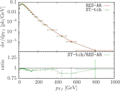
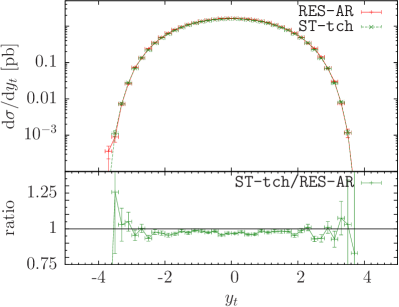
Figure 6: Transverse momentum distribution of the top quark, obtained with the RES-AR and the ST-tch generators.

we plot the transverse momentum and the rapidity distributions of the reconstructed top. In these plots no requirement is made on the mass of the reconstructed top. As one can see, reasonable agreement is found with these distributions. In fig. 7

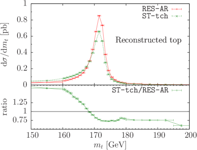
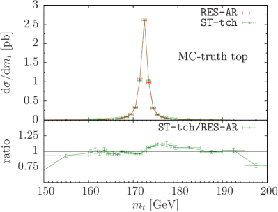
Figure 7: Invariant mass of the top quark, obtained with the RES-AR and the ST-tch generators, at the reconstructed level and at the MC-truth level.

we show the mass peak, both for the reconstructed top and for the top particle in the Monte Carlo record (more specifically, we pick the last top in the Monte Carlo event record). It is apparent that the line-shape of the reconstructed top are not in complete agreement. Assuming that this is due to differences in the structure of the $b$-jet, we plot in fig. 8

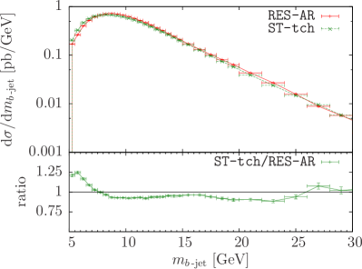
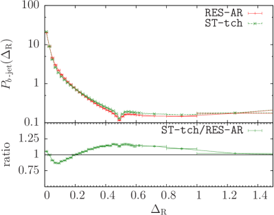
Figure 8: Mass and profile of the $b$ jet, obtained with the RES-AR and the ST-tch generators.

the $b$-jet mass and profile, for $b$-jets with transverse momentum above $15$ GeV and $|\eta|<4.5$. The jet profile is defined as follows

$$P_{b\operatorname{-jet}}(\Delta_{\mathrm{R}})=N\int{\mathrm{d}}\sigma\;\frac{\sum_{j}p_{T,j}\times\delta(\Delta_{\mathrm{R}}^{(j,b\operatorname{-jet})}-\Delta_{\mathrm{R}})}{p_{T,b\operatorname{-jet}}},$$ (107)

where $N$ is chosen in such a way that

$$\int_{0}^{0.5}P_{b\operatorname{-jet}}(\Delta_{\mathrm{R}})\mathrm{d}\Delta_{\mathrm{R}}=1\,,$$ (108)

where $0.5$ is the $\Delta_{\mathrm{R}}$ value that defines the $b$-jet. Thus, for $\Delta_{\mathrm{R}}<0.5$, $P_{b\operatorname{-jet}}(\Delta_{\mathrm{R}})$ is the fractional distribution of the transverse momentum in the jet. In fig. 9

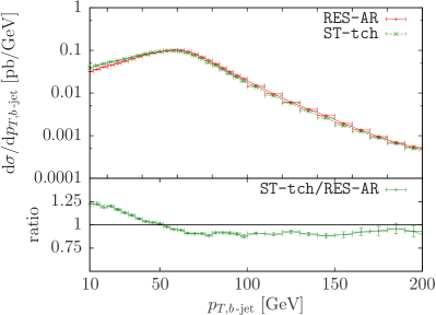
Figure 9: Transverse momentum of the $b$ jet, obtained with the RES-AR and the ST-tch generators.

we show the transverse momentum of the $b$-jet.

We see that these plots show consistently that the $b$-jet is harder and more massive in the RES-AR case than in the ST-tch one. In particular, the jet profile plot shows that there are more partons sharing the jet momentum in the region with $\Delta_{\rm R}$ near 0.1 in the RES-AR case. In the ST-tch case more momentum is concentrated at very small $\Delta_{R}$ (presumably due to the $b$ meson), and there are more partons at larger values of $\Delta_{R}$, also outside of the jet cone. We interpret these fact as consistent with the reconstructed top mass peak being slightly shifted to the right in the RES-AR case.

In order to quantify the shift in the mass extraction that one would get using one or the other Monte Carlo, we define an observable $M_{\rm trec}$, equal to the average value of the reconstructed top mass in a window of $\pm 15$ GeV around $m_{t}$, in order to mimic the typical experimental resolution on the reconstructed top mass. We get $M_{\rm trec}=170.54(2)$ GeV for the RES-AR, and $M_{\rm trec}=169.59(1)$ GeV for the ST-tch generator. Thus, extracting the top mass with the ST-tch generator we would get a value 1 GeV larger than if we used the RES-AR one.

As a further comment on our findings, we remind the reader that, as far as the reconstructed top line-shape is concerned, the RES-AR and ST-tch generators differ mainly in the way that radiation from the $b$ quark is treated. In the RES-AR generator the hardest radiation from the $b$ quark is always handled by POWHEG, with Pythia8 handling the remaining radiation. In the ST-tch generator, on the other hand, POWHEG generates no radiation from the decaying top. Thus, all radiation from the $b$ quark is handled by Pythia8. We must therefore ascribe the differences that we find to the different treatment of radiation in POWHEG and Pythia8. This issue was also discussed in ref. Campbell:2014kua . In view of its impact on the top mass determination, this topic deserves a more detailed phenomenological study, that goes beyond the scope of the present work.

5.5 RES-AR and RES-HR comparison

We now compare the RES-AR and RES-HR generators. As mentioned earlier, the two generators differ in the way that the Les Houches record is formed after the stage of generation of radiation. In the former, the hardest radiation is kept for both production and top decay independently. So, events with up to two more partons with respect to the Born kinematics are stored in the Les Houches record, and are passed to Pythia8 for showering. The shower in production is limited to the hardness of the radiation in production, while the shower in top decay is limited by the hardness of radiation in top decay. In the latter, only the hardest radiation of all is kept. Shower radiation, whether from production or from decay, is limited by the scale of the hardest radiation in POWHEG.

In fig. 10

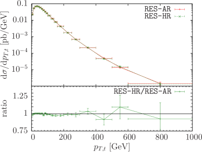
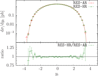
Figure 10: Transverse momentum distribution of the top quark, obtained with the RES-AR and the RES-HR generators.

we plot the transverse momentum and the rapidity distributions of the reconstructed top. In fig. 11

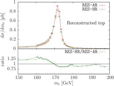
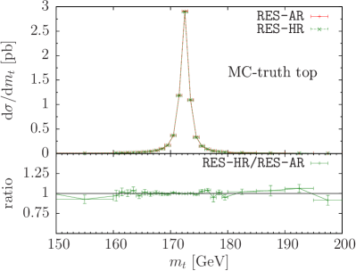
Figure 11: Invariant mass of the top quark, obtained with the RES-AR and the RES-HR generators, at the reconstructed level and at the MC-truth level.

we show the mass peak, both for the reconstructed top and for the top particle in the Monte Carlo record. In fig. 12

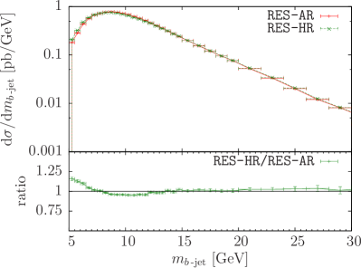
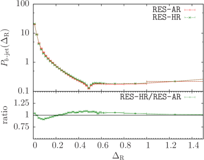
Figure 12: Mass and profile of the $b$-jet, obtained with the RES-AR and the RES-HR generators.

we plot the mass and profile of the $b$-jet, while in fig. 13

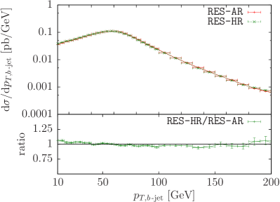
Figure 13: Transverse momentum of the $b$ jet, obtained with the RES-AR and the RES-HR generators.

we plot its transverse momentum.

We find, as in the case of the RES-AR and ST-tch comparison, differences in the top lineshape. In this case, however, they are less pronounced. The comparison of observables related to the $b$-jet also follow a similar pattern. They are qualitatively similar to the previous case, but less pronounced, in particular for the case of the $b$-jet transverse momentum distribution. We interpret these findings as being due to the fact that in the RES-HR generator the $b$-jet hardest radiation is in part controlled by POWHEG and in part by Pythia8. We remark that also in the RES-HR case POWHEG should correct the hardest radiation from the $b$ quark to yield an NLO accurate result, at least for sufficiently hard radiation.

It is again interesting to quantify the shift in the mass extraction that one would get using one or the other Monte Carlo. Computing, as before, our $M_{\rm trec}$ observable, we get $M_{\rm trec}=170.06(3)$ GeV for the RES-HR generator, and $M_{\rm trec}=170.55(2)$ GeV for the RES-AR. The small difference in the RES-AR result with respect to the one given in the previous subsection was due to the fact that there a set of real contributions was left out, as explained earlier.

5.6 NORES and RES-HR comparison

We now compare the NORES and RES-HR generators. The purpose of this comparison is to see if and how a generator that is not aware of resonance structures can exhibit visible distortions. In this case, MC resonance truth information is not available for the NORES generator. It is possible however to try to guess the resonance information from the structure of the event, as we will detail later.

We begin by showing results with the NORES contribution without performing any resonance assignment. In fig. 14

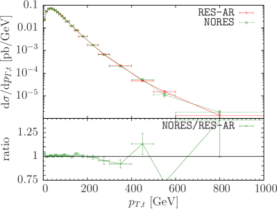
Figure 14: Transverse momentum distribution of the top quark, obtained with the NORES and the RES-HR generators.

we plot the transverse momentum and the rapidity distributions of the reconstructed top. In fig. 15

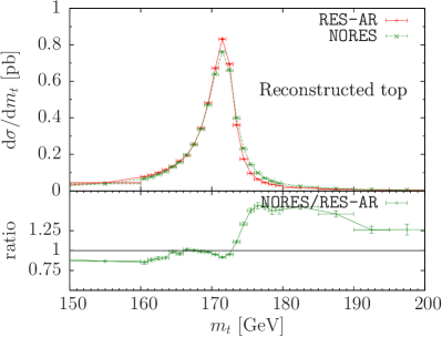
Figure 15: Invariant mass of the top quark, obtained with the NORES and the RES-HR generators, at the reconstructed level.

we show the mass peak for the reconstructed top. In fig. 16

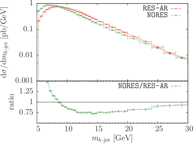
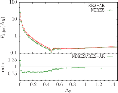
Figure 16: Mass and profile of the $b$ jet, obtained with the NORES and the RES-HR generators.

we plot the $b$-jet mass and profile. In fig. 17

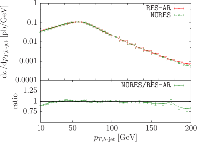
Figure 17: Transverse momentum of the $b$ jet, obtained with the NORES and the RES-HR generators.

we show the $b$-jet transverse momentum.

We see marked distortions in the mass peak, in the $b$-jet mass and profile, and in the transverse momentum distribution. In this case we get $M_{\rm trec}=170.54(2)$ GeV for the NORES and $M_{\rm trec}=170.06(3)$ GeV for the RES-HR generator. We remark that in this case no MC-truth was available for the top quark mass in the NORES case, and thus the corresponding plot is missing.

Finally, we performed a guess resonance assignment on the NORES output record, in the following way:

• The $b\,\mu^{+}\nu_{\mu}$ system is assigned to the top in all events.

• If the radiated parton is a gluon, and the $g\,b$ system has the colour of a quark, then we compute the transverse momentum of the gluon relative to the beam axis, $k_{T,{\rm isr}}$, relative to the final state light quark, $k_{T,{\rm fsr}}$, and relative to the $b$ quark in the $g\,b\,\mu^{+}\nu_{\mu}$ frame, $k_{T,b}$. Furthermore we compute the quantities

  $$f_{1} = \frac{1}{(s_{b\,\mu^{+}\nu_{\mu}}-m_{t}^{2})^{2}+(\Gamma_{t}m_{t})^{2}}\,,$$ (109)

  $$f_{2} = \frac{1}{(s_{g\,b\,\mu^{+}\nu_{\mu}}-m_{t}^{2})^{2}+(\Gamma_{t}m_{t})^{2}}\,.$$ (110)

  The gluon is assigned or not assigned to the top resonance with probabilities proportional to

  $$\frac{f_{2}}{k_{T,b}^{2}}\quad{\rm and}\quad f_{1}\times\left(\frac{1}{k_{T,{\rm isr}}^{2}}+\frac{1}{k_{T,{\rm fsr}}^{2}}\right)\,.$$ (111)

• If the radiated parton is not a gluon, it is not assigned to the top.

We label as NORES-i (i for “improved”) the corresponding generator, and show its comparison with the RES-HR output in figs. 18 through 21.

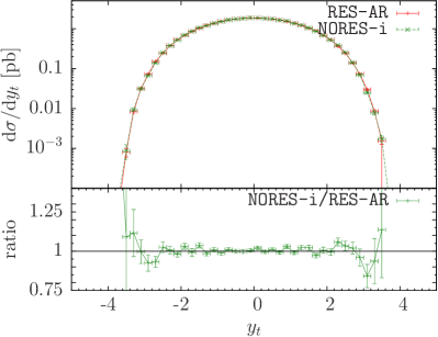
Figure 18: Transverse momentum distribution of the top quark, obtained with the NORES-i and the RES-HR generators.

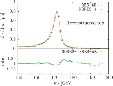
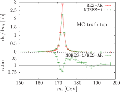
Figure 19: Invariant mass of the top quark, obtained with the NORES-i and the RES-HR generators, both at the reconstructed and at the MC-truth level.

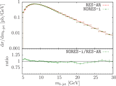
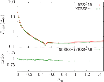
Figure 20: Mass and profile of the $b$ jet, obtained with the NORES-i and the RES-HR generators.

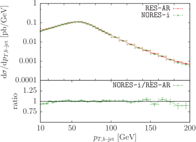
Figure 21: Transverse momentum of the $b$ jet, obtained with the NORES-i and the RES-HR generators.

We see that now the differences are much less pronounced, and do not seem to affect significantly the determination of the top mass. In fact, the average value of our $M_{\rm trec}$ observable is now $M_{\rm trec}=170.07(2)$ GeV for the NORES-i and $M_{\rm trec}=170.06(3)$ GeV for the RES-HR generator. Mild distortions are observed for the remaining distributions. On the other hand, we see that the MC-truth top line-shape seems to exhibit unphysical features, presumably due to the way that resonance assignment was performed.

6 Conclusions

In this work we have presented a formalism for dealing with intermediate resonances in NLO+PS generators built within the POWHEG framework. We have formulated a subtraction method such that no double logarithms of the resonance’s width arise separately in the integrated real and in the soft-virtual term of the NLO calculation. Single logarithms of the widths do however arise in the soft-virtual term (in fact in the virtual contribution) and in the integrated real cross section, and cancel only when adding them up. Thus, in the framework of a POWHEG generator, these single log terms cancel in the $\tilde{B}$ function, so that both double and single logarithms of the resonance widths are absent there. In POWHEG, the generation of radiation is unitarized by construction. Therefore, all soft divergences (including also those that are cut-off by the resonance width) are properly regulated there by Sudakov form factors and/or by finite width effects.

Our formalism is fully general, and has been implemented in a general way in a modified version of the POWHEG-BOX-V2. The framework is such that in order to implement a specific process, one must supply the Born, including spin and colour correlated amplitudes, the virtual and the real amplitudes. The framework takes care of everything else: it finds the possible resonance histories and singular regions, it builds a Born phase space consistent with the resonance histories, and it constructs the subtraction terms, the soft-virtual contributions and the mismatch terms described in sec. 3. It then performs the various stages of the POWHEG event generation.

In the present work we have considered, as a test case, the process $pp\to\mu^{+}\nu_{\mu}j_{b}j$, that is dominated by single-top $t$-channel production, in the 5-flavours scheme. Within this framework, we have examined the output of our generator, with particular attention to observables that can have an impact on the top mass measurements.

We have compared two variants of our generators. In the first one we use the traditional POWHEG method, dubbed RES-HR in this paper, retaining only the hardest radiation, feeding the corresponding partonic event to a shower Monte Carlo, and vetoing any shower-generated radiation harder than the POWHEG one. In the second one, dubbed RES-AR, the hardest radiations in production and in resonance decays are both kept and combined in the final partonic event. In this case, the veto scales on the hardness of the Shower radiation in production and in decays are different, being set to the corresponding scales of radiation in POWHEG. We also compare our generator to the previous single-top, t-channel generator, the ST-tch process of ref. Alioli:2009je in the POWHEG-BOX-V2. We can briefly summarize our findings as follows. We find differences in the reconstructed top, mostly due to the structure of the $b$-jets, and we ascribe these differences to the fact that the hardest radiation in the $b$-jet is fully determined by the Shower Monte Carlo in the ST-tch generator, it is in part determined by POWHEG and in part by the Shower Monte Carlo in the RES-HR generator, and it is fully determined by POWHEG in the RES-AR generator.

We have also considered the output of a generator using the same, full matrix elements for the $pp\to\mu^{+}\nu_{\mu}j_{b}j$ process that we have used in our new generator, implemented however in the traditional POWHEG-BOX-V2 framework, that is to say without resonance aware formalism. In this context we have again considered two alternative options. In the first one we pass the events to the Shower Monte Carlo without any resonance information. In the second one we reconstruct a most probable resonance history of the event based upon kinematics. The aim of such test is to search for distortions in the generated radiation due to the lack of proper treatment of resonance decays. We have found that if no resonance information is passed to the shower important differences are in fact observed. On the other hand, if we make an educated guess of the event resonance history, and pass it to the shower, smaller differences are present at the reconstructed level, although the top line-shape at the MC-truth level exhibits unphysical features.

We remark that one comparison is still missing in the present work: the comparison to a generator using the on-shell approximation (i.e. a single top generator analogous to the ttb_NLO_dec $t\bar{t}$ generator of ref. Campbell:2014kua ), in order to check if off-shell and non-resonant contributions at the radiation level are relevant for an accurate simulation of the production of a top resonance.

The relevant code for the present work is available in the POWHEG BOX repository at the url http://powhegbox.mib.infn.it/POWHEG-BOX-RES-beta. It has to be considered as very preliminary at the present stage, since only one relatively simple process has been implemented with it so far.

References

- (1) G. Altarelli, R. K. Ellis, and G. Martinelli, Large Perturbative Corrections to the Drell-Yan Process in QCD, Nucl.Phys. B157 (1979) 461.
- (2) R. K. Ellis, D. Ross, and A. Terrano, The Perturbative Calculation of Jet Structure in e+ e- Annihilation, Nucl.Phys. B178 (1981) 421.
- (3) Z. Kunszt, P. Nason, G. Marchesini, and B. Webber, QCD AT LEP, Proceedings of physics at LEP 1, vol. 1, 373–453, Geneva 1989.
- (4) B. Mele, P. Nason, and G. Ridolfi, QCD radiative corrections to Z boson pair production in hadronic collisions, Nucl.Phys. B357 (1991) 409–438.
- (5) M. L. Mangano, P. Nason, and G. Ridolfi, Heavy quark correlations in hadron collisions at next-to-leading order, Nucl.Phys. B373 (1992) 295–345.
- (6) S. Catani and M. Seymour, A General algorithm for calculating jet cross-sections in NLO QCD, Nucl.Phys. B485 (1997) 291–419, [hep-ph/9605323].
- (7) S. Frixione, Z. Kunszt, and A. Signer, Three jet cross-sections to next-to-leading order, Nucl.Phys. B467 (1996) 399–442, [hep-ph/9512328].
- (8) K. Melnikov, A. Scharf, and M. Schulze, Top quark pair production in association with a jet: QCD corrections and jet radiation in top quark decays, Phys.Rev. D85 (2012) 054002, [arXiv:1111.4991].
- (9) J. M. Campbell and R. K. Ellis, Top-quark processes at NLO in production and decay, J.Phys. G42 (2015), no. 1 015005, [arXiv:1204.1513].
- (10) S. Frixione and B. R. Webber, Matching NLO QCD computations and parton shower simulations, JHEP 0206 (2002) 029, [hep-ph/0204244].
- (11) P. Nason, A New method for combining NLO QCD with shower Monte Carlo algorithms, JHEP 0411 (2004) 040, [hep-ph/0409146].
- (12) S. Frixione, P. Nason, and C. Oleari, Matching NLO QCD computations with Parton Shower simulations: the POWHEG method, JHEP 0711 (2007) 070, [arXiv:0709.2092].
- (13) S. Alioli, P. Nason, C. Oleari, and E. Re, A general framework for implementing NLO calculations in shower Monte Carlo programs: the POWHEG BOX, JHEP 1006 (2010) 043, [arXiv:1002.2581].
- (14) J. M. Campbell, R. K. Ellis, P. Nason, and E. Re, Top-pair production and decay at NLO matched with parton showers, JHEP 04 (2015) 114, [arXiv:1412.1828].
- (15) P. Nason, MINT: A Computer program for adaptive Monte Carlo integration and generation of unweighted distributions, arXiv:0709.2085.
- (16) J. M. Campbell, R. K. Ellis, R. Frederix, P. Nason, C. Oleari, et al., NLO Higgs Boson Production Plus One and Two Jets Using the POWHEG BOX, MadGraph4 and MCFM, JHEP 1207 (2012) 092, [arXiv:1202.5475].
- (17) J. Alwall, R. Frederix, S. Frixione, V. Hirschi, F. Maltoni, et al., The automated computation of tree-level and next-to-leading order differential cross sections, and their matching to parton shower simulations, JHEP 1407 (2014) 079, [arXiv:1405.0301].
- (18) S. Alioli, P. Nason, C. Oleari, and E. Re, Vector boson plus one jet production in POWHEG, JHEP 1101 (2011) 095, [arXiv:1009.5594].
- (19) T. Sjöstrand, S. Ask, J. R. Christiansen, R. Corke, N. Desai, P. Ilten, S. Mrenna, S. Prestel, C. O. Rasmussen, and P. Z. Skands, An Introduction to PYTHIA 8.2, Comput. Phys. Commun. 191 (2015) 159–177, [arXiv:1410.3012].
- (20) T. Sjostrand, S. Mrenna, and P. Z. Skands, A Brief Introduction to PYTHIA 8.1, Comput. Phys. Commun. 178 (2008) 852–867, [arXiv:0710.3820].
- (21) T. Sjostrand, S. Mrenna, and P. Z. Skands, PYTHIA 6.4 Physics and Manual, JHEP 05 (2006) 026, [hep-ph/0603175].
- (22) S. Alioli, P. Nason, C. Oleari, and E. Re, NLO single-top production matched with shower in POWHEG: s- and t-channel contributions, JHEP 09 (2009) 111, [arXiv:0907.4076]. [Erratum: JHEP02,011(2010)].
- (23) A. Martin, W. Stirling, R. Thorne, and G. Watt, Parton distributions for the LHC, Eur.Phys.J. C63 (2009) 189–285, [arXiv:0901.0002].
- (24) H.-L. Lai, M. Guzzi, J. Huston, Z. Li, P. M. Nadolsky, et al., New parton distributions for collider physics, Phys.Rev. D82 (2010) 074024, [arXiv:1007.2241].
- (25) R. D. Ball, L. Del Debbio, S. Forte, A. Guffanti, J. I. Latorre, et al., A first unbiased global NLO determination of parton distributions and their uncertainties, Nucl.Phys. B838 (2010) 136–206, [arXiv:1002.4407].
- (26) M. Cacciari, G. P. Salam, and G. Soyez, The Anti-k(t) jet clustering algorithm, JHEP 0804 (2008) 063, [arXiv:0802.1189].
- (27) M. Cacciari, G. P. Salam, and G. Soyez, FastJet User Manual, Eur.Phys.J. C72 (2012) 1896, [arXiv:1111.6097].