Message-Passing Receiver for Joint Channel Estimation and Decoding in 3D Massive MIMO-OFDM Systems

Sheng Wu, , Linling Kuang, ,
Zuyao Ni, Defeng (David) Huang, ,
Qinghua Guo, , and Jianhua Lu
This work was partially supported by the National Nature Science Foundation of China (Grant Nos. 91338101, 61231011, and 91438206), the National Basic Research Program of China (Grant No. 2013CB329001), and Tsinghua University Initiative Scientific Research Program (Grant No. 20131089219). Sheng Wu, Linling Kuang and Zuyao Ni are with the Tsinghua Space Center, Tsinghua University, China (e-mail: {thuraya, kll, nzy}@tsinghua.edu.cn). Defeng (David) Huang is with the School of Electrical, Electronic and Computer Engineering, The University of Western Australia, Australia (e-mail: david.huang@ee.uwa.edu.au). Q. Guo is with the School of Electrical, Computer and Telecommunications Engineering, University of Wollongong, Australia, and is also with the School of Electrical, Electronic and Computer Engineering, The University of Western Australia, Australia (e-mail: qinghua.guo@uow.edu.au). Jianhua Lu is with the Department of Electronic Engineering, Tsinghua University, China (e-mail: lhh-dee@mail.tsinghua.edu.cn).
Abstract

In this paper, we address the message-passing receiver design for the 3D massive MIMO-OFDM systems. With the aid of the central limit argument and Taylor-series approximation, a computationally efficient receiver that performs joint channel estimation and decoding is devised by the framework of expectation propagation. Specially, the local belief defined at the channel transition function is expanded up to the second order with Wirtinger calculus, to transform the messages sent by the channel transition function to a tractable form. As a result, the channel impulse response (CIR) between each pair of antennas is estimated by Gaussian message passing. In addition, a variational expectation-maximization (EM)-based method is derived to learn the channel power-delay-profile (PDP). The proposed joint algorithm is assessed in 3D massive MIMO systems with spatially correlated channels, and the empirical results corroborate its superiority in terms of performance and complexity.

Index Terms:
Expectation Propagation, Joint Channel Estimation and Decoding, 3D Massive MIMO, Message Passing, OFDM.

I Introduction

Recently, massive multiple-input multiple-output (MIMO) systems with tens to hundreds of antennas at the base-station (BS) have gained significant attention [1, 2, 3, 4]. It has been proved that massive MIMO systems can scale down transmit power as well as increase spectrum efficiency by orders of magnitude [2]. One of the tasks in massive MIMO systems is estimating the channel impulse response (CIR) for each transmit-receive link, since high data rates and energy efficiency can only be achieved when CIR is known [5]. In contrast to the conventional MIMO systems employing a small number of antennas, there are a large number of channels need to be estimated. The pilot overhead required for channel estimation is proportional to the number of transmit antennas, which can be excessive in massive MIMO systems [6]. In the meantime, the available resources for training are restricted by the channel coherence time. On the other hand, the energy consumption by baseband processing grows with the number of antennas, which may obliterate the advantage of massive MIMO systems in energy efficiency. Thus, low-complexity channel estimation with high accuracy and reduced overhead is critical to massive MIMO systems.

Iterative receivers that jointly estimate the channel coefficients and detect the data symbols are able to provide more accurate channel estimation with less training overhead [7, 8, 9, 10, 11, 12]. Factor graph and sum-product algorithm (SPA) [13] have been used as a unified framework for iterative joint data detection, channel estimation, interference cancellation, and decoding [14, 15]. However, exact SPA for joint channel estimation and decoding is computationally infeasible. To overcome this problem, various message-passing algorithms based on approximate inference have been proposed [16, 17, 18, 19, 20, 21, 8, 22, 23]. In existing approaches, the message passing strategies include loopy belief propagation (LBP) [16, 19, 20, 21, 8], variational methods [24, 17, 23], and a hybrid of both [18, 22].

LBP has a high complexity when applied to graphical models that involve both discrete and continuous random variables. This has been addressed by merging the SPA with the expectation-maximization (EM) algorithm [19] or approximating the messages of SPA with Gaussian messages [25, 20, 19, 8]. Variational inference methods have been applied to MIMO receivers for joint detection, channel estimation, and decoding [17]. In [18], Riegler et al. derived a generic message-passing algorithm that merges belief propagation (BP) with the mean-field (MF) approximation (BP-MF), and applied it to joint channel estimation and decoding in single-input single-output orthogonal frequency division multiplex (OFDM) systems and MIMO-OFDM systems [18, 26, 22]. The BP-MF has to learn the noise precision to take into account the residual interference from other users even when the noise power is known [27, 28], as the channel transition functions are incorporated into the MF part [18, 26, 22]. Otherwise, the uncertainty of residual interference is completely ignored, and the likelihood function associated with the messages extracted from observations tends to overwhelm the a priori probability. Besides, the BP-MF requires high computational complexity as large matrices need to be inverted to estimate channel frequency response (CFR) [18], and thereby it is only feasible in the case of a few antennas and subcarriers. We note that there is a low-complexity version of the BP-MF algorithm proposed in [29], but its performance is inferior. The degraded performance may be due to the unrealistic assumption that groups of contiguous channel weights in frequency-domain obey a Markov model.

To achieve joint channel estimation and decoding for massive MIMO systems using OFDM modulation in frequency-selective channels, the receiver needs to complete three tasks: decoupling frequency-domain channel coefficients and data symbols from noisy observations, decoding, and channel estimation. Via central-limit theorem and moment matching, an approximate BP has been derived in [8], [16] and [21]. Despite its superior performance, the approximate BP bears a heavy computation burden: it needs to take a large number of moment-matching operations, each being highly complicated. In this paper, we use the framework of expectation propagation (EP) [30] to derive an efficient message-passing algorithm. Specifically, at the channel transition functions, we use the central-limit theorem to efficiently obtain the beliefs of frequency-domain channel coefficients and the beliefs of data symbols, and then employ a quadratic approximation to project them into the Gaussian family. In the meantime, the expectation propagation principle is applied to the symbol-variable nodes. As the beliefs of frequency-domain channel coefficients are now in the form of Gaussian family, a Gaussian message passing based estimator [31] can be employed, which exploits the fact that the CFR is the Fourier transformation of the CIR. Furthermore, using the beliefs of time-domain channel taps, the unknown power-delay-profile (PDP) can be learned by variational expectation maximization. We note that Parker et al. applied central-limit theorem and Taylor-series approximations to formulate a bilinear generalized approximate message-passing algorithm for the SPA in the high dimensional limit [32], but its scope is different from that of this work.

The proposed scheme of joint channel estimation and decoding is assessed in 3D massive MIMO systems with spatially correlated channels. Experiments show that its performance is within 1 dB of the known-channel bound in both a 64×864864\times 8 MIMO system and a 16×816816\times 8 MIMO system, and outperforms the performance of BP-MF by 0.4 dB in the 16×816816\times 8 MIMO system, the low-complexity version of BP-MF by 1.2 dB in the 64×864864\times 8 MIMO system and 1.6 dB in the 16×816816\times 8 MIMO system. On the other hand, the complexity of the proposed algorithm is a small percentage of that of BP-MF and 1313\frac{1}{3} of that of the low-complexity version of BP-MF.

The remainder of this paper is organized as follows. The system model is described in Section II. In Section III the message passing for joint detection and decoding is detailed. Complexity comparisons are shown in Section IV, and numerical results are provided in Section V, followed by conclusions in Section VI.

Notation: Lowercase letters (e.g., x𝑥x) denote scalars, bold lowercase letters (e.g.,𝒙𝒙\boldsymbol{x}) denote column vectors, and bold uppercase letters (e.g., 𝑿𝑿\boldsymbol{X}) denote matrices. The superscripts ()𝖳superscript𝖳(\cdot)^{\mathsf{T}}, ()𝖧superscript𝖧(\cdot)^{\mathsf{H}} and ()superscript(\cdot)^{*} denote the transpose operation, Hermitian transpose operation, and complex conjugate operation, respectively. Also, 𝖽𝗂𝖺𝗀{𝒙}𝖽𝗂𝖺𝗀𝒙\mathsf{diag}\{\boldsymbol{x}\} denotes a square diagonal matrix with the elements of vector 𝒙𝒙\boldsymbol{x} on the main diagonal; 𝑿𝒀tensor-product𝑿𝒀\boldsymbol{X}\otimes\boldsymbol{Y} denotes Kronecker product of 𝑿𝑿\boldsymbol{X} and 𝒀𝒀\boldsymbol{Y}; 𝑰𝑰\boldsymbol{I} denotes an identity matrix; and 𝗅𝗇()𝗅𝗇\mathsf{ln}(\cdot) denotes the natural logarithm. Furthermore, 𝒩(x;x^,νx)=(πνx)1exp(|xx^|2/νx)subscript𝒩𝑥^𝑥subscript𝜈𝑥superscript𝜋subscript𝜈𝑥1superscript𝑥^𝑥2subscript𝜈𝑥\mathcal{N}_{\mathbb{C}}(x;\hat{x},\nu_{x})=(\pi\nu_{x})^{-1}\exp(-\left|x-\hat{x}\right|^{2}/\nu_{x}) denotes the Gaussian probability density function (PDF) of x𝑥x with mean x^^𝑥\hat{x} and variance νxsubscript𝜈𝑥\nu_{x}; and 𝖦𝖺𝗆(γ;α,β)=βαγα1exp(βγ)/Γ(α)𝖦𝖺𝗆𝛾𝛼𝛽superscript𝛽𝛼superscript𝛾𝛼1𝛽𝛾Γ𝛼\mathsf{Gam}(\gamma;\alpha,\beta)=\beta^{\alpha}\gamma^{\alpha-1}\exp(-\beta\gamma)/\Gamma(\alpha) denotes the Gamma PDF of γ𝛾\gamma with shape parameter α𝛼\alpha and rate parameter β𝛽\beta, where Γ()Γ\Gamma(\cdot) is the gamma function. Finally, proportional-to\propto denotes equality up to a constant scale factor; 𝒙\xtnk\𝒙subscript𝑥𝑡𝑛𝑘\boldsymbol{x}\backslash x_{tnk} denotes all elements in 𝒙𝒙\boldsymbol{x} but xtnksubscript𝑥𝑡𝑛𝑘x_{tnk}; and 𝖤p(x){}subscript𝖤𝑝𝑥\mathsf{E}_{p(x)}\{\cdot\} denotes expectation with respect to distribution p(x)𝑝𝑥p(x).

II System Model

We consider the uplink of a massive MIMO system where N𝑁N single antenna users communicate with a BS simultaneously. The BS employs a uniform planar array (UPA) consisting of M=(D×W)N𝑀𝐷𝑊much-greater-than𝑁M=(D\times W)\gg N antennas distributed across D𝐷D rows and W𝑊W columns. Frequency-selective block-fading channels are assumed, and OFDM is employed to combat multipath interference.

II-A Channel Model

The CIR between the nth𝑛thn\text{th} user and the mth𝑚thm\text{th} receive antenna is denoted by 𝒉mn=[hmn1hmnL]𝖳subscript𝒉𝑚𝑛superscriptdelimited-[]subscript𝑚𝑛1subscript𝑚𝑛𝐿𝖳\boldsymbol{h}_{mn\cdot}=[h_{mn1}\cdots h_{mnL}]^{\mathsf{T}}, where hmnlsubscript𝑚𝑛𝑙h_{mnl} is the lth𝑙thl\text{th} path gain and L𝐿L is the maximum channel spread. Let 𝒉nl=[h1nlhMnl]𝖳subscript𝒉absent𝑛𝑙superscriptdelimited-[]subscript1𝑛𝑙subscript𝑀𝑛𝑙𝖳\boldsymbol{h}_{\cdot nl}=[h_{1nl}\cdots h_{Mnl}]^{\mathsf{T}} denote gain vector of the lth𝑙thl\text{th} paths between user n𝑛n and all the M𝑀M receive antennas at the BS. Due to close antenna spacing at the BS, we can assume that the M𝑀M CIRs between the user n𝑛n and all the M𝑀M receive antennas at the BS follow an identical PDP {𝖤{|hmnl|2}αnl,m}𝖤superscriptsubscript𝑚𝑛𝑙2subscript𝛼𝑛𝑙for-all𝑚\{\mathsf{E}\{|h_{mnl}|^{2}\}\triangleq\alpha_{nl},\forall m\}. We can also assume that the transmit antennas from different users are spatially uncorrelated. Accordingly, the Kronecker spatial fading correlation model for the gain vector 𝒉nlsubscript𝒉absent𝑛𝑙\boldsymbol{h}_{\cdot nl} is given by [33]

𝒉nl=𝑹nl12𝒉nl𝗂𝗂𝖽,subscript𝒉absent𝑛𝑙superscriptsubscript𝑹𝑛𝑙12superscriptsubscript𝒉𝑛𝑙𝗂𝗂𝖽\boldsymbol{h}_{\cdot nl}=\boldsymbol{R}_{nl}^{\frac{1}{2}}\boldsymbol{h}_{nl}^{\mathsf{iid}}, (1)

where 𝑹nlM×Msubscript𝑹𝑛𝑙superscript𝑀𝑀\boldsymbol{R}_{nl}\in\mathbb{C}^{M\times M} denotes the receive correlation matrix, and 𝒉nl𝗂𝗂𝖽M×1superscriptsubscript𝒉𝑛𝑙𝗂𝗂𝖽superscript𝑀1\boldsymbol{h}_{nl}^{\mathsf{iid}}\in\mathbb{C}^{M\times 1} denotes independent complex Gaussian matrix with zero mean and covariance matrix αnl𝑰subscript𝛼𝑛𝑙𝑰\alpha_{nl}\boldsymbol{I}. A ray-based 3D channel model from [34] is employed, and the receive correlation matrix 𝑹nlsubscript𝑹𝑛𝑙\boldsymbol{R}_{nl} is approximated by

𝑹nl𝑹nl𝖺𝗓𝑹nl𝖾𝗅,subscript𝑹𝑛𝑙tensor-productsuperscriptsubscript𝑹𝑛𝑙𝖺𝗓superscriptsubscript𝑹𝑛𝑙𝖾𝗅\boldsymbol{R}_{nl}\approx\boldsymbol{R}_{nl}^{\mathsf{az}}\otimes\boldsymbol{R}_{nl}^{\mathsf{el}}, (2)

where 𝑹nl𝖺𝗓W×Wsuperscriptsubscript𝑹𝑛𝑙𝖺𝗓superscript𝑊𝑊\boldsymbol{R}_{nl}^{\mathsf{az}}\in\mathbb{R}^{W\times W} and 𝑹nl𝖾𝗅D×Dsuperscriptsubscript𝑹𝑛𝑙𝖾𝗅superscript𝐷𝐷\boldsymbol{R}_{nl}^{\mathsf{el}}\in\mathbb{R}^{D\times D} are the correlation matrices in azimuth and elevation directions, respectively, and are defined by [34]

[𝑹nl𝖺𝗓]wwsubscriptdelimited-[]superscriptsubscript𝑹𝑛𝑙𝖺𝗓𝑤superscript𝑤\displaystyle[\boldsymbol{R}_{nl}^{\mathsf{az}}]_{ww^{\prime}} =1b𝖾𝗑𝗉(a2𝖼𝗈𝗌2(θnl𝖺𝗓)2jc𝖼𝗈𝗌(θnl𝖺𝗓)+νnl𝖺𝗓(c𝗌𝗂𝗇(θnl𝖺𝗓))22b),absent1𝑏𝖾𝗑𝗉superscript𝑎2superscript𝖼𝗈𝗌2superscriptsubscript𝜃𝑛𝑙𝖺𝗓2𝑗𝑐𝖼𝗈𝗌superscriptsubscript𝜃𝑛𝑙𝖺𝗓superscriptsubscript𝜈𝑛𝑙𝖺𝗓superscript𝑐𝗌𝗂𝗇superscriptsubscript𝜃𝑛𝑙𝖺𝗓22𝑏\displaystyle=\frac{1}{\sqrt{b}}\mathsf{exp}\left(-\frac{a^{2}\mathsf{cos}^{2}(\theta_{nl}^{\mathsf{az}})-2jc\mathsf{cos}(\theta_{nl}^{\mathsf{az}})+\nu_{nl}^{\mathsf{az}}\left(c\mathsf{sin}(\theta_{nl}^{\mathsf{az}})\right)^{2}}{2b}\right), (3)
[𝑹nl𝖾𝗅]ddsubscriptdelimited-[]superscriptsubscript𝑹𝑛𝑙𝖾𝗅𝑑superscript𝑑\displaystyle{}[\boldsymbol{R}_{nl}^{\mathsf{el}}]_{dd^{\prime}} =𝖾𝗑𝗉(2jπλd𝖾𝗅(dd)𝖼𝗈𝗌(θnl𝖾𝗅)νnl𝖾𝗅(πd𝖾𝗅(dd)𝗌𝗂𝗇(θnl𝖾𝗅))2λ2),absent𝖾𝗑𝗉2𝑗𝜋𝜆superscript𝑑𝖾𝗅superscript𝑑𝑑𝖼𝗈𝗌superscriptsubscript𝜃𝑛𝑙𝖾𝗅superscriptsubscript𝜈𝑛𝑙𝖾𝗅superscript𝜋superscript𝑑𝖾𝗅superscript𝑑𝑑𝗌𝗂𝗇superscriptsubscript𝜃𝑛𝑙𝖾𝗅2superscript𝜆2\displaystyle=\mathsf{exp}\left(2\frac{j\pi\lambda d^{\mathsf{el}}\left(d^{\prime}-d\right)\mathsf{cos}\left(\theta_{nl}^{\mathsf{el}}\right)-\nu_{nl}^{\mathsf{el}}\left(\pi d^{\mathsf{el}}\left(d^{\prime}-d\right)\mathsf{sin}\left(\theta_{nl}^{\mathsf{el}}\right)\right)^{2}}{\lambda^{2}}\right), (4)

in terms of

a𝑎\displaystyle a =2πd𝖺𝗓λνnl𝖾𝗅(ww)𝖼𝗈𝗌(θnl𝖾𝗅),absent2𝜋superscript𝑑𝖺𝗓𝜆superscriptsubscript𝜈𝑛𝑙𝖾𝗅superscript𝑤𝑤𝖼𝗈𝗌superscriptsubscript𝜃𝑛𝑙𝖾𝗅\displaystyle=\frac{2\pi d^{\mathsf{az}}}{\lambda}\sqrt{\nu_{nl}^{\mathsf{el}}}\left(w^{\prime}-w\right)\mathsf{cos}\left(\theta_{nl}^{\mathsf{el}}\right), (5)
b𝑏\displaystyle b =νnl𝖺𝗓a2𝗌𝗂𝗇2(θnl𝖺𝗓)+1,absentsuperscriptsubscript𝜈𝑛𝑙𝖺𝗓superscript𝑎2superscript𝗌𝗂𝗇2superscriptsubscript𝜃𝑛𝑙𝖺𝗓1\displaystyle=\nu_{nl}^{\mathsf{az}}a^{2}\mathsf{sin}^{2}\left(\theta_{nl}^{\mathsf{az}}\right)+1, (6)
c𝑐\displaystyle c =2πd𝖺𝗓λ(ww)𝗌𝗂𝗇(θnl𝖾𝗅),absent2𝜋superscript𝑑𝖺𝗓𝜆superscript𝑤𝑤𝗌𝗂𝗇superscriptsubscript𝜃𝑛𝑙𝖾𝗅\displaystyle=\frac{2\pi d^{\mathsf{az}}}{\lambda}\left(w^{\prime}-w\right)\mathsf{sin}\left(\theta_{nl}^{\mathsf{el}}\right), (7)

where λ𝜆\lambda is the carrier wavelength, θnl𝖺𝗓superscriptsubscript𝜃𝑛𝑙𝖺𝗓\theta_{nl}^{\mathsf{az}} and θnl𝖾𝗅superscriptsubscript𝜃𝑛𝑙𝖾𝗅\theta_{nl}^{\mathsf{el}} are the mean of horizontal angle-of-departure (AoD) and the mean of vertical AoD, respectively; νnl𝖺𝗓superscriptsubscript𝜈𝑛𝑙𝖺𝗓\nu_{nl}^{\mathsf{az}} and νnl𝖾𝗅superscriptsubscript𝜈𝑛𝑙𝖾𝗅\nu_{nl}^{\mathsf{el}} are the variance of horizontal AoD and the variance of vertical AoD, respectively; d𝖾𝗅subscript𝑑𝖾𝗅d_{\mathsf{el}} and d𝖺𝗓subscript𝑑𝖺𝗓d_{\mathsf{az}} are the vertical antenna spacing and the horizontal antenna spacing, respectively.

II-B Signal Model

For the nth𝑛thn\text{th} user, the information bits 𝒃nsubscript𝒃𝑛\boldsymbol{b}_{n} are encoded and interleaved, yielding a sequence of coded bits 𝒄n\boldsymbol{c}{}_{n}. Then each Q𝑄Q bits in 𝒄nsubscript𝒄𝑛\boldsymbol{c}_{n} are mapped to one modulation symbol 𝒙ndsuperscriptsubscript𝒙𝑛𝑑\boldsymbol{x}_{n}^{d}, which is chosen from a 2Qsuperscript2𝑄2^{Q}-ary constellation set 𝒜𝒜\mathcal{A}, i.e., |𝒜|=2Q𝒜superscript2𝑄\left|\mathcal{A}\right|=2^{Q}. The data symbols 𝒙ndsuperscriptsubscript𝒙𝑛𝑑\boldsymbol{x}_{n}^{d} are then multiplexed with pilot symbols 𝒙npsuperscriptsubscript𝒙𝑛𝑝\boldsymbol{x}_{n}^{p}, forming the transmitted symbols sequence 𝒙nsubscript𝒙𝑛\boldsymbol{x}_{n}. Pilot and data symbols are arranged in an OFDM frame of T𝑇T OFDM symbols, each consisting of K𝐾K subcarriers. Specifically, the frequency-domain symbols in the tth𝑡tht\text{th} OFDM symbols transmitted by the nth𝑛thn\text{th} user are denoted by 𝒙tn=[xtn1,,xtnK]𝖳subscript𝒙𝑡𝑛superscriptsubscript𝑥𝑡𝑛1subscript𝑥𝑡𝑛𝐾𝖳\boldsymbol{x}_{tn\cdot}=[x_{tn1},\ldots,x_{tnK}]^{\mathsf{T}}, where xtnk𝒜subscript𝑥𝑡𝑛𝑘𝒜x_{tnk}\in\mathcal{A} denotes the symbol transmitted at the kth𝑘thk\text{th} subcarrier. In each OFDM frame, there are KpKsubscript𝐾𝑝𝐾K_{p}\leq K pilot subcarriers in one selected OFDM symbol and the pilot subcarriers are spaced uniformly. The set of pilot-subcarriers of user n𝑛n is denoted by 𝒫n={(t,k):xtnkis a pilot symbol},|𝒫n|=Kpformulae-sequencesubscript𝒫𝑛conditional-set𝑡𝑘subscript𝑥𝑡𝑛𝑘is a pilot symbolsubscript𝒫𝑛subscript𝐾𝑝\mathcal{P}_{n}=\{(t,k):x_{tnk}\thinspace\text{is a pilot symbol}\},\left|\mathcal{P}_{n}\right|=K_{p}, and the set of data-subcarriers is denoted by 𝒟=n𝒫n¯𝒟¯subscript𝑛subscript𝒫𝑛\mathcal{D}=\overline{\bigcup_{n}\mathcal{P}_{n}}. To maintain the orthogonality between the pilot sequences sent by different user, pilots symbols can be frequency division multiplexing, time division multiplexing, code division multiplexing or hybrid of them. For simplicity, the sets of pilot-subcarriers belong to different users are set to be mutually exclusive, i.e., n𝒫n=subscript𝑛subscript𝒫𝑛\bigcap_{n}\mathcal{P}_{n}=\emptyset, and only one user actually transmits a pilot symbol at a given subcarrier, whereas the other users transmit zero-symbol at this subcarrier [35], i.e., xtnk=0,nnformulae-sequencesubscript𝑥𝑡superscript𝑛𝑘0for-allsuperscript𝑛𝑛x_{tn^{\prime}k}=0,\forall n^{\prime}\neq n, if (t,k)𝒫n𝑡𝑘subscript𝒫𝑛(t,k)\in\mathcal{P}_{n}. To modulate the OFDM symbol, a K𝐾K-point inverse discrete Fourier transform (IDFT) is applied to the symbol sequence 𝒙tnsubscript𝒙𝑡𝑛\boldsymbol{x}_{tn\cdot} and then a cyclic prefix (CP) is added before transmission.

At the receiver, the CP is removed first and then the received signal from each receive antenna is converted into frequency domain through a K𝐾K-point discrete Fourier transform (DFT). It is assumed that the N𝑁N transmitters and the receiver are synchronized and the duration of the cyclic prefix is larger than the maximum delays. And then the received signal during the interval of the tth𝑡tht\text{th} OFDM symbol can be written as

ytmksubscript𝑦𝑡𝑚𝑘\displaystyle y_{tmk} =nwmnkxtnk+ϖtmk,absentsubscript𝑛subscript𝑤𝑚𝑛𝑘subscript𝑥𝑡𝑛𝑘subscriptitalic-ϖ𝑡𝑚𝑘\displaystyle=\sum_{n}w_{mnk}x_{tnk}+\varpi_{tmk}, (8)

where ytmksubscript𝑦𝑡𝑚𝑘y_{tmk} denotes the received signal at the kth𝑘thk\text{th} subcarrier on the mth𝑚thm\text{th} receive antenna, ϖtmksubscriptitalic-ϖ𝑡𝑚𝑘\varpi_{tmk} denotes a circularly symmetric complex noise with zero mean and the variance of σϖ2superscriptsubscript𝜎italic-ϖ2\sigma_{\varpi}^{2}, and wmnksubscript𝑤𝑚𝑛𝑘w_{mnk} denotes the CFR at the kth𝑘thk\text{th} subcarrier between the nth𝑛thn\text{th} user and the mth𝑚thm\text{th} receive antenna, which is given by

wmnk=l=1Lhmnl𝖾𝗑𝗉(j2πlkK).subscript𝑤𝑚𝑛𝑘superscriptsubscript𝑙1𝐿subscript𝑚𝑛𝑙𝖾𝗑𝗉𝑗2𝜋𝑙𝑘𝐾w_{mnk}=\sum_{l=1}^{L}h_{mnl}\mathsf{exp}\left(-\frac{j2\pi lk}{K}\right). (9)

The received signal for a frame of T𝑇T OFDM symbols can be recast in a matrix-vector form as

𝒚𝒚\displaystyle\boldsymbol{y} =n=1N𝑾n𝒙n+ϖ=𝑾𝒙+ϖ,absentsuperscriptsubscript𝑛1𝑁subscript𝑾𝑛subscript𝒙𝑛bold-italic-ϖ𝑾𝒙bold-italic-ϖ\displaystyle=\sum_{n=1}^{N}\boldsymbol{W}_{n}\boldsymbol{x}_{n}+\boldsymbol{\varpi}=\boldsymbol{W}\boldsymbol{x}+\boldsymbol{\varpi}, (10)

where 𝒚=[𝒚1𝖳𝒚M𝖳]𝖳𝒚superscriptdelimited-[]superscriptsubscript𝒚1𝖳superscriptsubscript𝒚𝑀𝖳𝖳\boldsymbol{y}=[\boldsymbol{y}_{1}^{\mathsf{T}}\cdots\boldsymbol{y}_{M}^{\mathsf{T}}]^{\mathsf{T}} with 𝒚m=[y1m1y1mKyTm1yTmK]𝖳subscript𝒚𝑚superscriptdelimited-[]subscript𝑦1𝑚1subscript𝑦1𝑚𝐾subscript𝑦𝑇𝑚1subscript𝑦𝑇𝑚𝐾𝖳\boldsymbol{y}_{m}=[y_{1m1}\cdots y_{1mK}\cdots y_{Tm1}\cdots y_{TmK}]^{\mathsf{T}} denoting the received signal at the mth𝑚thm\text{th} receive antenna for T𝑇T OFDM symbols, 𝑾n=[𝑰T𝖽𝗂𝖺𝗀{𝒘1n}𝑰T𝖽𝗂𝖺𝗀{𝒘Mn}]𝖳subscript𝑾𝑛superscriptdelimited-[]tensor-producttensor-productsubscript𝑰𝑇𝖽𝗂𝖺𝗀subscript𝒘1𝑛subscript𝑰𝑇𝖽𝗂𝖺𝗀subscript𝒘𝑀𝑛𝖳\boldsymbol{W}_{n}=[\boldsymbol{I}_{T}\otimes\mathsf{diag}\{\boldsymbol{w}_{1n\cdot}\}\cdots\boldsymbol{I}_{T}\otimes\mathsf{diag}\{\boldsymbol{w}_{Mn\cdot}\}]^{\mathsf{T}} with 𝒘mn=[wmn1wmnK]𝖳subscript𝒘𝑚𝑛superscriptdelimited-[]subscript𝑤𝑚𝑛1subscript𝑤𝑚𝑛𝐾𝖳\boldsymbol{w}_{mn\cdot}=[w_{mn1}\cdots w_{mnK}]^{\mathsf{T}} denoting the CFR from the nth𝑛thn\text{th} user to the mth𝑚thm\text{th} antenna, 𝑾=[𝑾1𝑾N]𝑾delimited-[]subscript𝑾1subscript𝑾𝑁\boldsymbol{W}=[\boldsymbol{W}_{1}\cdots\boldsymbol{W}_{N}], 𝒙=[𝒙1𝖳𝒙N𝖳]𝖳𝒙superscriptdelimited-[]superscriptsubscript𝒙1𝖳superscriptsubscript𝒙𝑁𝖳𝖳\boldsymbol{x}=[\boldsymbol{x}_{1}^{\mathsf{T}}\cdots\boldsymbol{x}_{N}^{\mathsf{T}}]^{\mathsf{T}} with 𝒙n=[x1n1x1nKxTn1xTnK]𝖳subscript𝒙𝑛superscriptdelimited-[]subscript𝑥1𝑛1subscript𝑥1𝑛𝐾subscript𝑥𝑇𝑛1subscript𝑥𝑇𝑛𝐾𝖳\boldsymbol{x}_{n}=[x_{1n1}\cdots x_{1nK}\cdots x_{Tn1}\cdots x_{TnK}]^{\mathsf{T}} denoting the symbols transmitted by the nth𝑛thn\text{th} user, and ϖ=[ϖ1𝖳ϖM𝖳]𝖳bold-italic-ϖsuperscriptdelimited-[]superscriptsubscriptbold-italic-ϖ1𝖳superscriptsubscriptbold-italic-ϖ𝑀𝖳𝖳\boldsymbol{\varpi}=[\boldsymbol{\varpi}_{1}^{\mathsf{T}}\cdots\boldsymbol{\varpi}_{M}^{\mathsf{T}}]^{\mathsf{T}} with ϖm=[ϖ1m1ϖ1mKϖTm1ϖTmK]𝖳subscriptbold-italic-ϖ𝑚superscriptdelimited-[]subscriptitalic-ϖ1𝑚1subscriptitalic-ϖ1𝑚𝐾subscriptitalic-ϖ𝑇𝑚1subscriptitalic-ϖ𝑇𝑚𝐾𝖳\boldsymbol{\varpi}_{m}=[\varpi_{1m1}\cdots\varpi_{1mK}\cdots\varpi_{Tm1}\cdots\varpi_{TmK}]^{\mathsf{T}} denoting the noise signal at the mth𝑚thm\text{th} receive antenna.

II-C Factor Graph Representation of the Massive MIMO-OFDM Systems

Our goal is to infer the information bits {𝒃n}subscript𝒃𝑛\{\boldsymbol{b}_{n}\} from the observations 𝒚𝒚\boldsymbol{y} with the known pilot symbols {𝒙np}superscriptsubscript𝒙𝑛𝑝\{\boldsymbol{x}_{n}^{p}\}. In particular, we aim to achieve the minimum bit error rate (BER) utilizing the maximum a posteriori marginal criterion, i.e.,

b^nι=𝖺𝗋𝗀𝗆𝖺𝗑bnι{0,1}p(bnι𝒚),subscript^𝑏𝑛𝜄subscript𝑏𝑛𝜄01𝖺𝗋𝗀𝗆𝖺𝗑𝑝conditionalsubscript𝑏𝑛𝜄𝒚\displaystyle\hat{b}_{n\iota}=\underset{b_{n\iota}\in\left\{0,1\right\}}{\mathsf{arg\thinspace max}}\thinspace p\left(b_{n\iota}\mid\boldsymbol{y}\right), (11)

where bnιsubscript𝑏𝑛𝜄b_{n\iota} denotes the ιth𝜄th\iota\text{th} information bit in 𝒃nsubscript𝒃𝑛\boldsymbol{b}_{n}, and the a posteriori probability p(bnι𝒚)𝑝conditionalsubscript𝑏𝑛𝜄𝒚p(b_{n\iota}\mid\boldsymbol{y}) is given by

p(bnι𝒚)𝒃\bnι,𝒄,𝒙𝑯,𝑾p(𝒃,𝒄,𝒙,𝒚,𝑾,𝑯).proportional-to𝑝conditionalsubscript𝑏𝑛𝜄𝒚subscript\𝒃subscript𝑏𝑛𝜄𝒄𝒙subscript𝑯𝑾𝑝𝒃𝒄𝒙𝒚𝑾𝑯p\left(b_{n\iota}\mid\boldsymbol{y}\right)\propto\sum_{\boldsymbol{b}\backslash b_{n\iota},\boldsymbol{c},\boldsymbol{x}}\int_{\boldsymbol{H},\boldsymbol{W}}p\left(\boldsymbol{b},\boldsymbol{c},\boldsymbol{x},\boldsymbol{y},\boldsymbol{W},\boldsymbol{H}\right). (12)

Since 𝒃𝒄𝒙𝒚𝒃𝒄𝒙𝒚\boldsymbol{b}\shortrightarrow\boldsymbol{c}\shortrightarrow\boldsymbol{x}\shortrightarrow\boldsymbol{y} is a Markov chain and the CFR matrix 𝑾𝑾\boldsymbol{W} only depends on the CIR matrix 𝑯𝑯\boldsymbol{H}, the joint probability p(𝒃,𝒄,𝒙,𝒚,𝑾,𝑯)𝑝𝒃𝒄𝒙𝒚𝑾𝑯p(\boldsymbol{b},\boldsymbol{c},\boldsymbol{x},\boldsymbol{y},\boldsymbol{W},\boldsymbol{H}) can be factorized into

p(𝒃,𝒄,𝒙,𝒚,𝑾,𝑯)=p(𝒃)p(𝒄𝒃)p(𝒙𝒄)p(𝒚𝑾,𝒙)p(𝑯,𝑾).𝑝𝒃𝒄𝒙𝒚𝑾𝑯𝑝𝒃𝑝conditional𝒄𝒃𝑝conditional𝒙𝒄𝑝conditional𝒚𝑾𝒙𝑝𝑯𝑾\displaystyle p\left(\boldsymbol{b},\boldsymbol{c},\boldsymbol{x},\boldsymbol{y},\boldsymbol{W},\boldsymbol{H}\right)=p\left(\boldsymbol{b}\right)p\left(\boldsymbol{c}\mid\boldsymbol{b}\right)p\left(\boldsymbol{x}\mid\boldsymbol{c}\right)p\left(\boldsymbol{y}\mid\boldsymbol{W},\boldsymbol{x}\right)p\left(\boldsymbol{H},\boldsymbol{W}\right). (13)

The conditional probability p(𝒙𝒄)𝑝conditional𝒙𝒄p(\boldsymbol{x}\mid\boldsymbol{c}) in (13) can be factorized into

p(𝒙𝒄)=tp(𝒙t𝒄t)=t,n,kp(xtnk𝒄tnk),𝑝conditional𝒙𝒄subscriptproduct𝑡𝑝conditionalsubscript𝒙𝑡subscript𝒄𝑡subscriptproduct𝑡𝑛𝑘𝑝conditionalsubscript𝑥𝑡𝑛𝑘subscript𝒄𝑡𝑛𝑘p\left(\boldsymbol{x}\mid\boldsymbol{c}\right)=\prod_{t}p\left(\boldsymbol{x}_{t}\mid\boldsymbol{c}_{t}\right)=\prod_{t,n,k}p\left(x_{tnk}\mid\boldsymbol{c}_{tnk}\right), (14)

where 𝒄t{𝒄tnk,n,k}subscript𝒄𝑡subscript𝒄𝑡𝑛𝑘for-all𝑛𝑘\boldsymbol{c}_{t}\triangleq\{\boldsymbol{c}_{tnk},\forall n,k\}, 𝒙t{xtnk,n,k}subscript𝒙𝑡subscript𝑥𝑡𝑛𝑘for-all𝑛𝑘\boldsymbol{x}_{t}\triangleq\{x_{tnk},\forall n,k\}, p(xtnk𝒄tnk)=δ(φ(𝒄tnk)xtnk)𝑝conditionalsubscript𝑥𝑡𝑛𝑘subscript𝒄𝑡𝑛𝑘𝛿𝜑subscript𝒄𝑡𝑛𝑘subscript𝑥𝑡𝑛𝑘p(x_{tnk}\mid\boldsymbol{c}_{tnk})=\delta(\varphi(\boldsymbol{c}_{tnk})-x_{tnk}) denotes the deterministic mapping xtnk=φ(𝒄tnk)subscript𝑥𝑡𝑛𝑘𝜑subscript𝒄𝑡𝑛𝑘x_{tnk}=\varphi(\boldsymbol{c}_{tnk}), φ(𝒄tnk)𝜑subscript𝒄𝑡𝑛𝑘\varphi(\boldsymbol{c}_{tnk}) is the mapping function and δ()𝛿\delta(\cdot) is the Kronecker delta function. In practice, the receive correlation matrices {𝑹nl}subscript𝑹𝑛𝑙\{\boldsymbol{R}_{nl}\} are unknown, so we impose a conditional independent structure on the a priori probability of 𝑯𝑯\boldsymbol{H}, i.e.,

p(𝑯𝜸)𝑝conditional𝑯𝜸\displaystyle p\left(\boldsymbol{H}\mid\boldsymbol{\gamma}\right) =n,lp(𝒉nlγnl),absentsubscriptproduct𝑛𝑙𝑝conditionalsubscript𝒉absent𝑛𝑙subscript𝛾𝑛𝑙\displaystyle=\prod_{n,l}p\left(\boldsymbol{h}_{\cdot nl}\mid\gamma_{nl}\right), (15)
p(𝒉nlγnl)𝑝conditionalsubscript𝒉absent𝑛𝑙subscript𝛾𝑛𝑙\displaystyle p\left(\boldsymbol{h}_{\cdot nl}\mid\gamma_{nl}\right) =mp(hmnlγnl),absentsubscriptproduct𝑚𝑝conditionalsubscript𝑚𝑛𝑙subscript𝛾𝑛𝑙\displaystyle=\prod_{m}p\left(h_{mnl}\mid\gamma_{nl}\right), (16)
p(hmnlγnl)𝑝conditionalsubscript𝑚𝑛𝑙subscript𝛾𝑛𝑙\displaystyle p\left(h_{mnl}\mid\gamma_{nl}\right) =𝒩(hmnl;γnl1),absentsubscript𝒩subscript𝑚𝑛𝑙superscriptsubscript𝛾𝑛𝑙1\displaystyle=\mathcal{N}_{\mathbb{C}}\left(h_{mnl};\gamma_{nl}^{-1}\right), (17)
p(γnl)𝑝subscript𝛾𝑛𝑙\displaystyle p\left(\gamma_{nl}\right) =𝖦𝖺𝗆(γnl;0,0),absent𝖦𝖺𝗆subscript𝛾𝑛𝑙00\displaystyle=\mathsf{Gam}(\gamma_{nl};0,0), (18)

where 𝜸{γnl}𝜸subscript𝛾𝑛𝑙\boldsymbol{\gamma}\triangleq\{\gamma_{nl}\}, and γnlsubscript𝛾𝑛𝑙\gamma_{nl} is the inversion of PDP to be learned. As the CFR 𝒘mnsubscript𝒘𝑚𝑛\boldsymbol{w}_{mn\cdot} is the Fourier transformations of the CIR 𝒉mnsubscript𝒉𝑚𝑛\boldsymbol{h}_{mn\cdot}, i.e., 𝒘mn=𝚽𝒉mn,m,n,subscript𝒘𝑚𝑛𝚽subscript𝒉𝑚𝑛for-all𝑚for-all𝑛\boldsymbol{w}_{mn\cdot}=\boldsymbol{\varPhi}\boldsymbol{h}_{mn\cdot},\forall m,\forall n, then the conditional probability p(𝑾𝑯)𝑝conditional𝑾𝑯p(\boldsymbol{W}\mid\boldsymbol{H}) reads

p(𝑾𝑯)𝑝conditional𝑾𝑯\displaystyle p(\boldsymbol{W}\mid\boldsymbol{H}) =m,np(𝒘mn𝒉mn)=m,n,kδ(wmnklϕklhmnl),absentsubscriptproduct𝑚𝑛𝑝conditionalsubscript𝒘𝑚𝑛subscript𝒉𝑚𝑛subscriptproduct𝑚𝑛𝑘𝛿subscript𝑤𝑚𝑛𝑘subscript𝑙subscriptitalic-ϕ𝑘𝑙subscript𝑚𝑛𝑙\displaystyle=\prod_{m,n}p(\boldsymbol{w}_{mn\cdot}\mid\boldsymbol{h}_{mn\cdot})=\prod_{m,n,k}\delta\left(w_{mnk}-\sum_{l}\phi_{kl}h_{mnl}\right), (19)

where 𝚽K×L𝚽superscript𝐾𝐿\boldsymbol{\varPhi}\in\mathbb{C}^{K\times L} denotes the DFT weighting matrix, and ϕklsubscriptitalic-ϕ𝑘𝑙\phi_{kl} denotes the entry in the kth𝑘thk\text{th} row and lth𝑙thl\text{th} column of 𝚽𝚽\boldsymbol{\varPhi}. The channel transition function p(𝒚𝑾,𝒙)𝑝conditional𝒚𝑾𝒙p(\boldsymbol{y}\mid\boldsymbol{W},\boldsymbol{x}) is factorized into

p(𝒚𝑾,𝒙)=t,m,kftmk(𝒙tk,𝒘mk),𝑝conditional𝒚𝑾𝒙subscriptproduct𝑡𝑚𝑘subscript𝑓𝑡𝑚𝑘subscript𝒙𝑡𝑘subscript𝒘𝑚𝑘p(\boldsymbol{y}\mid\boldsymbol{W},\boldsymbol{x})=\prod_{t,m,k}f_{tmk}\left(\boldsymbol{x}_{t\cdot k},\boldsymbol{w}_{m\cdot k}\right), (20)

where 𝒙tk[xt1kxtNk]𝖳subscript𝒙𝑡𝑘superscriptdelimited-[]subscript𝑥𝑡1𝑘subscript𝑥𝑡𝑁𝑘𝖳\boldsymbol{x}_{t\cdot k}\triangleq[x_{t1k}\cdots x_{tNk}]^{\mathsf{T}}, 𝒘mk[wm1kwmNk]𝖳subscript𝒘𝑚𝑘superscriptdelimited-[]subscript𝑤𝑚1𝑘subscript𝑤𝑚𝑁𝑘𝖳\boldsymbol{w}_{m\cdot k}\triangleq[w_{m1k}\cdots w_{mNk}]^{\mathsf{T}}, and

ftmk(𝒙tk,𝒘mk)=𝒩(ytmk;nwmnkxmnk,σϖ2).subscript𝑓𝑡𝑚𝑘subscript𝒙𝑡𝑘subscript𝒘𝑚𝑘subscript𝒩subscript𝑦𝑡𝑚𝑘subscript𝑛subscript𝑤𝑚𝑛𝑘subscript𝑥𝑚𝑛𝑘superscriptsubscript𝜎italic-ϖ2f_{tmk}\left(\boldsymbol{x}_{t\cdot k},\boldsymbol{w}_{m\cdot k}\right)=\mathcal{N}_{\mathbb{C}}\left(y_{tmk};\sum_{n}w_{mnk}x_{mnk},\sigma_{\varpi}^{2}\right). (21)

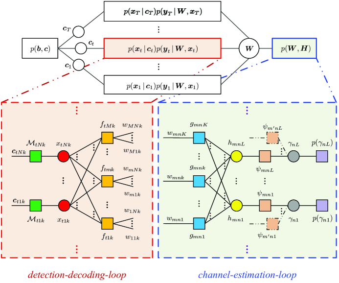
The probabilistic structure defined by the factorizations (13)-(20) can be represented by the factor graph, as depicted in Fig. 1. In this factor graph, mapping constraint δ(φ(𝒄tnk)xtnk)𝛿𝜑subscript𝒄𝑡𝑛𝑘subscript𝑥𝑡𝑛𝑘\delta(\varphi(\boldsymbol{c}_{tnk})-x_{tnk}) appears as a function node tnksubscript𝑡𝑛𝑘\mathcal{M}_{tnk}, the mixing constraint δ(wmnklϕklhmnl)𝛿subscript𝑤𝑚𝑛𝑘subscript𝑙subscriptitalic-ϕ𝑘𝑙subscript𝑚𝑛𝑙\delta(w_{mnk}-\sum_{l}\phi_{kl}h_{mnl}) appears as function node gmnksubscript𝑔𝑚𝑛𝑘g_{mnk}, and the a prior distribution ψ(hmnl,γnl)𝜓subscript𝑚𝑛𝑙subscript𝛾𝑛𝑙\psi(h_{mnl},\gamma_{nl}) appears as function node ψmnlsubscript𝜓𝑚𝑛𝑙\psi_{mnl}.

Refer to caption
Figure 1: Factor graph of the massive MIMO-OFDM system.

There exist two groups of loops, the detection-decoding-loop on the left and the channel-estimation-loop on the right. Unlike a tree-structured factor graph, the existence of loops implies various iterative message passing schedules. In our case, we choose to start passing messages at the channel transition nodes {ftmk}subscript𝑓𝑡𝑚𝑘\{f_{tmk}\}, then pass messages concurrently in both the detection-decoding-loop and the channel-estimation-loop. Each of these full cycles of message passing will be referred to as a “turbo iteration”.

III Expectation Propagation for Joint Channel Estimation And Decoding

The presentation of message passing follows closely with the convention in [13]. Due to high-dimensional integration, directly applying the SPA to the factor graph in Fig. 1 is computationally prohibitive. Hence, we resort to approximate inference to find efficient solutions.

III-A Message Updating in Detection-Decoding-Loop

Note that, to update the outgoing messages from the channel transition node ftmksubscript𝑓𝑡𝑚𝑘f_{tmk}, the received signal shown in (8) can be rewritten as

ytmk=wmnkxtnk+nnwmnkxtnk+ϖtmk,n.subscript𝑦𝑡𝑚𝑘subscript𝑤𝑚𝑛𝑘subscript𝑥𝑡𝑛𝑘subscriptsuperscript𝑛𝑛subscript𝑤𝑚superscript𝑛𝑘subscript𝑥𝑡superscript𝑛𝑘subscriptitalic-ϖ𝑡𝑚𝑘for-all𝑛y_{tmk}=w_{mnk}x_{tnk}+\sum_{n^{\prime}\neq n}w_{mn^{\prime}k}x_{tn^{\prime}k}+\varpi_{tmk},\forall n. (22)

The interference term nnwmnkxtnk+ϖtmksubscriptsuperscript𝑛𝑛subscript𝑤𝑚superscript𝑛𝑘subscript𝑥𝑡superscript𝑛𝑘subscriptitalic-ϖ𝑡𝑚𝑘\sum_{n^{\prime}\neq n}w_{mn^{\prime}k}x_{tn^{\prime}k}+\varpi_{tmk} in (22) is considered as a Gaussian variable [36, 32], and then ytmk(nnwmnkxtnk+ϖtmk)subscript𝑦𝑡𝑚𝑘subscriptsuperscript𝑛𝑛subscript𝑤𝑚superscript𝑛𝑘subscript𝑥𝑡superscript𝑛𝑘subscriptitalic-ϖ𝑡𝑚𝑘y_{tmk}-\bigl{(}\sum_{n^{\prime}\neq n}w_{mn^{\prime}k}x_{tn^{\prime}k}+\varpi_{tmk}\bigr{)} is also a Gaussian variable with the mean zftmkxtnk(i)superscriptsubscript𝑧subscript𝑓𝑡𝑚𝑘subscript𝑥𝑡𝑛𝑘𝑖z_{f_{tmk}\shortrightarrow x_{tnk}}^{(i)} and variance τftmkxtnk(i)superscriptsubscript𝜏subscript𝑓𝑡𝑚𝑘subscript𝑥𝑡𝑛𝑘𝑖\tau_{f_{tmk}\shortrightarrow x_{tnk}}^{(i)} given by

zftmkxtnk(i)superscriptsubscript𝑧subscript𝑓𝑡𝑚𝑘subscript𝑥𝑡𝑛𝑘𝑖\displaystyle z_{f_{tmk}\shortrightarrow x_{tnk}}^{(i)} =ytmknnw^wmnkftmk(i1)x^xtnkftmk(i1),absentsubscript𝑦𝑡𝑚𝑘subscriptsuperscript𝑛𝑛superscriptsubscript^𝑤subscript𝑤𝑚superscript𝑛𝑘subscript𝑓𝑡𝑚𝑘𝑖1superscriptsubscript^𝑥subscript𝑥𝑡superscript𝑛𝑘subscript𝑓𝑡𝑚𝑘𝑖1\displaystyle=y_{tmk}-\sum_{n^{\prime}\neq n}\hat{w}_{w_{mn^{\prime}k}\shortrightarrow f_{tmk}}^{(i-1)}\hat{x}_{x_{tn^{\prime}k}\shortrightarrow f_{tmk}}^{(i-1)}, (23)
τftmkxtnk(i)superscriptsubscript𝜏subscript𝑓𝑡𝑚𝑘subscript𝑥𝑡𝑛𝑘𝑖\displaystyle\tau_{f_{tmk}\shortrightarrow x_{tnk}}^{(i)} =σϖ2+nn(|w^wmnkftmk(i1)|2νxtnkftmk(i1)\displaystyle=\sigma_{\varpi}^{2}+\sum_{n^{\prime}\neq n}\left(\bigl{|}\hat{w}_{w_{mn^{\prime}k}\shortrightarrow f_{tmk}}^{(i-1)}\bigr{|}^{2}\nu_{x_{tn^{\prime}k}\shortrightarrow f_{tmk}}^{(i-1)}\right.
+νwmnkftmk(i1)|x^xtnkftmk(i1)|2+νwmnkftmk(i1)νxtnkftmk(i1)),\displaystyle\left.\hskip 10.00002pt+\nu_{w_{mn^{\prime}k}\shortrightarrow f_{tmk}}^{(i-1)}\bigl{|}\hat{x}_{x_{tn^{\prime}k}\shortrightarrow f_{tmk}}^{(i-1)}\bigr{|}^{2}+\nu_{w_{mn^{\prime}k}\shortrightarrow f_{tmk}}^{(i-1)}\nu_{x_{tn^{\prime}k}\shortrightarrow f_{tmk}}^{(i-1)}\right), (24)

where x^xtnkftmk(i1)superscriptsubscript^𝑥subscript𝑥𝑡𝑛𝑘subscript𝑓𝑡𝑚𝑘𝑖1\hat{x}_{x_{tnk}\shortrightarrow f_{tmk}}^{(i-1)} and νxtnkftmk(i1)superscriptsubscript𝜈subscript𝑥𝑡𝑛𝑘subscript𝑓𝑡𝑚𝑘𝑖1\nu_{x_{tnk}\shortrightarrow f_{tmk}}^{(i-1)} denote the mean and variance of variable xtnksubscript𝑥𝑡𝑛𝑘x_{tnk} with respect to the message μxtnkftmk(i1)(xtnk)superscriptsubscript𝜇subscript𝑥𝑡𝑛𝑘subscript𝑓𝑡𝑚𝑘𝑖1subscript𝑥𝑡𝑛𝑘\mu_{x_{tnk}\shortrightarrow f_{tmk}}^{(i-1)}(x_{tnk}); w^wmnkftmk(i1)superscriptsubscript^𝑤subscript𝑤𝑚𝑛𝑘subscript𝑓𝑡𝑚𝑘𝑖1\hat{w}_{w_{mnk}\shortrightarrow f_{tmk}}^{(i-1)} and νwmnkftmk(i1)superscriptsubscript𝜈subscript𝑤𝑚𝑛𝑘subscript𝑓𝑡𝑚𝑘𝑖1\nu_{w_{mnk}\shortrightarrow f_{tmk}}^{(i-1)} denote the mean and variance of variable wmnksubscript𝑤𝑚𝑛𝑘w_{mnk} with respect to the message μwmnkftmk(i1)(wmnk)superscriptsubscript𝜇subscript𝑤𝑚𝑛𝑘subscript𝑓𝑡𝑚𝑘𝑖1subscript𝑤𝑚𝑛𝑘\mu_{w_{mnk}\shortrightarrow f_{tmk}}^{(i-1)}(w_{mnk}). From the model shown in (22)-(24), the channel transition function ftmksubscript𝑓𝑡𝑚𝑘f_{tmk} at the ith𝑖thi\text{th} turbo iteration can be viewed as

f^tmk(i)(wmnk,xtnk)=𝒩(wmnkxtnk;zftmkxtnk(i),τftmkxtnk(i)),nsuperscriptsubscript^𝑓𝑡𝑚𝑘𝑖subscript𝑤𝑚𝑛𝑘subscript𝑥𝑡𝑛𝑘subscript𝒩subscript𝑤𝑚𝑛𝑘subscript𝑥𝑡𝑛𝑘superscriptsubscript𝑧subscript𝑓𝑡𝑚𝑘subscript𝑥𝑡𝑛𝑘𝑖superscriptsubscript𝜏subscript𝑓𝑡𝑚𝑘subscript𝑥𝑡𝑛𝑘𝑖for-all𝑛\hat{f}_{tmk}^{(i)}(w_{mnk},x_{tnk})=\mathcal{N}_{\mathbb{C}}\left(w_{mnk}x_{tnk};z_{f_{tmk}\shortrightarrow x_{tnk}}^{(i)},\tau_{f_{tmk}\shortrightarrow x_{tnk}}^{(i)}\right),\forall n (25)

Consequently, the message μftmkxtnk(i)(xtnk)superscriptsubscript𝜇subscript𝑓𝑡𝑚𝑘subscript𝑥𝑡𝑛𝑘𝑖subscript𝑥𝑡𝑛𝑘\mu_{f_{tmk}\shortrightarrow x_{tnk}}^{(i)}(x_{tnk}) is calculated by

μftmkxtnk(i)(xtnk)superscriptsubscript𝜇subscript𝑓𝑡𝑚𝑘subscript𝑥𝑡𝑛𝑘𝑖subscript𝑥𝑡𝑛𝑘\displaystyle\mu_{f_{tmk}\shortrightarrow x_{tnk}}^{(i)}(x_{tnk}) =wmnkf^tmk(i)(wmnk,xtnk)μwmnkftmk(i1)(wmnk)absentsubscriptsubscript𝑤𝑚𝑛𝑘superscriptsubscript^𝑓𝑡𝑚𝑘𝑖subscript𝑤𝑚𝑛𝑘subscript𝑥𝑡𝑛𝑘superscriptsubscript𝜇subscript𝑤𝑚𝑛𝑘subscript𝑓𝑡𝑚𝑘𝑖1subscript𝑤𝑚𝑛𝑘\displaystyle=\int_{w_{mnk}}\hat{f}_{tmk}^{(i)}(w_{mnk},x_{tnk})\mu_{w_{mnk}\shortrightarrow f_{tmk}}^{(i-1)}(w_{mnk})
𝒩(xtnk;zftmkxtnk(i)w^wmnkftmk(i1),τftmkxtnk(i)+νwmnkftmk(i1)|xtnk|2|w^wmnkftmk(i1)|2).\displaystyle\propto\mathcal{N}_{\mathbb{C}}\left(x_{tnk};\frac{z_{f_{tmk}\shortrightarrow x_{tnk}}^{\left(i\right)}}{\hat{w}_{w_{mnk}\shortrightarrow f_{tmk}}^{\left(i-1\right)}},\frac{\tau_{f_{tmk}\shortrightarrow x_{tnk}}^{(i)}+\nu_{w_{mnk}\shortrightarrow f_{tmk}}^{\left(i-1\right)}\left|x_{tnk}\right|^{2}}{\bigl{|}\hat{w}_{w_{mnk}\shortrightarrow f_{tmk}}^{\left(i-1\right)}\bigl{|}^{2}}\right). (26)

Using (26), the message from the variable xtnksubscript𝑥𝑡𝑛𝑘x_{tnk} to the channel transition node ftmksubscript𝑓𝑡𝑚𝑘f_{tmk} is updated by

μxtnkftmk(i)(xtnk)=μtnkxtnk(i)(xtnk)𝖾𝗑𝗉(mmΔftmkxtnk(i)(xtnk)),superscriptsubscript𝜇subscript𝑥𝑡𝑛𝑘subscript𝑓𝑡𝑚𝑘𝑖subscript𝑥𝑡𝑛𝑘superscriptsubscript𝜇subscript𝑡𝑛𝑘subscript𝑥𝑡𝑛𝑘𝑖subscript𝑥𝑡𝑛𝑘𝖾𝗑𝗉subscriptsuperscript𝑚𝑚superscriptsubscriptΔsubscript𝑓𝑡superscript𝑚𝑘subscript𝑥𝑡𝑛𝑘𝑖subscript𝑥𝑡𝑛𝑘\mu_{x_{tnk}\shortrightarrow f_{tmk}}^{(i)}\left(x_{tnk}\right)=\mu_{\mathcal{M}_{tnk}\shortrightarrow x_{tnk}}^{(i)}\left(x_{tnk}\right)\mathsf{exp}\left(-\sum_{m^{\prime}\neq m}\Delta_{f_{tm^{\prime}k}\shortrightarrow x_{tnk}}^{(i)}\left(x_{tnk}\right)\right), (27)

where

Δftmkxtnk(i)(xtnk)=|zftmkxtnk(i)w^wmnkftmk(i1)xtnk|2τftmkxtnk(i)+νwmnkftmk(i1)|xtnk|2+𝗅𝗇(τftmkxtnk(i)+νwmnkftmk(i1)|xtnk|2).superscriptsubscriptΔsubscript𝑓𝑡𝑚𝑘subscript𝑥𝑡𝑛𝑘𝑖subscript𝑥𝑡𝑛𝑘superscriptsuperscriptsubscript𝑧subscript𝑓𝑡𝑚𝑘subscript𝑥𝑡𝑛𝑘𝑖superscriptsubscript^𝑤subscript𝑤𝑚𝑛𝑘subscript𝑓𝑡𝑚𝑘𝑖1subscript𝑥𝑡𝑛𝑘2superscriptsubscript𝜏subscript𝑓𝑡𝑚𝑘subscript𝑥𝑡𝑛𝑘𝑖superscriptsubscript𝜈subscript𝑤𝑚𝑛𝑘subscript𝑓𝑡𝑚𝑘𝑖1superscriptsubscript𝑥𝑡𝑛𝑘2𝗅𝗇superscriptsubscript𝜏subscript𝑓𝑡𝑚𝑘subscript𝑥𝑡𝑛𝑘𝑖superscriptsubscript𝜈subscript𝑤𝑚𝑛𝑘subscript𝑓𝑡𝑚𝑘𝑖1superscriptsubscript𝑥𝑡𝑛𝑘2\Delta_{f_{tmk}\shortrightarrow x_{tnk}}^{(i)}\left(x_{tnk}\right)=\frac{\left|z_{f_{tmk}\shortrightarrow x_{tnk}}^{(i)}-\hat{w}_{w_{mnk}\shortrightarrow f_{tmk}}^{\left(i-1\right)}x_{tnk}\right|^{2}}{\tau_{f_{tmk}\shortrightarrow x_{tnk}}^{(i)}+\nu_{w_{mnk}\shortrightarrow f_{tmk}}^{\left(i-1\right)}\left|x_{tnk}\right|^{2}}+\mathsf{ln}\left(\tau_{f_{tmk}\shortrightarrow x_{tnk}}^{(i)}+\nu_{w_{mnk}\shortrightarrow f_{tmk}}^{\left(i-1\right)}\left|x_{tnk}\right|^{2}\right). (28)

To obtain zftmkxtnk(i)superscriptsubscript𝑧subscript𝑓𝑡𝑚𝑘subscript𝑥𝑡𝑛𝑘𝑖z_{f_{tmk}\shortrightarrow x_{tnk}}^{(i)} in (23) and τftmkxtnk(i)superscriptsubscript𝜏subscript𝑓𝑡𝑚𝑘subscript𝑥𝑡𝑛𝑘𝑖\tau_{f_{tmk}\shortrightarrow x_{tnk}}^{(i)} in (24), the mean and variance of variable xtnksubscript𝑥𝑡𝑛𝑘x_{tnk} with respect to the message μxtnkftmk(i1)(xtnk)superscriptsubscript𝜇subscript𝑥𝑡𝑛𝑘subscript𝑓𝑡𝑚𝑘𝑖1subscript𝑥𝑡𝑛𝑘\mu_{x_{tnk}\shortrightarrow f_{tmk}}^{(i-1)}(x_{tnk}) are calculated by

x^xtnkftmk(i1)=αs𝒜αsμxtnkftmk(i1)(xtnk=αs)αs𝒜μxtnkftmk(i1)(xtnk=αs),superscriptsubscript^𝑥subscript𝑥𝑡𝑛𝑘subscript𝑓𝑡𝑚𝑘𝑖1subscriptsubscript𝛼𝑠𝒜subscript𝛼𝑠superscriptsubscript𝜇subscript𝑥𝑡𝑛𝑘subscript𝑓𝑡𝑚𝑘𝑖1subscript𝑥𝑡𝑛𝑘subscript𝛼𝑠subscriptsubscript𝛼𝑠𝒜superscriptsubscript𝜇subscript𝑥𝑡𝑛𝑘subscript𝑓𝑡𝑚𝑘𝑖1subscript𝑥𝑡𝑛𝑘subscript𝛼𝑠\displaystyle\hat{x}_{x_{tnk}\shortrightarrow f_{tmk}}^{\left(i-1\right)}=\frac{\sum_{\alpha_{s}\in\mathcal{A}}\alpha_{s}\mu_{x_{tnk}\shortrightarrow f_{tmk}}^{(i-1)}\left(x_{tnk}=\alpha_{s}\right)}{\sum_{\alpha_{s}\in\mathcal{A}}\mu_{x_{tnk}\shortrightarrow f_{tmk}}^{(i-1)}\left(x_{tnk}=\alpha_{s}\right)}, (29)
νxtnkftmk(i1)=αs𝒜|αs|2μxtnkftmk(i1)(xtnk=αs)αs𝒜μxtnkftmk(i1)(xtnk=αs)|x^xtnkftmk(i1)|2.superscriptsubscript𝜈subscript𝑥𝑡𝑛𝑘subscript𝑓𝑡𝑚𝑘𝑖1subscriptsubscript𝛼𝑠𝒜superscriptsubscript𝛼𝑠2superscriptsubscript𝜇subscript𝑥𝑡𝑛𝑘subscript𝑓𝑡𝑚𝑘𝑖1subscript𝑥𝑡𝑛𝑘subscript𝛼𝑠subscriptsubscript𝛼𝑠𝒜superscriptsubscript𝜇subscript𝑥𝑡𝑛𝑘subscript𝑓𝑡𝑚𝑘𝑖1subscript𝑥𝑡𝑛𝑘subscript𝛼𝑠superscriptsuperscriptsubscript^𝑥subscript𝑥𝑡𝑛𝑘subscript𝑓𝑡𝑚𝑘𝑖12\displaystyle\nu_{x_{tnk}\shortrightarrow f_{tmk}}^{\left(i-1\right)}=\frac{\sum_{\alpha_{s}\in\mathcal{A}}\left|\alpha_{s}\right|^{2}\mu_{x_{tnk}\shortrightarrow f_{tmk}}^{(i-1)}\left(x_{tnk}=\alpha_{s}\right)}{\sum_{\alpha_{s}\in\mathcal{A}}\mu_{x_{tnk}\shortrightarrow f_{tmk}}^{(i-1)}\left(x_{tnk}=\alpha_{s}\right)}-\bigl{|}\hat{x}_{x_{tnk}\shortrightarrow f_{tmk}}^{\left(i-1\right)}\bigr{|}^{2}. (30)

Using the Gaussian approximation shown in (22)-(24) again, the message μftmkwmnk(i)(wmnk)superscriptsubscript𝜇subscript𝑓𝑡𝑚𝑘subscript𝑤𝑚𝑛𝑘𝑖subscript𝑤𝑚𝑛𝑘\mu_{f_{tmk}\shortrightarrow w_{mnk}}^{(i)}\left(w_{mnk}\right) is then updated by

μftmkwmnk(i)(wmnk)xtnk𝒜ϑftmk(i)(xtnk)𝒩(wmnk;zftmkxtnk(i)xtnk,τftmkxtnk(i)|xtnk|2),proportional-tosuperscriptsubscript𝜇subscript𝑓𝑡𝑚𝑘subscript𝑤𝑚𝑛𝑘𝑖subscript𝑤𝑚𝑛𝑘subscriptsubscript𝑥𝑡𝑛𝑘𝒜superscriptsubscriptitalic-ϑsubscript𝑓𝑡𝑚𝑘𝑖subscript𝑥𝑡𝑛𝑘subscript𝒩subscript𝑤𝑚𝑛𝑘superscriptsubscript𝑧subscript𝑓𝑡𝑚𝑘subscript𝑥𝑡𝑛𝑘𝑖subscript𝑥𝑡𝑛𝑘superscriptsubscript𝜏subscript𝑓𝑡𝑚𝑘subscript𝑥𝑡𝑛𝑘𝑖superscriptsubscript𝑥𝑡𝑛𝑘2\mu_{f_{tmk}\shortrightarrow w_{mnk}}^{(i)}\left(w_{mnk}\right)\propto\sum_{x_{tnk}\in\mathcal{A}}\vartheta_{f_{tmk}}^{(i)}\left(x_{tnk}\right)\mathcal{N}_{\mathbb{C}}\left(w_{mnk};\frac{z_{f_{tmk}\shortrightarrow x_{tnk}}^{(i)}}{x_{tnk}},\frac{\tau_{f_{tmk}\shortrightarrow x_{tnk}}^{(i)}}{\left|x_{tnk}\right|^{2}}\right), (31)

where ϑftmk(i)(xtnk)superscriptsubscriptitalic-ϑsubscript𝑓𝑡𝑚𝑘𝑖subscript𝑥𝑡𝑛𝑘\vartheta_{f_{tmk}}^{(i)}\left(x_{tnk}\right) denotes the weight of Gaussian component,

ϑftmk(i)(xtnk)=|xtnk|2μxtnkftmk(i1)(xtnk)xtnk𝒜|xtnk|2μxtnkftmk(i1)(xtnk),xtnk𝒜.formulae-sequencesuperscriptsubscriptitalic-ϑsubscript𝑓𝑡𝑚𝑘𝑖subscript𝑥𝑡𝑛𝑘superscriptsubscript𝑥𝑡𝑛𝑘2superscriptsubscript𝜇subscript𝑥𝑡𝑛𝑘subscript𝑓𝑡𝑚𝑘𝑖1subscript𝑥𝑡𝑛𝑘subscriptsubscript𝑥𝑡𝑛𝑘𝒜superscriptsubscript𝑥𝑡𝑛𝑘2superscriptsubscript𝜇subscript𝑥𝑡𝑛𝑘subscript𝑓𝑡𝑚𝑘𝑖1subscript𝑥𝑡𝑛𝑘subscript𝑥𝑡𝑛𝑘𝒜\vartheta_{f_{tmk}}^{(i)}\left(x_{tnk}\right)=\frac{\left|x_{tnk}\right|^{-2}\mu_{x_{tnk}\shortrightarrow f_{tmk}}^{(i-1)}\left(x_{tnk}\right)}{\sum_{x_{tnk}\in\mathcal{A}}\left|x_{tnk}\right|^{-2}\mu_{x_{tnk}\shortrightarrow f_{tmk}}^{(i-1)}\left(x_{tnk}\right)},x_{tnk}\in\mathcal{A}. (32)

As μftmkwmnk(i)(wmnk)superscriptsubscript𝜇subscript𝑓𝑡𝑚𝑘subscript𝑤𝑚𝑛𝑘𝑖subscript𝑤𝑚𝑛𝑘\mu_{f_{tmk}\shortrightarrow w_{mnk}}^{(i)}\left(w_{mnk}\right) given by (31) is a Gaussian mixture, the number of its components will increase exponentially in the consequent message updating. To avoid the increase, the message μftmkwmnk(i)(wmnk)superscriptsubscript𝜇subscript𝑓𝑡𝑚𝑘subscript𝑤𝑚𝑛𝑘𝑖subscript𝑤𝑚𝑛𝑘\mu_{f_{tmk}\shortrightarrow w_{mnk}}^{(i)}(w_{mnk}) can be projected onto a Gaussian function by the criterion of minimum KL divergence as in [8] and [16]. The projection reduces to matching the first two order moments of a Gaussian function 𝒩(wmnk;w^ftmkwmnk(i),νftmkwmnk(i))subscript𝒩subscript𝑤𝑚𝑛𝑘superscriptsubscript^𝑤subscript𝑓𝑡𝑚𝑘subscript𝑤𝑚𝑛𝑘𝑖superscriptsubscript𝜈subscript𝑓𝑡𝑚𝑘subscript𝑤𝑚𝑛𝑘𝑖\mathcal{N}_{\mathbb{C}}(w_{mnk};\hat{w}_{f_{tmk}\shortrightarrow w_{mnk}}^{(i)},\nu_{f_{tmk}\shortrightarrow w_{mnk}}^{(i)}) and the message μftmkwmnk(i)(wmnk)superscriptsubscript𝜇subscript𝑓𝑡𝑚𝑘subscript𝑤𝑚𝑛𝑘𝑖subscript𝑤𝑚𝑛𝑘\mu_{f_{tmk}\shortrightarrow w_{mnk}}^{(i)}(w_{mnk}) [37], leading to

w^ftmkwmnk(i)superscriptsubscript^𝑤subscript𝑓𝑡𝑚𝑘subscript𝑤𝑚𝑛𝑘𝑖\displaystyle\hat{w}_{f_{tmk}\shortrightarrow w_{mnk}}^{(i)} =zftmkxtnk(i)xtnk𝒜ϑftmk(i)(xtnk)xtnk,absentsuperscriptsubscript𝑧subscript𝑓𝑡𝑚𝑘subscript𝑥𝑡𝑛𝑘𝑖subscriptsubscript𝑥𝑡𝑛𝑘𝒜superscriptsubscriptitalic-ϑsubscript𝑓𝑡𝑚𝑘𝑖subscript𝑥𝑡𝑛𝑘subscript𝑥𝑡𝑛𝑘\displaystyle=z_{f_{tmk}\shortrightarrow x_{tnk}}^{(i)}\sum_{x_{tnk}\in\mathcal{A}}\frac{\vartheta_{f_{tmk}}^{(i)}\left(x_{tnk}\right)}{x_{tnk}}, (33)
νftmkwmnk(i)superscriptsubscript𝜈subscript𝑓𝑡𝑚𝑘subscript𝑤𝑚𝑛𝑘𝑖\displaystyle\nu_{f_{tmk}\shortrightarrow w_{mnk}}^{(i)} =(τftmkxtnk(i)+|zftmkxtnk(i)|2)xtnk𝒜ϑftmk(i)(xtnk)|xtnk|2|w^ftmkwmnk(i)|2.absentsuperscriptsubscript𝜏subscript𝑓𝑡𝑚𝑘subscript𝑥𝑡𝑛𝑘𝑖superscriptsuperscriptsubscript𝑧subscript𝑓𝑡𝑚𝑘subscript𝑥𝑡𝑛𝑘𝑖2subscriptsubscript𝑥𝑡𝑛𝑘𝒜superscriptsubscriptitalic-ϑsubscript𝑓𝑡𝑚𝑘𝑖subscript𝑥𝑡𝑛𝑘superscriptsubscript𝑥𝑡𝑛𝑘2superscriptsuperscriptsubscript^𝑤subscript𝑓𝑡𝑚𝑘subscript𝑤𝑚𝑛𝑘𝑖2\displaystyle=\left(\tau_{f_{tmk}\shortrightarrow x_{tnk}}^{(i)}+\left|z_{f_{tmk}\shortrightarrow x_{tnk}}^{(i)}\right|^{2}\right)\sum_{x_{tnk}\in\mathcal{A}}\frac{\vartheta_{f_{tmk}}^{(i)}(x_{tnk})}{\left|x_{tnk}\right|^{2}}-\left|\hat{w}_{f_{tmk}\shortrightarrow w_{mnk}}^{(i)}\right|^{2}. (34)

The Gaussian approximations shown in (22)-(34) lead to a desirable closed-form message passing algorithm, which will be referred to as “BP-GA”. However, it bears a heavy computations burden: it needs to calculate each μxtnkftmk(i)(xtnk),xtnk𝒜superscriptsubscript𝜇subscript𝑥𝑡𝑛𝑘subscript𝑓𝑡𝑚𝑘𝑖subscript𝑥𝑡𝑛𝑘for-allsubscript𝑥𝑡𝑛𝑘𝒜\mu_{x_{tnk}\shortrightarrow f_{tmk}}^{(i)}(x_{tnk}),\forall x_{tnk}\in\mathcal{A}, but the term mmΔftmkxtnk(i)(xtnk)subscriptsuperscript𝑚𝑚superscriptsubscriptΔsubscript𝑓𝑡superscript𝑚𝑘subscript𝑥𝑡𝑛𝑘𝑖subscript𝑥𝑡𝑛𝑘-\sum_{m^{\prime}\neq m}\Delta_{f_{tm^{\prime}k}\shortrightarrow x_{tnk}}^{(i)}(x_{tnk}) in (27) is complex as M𝑀M is large in the massive MIMO systems. Besides, it needs to calculate each x^xtnkftmk(i1)superscriptsubscript^𝑥subscript𝑥𝑡𝑛𝑘subscript𝑓𝑡𝑚𝑘𝑖1\hat{x}_{x_{tnk}\shortrightarrow f_{tmk}}^{(i-1)} and νxtnkftmk(i1)superscriptsubscript𝜈subscript𝑥𝑡𝑛𝑘subscript𝑓𝑡𝑚𝑘𝑖1\nu_{x_{tnk}\shortrightarrow f_{tmk}}^{(i-1)} using (29) and (30), which amounts to TMNK𝑇𝑀𝑁𝐾TMNK.

Next, we will derive an efficient message-passing algorithm by the framework of expectation propagation. Recalling (22)-(24), a local belief of wmnksubscript𝑤𝑚𝑛𝑘w_{mnk} at the channel-transition function ftmksubscript𝑓𝑡𝑚𝑘f_{tmk} can be defined by

βftmk(i)(wmnk)superscriptsubscript𝛽subscript𝑓𝑡𝑚𝑘𝑖subscript𝑤𝑚𝑛𝑘\displaystyle\beta_{f_{tmk}}^{(i)}\left(w_{mnk}\right) =μwmnkftmk(i1)(wmnk)xtnkf^tmk(i)(wmnk,xtnk)μxtnkftmk(i1)(xtnk)absentsuperscriptsubscript𝜇subscript𝑤𝑚𝑛𝑘subscript𝑓𝑡𝑚𝑘𝑖1subscript𝑤𝑚𝑛𝑘subscriptsubscript𝑥𝑡𝑛𝑘superscriptsubscript^𝑓𝑡𝑚𝑘𝑖subscript𝑤𝑚𝑛𝑘subscript𝑥𝑡𝑛𝑘superscriptsubscript𝜇subscript𝑥𝑡𝑛𝑘subscript𝑓𝑡𝑚𝑘𝑖1subscript𝑥𝑡𝑛𝑘\displaystyle=\mu_{w_{mnk}\shortrightarrow f_{tmk}}^{(i-1)}\left(w_{mnk}\right)\int_{x_{tnk}}\hat{f}_{tmk}^{(i)}(w_{mnk},x_{tnk})\mu_{x_{tnk}\shortrightarrow f_{tmk}}^{(i-1)}\left(x_{tnk}\right)
𝖾𝗑𝗉(Δftmk(i)(wmnk)),n,proportional-toabsent𝖾𝗑𝗉superscriptsubscriptΔsubscript𝑓𝑡𝑚𝑘𝑖subscript𝑤𝑚𝑛𝑘for-all𝑛\displaystyle\propto\mathsf{exp}\left(-\Delta_{f_{tmk}}^{(i)}\left(w_{mnk}\right)\right),\forall n, (35)

where

Δfmnk(i)(wmnk)superscriptsubscriptΔsubscript𝑓𝑚𝑛𝑘𝑖subscript𝑤𝑚𝑛𝑘\displaystyle\Delta_{f_{mnk}}^{(i)}(w_{mnk}) =|zftmkxtnk(i)x^xtnkftmk(i1)wmnk|2τftmkxtnk(i)+νxtnkftmk(i1)|wmnk|2+|wmnkwwmnkftmk(i1)|2νwmnkftmk(i1)absentsuperscriptsuperscriptsubscript𝑧subscript𝑓𝑡𝑚𝑘subscript𝑥𝑡𝑛𝑘𝑖superscriptsubscript^𝑥subscript𝑥𝑡𝑛𝑘subscript𝑓𝑡𝑚𝑘𝑖1subscript𝑤𝑚𝑛𝑘2superscriptsubscript𝜏subscript𝑓𝑡𝑚𝑘subscript𝑥𝑡𝑛𝑘𝑖superscriptsubscript𝜈subscript𝑥𝑡𝑛𝑘subscript𝑓𝑡𝑚𝑘𝑖1superscriptsubscript𝑤𝑚𝑛𝑘2superscriptsubscript𝑤𝑚𝑛𝑘superscriptsubscript𝑤subscript𝑤𝑚𝑛𝑘subscript𝑓𝑡𝑚𝑘𝑖12superscriptsubscript𝜈subscript𝑤𝑚𝑛𝑘subscript𝑓𝑡𝑚𝑘𝑖1\displaystyle=\frac{\left|z_{f_{tmk}\shortrightarrow x_{tnk}}^{(i)}-\hat{x}_{x_{tnk}\shortrightarrow f_{tmk}}^{(i-1)}w_{mnk}\right|^{2}}{\tau_{f_{tmk}\shortrightarrow x_{tnk}}^{(i)}+\nu_{x_{tnk}\shortrightarrow f_{tmk}}^{(i-1)}\left|w_{mnk}\right|^{2}}+\frac{\left|w_{mnk}-w_{w_{mnk}\shortrightarrow f_{tmk}}^{(i-1)}\right|^{2}}{\nu_{w_{mnk}\shortrightarrow f_{tmk}}^{(i-1)}}
+𝗅𝗇(τftmkxtnk(i)+νxtnkftmk(i1)|wmnk|2).𝗅𝗇superscriptsubscript𝜏subscript𝑓𝑡𝑚𝑘subscript𝑥𝑡𝑛𝑘𝑖superscriptsubscript𝜈subscript𝑥𝑡𝑛𝑘subscript𝑓𝑡𝑚𝑘𝑖1superscriptsubscript𝑤𝑚𝑛𝑘2\displaystyle\hskip 10.00002pt+\mathsf{ln}\left(\tau_{f_{tmk}\shortrightarrow x_{tnk}}^{(i)}+\nu_{x_{tnk}\shortrightarrow f_{tmk}}^{(i-1)}\left|w_{mnk}\right|^{2}\right). (36)

We impose a continuous complex Gaussian distribution constraint on the belief of wmnksubscript𝑤𝑚𝑛𝑘w_{mnk}, i.e., we project βftmk(i)(wmnk)superscriptsubscript𝛽subscript𝑓𝑡𝑚𝑘𝑖subscript𝑤𝑚𝑛𝑘\beta_{f_{tmk}}^{(i)}(w_{mnk}) to a Gaussian distribution. The projection reduces to a moment matching; however, the mean and variance of βftmk(i)(wmnk)superscriptsubscript𝛽subscript𝑓𝑡𝑚𝑘𝑖subscript𝑤𝑚𝑛𝑘\beta_{f_{tmk}}^{(i)}(w_{mnk}) involve complex integrals and there are no analytical solutions. So we resort to quadratic approximation for calculating the first two moments of βftmk(i)(wmnk)superscriptsubscript𝛽subscript𝑓𝑡𝑚𝑘𝑖subscript𝑤𝑚𝑛𝑘\beta_{f_{tmk}}^{(i)}(w_{mnk}).

The term zftmkxtnk(i)x^xtnkftmk(i1)wmnksuperscriptsubscript𝑧subscript𝑓𝑡𝑚𝑘subscript𝑥𝑡𝑛𝑘𝑖superscriptsubscript^𝑥subscript𝑥𝑡𝑛𝑘subscript𝑓𝑡𝑚𝑘𝑖1subscript𝑤𝑚𝑛𝑘z_{f_{tmk}\shortrightarrow x_{tnk}}^{(i)}-\hat{x}_{x_{tnk}\shortrightarrow f_{tmk}}^{(i-1)}w_{mnk}, τftmkxtnk(i)+νxtnkftmk(i1)|wmnk|2superscriptsubscript𝜏subscript𝑓𝑡𝑚𝑘subscript𝑥𝑡𝑛𝑘𝑖superscriptsubscript𝜈subscript𝑥𝑡𝑛𝑘subscript𝑓𝑡𝑚𝑘𝑖1superscriptsubscript𝑤𝑚𝑛𝑘2\tau_{f_{tmk}\shortrightarrow x_{tnk}}^{(i)}+\nu_{x_{tnk}\shortrightarrow f_{tmk}}^{(i-1)}\left|w_{mnk}\right|^{2}, and wmnkwwmnkftmk(i1)subscript𝑤𝑚𝑛𝑘superscriptsubscript𝑤subscript𝑤𝑚𝑛𝑘subscript𝑓𝑡𝑚𝑘𝑖1w_{mnk}-w_{w_{mnk}\shortrightarrow f_{tmk}}^{(i-1)} in (36) can be rewritten as

zftmkxtnk(i)x^xtnkftmk(i1)wmnksuperscriptsubscript𝑧subscript𝑓𝑡𝑚𝑘subscript𝑥𝑡𝑛𝑘𝑖superscriptsubscript^𝑥subscript𝑥𝑡𝑛𝑘subscript𝑓𝑡𝑚𝑘𝑖1subscript𝑤𝑚𝑛𝑘\displaystyle z_{f_{tmk}\shortrightarrow x_{tnk}}^{(i)}-\hat{x}_{x_{tnk}\shortrightarrow f_{tmk}}^{(i-1)}w_{mnk} =zftmkxtnk(i)x^xtnkftmk(i1)w^wmnk(i1)z^ftmkwmnk(i)absentsuperscriptsubscript^𝑧subscript𝑓𝑡𝑚𝑘subscript𝑤𝑚𝑛𝑘𝑖superscriptsubscript𝑧subscript𝑓𝑡𝑚𝑘subscript𝑥𝑡𝑛𝑘𝑖superscriptsubscript^𝑥subscript𝑥𝑡𝑛𝑘subscript𝑓𝑡𝑚𝑘𝑖1superscriptsubscript^𝑤subscript𝑤𝑚𝑛𝑘𝑖1\displaystyle=\underset{\hat{z}_{f_{tmk}\shortrightarrow w_{mnk}}^{(i)}}{\underbrace{z_{f_{tmk}\shortrightarrow x_{tnk}}^{(i)}-\hat{x}_{x_{tnk}\shortrightarrow f_{tmk}}^{(i-1)}\hat{w}_{w_{mnk}}^{(i-1)}}}
+x^xtnkftmk(i1)(w^wmnk(i1)wmnk),superscriptsubscript^𝑥subscript𝑥𝑡𝑛𝑘subscript𝑓𝑡𝑚𝑘𝑖1superscriptsubscript^𝑤subscript𝑤𝑚𝑛𝑘𝑖1subscript𝑤𝑚𝑛𝑘\displaystyle\hskip 10.00002pt+\hat{x}_{x_{tnk}\shortrightarrow f_{tmk}}^{(i-1)}\bigl{(}\hat{w}_{w_{mnk}}^{(i-1)}-w_{mnk}\bigr{)}, (37)
τftmkxtnk(i)+νxtnkftmk(i1)|wmnk|2superscriptsubscript𝜏subscript𝑓𝑡𝑚𝑘subscript𝑥𝑡𝑛𝑘𝑖superscriptsubscript𝜈subscript𝑥𝑡𝑛𝑘subscript𝑓𝑡𝑚𝑘𝑖1superscriptsubscript𝑤𝑚𝑛𝑘2\displaystyle\tau_{f_{tmk}\shortrightarrow x_{tnk}}^{(i)}+\nu_{x_{tnk}\shortrightarrow f_{tmk}}^{(i-1)}\left|w_{mnk}\right|^{2} =τftmkxtnk(i)+νxtnkftmk(i1)|w^wmnk(i1)|2τ^ftmkwmnk(i)absentsuperscriptsubscript^𝜏subscript𝑓𝑡𝑚𝑘subscript𝑤𝑚𝑛𝑘𝑖superscriptsubscript𝜏subscript𝑓𝑡𝑚𝑘subscript𝑥𝑡𝑛𝑘𝑖superscriptsubscript𝜈subscript𝑥𝑡𝑛𝑘subscript𝑓𝑡𝑚𝑘𝑖1superscriptsuperscriptsubscript^𝑤subscript𝑤𝑚𝑛𝑘𝑖12\displaystyle=\underset{\hat{\tau}_{f_{tmk}\shortrightarrow w_{mnk}}^{(i)}}{\underbrace{\tau_{f_{tmk}\shortrightarrow x_{tnk}}^{(i)}+\nu_{x_{tnk}\shortrightarrow f_{tmk}}^{(i-1)}\left|\hat{w}_{w_{mnk}}^{(i-1)}\right|^{2}}}
+νxtnkftmk(i1)(|wmnk|2|w^wmnk(i1)|2),superscriptsubscript𝜈subscript𝑥𝑡𝑛𝑘subscript𝑓𝑡𝑚𝑘𝑖1superscriptsubscript𝑤𝑚𝑛𝑘2superscriptsuperscriptsubscript^𝑤subscript𝑤𝑚𝑛𝑘𝑖12\displaystyle\hskip 10.00002pt+\nu_{x_{tnk}\shortrightarrow f_{tmk}}^{(i-1)}\left(\left|w_{mnk}\right|^{2}-\left|\hat{w}_{w_{mnk}}^{(i-1)}\right|^{2}\right), (38)
wmnkw^wmnkftmk(i1)subscript𝑤𝑚𝑛𝑘superscriptsubscript^𝑤subscript𝑤𝑚𝑛𝑘subscript𝑓𝑡𝑚𝑘𝑖1\displaystyle w_{mnk}-\hat{w}_{w_{mnk}\shortrightarrow f_{tmk}}^{(i-1)} =w^wmnk(i1)w^wmnkftmk(i1)+(wmnkw^wmnk(i1)).absentsuperscriptsubscript^𝑤subscript𝑤𝑚𝑛𝑘𝑖1superscriptsubscript^𝑤subscript𝑤𝑚𝑛𝑘subscript𝑓𝑡𝑚𝑘𝑖1subscript𝑤𝑚𝑛𝑘superscriptsubscript^𝑤subscript𝑤𝑚𝑛𝑘𝑖1\displaystyle=\hat{w}_{w_{mnk}}^{(i-1)}-\hat{w}_{w_{mnk}\shortrightarrow f_{tmk}}^{(i-1)}+\left(w_{mnk}-\hat{w}_{w_{mnk}}^{(i-1)}\right). (39)

where w^wmnk(i1)superscriptsubscript^𝑤subscript𝑤𝑚𝑛𝑘𝑖1\hat{w}_{w_{mnk}}^{(i-1)} is the a posteriori mean of wmnksubscript𝑤𝑚𝑛𝑘w_{mnk} at previous turbo iteration. By (84) shown in the Appendix, we can expand Δftmk(i)(xtnk)superscriptsubscriptΔsubscript𝑓𝑡𝑚𝑘𝑖subscript𝑥𝑡𝑛𝑘\Delta_{f_{tmk}}^{(i)}(x_{tnk}) at the point 𝒛0=[z^ftmkwmnk(i),(z^ftmkwmnk(i))]subscript𝒛0superscriptsubscript^𝑧subscript𝑓𝑡𝑚𝑘subscript𝑤𝑚𝑛𝑘𝑖superscriptsuperscriptsubscript^𝑧subscript𝑓𝑡𝑚𝑘subscript𝑤𝑚𝑛𝑘𝑖\vec{\boldsymbol{z}}_{0}=[\hat{z}_{f_{tmk}\shortrightarrow w_{mnk}}^{(i)},(\hat{z}_{f_{tmk}\shortrightarrow w_{mnk}}^{(i)})^{*}], τ0=τ^ftmkwmnk(i)subscript𝜏0superscriptsubscript^𝜏subscript𝑓𝑡𝑚𝑘subscript𝑤𝑚𝑛𝑘𝑖\tau_{0}=\hat{\tau}_{f_{tmk}\shortrightarrow w_{mnk}}^{(i)}, and 𝒖0=[w^wmnk(i1)w^wmnkftmk(i1),(w^wmnk(i1)w^wmnkftmk(i1))]subscript𝒖0superscriptsubscript^𝑤subscript𝑤𝑚𝑛𝑘𝑖1superscriptsubscript^𝑤subscript𝑤𝑚𝑛𝑘subscript𝑓𝑡𝑚𝑘𝑖1superscriptsuperscriptsubscript^𝑤subscript𝑤𝑚𝑛𝑘𝑖1superscriptsubscript^𝑤subscript𝑤𝑚𝑛𝑘subscript𝑓𝑡𝑚𝑘𝑖1\vec{\boldsymbol{u}}_{0}=[\hat{w}_{w_{mnk}}^{(i-1)}-\hat{w}_{w_{mnk}\shortrightarrow f_{tmk}}^{(i-1)},(\hat{w}_{w_{mnk}}^{(i-1)}-\hat{w}_{w_{mnk}\shortrightarrow f_{tmk}}^{(i-1)})^{*}], i.e.,

Δfmnk(i)(wmnk)superscriptsubscriptΔsubscript𝑓𝑚𝑛𝑘𝑖subscript𝑤𝑚𝑛𝑘\displaystyle\Delta_{f_{mnk}}^{(i)}(w_{mnk}) =(1νwmnkftmk(i1)+|x^xtnkftmk(i1)|2τ^ftmkwmnk(i)+νxtnkftmk(i1)τ^ftmkwmnk(i)(1z^ftmkwmnk(i)|2τ^ftmkwmnk(i)))|wmnk|2\displaystyle=\Biggl{(}\frac{1}{\nu_{w_{mnk}\shortrightarrow f_{tmk}}^{(i-1)}}+\frac{\bigl{|}\hat{x}_{x_{tnk}\shortrightarrow f_{tmk}}^{(i-1)}\bigr{|}^{2}}{\hat{\tau}_{f_{tmk}\shortrightarrow w_{mnk}}^{(i)}}+\frac{\nu_{x_{tnk}\shortrightarrow f_{tmk}}^{(i-1)}}{\hat{\tau}_{f_{tmk}\shortrightarrow w_{mnk}}^{(i)}}\biggl{(}1-\frac{\hat{z}_{f_{tmk}\shortrightarrow w_{mnk}}^{(i)}\bigr{|}^{2}}{\hat{\tau}_{f_{tmk}\shortrightarrow w_{mnk}}^{(i)}}\biggr{)}\Biggr{)}\left|w_{mnk}\right|^{2}
2{(zftmkxtnk(i))x^xtnkftmk(i1)τ^ftmkwmnk(i)wmnk+(w^wmnkftmk(i1))νwmnkftmk(i1)wmnk}+𝖼𝗈𝗇𝗌𝗍,2superscriptsuperscriptsubscript𝑧subscript𝑓𝑡𝑚𝑘subscript𝑥𝑡𝑛𝑘𝑖superscriptsubscript^𝑥subscript𝑥𝑡𝑛𝑘subscript𝑓𝑡𝑚𝑘𝑖1superscriptsubscript^𝜏subscript𝑓𝑡𝑚𝑘subscript𝑤𝑚𝑛𝑘𝑖subscript𝑤𝑚𝑛𝑘superscriptsuperscriptsubscript^𝑤subscript𝑤𝑚𝑛𝑘subscript𝑓𝑡𝑚𝑘𝑖1superscriptsubscript𝜈subscript𝑤𝑚𝑛𝑘subscript𝑓𝑡𝑚𝑘𝑖1subscript𝑤𝑚𝑛𝑘𝖼𝗈𝗇𝗌𝗍\displaystyle\hskip 10.00002pt-2\Re\left\{\frac{\bigl{(}z_{f_{tmk}\shortrightarrow x_{tnk}}^{(i)}\bigr{)}^{*}\hat{x}_{x_{tnk}\shortrightarrow f_{tmk}}^{(i-1)}}{\hat{\tau}_{f_{tmk}\shortrightarrow w_{mnk}}^{(i)}}w_{mnk}+\frac{\bigl{(}\hat{w}_{w_{mnk}\shortrightarrow f_{tmk}}^{(i-1)}\bigr{)}^{*}}{\nu_{w_{mnk}\shortrightarrow f_{tmk}}^{(i-1)}}w_{mnk}\right\}+\mathsf{const}, (40)

where the invariant terms with respect to wmnksubscript𝑤𝑚𝑛𝑘w_{mnk} are absorbed into the constant term 𝖼𝗈𝗇𝗌𝗍𝖼𝗈𝗇𝗌𝗍\mathsf{const}. Note that using (40) 𝖾𝗑𝗉{Δfmnk(i)(wmnk)}𝖾𝗑𝗉superscriptsubscriptΔsuperscriptsubscript𝑓𝑚𝑛𝑘𝑖subscript𝑤𝑚𝑛𝑘\mathsf{exp}\{-\Delta_{f_{mn}^{k}}^{(i)}(w_{mnk})\} is essentially the Gaussian approximation of βftmk(i)(wmnk)superscriptsubscript𝛽subscript𝑓𝑡𝑚𝑘𝑖subscript𝑤𝑚𝑛𝑘\beta_{f_{tmk}}^{(i)}(w_{mnk}), i.e.,

βftmk(i)(wmnk)𝒩(wmnk;w^ftmk(i),νftmk(i)),superscriptsubscript𝛽subscript𝑓𝑡𝑚𝑘𝑖subscript𝑤𝑚𝑛𝑘subscript𝒩subscript𝑤𝑚𝑛𝑘superscriptsubscript^𝑤subscript𝑓𝑡𝑚𝑘𝑖superscriptsubscript𝜈subscript𝑓𝑡𝑚𝑘𝑖\beta_{f_{tmk}}^{(i)}(w_{mnk})\approx\mathcal{N}_{\mathbb{C}}\left(w_{mnk};\hat{w}_{f_{tmk}}^{(i)},\nu_{f_{tmk}}^{(i)}\right), (41)

where

νftmk(i)=τ^ftmkwmnk(i)τ^ftmkwmnk(i)νwmnkftmk(i1)+|x^xtnkftmk(i1)|2+νxtnkftmk(i1)(1z^ftmkwmnk(i)|2τ^ftmkwmnk(i)),\displaystyle\nu_{f_{tmk}}^{(i)}=\frac{\hat{\tau}_{f_{tmk}\shortrightarrow w_{mnk}}^{(i)}}{\frac{\hat{\tau}_{f_{tmk}\shortrightarrow w_{mnk}}^{(i)}}{\nu_{w_{mnk}\shortrightarrow f_{tmk}}^{(i-1)}}+\bigl{|}\hat{x}_{x_{tnk}\shortrightarrow f_{tmk}}^{(i-1)}\bigr{|}^{2}+\nu_{x_{tnk}\shortrightarrow f_{tmk}}^{(i-1)}\biggl{(}1-\frac{\hat{z}_{f_{tmk}\shortrightarrow w_{mnk}}^{(i)}\bigr{|}^{2}}{\hat{\tau}_{f_{tmk}\shortrightarrow w_{mnk}}^{(i)}}\biggr{)}}, (42)
w^ftmk(i)=νftmk(i)((x^xtnkftmk(i1))zftmkxtnk(i)τ^ftmkwmnk(i)+w^wmnkftmk(i1)νwmnkftmk(i1)).superscriptsubscript^𝑤subscript𝑓𝑡𝑚𝑘𝑖superscriptsubscript𝜈subscript𝑓𝑡𝑚𝑘𝑖superscriptsuperscriptsubscript^𝑥subscript𝑥𝑡𝑛𝑘subscript𝑓𝑡𝑚𝑘𝑖1superscriptsubscript𝑧subscript𝑓𝑡𝑚𝑘subscript𝑥𝑡𝑛𝑘𝑖superscriptsubscript^𝜏subscript𝑓𝑡𝑚𝑘subscript𝑤𝑚𝑛𝑘𝑖superscriptsubscript^𝑤subscript𝑤𝑚𝑛𝑘subscript𝑓𝑡𝑚𝑘𝑖1superscriptsubscript𝜈subscript𝑤𝑚𝑛𝑘subscript𝑓𝑡𝑚𝑘𝑖1\displaystyle\hat{w}_{f_{tmk}}^{(i)}=\nu_{f_{tmk}}^{(i)}\left(\frac{\left(\hat{x}_{x_{tnk}\shortrightarrow f_{tmk}}^{(i-1)}\right)^{*}z_{f_{tmk}\shortrightarrow x_{tnk}}^{(i)}}{\hat{\tau}_{f_{tmk}\shortrightarrow w_{mnk}}^{(i)}}+\frac{\hat{w}_{w_{mnk}\shortrightarrow f_{tmk}}^{(i-1)}}{\nu_{w_{mnk}\shortrightarrow f_{tmk}}^{(i-1)}}\right). (43)

Using the expectation propagation principle and (41), we get

μftmkwmnk(i)=βftmk(i)(wmnk)μwmnkftmk(i1)𝒩(wmnk;w^ftmkwmnk(i),νftmkwmnk(i)),superscriptsubscript𝜇subscript𝑓𝑡𝑚𝑘subscript𝑤𝑚𝑛𝑘𝑖superscriptsubscript𝛽subscript𝑓𝑡𝑚𝑘𝑖subscript𝑤𝑚𝑛𝑘superscriptsubscript𝜇subscript𝑤𝑚𝑛𝑘subscript𝑓𝑡𝑚𝑘𝑖1proportional-tosubscript𝒩subscript𝑤𝑚𝑛𝑘superscriptsubscript^𝑤subscript𝑓𝑡𝑚𝑘subscript𝑤𝑚𝑛𝑘𝑖superscriptsubscript𝜈subscript𝑓𝑡𝑚𝑘subscript𝑤𝑚𝑛𝑘𝑖\mu_{f_{tmk}\shortrightarrow w_{mnk}}^{(i)}=\frac{\beta_{f_{tmk}}^{(i)}\left(w_{mnk}\right)}{\mu_{w_{mnk}\shortrightarrow f_{tmk}}^{(i-1)}}\propto\mathcal{N}_{\mathbb{C}}\left(w_{mnk};\hat{w}_{f_{tmk}\shortrightarrow w_{mnk}}^{(i)},\nu_{f_{tmk}\shortrightarrow w_{mnk}}^{(i)}\right), (44)

where

νftmkwmnk(i)superscriptsubscript𝜈subscript𝑓𝑡𝑚𝑘subscript𝑤𝑚𝑛𝑘𝑖\displaystyle\nu_{f_{tmk}\shortrightarrow w_{mnk}}^{(i)} =τ^ftmkwmnk(i)|x^xtnkftmk(i1)|2+νxtnkftmk(i1)(1z^ftmkwmnk(i)|2τ^ftmkwmnk(i)),\displaystyle=\frac{\hat{\tau}_{f_{tmk}\shortrightarrow w_{mnk}}^{(i)}}{\bigl{|}\hat{x}_{x_{tnk}\shortrightarrow f_{tmk}}^{(i-1)}\bigr{|}^{2}+\nu_{x_{tnk}\shortrightarrow f_{tmk}}^{(i-1)}\biggl{(}1-\frac{\hat{z}_{f_{tmk}\shortrightarrow w_{mnk}}^{(i)}\bigr{|}^{2}}{\hat{\tau}_{f_{tmk}\shortrightarrow w_{mnk}}^{(i)}}\biggr{)}}, (45)
w^ftmkwmnk(i)superscriptsubscript^𝑤subscript𝑓𝑡𝑚𝑘subscript𝑤𝑚𝑛𝑘𝑖\displaystyle\hat{w}_{f_{tmk}\shortrightarrow w_{mnk}}^{(i)} =νftmkwmnk(i)(x^xtnkftmk(i1))zftmkxtnk(i)τ^ftmkwmnk(i).absentsuperscriptsubscript𝜈subscript𝑓𝑡𝑚𝑘subscript𝑤𝑚𝑛𝑘𝑖superscriptsuperscriptsubscript^𝑥subscript𝑥𝑡𝑛𝑘subscript𝑓𝑡𝑚𝑘𝑖1superscriptsubscript𝑧subscript𝑓𝑡𝑚𝑘subscript𝑥𝑡𝑛𝑘𝑖superscriptsubscript^𝜏subscript𝑓𝑡𝑚𝑘subscript𝑤𝑚𝑛𝑘𝑖\displaystyle=\nu_{f_{tmk}\shortrightarrow w_{mnk}}^{(i)}\frac{\left(\hat{x}_{x_{tnk}\shortrightarrow f_{tmk}}^{(i-1)}\right)^{*}z_{f_{tmk}\shortrightarrow x_{tnk}}^{(i)}}{\hat{\tau}_{f_{tmk}\shortrightarrow w_{mnk}}^{(i)}}. (46)

Note that, the messages at the channel transition nodes associated with known pilot symbol boil down to the following simple form

μftmkwmnk(i)(wmnk)𝒩(wmnk;ytmkxtnk,σϖ2|xtnk|2),(t,k)𝒫n,formulae-sequenceproportional-tosuperscriptsubscript𝜇subscript𝑓𝑡𝑚𝑘subscript𝑤𝑚𝑛𝑘𝑖subscript𝑤𝑚𝑛𝑘subscript𝒩subscript𝑤𝑚𝑛𝑘subscript𝑦𝑡𝑚𝑘subscript𝑥𝑡𝑛𝑘superscriptsubscript𝜎italic-ϖ2superscriptsubscript𝑥𝑡𝑛𝑘2for-all𝑡𝑘subscript𝒫𝑛\mu_{f_{tmk}\shortrightarrow w_{mnk}}^{(i)}(w_{mnk})\propto\mathcal{N}_{\mathbb{C}}\left(w_{mnk};\frac{y_{tmk}}{x_{tnk}},\frac{\sigma_{\varpi}^{2}}{\left|x_{tnk}\right|^{2}}\right),\forall(t,k)\in\mathcal{P}_{n}, (47)

where we use the fact that other users transmit zero-symbols on the pilot subcarriers 𝒫nsubscript𝒫𝑛\mathcal{P}_{n}, and pilot symbol xtnksubscript𝑥𝑡𝑛𝑘x_{tnk} takes a known value.

Similarly, at the channel-transition function ftmksubscript𝑓𝑡𝑚𝑘f_{tmk}, a local belief of xtnksubscript𝑥𝑡𝑛𝑘x_{tnk} can be defined by

βfmnk(i)(xtnk)𝖾𝗑𝗉(Δftmk(i)(xtnk)),proportional-tosuperscriptsubscript𝛽subscript𝑓𝑚𝑛𝑘𝑖subscript𝑥𝑡𝑛𝑘𝖾𝗑𝗉superscriptsubscriptΔsubscript𝑓𝑡𝑚𝑘𝑖subscript𝑥𝑡𝑛𝑘\beta_{f_{mnk}}^{(i)}(x_{tnk})\propto\mathsf{exp}\left(-\Delta_{f_{tmk}}^{(i)}\left(x_{tnk}\right)\right), (48)

where

Δftmk(i)(xtnk)=Δftmkxtnk(i)(xtnk)+|xtnkx^|2xtnkftmk(i1)νxtnkftmk(i1).\Delta_{f_{tmk}}^{(i)}\left(x_{tnk}\right)=\Delta_{f_{tmk}\shortrightarrow x_{tnk}}^{(i)}\left(x_{tnk}\right)+\frac{\left|x_{tnk}-\hat{x}{}_{x_{tnk}\shortrightarrow f_{tmk}}^{(i-1)}\right|^{2}}{\nu_{x_{tnk}\shortrightarrow f_{tmk}}^{(i-1)}}. (49)

The term zftmkxtnk(i)w^wmnkftmk(i1)xtnksuperscriptsubscript𝑧subscript𝑓𝑡𝑚𝑘subscript𝑥𝑡𝑛𝑘𝑖superscriptsubscript^𝑤subscript𝑤𝑚𝑛𝑘subscript𝑓𝑡𝑚𝑘𝑖1subscript𝑥𝑡𝑛𝑘z_{f_{tmk}\shortrightarrow x_{tnk}}^{(i)}-\hat{w}_{w_{mnk}\shortrightarrow f_{tmk}}^{\left(i-1\right)}x_{tnk}, τftmkxtnk(i)+νwmnkftmk(i1)|xtnk|2superscriptsubscript𝜏subscript𝑓𝑡𝑚𝑘subscript𝑥𝑡𝑛𝑘𝑖superscriptsubscript𝜈subscript𝑤𝑚𝑛𝑘subscript𝑓𝑡𝑚𝑘𝑖1superscriptsubscript𝑥𝑡𝑛𝑘2\tau_{f_{tmk}\shortrightarrow x_{tnk}}^{(i)}+\nu_{w_{mnk}\shortrightarrow f_{tmk}}^{\left(i-1\right)}\left|x_{tnk}\right|^{2} and xtnkx^xtnkftmk(i1)x_{tnk}-\hat{x}{}_{x_{tnk}\shortrightarrow f_{tmk}}^{(i-1)} in (49) can also be rewritten as

zftmkxtnk(i)w^wmnkftmk(i1)xtnksuperscriptsubscript𝑧subscript𝑓𝑡𝑚𝑘subscript𝑥𝑡𝑛𝑘𝑖superscriptsubscript^𝑤subscript𝑤𝑚𝑛𝑘subscript𝑓𝑡𝑚𝑘𝑖1subscript𝑥𝑡𝑛𝑘\displaystyle z_{f_{tmk}\shortrightarrow x_{tnk}}^{(i)}-\hat{w}_{w_{mnk}\shortrightarrow f_{tmk}}^{\left(i-1\right)}x_{tnk} =zftmkxtnk(i)w^wmnkftmk(i1)x^xtnk(i1)z^ftmkxtnk(i)absentsuperscriptsubscript^𝑧subscript𝑓𝑡𝑚𝑘subscript𝑥𝑡𝑛𝑘𝑖superscriptsubscript𝑧subscript𝑓𝑡𝑚𝑘subscript𝑥𝑡𝑛𝑘𝑖superscriptsubscript^𝑤subscript𝑤𝑚𝑛𝑘subscript𝑓𝑡𝑚𝑘𝑖1superscriptsubscript^𝑥subscript𝑥𝑡𝑛𝑘𝑖1\displaystyle=\underset{\hat{z}_{f_{tmk}\shortrightarrow x_{tnk}}^{(i)}}{\underbrace{z_{f_{tmk}\shortrightarrow x_{tnk}}^{(i)}-\hat{w}_{w_{mnk}\shortrightarrow f_{tmk}}^{\left(i-1\right)}\hat{x}_{x_{tnk}}^{(i-1)}}}
+w^wmnkftmk(i1)(x^xtnk(i1)xtnk),superscriptsubscript^𝑤subscript𝑤𝑚𝑛𝑘subscript𝑓𝑡𝑚𝑘𝑖1superscriptsubscript^𝑥subscript𝑥𝑡𝑛𝑘𝑖1subscript𝑥𝑡𝑛𝑘\displaystyle\hskip 10.00002pt+\hat{w}_{w_{mnk}\shortrightarrow f_{tmk}}^{\left(i-1\right)}\left(\hat{x}_{x_{tnk}}^{(i-1)}-x_{tnk}\right), (50)
τftmkxtnk(i)+νwmnkftmk(i1)|xtnk|2superscriptsubscript𝜏subscript𝑓𝑡𝑚𝑘subscript𝑥𝑡𝑛𝑘𝑖superscriptsubscript𝜈subscript𝑤𝑚𝑛𝑘subscript𝑓𝑡𝑚𝑘𝑖1superscriptsubscript𝑥𝑡𝑛𝑘2\displaystyle\tau_{f_{tmk}\shortrightarrow x_{tnk}}^{(i)}+\nu_{w_{mnk}\shortrightarrow f_{tmk}}^{\left(i-1\right)}\left|x_{tnk}\right|^{2} =τftmkxtnk(i)+νwmnkftmk(i1)|x^xtnk(i1)|2τ^ftmkxtnk(i)absentsuperscriptsubscript^𝜏subscript𝑓𝑡𝑚𝑘subscript𝑥𝑡𝑛𝑘𝑖superscriptsubscript𝜏subscript𝑓𝑡𝑚𝑘subscript𝑥𝑡𝑛𝑘𝑖superscriptsubscript𝜈subscript𝑤𝑚𝑛𝑘subscript𝑓𝑡𝑚𝑘𝑖1superscriptsuperscriptsubscript^𝑥subscript𝑥𝑡𝑛𝑘𝑖12\displaystyle=\underset{\hat{\tau}_{f_{tmk}\shortrightarrow x_{tnk}}^{(i)}}{\underbrace{\tau_{f_{tmk}\shortrightarrow x_{tnk}}^{(i)}+\nu_{w_{mnk}\shortrightarrow f_{tmk}}^{(i-1)}\left|\hat{x}_{x_{tnk}}^{(i-1)}\right|^{2}}}
+νwmnkftmk(i1)(|xtnk|2|x^xtnk(i1)|2),superscriptsubscript𝜈subscript𝑤𝑚𝑛𝑘subscript𝑓𝑡𝑚𝑘𝑖1superscriptsubscript𝑥𝑡𝑛𝑘2superscriptsuperscriptsubscript^𝑥subscript𝑥𝑡𝑛𝑘𝑖12\displaystyle\hskip 10.00002pt+\nu_{w_{mnk}\shortrightarrow f_{tmk}}^{\left(i-1\right)}\left(\left|x_{tnk}\right|^{2}-\left|\hat{x}_{x_{tnk}}^{(i-1)}\right|^{2}\right), (51)
xtnkx^xtnkftmk(i1)\displaystyle x_{tnk}-\hat{x}{}_{x_{tnk}\shortrightarrow f_{tmk}}^{(i-1)} =x^xtnk(i1)x^+xtnkftmk(i1)(xtnkx^xtnk(i1)),\displaystyle=\hat{x}_{x_{tnk}}^{(i-1)}-\hat{x}{}_{x_{tnk}\shortrightarrow f_{tmk}}^{(i-1)}+\left(x_{tnk}-\hat{x}_{x_{tnk}}^{(i-1)}\right), (52)

where x^xtnk(i1)superscriptsubscript^𝑥subscript𝑥𝑡𝑛𝑘𝑖1\hat{x}_{x_{tnk}}^{(i-1)} is the a posteriori mean of xtnksubscript𝑥𝑡𝑛𝑘x_{tnk} at previous turbo iteration. Then Δftmk(i)(xtnk)superscriptsubscriptΔsubscript𝑓𝑡𝑚𝑘𝑖subscript𝑥𝑡𝑛𝑘\Delta_{f_{tmk}}^{(i)}(x_{tnk}) is expanded at the point at the point 𝒛0=[z^ftmkxtnk(i),(z^ftmkxtnk(i))]subscript𝒛0superscriptsubscript^𝑧subscript𝑓𝑡𝑚𝑘subscript𝑥𝑡𝑛𝑘𝑖superscriptsuperscriptsubscript^𝑧subscript𝑓𝑡𝑚𝑘subscript𝑥𝑡𝑛𝑘𝑖\vec{\boldsymbol{z}}_{0}=[\hat{z}_{f_{tmk}\shortrightarrow x_{tnk}}^{(i)},(\hat{z}_{f_{tmk}\shortrightarrow x_{tnk}}^{(i)})^{*}], τ0=τ^ftmkxtnk(i)subscript𝜏0superscriptsubscript^𝜏subscript𝑓𝑡𝑚𝑘subscript𝑥𝑡𝑛𝑘𝑖\tau_{0}=\hat{\tau}_{f_{tmk}\shortrightarrow x_{tnk}}^{(i)}, and 𝒖0=[x^xtnk(i1)x^,xtnkftmk(i1)(x^xtnk(i1)x^)xtnkftmk(i1)]\vec{\boldsymbol{u}}_{0}=[\hat{x}_{x_{tnk}}^{(i-1)}-\hat{x}{}_{x_{tnk}\shortrightarrow f_{tmk}}^{(i-1)},(\hat{x}_{x_{tnk}}^{(i-1)}-\hat{x}{}_{x_{tnk}\shortrightarrow f_{tmk}}^{(i-1)})^{*}], and we have

μftmkxtnk(i)(xtnk)𝒩(xtnk;x^ftmkxtnk(i),νftmkxtnk(i)),proportional-tosuperscriptsubscript𝜇subscript𝑓𝑡𝑚𝑘subscript𝑥𝑡𝑛𝑘𝑖subscript𝑥𝑡𝑛𝑘subscript𝒩subscript𝑥𝑡𝑛𝑘superscriptsubscript^𝑥subscript𝑓𝑡𝑚𝑘subscript𝑥𝑡𝑛𝑘𝑖superscriptsubscript𝜈subscript𝑓𝑡𝑚𝑘subscript𝑥𝑡𝑛𝑘𝑖\mu_{f_{tmk}\shortrightarrow x_{tnk}}^{(i)}\left(x_{tnk}\right)\propto\mathcal{N}_{\mathbb{C}}\left(x_{tnk};\hat{x}_{f_{tmk}\shortrightarrow x_{tnk}}^{(i)},\nu_{f_{tmk}\shortrightarrow x_{tnk}}^{(i)}\right), (53)

where x^ftmkxtnk(i)superscriptsubscript^𝑥subscript𝑓𝑡𝑚𝑘subscript𝑥𝑡𝑛𝑘𝑖\hat{x}_{f_{tmk}\shortrightarrow x_{tnk}}^{(i)} and νftmkxtnk(i)superscriptsubscript𝜈subscript𝑓𝑡𝑚𝑘subscript𝑥𝑡𝑛𝑘𝑖\nu_{f_{tmk}\shortrightarrow x_{tnk}}^{(i)} are given by

νftmkxtnk(i)superscriptsubscript𝜈subscript𝑓𝑡𝑚𝑘subscript𝑥𝑡𝑛𝑘𝑖\displaystyle\nu_{f_{tmk}\shortrightarrow x_{tnk}}^{(i)} =τ^ftmkxtnk(i)|w^wmnkftmk(i1)|2+νwmnkftmk(i1)(1|z^ftmkxtnk(i)|2τ^ftmkxtnk(i)),absentsuperscriptsubscript^𝜏subscript𝑓𝑡𝑚𝑘subscript𝑥𝑡𝑛𝑘𝑖superscriptsuperscriptsubscript^𝑤subscript𝑤𝑚𝑛𝑘subscript𝑓𝑡𝑚𝑘𝑖12superscriptsubscript𝜈subscript𝑤𝑚𝑛𝑘subscript𝑓𝑡𝑚𝑘𝑖11superscriptsuperscriptsubscript^𝑧subscript𝑓𝑡𝑚𝑘subscript𝑥𝑡𝑛𝑘𝑖2superscriptsubscript^𝜏subscript𝑓𝑡𝑚𝑘subscript𝑥𝑡𝑛𝑘𝑖\displaystyle=\frac{\hat{\tau}_{f_{tmk}\shortrightarrow x_{tnk}}^{(i)}}{\bigl{|}\hat{w}_{w_{mnk}\shortrightarrow f_{tmk}}^{(i-1)}\bigr{|}^{2}+\nu_{w_{mnk}\shortrightarrow f_{tmk}}^{(i-1)}\biggl{(}1-\frac{\left|\hat{z}_{f_{tmk}\shortrightarrow x_{tnk}}^{(i)}\right|^{2}}{\hat{\tau}_{f_{tmk}\shortrightarrow x_{tnk}}^{(i)}}\biggr{)}}, (54)
x^ftmkxtnk(i)superscriptsubscript^𝑥subscript𝑓𝑡𝑚𝑘subscript𝑥𝑡𝑛𝑘𝑖\displaystyle\hat{x}_{f_{tmk}\shortrightarrow x_{tnk}}^{(i)} =νftmkxtnk(i)(w^wmnkftmk(i1))zftmkxtnk(i)τ^ftmkxtnk(i).absentsuperscriptsubscript𝜈subscript𝑓𝑡𝑚𝑘subscript𝑥𝑡𝑛𝑘𝑖superscriptsuperscriptsubscript^𝑤subscript𝑤𝑚𝑛𝑘subscript𝑓𝑡𝑚𝑘𝑖1superscriptsubscript𝑧subscript𝑓𝑡𝑚𝑘subscript𝑥𝑡𝑛𝑘𝑖superscriptsubscript^𝜏subscript𝑓𝑡𝑚𝑘subscript𝑥𝑡𝑛𝑘𝑖\displaystyle=\nu_{f_{tmk}\shortrightarrow x_{tnk}}^{(i)}\frac{\bigl{(}\hat{w}_{w_{mnk}\shortrightarrow f_{tmk}}^{(i-1)}\bigr{)}^{*}z_{f_{tmk}\shortrightarrow x_{tnk}}^{(i)}}{\hat{\tau}_{f_{tmk}\shortrightarrow x_{tnk}}^{(i)}}. (55)

The message μxtnktnk(i)(xtnk)superscriptsubscript𝜇subscript𝑥𝑡𝑛𝑘subscript𝑡𝑛𝑘𝑖subscript𝑥𝑡𝑛𝑘\mu_{x_{tnk}\shortrightarrow\mathcal{M}_{tnk}}^{(i)}(x_{tnk}) from the variable node xtnksubscript𝑥𝑡𝑛𝑘x_{tnk} to the mapper node tnksubscript𝑡𝑛𝑘\mathcal{M}_{tnk} is updated by

μxtnktnk(i)(xtnk)=mμftmkxtnk(i)(xtnk)𝒩(xtnk;ζxtnk(i),γxtnk(i)),superscriptsubscript𝜇subscript𝑥𝑡𝑛𝑘subscript𝑡𝑛𝑘𝑖subscript𝑥𝑡𝑛𝑘subscriptproduct𝑚superscriptsubscript𝜇subscript𝑓𝑡𝑚𝑘subscript𝑥𝑡𝑛𝑘𝑖subscript𝑥𝑡𝑛𝑘proportional-tosubscript𝒩subscript𝑥𝑡𝑛𝑘superscriptsubscript𝜁subscript𝑥𝑡𝑛𝑘𝑖superscriptsubscript𝛾subscript𝑥𝑡𝑛𝑘𝑖\mu_{x_{tnk}\shortrightarrow\mathcal{M}_{tnk}}^{(i)}\left(x_{tnk}\right)=\prod_{m}\mu_{f_{tmk}\shortrightarrow x_{tnk}}^{(i)}\left(x_{tnk}\right)\propto\mathcal{N}_{\mathbb{C}}\left(x_{tnk};\zeta_{x_{tnk}}^{(i)},\gamma_{x_{tnk}}^{(i)}\right), (56)

where γxtnk(i)=1/m(1/νftmkxtnk(i))superscriptsubscript𝛾subscript𝑥𝑡𝑛𝑘𝑖1subscript𝑚1superscriptsubscript𝜈subscript𝑓𝑡𝑚𝑘subscript𝑥𝑡𝑛𝑘𝑖\gamma_{x_{tnk}}^{(i)}=1/\sum_{m}\bigl{(}1/\nu_{f_{tmk}\shortrightarrow x_{tnk}}^{(i)}\bigr{)} and ζxtnk(i)=γxtnk(i)m(x^ftmkxtnk(i)/νftmkxtnk(i))superscriptsubscript𝜁subscript𝑥𝑡𝑛𝑘𝑖superscriptsubscript𝛾subscript𝑥𝑡𝑛𝑘𝑖subscript𝑚superscriptsubscript^𝑥subscript𝑓𝑡𝑚𝑘subscript𝑥𝑡𝑛𝑘𝑖superscriptsubscript𝜈subscript𝑓𝑡𝑚𝑘subscript𝑥𝑡𝑛𝑘𝑖\zeta_{x_{tnk}}^{(i)}=\gamma_{x_{tnk}}^{(i)}\sum_{m}\bigl{(}\hat{x}_{f_{tmk}\shortrightarrow x_{tnk}}^{(i)}/\nu_{f_{tmk}\shortrightarrow x_{tnk}}^{(i)}\bigr{)}. With the message μxtnktnk(i)(xtnk)superscriptsubscript𝜇subscript𝑥𝑡𝑛𝑘subscript𝑡𝑛𝑘𝑖superscriptsubscript𝑥𝑡𝑛𝑘\mu_{x_{tnk}\shortrightarrow\mathcal{M}_{tnk}}^{(i)}(x_{tn}^{k}) and the a priori LLRs {λa(i)(ctnkq),q}superscriptsubscript𝜆𝑎𝑖superscriptsubscript𝑐𝑡𝑛𝑘𝑞for-all𝑞\{\lambda_{a}^{(i)}(c_{tnk}^{q}),\forall q\} fed back by the decoder of user n𝑛n at the previous turbo iteration, the extrinsic LLRs {λe(i)(ctnkq),q}superscriptsubscript𝜆𝑒𝑖superscriptsubscript𝑐𝑡𝑛𝑘𝑞for-all𝑞\{\lambda_{e}^{(i)}(c_{tnk}^{q}),\forall q\} corresponding to the symbol xtnksubscript𝑥𝑡𝑛𝑘x_{tnk} are mapped by

λe(i)(ctnkq)superscriptsubscript𝜆𝑒𝑖superscriptsubscript𝑐𝑡𝑛𝑘𝑞\displaystyle\lambda_{e}^{(i)}\left(c_{tnk}^{q}\right) =𝗅𝗇xtnk𝒜q1μxtnktnk(i)(xtnk)μtnkxtnk(i1)(xtnk)xtnk𝒜q0μxtnktnk(i)(xtnk)μtnkxtnk(i1)(xtnk)λa(i1)(ctnkq),absent𝗅𝗇subscriptsubscript𝑥𝑡𝑛𝑘superscriptsubscript𝒜𝑞1superscriptsubscript𝜇subscript𝑥𝑡𝑛𝑘subscript𝑡𝑛𝑘𝑖subscript𝑥𝑡𝑛𝑘superscriptsubscript𝜇subscript𝑡𝑛𝑘subscript𝑥𝑡𝑛𝑘𝑖1subscript𝑥𝑡𝑛𝑘subscriptsubscript𝑥𝑡𝑛𝑘superscriptsubscript𝒜𝑞0superscriptsubscript𝜇subscript𝑥𝑡𝑛𝑘subscript𝑡𝑛𝑘𝑖subscript𝑥𝑡𝑛𝑘superscriptsubscript𝜇subscript𝑡𝑛𝑘subscript𝑥𝑡𝑛𝑘𝑖1subscript𝑥𝑡𝑛𝑘superscriptsubscript𝜆𝑎𝑖1superscriptsubscript𝑐𝑡𝑛𝑘𝑞\displaystyle=\mathsf{ln}\frac{\sum_{x_{tnk}\in\mathcal{A}_{q}^{1}}\mu_{x_{tnk}\shortrightarrow\mathcal{M}_{tnk}}^{(i)}(x_{tnk})\mu_{\mathcal{M}_{tnk}\shortrightarrow x_{tnk}}^{(i-1)}(x_{tnk})}{\sum_{x_{tnk}\in\mathcal{A}_{q}^{0}}\mu_{x_{tnk}\shortrightarrow\mathcal{M}_{tnk}}^{(i)}(x_{tnk})\mu_{\mathcal{M}_{tnk}\shortrightarrow x_{tnk}}^{(i-1)}(x_{tnk})}-\lambda_{a}^{(i-1)}(c_{tnk}^{q}), (57)

where the (i1)th𝑖1th(i-1)\text{th} message μtnkxtnk(i1)(xtnk)superscriptsubscript𝜇subscript𝑡𝑛𝑘subscript𝑥𝑡𝑛𝑘𝑖1subscript𝑥𝑡𝑛𝑘\mu_{\mathcal{M}_{tnk}\shortrightarrow x_{tnk}}^{(i-1)}(x_{tnk}) is given in the following by (58). Once the extrinsic LLRs {λe(i)(ctnkq)}superscriptsubscript𝜆𝑒𝑖superscriptsubscript𝑐𝑡𝑛𝑘𝑞\{\lambda_{e}^{(i)}(c_{tnk}^{q})\} are available, each channel decoder performs decoding and feeds back the a priori LLRs of coded bits {λa(i)(ctnkq)}superscriptsubscript𝜆𝑎𝑖superscriptsubscript𝑐𝑡𝑛𝑘𝑞\{\lambda_{a}^{(i)}(c_{tnk}^{q})\}, which then are interleaved and converted to the following message

μtnkxtnk(i)(xtnk)=q𝖾𝗑𝗉(ctnkqλa(i)(ctnkq))1+𝖾𝗑𝗉(λa(i)(ctnkq)).superscriptsubscript𝜇subscript𝑡𝑛𝑘subscript𝑥𝑡𝑛𝑘𝑖subscript𝑥𝑡𝑛𝑘subscriptproduct𝑞𝖾𝗑𝗉superscriptsubscript𝑐𝑡𝑛𝑘𝑞superscriptsubscript𝜆𝑎𝑖superscriptsubscript𝑐𝑡𝑛𝑘𝑞1𝖾𝗑𝗉superscriptsubscript𝜆𝑎𝑖superscriptsubscript𝑐𝑡𝑛𝑘𝑞\mu_{\mathcal{M}_{tnk}\shortrightarrow x_{tnk}}^{(i)}\left(x_{tnk}\right)=\prod_{q}\frac{\mathsf{exp}\left(c_{tnk}^{q}\cdot\lambda_{a}^{(i)}\left(c_{tnk}^{q}\right)\right)}{1+\mathsf{exp}\left(\lambda_{a}^{(i)}\left(c_{tnk}^{q}\right)\right)}. (58)

At the variable nodes {xtnk}subscript𝑥𝑡𝑛𝑘\{x_{tnk}\}, the number of message parameters {x^xtnkftmk(i),νxtnkftmk(i)}superscriptsubscript^𝑥subscript𝑥𝑡𝑛𝑘subscript𝑓𝑡𝑚𝑘𝑖superscriptsubscript𝜈subscript𝑥𝑡𝑛𝑘subscript𝑓𝑡𝑚𝑘𝑖\{\hat{x}_{x_{tnk}\shortrightarrow f_{tmk}}^{\left(i\right)},\nu_{x_{tnk}\shortrightarrow f_{tmk}}^{\left(i\right)}\} reaches up to 2TMNK2𝑇𝑀𝑁𝐾2TMNK, so directly evaluating them is expensive via moment matching like (29) and (30). Following the expectation propagation method, we can reduce the computational complexity of {x^xtnkftmk(i),νxtnkftmk(i)}superscriptsubscript^𝑥subscript𝑥𝑡𝑛𝑘subscript𝑓𝑡𝑚𝑘𝑖superscriptsubscript𝜈subscript𝑥𝑡𝑛𝑘subscript𝑓𝑡𝑚𝑘𝑖\{\hat{x}_{x_{tnk}\shortrightarrow f_{tmk}}^{\left(i\right)},\nu_{x_{tnk}\shortrightarrow f_{tmk}}^{\left(i\right)}\}. First, at the variable node xtnksubscript𝑥𝑡𝑛𝑘x_{tnk}, the local belief of xtnksubscript𝑥𝑡𝑛𝑘x_{tnk} is defined by

βxtnk(i)(xtnk)=μtnkxtnk(i)(xtnk)μxtnktnk(i)(xtnk)xtnk𝒜μtnkxtnk(i)(xtnk)μxtnktnk(i)(xtnk).superscriptsubscript𝛽subscript𝑥𝑡𝑛𝑘𝑖subscript𝑥𝑡𝑛𝑘superscriptsubscript𝜇subscript𝑡𝑛𝑘subscript𝑥𝑡𝑛𝑘𝑖subscript𝑥𝑡𝑛𝑘superscriptsubscript𝜇subscript𝑥𝑡𝑛𝑘subscript𝑡𝑛𝑘𝑖subscript𝑥𝑡𝑛𝑘subscriptsubscript𝑥𝑡𝑛𝑘𝒜superscriptsubscript𝜇subscript𝑡𝑛𝑘subscript𝑥𝑡𝑛𝑘𝑖subscript𝑥𝑡𝑛𝑘superscriptsubscript𝜇subscript𝑥𝑡𝑛𝑘subscript𝑡𝑛𝑘𝑖subscript𝑥𝑡𝑛𝑘\beta_{x_{tnk}}^{\left(i\right)}(x_{tnk})=\frac{\mu_{\mathcal{M}_{tnk}\shortrightarrow x_{tnk}}^{(i)}(x_{tnk})\mu_{x_{tnk}\shortrightarrow\mathcal{M}_{tnk}}^{(i)}(x_{tnk})}{\sum_{x_{tnk}\in\mathcal{A}}\mu_{\mathcal{M}_{tnk}\shortrightarrow x_{tnk}}^{(i)}(x_{tnk})\mu_{x_{tnk}\shortrightarrow\mathcal{M}_{tnk}}^{(i)}(x_{tnk})}. (59)

The local belief βxtnk(i)(xtnk)superscriptsubscript𝛽subscript𝑥𝑡𝑛𝑘𝑖subscript𝑥𝑡𝑛𝑘\beta_{x_{tnk}}^{\left(i\right)}(x_{tnk}) can be projected onto a Gaussian PDF denoted by β^xtnk(i)(xtnk)=𝒩(xtnk;x^xtnk(i),νxtnk(i))superscriptsubscript^𝛽subscript𝑥𝑡𝑛𝑘𝑖subscript𝑥𝑡𝑛𝑘subscript𝒩subscript𝑥𝑡𝑛𝑘superscriptsubscript^𝑥subscript𝑥𝑡𝑛𝑘𝑖superscriptsubscript𝜈subscript𝑥𝑡𝑛𝑘𝑖\hat{\beta}_{x_{tnk}}^{\left(i\right)}(x_{tnk})=\mathcal{N}_{\mathbb{C}}\bigl{(}x_{tnk};\hat{x}_{x_{tnk}}^{\left(i\right)},\nu_{x_{tnk}}^{(i)}\bigr{)}, where

x^xtnk(i)superscriptsubscript^𝑥subscript𝑥𝑡𝑛𝑘𝑖\displaystyle\hat{x}_{x_{tnk}}^{\left(i\right)} =αs𝒜αsβxtnk(i)(xtnk=αs),absentsubscriptsubscript𝛼𝑠𝒜subscript𝛼𝑠superscriptsubscript𝛽subscript𝑥𝑡𝑛𝑘𝑖subscript𝑥𝑡𝑛𝑘subscript𝛼𝑠\displaystyle=\sum_{\alpha_{s}\in\mathcal{A}}\alpha_{s}\beta_{x_{tnk}}^{\left(i\right)}\left(x_{tnk}=\alpha_{s}\right), (60)
νxtnk(i)superscriptsubscript𝜈subscript𝑥𝑡𝑛𝑘𝑖\displaystyle\nu_{x_{tnk}}^{(i)} =αs𝒜|αs|2βxtnk(i)(xtnk=αs)|x^xtnk(i)|2,absentsubscriptsubscript𝛼𝑠𝒜superscriptsubscript𝛼𝑠2superscriptsubscript𝛽subscript𝑥𝑡𝑛𝑘𝑖subscript𝑥𝑡𝑛𝑘subscript𝛼𝑠superscriptsuperscriptsubscript^𝑥subscript𝑥𝑡𝑛𝑘𝑖2\displaystyle=\sum_{\alpha_{s}\in\mathcal{A}}\left|\alpha_{s}\right|^{2}\beta_{x_{tnk}}^{\left(i\right)}\left(x_{tnk}=\alpha_{s}\right)-\left|\hat{x}_{x_{tnk}}^{\left(i\right)}\right|^{2}, (61)

and then the message μxtnkftmk(i)(xtnk)superscriptsubscript𝜇subscript𝑥𝑡𝑛𝑘subscript𝑓𝑡𝑚𝑘𝑖subscript𝑥𝑡𝑛𝑘\mu_{x_{tnk}\shortrightarrow f_{tmk}}^{(i)}(x_{tnk}) is approximated by[38]

μ^xtnkftmk(i)(xtnk)superscriptsubscript^𝜇subscript𝑥𝑡𝑛𝑘subscript𝑓𝑡𝑚𝑘𝑖subscript𝑥𝑡𝑛𝑘\displaystyle\hat{\mu}_{x_{tnk}\shortrightarrow f_{tmk}}^{(i)}\left(x_{tnk}\right) β^xtnk(i)(xtnk)μftmkxtnk(i)(xtnk)𝒩(xtnk;x^xtnkftmk(i),νxtnkftmk(i)),absentsuperscriptsubscript^𝛽subscript𝑥𝑡𝑛𝑘𝑖subscript𝑥𝑡𝑛𝑘superscriptsubscript𝜇subscript𝑓𝑡𝑚𝑘subscript𝑥𝑡𝑛𝑘𝑖subscript𝑥𝑡𝑛𝑘proportional-tosubscript𝒩subscript𝑥𝑡𝑛𝑘superscriptsubscript^𝑥subscript𝑥𝑡𝑛𝑘subscript𝑓𝑡𝑚𝑘𝑖superscriptsubscript𝜈subscript𝑥𝑡𝑛𝑘subscript𝑓𝑡𝑚𝑘𝑖\displaystyle\approx\frac{\hat{\beta}_{x_{tnk}}^{\left(i\right)}\left(x_{tnk}\right)}{\mu_{f_{tmk}\shortrightarrow x_{tnk}}^{(i)}\left(x_{tnk}\right)}\propto\mathcal{N}_{\mathbb{C}}\left(x_{tnk};\hat{x}_{x_{tnk}\shortrightarrow f_{tmk}}^{\left(i\right)},\nu_{x_{tnk}\shortrightarrow f_{tmk}}^{\left(i\right)}\right), (62)

where

νxtnkftmk(i)superscriptsubscript𝜈subscript𝑥𝑡𝑛𝑘subscript𝑓𝑡𝑚𝑘𝑖\displaystyle\nu_{x_{tnk}\shortrightarrow f_{tmk}}^{(i)} =νxtnk(i)νftmkxtnk(i)νftmkxtnk(i)νxtnk(i),absentsuperscriptsubscript𝜈subscript𝑥𝑡𝑛𝑘𝑖superscriptsubscript𝜈subscript𝑓𝑡𝑚𝑘subscript𝑥𝑡𝑛𝑘𝑖superscriptsubscript𝜈subscript𝑓𝑡𝑚𝑘subscript𝑥𝑡𝑛𝑘𝑖superscriptsubscript𝜈subscript𝑥𝑡𝑛𝑘𝑖\displaystyle=\nu_{x_{tnk}}^{(i)}\frac{\nu_{f_{tmk}\shortrightarrow x_{tnk}}^{(i)}}{\nu_{f_{tmk}\shortrightarrow x_{tnk}}^{(i)}-\nu_{x_{tnk}}^{(i)}}, (63)
x^xtnkftmk(i)superscriptsubscript^𝑥subscript𝑥𝑡𝑛𝑘subscript𝑓𝑡𝑚𝑘𝑖\displaystyle\hat{x}_{x_{tnk}\shortrightarrow f_{tmk}}^{(i)} =x^xtnk(i)+νxtnk(i)x^xtnk(i)x^ftmkxtnk(i)νftmkxtnk(i)νxtnk(i).absentsuperscriptsubscript^𝑥subscript𝑥𝑡𝑛𝑘𝑖superscriptsubscript𝜈subscript𝑥𝑡𝑛𝑘𝑖superscriptsubscript^𝑥subscript𝑥𝑡𝑛𝑘𝑖superscriptsubscript^𝑥subscript𝑓𝑡𝑚𝑘subscript𝑥𝑡𝑛𝑘𝑖superscriptsubscript𝜈subscript𝑓𝑡𝑚𝑘subscript𝑥𝑡𝑛𝑘𝑖superscriptsubscript𝜈subscript𝑥𝑡𝑛𝑘𝑖\displaystyle=\hat{x}_{x_{tnk}}^{\left(i\right)}+\nu_{x_{tnk}}^{(i)}\frac{\hat{x}_{x_{tnk}}^{\left(i\right)}-\hat{x}_{f_{tmk}\shortrightarrow x_{tnk}}^{(i)}}{\nu_{f_{tmk}\shortrightarrow x_{tnk}}^{(i)}-\nu_{x_{tnk}}^{(i)}}. (64)


t,m,k,n::for-all𝑡𝑚𝑘𝑛absent\displaystyle{\scriptstyle\forall t,m,k,n:} zftmkxtnk(i)=ytmknnw^wmnkftmk(i1)x^xtnkftmk(i1);superscriptsubscript𝑧subscript𝑓𝑡𝑚𝑘subscript𝑥𝑡𝑛𝑘𝑖subscript𝑦𝑡𝑚𝑘subscriptsuperscript𝑛𝑛superscriptsubscript^𝑤subscript𝑤𝑚superscript𝑛𝑘subscript𝑓𝑡𝑚𝑘𝑖1superscriptsubscript^𝑥subscript𝑥𝑡superscript𝑛𝑘subscript𝑓𝑡𝑚𝑘𝑖1\displaystyle{\scriptstyle z_{f_{tmk}\shortrightarrow x_{tnk}}^{(i)}=y_{tmk}-\sum_{n^{\prime}\neq n}\hat{w}_{w_{mn^{\prime}k}\shortrightarrow f_{tmk}}^{(i-1)}\hat{x}_{x_{tn^{\prime}k}\shortrightarrow f_{tmk}}^{(i-1)};}
t,m,k,n::for-all𝑡𝑚𝑘𝑛absent\displaystyle{\scriptstyle\forall t,m,k,n:} τftmkxtnk(i)=σϖ2+nn(|w^wmnkftmk(i1)|2νxtnkftmk(i1)+νwmnkftmk(i1)|x^xtnkftmk(i1)|2+νwmnkftmk(i1)νxtnkftmk(i1))superscriptsubscript𝜏subscript𝑓𝑡𝑚𝑘subscript𝑥𝑡𝑛𝑘𝑖superscriptsubscript𝜎italic-ϖ2subscriptsuperscript𝑛𝑛superscriptsuperscriptsubscript^𝑤subscript𝑤𝑚superscript𝑛𝑘subscript𝑓𝑡𝑚𝑘𝑖12superscriptsubscript𝜈subscript𝑥𝑡superscript𝑛𝑘subscript𝑓𝑡𝑚𝑘𝑖1superscriptsubscript𝜈subscript𝑤𝑚superscript𝑛𝑘subscript𝑓𝑡𝑚𝑘𝑖1superscriptsuperscriptsubscript^𝑥subscript𝑥𝑡superscript𝑛𝑘subscript𝑓𝑡𝑚𝑘𝑖12superscriptsubscript𝜈subscript𝑤𝑚superscript𝑛𝑘subscript𝑓𝑡𝑚𝑘𝑖1superscriptsubscript𝜈subscript𝑥𝑡superscript𝑛𝑘subscript𝑓𝑡𝑚𝑘𝑖1\displaystyle{\scriptstyle\tau_{f_{tmk}\shortrightarrow x_{tnk}}^{(i)}=\sigma_{\varpi}^{2}+\sum_{n^{\prime}\neq n}\Bigl{(}\bigl{|}\hat{w}_{w_{mn^{\prime}k}\shortrightarrow f_{tmk}}^{(i-1)}\bigr{|}^{2}\nu_{x_{tn^{\prime}k}\shortrightarrow f_{tmk}}^{(i-1)}+\nu_{w_{mn^{\prime}k}\shortrightarrow f_{tmk}}^{(i-1)}\bigl{|}\hat{x}_{x_{tn^{\prime}k}\shortrightarrow f_{tmk}}^{(i-1)}\bigr{|}^{2}+\nu_{w_{mn^{\prime}k}\shortrightarrow f_{tmk}}^{(i-1)}\nu_{x_{tn^{\prime}k}\shortrightarrow f_{tmk}}^{(i-1)}\Bigr{)}}
t,m,k,n::for-all𝑡𝑚𝑘𝑛absent\displaystyle{\scriptstyle\forall t,m,k,n:} z^ftmkwmnk(i)=zftmkxtnk(i)x^xtnkftmk(i1)w^wmnk(i1);z^ftmkxtnk(i)=zftmkxtnk(i)w^wmnkftmk(i1)x^xtnk(i1);formulae-sequencesuperscriptsubscript^𝑧subscript𝑓𝑡𝑚𝑘subscript𝑤𝑚𝑛𝑘𝑖superscriptsubscript𝑧subscript𝑓𝑡𝑚𝑘subscript𝑥𝑡𝑛𝑘𝑖superscriptsubscript^𝑥subscript𝑥𝑡𝑛𝑘subscript𝑓𝑡𝑚𝑘𝑖1superscriptsubscript^𝑤subscript𝑤𝑚𝑛𝑘𝑖1superscriptsubscript^𝑧subscript𝑓𝑡𝑚𝑘subscript𝑥𝑡𝑛𝑘𝑖superscriptsubscript𝑧subscript𝑓𝑡𝑚𝑘subscript𝑥𝑡𝑛𝑘𝑖superscriptsubscript^𝑤subscript𝑤𝑚𝑛𝑘subscript𝑓𝑡𝑚𝑘𝑖1superscriptsubscript^𝑥subscript𝑥𝑡𝑛𝑘𝑖1\displaystyle{\scriptstyle\hat{z}_{f_{tmk}\shortrightarrow w_{mnk}}^{(i)}=z_{f_{tmk}\shortrightarrow x_{tnk}}^{(i)}-\hat{x}_{x_{tnk}\shortrightarrow f_{tmk}}^{(i-1)}\hat{w}_{w_{mnk}}^{(i-1)};{\scriptstyle\hat{z}_{f_{tmk}\shortrightarrow x_{tnk}}^{(i)}=z_{f_{tmk}\shortrightarrow x_{tnk}}^{(i)}-\hat{w}_{w_{mnk}\shortrightarrow f_{tmk}}^{\left(i-1\right)}\hat{x}_{x_{tnk}}^{(i-1)};}}
t,m,k,n::for-all𝑡𝑚𝑘𝑛absent\displaystyle{\scriptstyle\forall t,m,k,n:} τ^ftmkwmnk(i)=τftmkxtnk(i)+νxtnkftmk(i1)|w^wmnk(i1)|2;τ^ftmkxtnk(i)=τftmkxtnk(i)+νwmnkftmk(i1)|x^xtnk(i1)|2;formulae-sequencesuperscriptsubscript^𝜏subscript𝑓𝑡𝑚𝑘subscript𝑤𝑚𝑛𝑘𝑖superscriptsubscript𝜏subscript𝑓𝑡𝑚𝑘subscript𝑥𝑡𝑛𝑘𝑖superscriptsubscript𝜈subscript𝑥𝑡𝑛𝑘subscript𝑓𝑡𝑚𝑘𝑖1superscriptsuperscriptsubscript^𝑤subscript𝑤𝑚𝑛𝑘𝑖12superscriptsubscript^𝜏subscript𝑓𝑡𝑚𝑘subscript𝑥𝑡𝑛𝑘𝑖superscriptsubscript𝜏subscript𝑓𝑡𝑚𝑘subscript𝑥𝑡𝑛𝑘𝑖superscriptsubscript𝜈subscript𝑤𝑚𝑛𝑘subscript𝑓𝑡𝑚𝑘𝑖1superscriptsuperscriptsubscript^𝑥subscript𝑥𝑡𝑛𝑘𝑖12\displaystyle{\scriptstyle\hat{\tau}_{f_{tmk}\shortrightarrow w_{mnk}}^{(i)}=\tau_{f_{tmk}\shortrightarrow x_{tnk}}^{(i)}+\nu_{x_{tnk}\shortrightarrow f_{tmk}}^{(i-1)}\bigl{|}\hat{w}_{w_{mnk}}^{(i-1)}\bigr{|}^{2};}{\scriptstyle\hat{\tau}_{f_{tmk}\shortrightarrow x_{tnk}}^{(i)}=\tau_{f_{tmk}\shortrightarrow x_{tnk}}^{(i)}+\nu_{w_{mnk}\shortrightarrow f_{tmk}}^{(i-1)}\bigl{|}\hat{x}_{x_{tnk}}^{(i-1)}\bigr{|}^{2};}
t,m,k,n::for-all𝑡𝑚𝑘𝑛absent\displaystyle{\scriptstyle\forall t,m,k,n:} νftmkxtnk(i)=τ^ftmkxtnk(i)|w^wmnkftmk(i1)|2+νwmnkftmk(i1)(1|z^ftmkxtnk(i)|2τ^ftmkxtnk(i));x^ftmkxtnk(i)=νftmkxtnk(i)(w^wmnkftmk(i1))zftmkxtnk(i)τ^ftmkxtnk(i);formulae-sequencesuperscriptsubscript𝜈subscript𝑓𝑡𝑚𝑘subscript𝑥𝑡𝑛𝑘𝑖superscriptsubscript^𝜏subscript𝑓𝑡𝑚𝑘subscript𝑥𝑡𝑛𝑘𝑖superscriptsuperscriptsubscript^𝑤subscript𝑤𝑚𝑛𝑘subscript𝑓𝑡𝑚𝑘𝑖12superscriptsubscript𝜈subscript𝑤𝑚𝑛𝑘subscript𝑓𝑡𝑚𝑘𝑖11superscriptsuperscriptsubscript^𝑧subscript𝑓𝑡𝑚𝑘subscript𝑥𝑡𝑛𝑘𝑖2superscriptsubscript^𝜏subscript𝑓𝑡𝑚𝑘subscript𝑥𝑡𝑛𝑘𝑖superscriptsubscript^𝑥subscript𝑓𝑡𝑚𝑘subscript𝑥𝑡𝑛𝑘𝑖superscriptsubscript𝜈subscript𝑓𝑡𝑚𝑘subscript𝑥𝑡𝑛𝑘𝑖superscriptsuperscriptsubscript^𝑤subscript𝑤𝑚𝑛𝑘subscript𝑓𝑡𝑚𝑘𝑖1superscriptsubscript𝑧subscript𝑓𝑡𝑚𝑘subscript𝑥𝑡𝑛𝑘𝑖superscriptsubscript^𝜏subscript𝑓𝑡𝑚𝑘subscript𝑥𝑡𝑛𝑘𝑖\displaystyle{\scriptstyle\nu_{f_{tmk}\shortrightarrow x_{tnk}}^{\left(i\right)}=\frac{\hat{\tau}_{f_{tmk}\shortrightarrow x_{tnk}}^{(i)}}{\bigl{|}\hat{w}_{w_{mnk}\shortrightarrow f_{tmk}}^{(i-1)}\bigr{|}^{2}+\nu_{w_{mnk}\shortrightarrow f_{tmk}}^{(i-1)}\biggl{(}1-\frac{\bigl{|}\hat{z}_{f_{tmk}\shortrightarrow x_{tnk}}^{(i)}\bigr{|}^{2}}{\hat{\tau}_{f_{tmk}\shortrightarrow x_{tnk}}^{(i)}}\biggr{)}};}{\scriptstyle\hat{x}_{f_{tmk}\shortrightarrow x_{tnk}}^{\left(i\right)}=\nu_{f_{tmk}\shortrightarrow x_{tnk}}^{(i)}\frac{\bigl{(}\hat{w}_{w_{mnk}\shortrightarrow f_{tmk}}^{(i-1)}\bigr{)}^{*}z_{f_{tmk}\shortrightarrow x_{tnk}}^{(i)}}{\hat{\tau}_{f_{tmk}\shortrightarrow x_{tnk}}^{(i)}};}
t,m,k,n::for-all𝑡𝑚𝑘𝑛absent\displaystyle{\scriptstyle\forall t,m,k,n:} νftmkwmnk(i)=τ^ftmkwmnk(i)|x^xtnkftmk(i1)|2+νxtnkftmk(i1)(1z^ftmkwmnk(i)|2τ^ftmkwmnk(i));w^ftmkwmnk(i)=νftmkwmnk(i)(x^xtnkftmk(i1))zftmkxtnk(i)τ^ftmkwmnk(i);\displaystyle{\scriptstyle\nu_{f_{tmk}\shortrightarrow w_{mnk}}^{\left(i\right)}=\frac{\hat{\tau}_{f_{tmk}\shortrightarrow w_{mnk}}^{(i)}}{\bigl{|}\hat{x}_{x_{tnk}\shortrightarrow f_{tmk}}^{(i-1)}\bigr{|}^{2}+\nu_{x_{tnk}\shortrightarrow f_{tmk}}^{(i-1)}\biggl{(}1-\frac{\hat{z}_{f_{tmk}\shortrightarrow w_{mnk}}^{(i)}\bigr{|}^{2}}{\hat{\tau}_{f_{tmk}\shortrightarrow w_{mnk}}^{(i)}}\biggr{)}};}{\scriptstyle\hat{w}_{f_{tmk}\shortrightarrow w_{mnk}}^{(i)}=\nu_{f_{tmk}\shortrightarrow w_{mnk}}^{(i)}\frac{\bigl{(}\hat{x}_{x_{tnk}\shortrightarrow f_{tmk}}^{(i-1)}\bigr{)}^{*}z_{f_{tmk}\shortrightarrow x_{tnk}}^{(i)}}{\hat{\tau}_{f_{tmk}\shortrightarrow w_{mnk}}^{(i)}};}
t,n,k::for-all𝑡𝑛𝑘absent\displaystyle{\scriptstyle\forall t,n,k:} γxtnk(i)=1m1νftmkxtnk(i);ζxtnk(i)=γxtnk(i)mx^ftmkxtnk(i)νftmkxtnk(i);μxtnktnk(i)(xtnk)=𝒩(xtnk;ζxtnk(i),γxtnk(i));formulae-sequencesuperscriptsubscript𝛾subscript𝑥𝑡𝑛𝑘𝑖1subscript𝑚1superscriptsubscript𝜈subscript𝑓𝑡𝑚𝑘subscript𝑥𝑡𝑛𝑘𝑖formulae-sequencesuperscriptsubscript𝜁subscript𝑥𝑡𝑛𝑘𝑖superscriptsubscript𝛾subscript𝑥𝑡𝑛𝑘𝑖subscript𝑚superscriptsubscript^𝑥subscript𝑓𝑡𝑚𝑘subscript𝑥𝑡𝑛𝑘𝑖superscriptsubscript𝜈subscript𝑓𝑡𝑚𝑘subscript𝑥𝑡𝑛𝑘𝑖superscriptsubscript𝜇subscript𝑥𝑡𝑛𝑘subscript𝑡𝑛𝑘𝑖subscript𝑥𝑡𝑛𝑘subscript𝒩subscript𝑥𝑡𝑛𝑘superscriptsubscript𝜁subscript𝑥𝑡𝑛𝑘𝑖superscriptsubscript𝛾subscript𝑥𝑡𝑛𝑘𝑖\displaystyle{\scriptstyle{\scriptstyle\gamma_{x_{tnk}}^{(i)}}=\frac{1}{\sum_{m}\frac{1}{\nu_{f_{tmk}\shortrightarrow x_{tnk}}^{(i)}}};{\scriptstyle\zeta_{x_{tnk}}^{(i)}}=\gamma_{x_{tnk}}^{(i)}\sum_{m}\frac{\hat{x}_{f_{tmk}\shortrightarrow x_{tnk}}^{(i)}}{\nu_{f_{tmk}\shortrightarrow x_{tnk}}^{(i)}};\mu_{x_{tnk}\shortrightarrow\mathcal{M}_{tnk}}^{(i)}\left(x_{tnk}\right)=\mathcal{N}_{\mathbb{C}}\left(x_{tnk};\zeta_{x_{tnk}}^{(i)},\gamma_{x_{tnk}}^{(i)}\right);}
t,n,k,q::for-all𝑡𝑛𝑘𝑞absent\displaystyle{\scriptstyle\forall t,n,k,q:} λe(i)(ctnkq)=𝗅𝗇xtnk𝒜q1μxtnktnk(i)(xtnk)μtnkxtnk(i1)(xtnk)xtnk𝒜q0μxtnktnk(i)(xtnk)μtnkxtnk(i1)(xtnk)λa(i1)(ctnkq)superscriptsubscript𝜆𝑒𝑖superscriptsubscript𝑐𝑡𝑛𝑘𝑞𝗅𝗇subscriptsuperscriptsubscript𝑥𝑡𝑛𝑘superscriptsubscript𝒜𝑞1superscriptsubscript𝜇subscript𝑥𝑡𝑛𝑘subscript𝑡𝑛𝑘𝑖subscript𝑥𝑡𝑛𝑘superscriptsubscript𝜇subscript𝑡𝑛𝑘subscript𝑥𝑡𝑛𝑘𝑖1subscript𝑥𝑡𝑛𝑘subscriptsuperscriptsubscript𝑥𝑡𝑛𝑘superscriptsubscript𝒜𝑞0superscriptsubscript𝜇subscript𝑥𝑡𝑛𝑘subscript𝑡𝑛𝑘𝑖subscript𝑥𝑡𝑛𝑘superscriptsubscript𝜇subscript𝑡𝑛𝑘subscript𝑥𝑡𝑛𝑘𝑖1subscript𝑥𝑡𝑛𝑘superscriptsubscript𝜆𝑎𝑖1superscriptsubscript𝑐𝑡𝑛𝑘𝑞\displaystyle{\scriptstyle\lambda_{e}^{(i)}(c_{tnk}^{q})=\mathsf{ln}\frac{\sum_{x_{tn}^{k}\in\mathcal{A}_{q}^{1}}\mu_{x_{tnk}\shortrightarrow\mathcal{M}_{tnk}}^{(i)}(x_{tnk})\mu_{\mathcal{M}_{tnk}\shortrightarrow x_{tnk}}^{(i-1)}(x_{tnk})}{\sum_{x_{tn}^{k}\in\mathcal{A}_{q}^{0}}\mu_{x_{tnk}\shortrightarrow\mathcal{M}_{tnk}}^{(i)}(x_{tnk})\mu_{\mathcal{M}_{tnk}\shortrightarrow x_{tnk}}^{(i-1)}(x_{tnk})}-\lambda_{a}^{(i-1)}(c_{tnk}^{q})}
n::for-all𝑛absent\displaystyle{\scriptstyle\forall n:} 𝖣𝖾𝖼𝗈𝖽𝖾𝖺𝗇𝖽𝗀𝖾𝗇𝖾𝗋𝖺𝗍𝖾𝖫𝖫𝖱𝗌{λa(i)(ctnkq),t,k,q}𝖣𝖾𝖼𝗈𝖽𝖾𝖺𝗇𝖽𝗀𝖾𝗇𝖾𝗋𝖺𝗍𝖾𝖫𝖫𝖱𝗌superscriptsubscript𝜆𝑎𝑖superscriptsubscript𝑐𝑡𝑛𝑘𝑞for-all𝑡for-all𝑘for-all𝑞\displaystyle{\scriptstyle\mathsf{Decode}\thinspace\mathsf{and}\thinspace\mathsf{generate}\thinspace\mathsf{LLRs\thinspace}\left\{\lambda_{a}^{(i)}(c_{tnk}^{q}),\forall t,\forall k,\forall q\right\}}
t,n,k::for-all𝑡𝑛𝑘absent\displaystyle{\scriptstyle\forall t,n,k:} μtnkxtnk(i)(xtnk)=q𝖾𝗑𝗉(ctnkqλa(i)(ctnkq))1+𝖾𝗑𝗉(ctnkqλa(i)(ctnkq));βxtnk(i)(xtnk)=μtnkxtnk(i)(xtnk)μxtnktnk(i)(xtnk)xtnk𝒜μtnkxtnk(i)(xtnk)μxtnktnk(i)(xtnk);formulae-sequencesuperscriptsubscript𝜇subscript𝑡𝑛𝑘subscript𝑥𝑡𝑛𝑘𝑖subscript𝑥𝑡𝑛𝑘subscriptproduct𝑞𝖾𝗑𝗉superscriptsubscript𝑐𝑡𝑛𝑘𝑞superscriptsubscript𝜆𝑎𝑖superscriptsubscript𝑐𝑡𝑛𝑘𝑞1𝖾𝗑𝗉superscriptsubscript𝑐𝑡𝑛𝑘𝑞superscriptsubscript𝜆𝑎𝑖superscriptsubscript𝑐𝑡𝑛𝑘𝑞superscriptsubscript𝛽subscript𝑥𝑡𝑛𝑘𝑖subscript𝑥𝑡𝑛𝑘superscriptsubscript𝜇subscript𝑡𝑛𝑘subscript𝑥𝑡𝑛𝑘𝑖subscript𝑥𝑡𝑛𝑘superscriptsubscript𝜇subscript𝑥𝑡𝑛𝑘subscript𝑡𝑛𝑘𝑖subscript𝑥𝑡𝑛𝑘subscriptsubscript𝑥𝑡𝑛𝑘𝒜superscriptsubscript𝜇subscript𝑡𝑛𝑘subscript𝑥𝑡𝑛𝑘𝑖subscript𝑥𝑡𝑛𝑘superscriptsubscript𝜇subscript𝑥𝑡𝑛𝑘subscript𝑡𝑛𝑘𝑖subscript𝑥𝑡𝑛𝑘\displaystyle{\scriptstyle\mu_{\mathcal{M}_{tnk}\shortrightarrow x_{tnk}}^{(i)}(x_{tnk})=\prod_{q}\frac{\mathsf{exp}\bigl{(}c_{tnk}^{q}\lambda_{a}^{(i)}(c_{tnk}^{q})\bigr{)}}{1+\mathsf{exp}\bigl{(}c_{tnk}^{q}\lambda_{a}^{(i)}(c_{tnk}^{q})\bigr{)}};{\scriptstyle{\scriptstyle\beta_{x_{tnk}}^{(i)}\left(x_{tnk}\right)=\frac{\mu_{\mathcal{M}_{tnk}\shortrightarrow x_{tnk}}^{(i)}\left(x_{tnk}\right)\mu_{x_{tnk}\shortrightarrow\mathcal{M}_{tnk}}^{(i)}\left(x_{tnk}\right)}{\sum_{x_{tnk}\in\mathcal{A}}\mu_{\mathcal{M}_{tnk}\shortrightarrow x_{tnk}}^{(i)}(x_{tnk})\mu_{x_{tnk}\shortrightarrow\mathcal{M}_{tnk}}^{(i)}(x_{tnk})}}};}
t,n,k::for-all𝑡𝑛𝑘absent\displaystyle{\scriptstyle\forall t,n,k:} x^xtnk(i)=αs𝒜αsβxtnk(i)(xtnk=αs);νxtnk(i)=αs𝒜|αs|2βxtnk(i)(xtnk=αs)|x^tnk(i)|2;formulae-sequencesuperscriptsubscript^𝑥subscript𝑥𝑡𝑛𝑘𝑖subscriptsubscript𝛼𝑠𝒜subscript𝛼𝑠superscriptsubscript𝛽subscript𝑥𝑡𝑛𝑘𝑖subscript𝑥𝑡𝑛𝑘subscript𝛼𝑠superscriptsubscript𝜈subscript𝑥𝑡𝑛𝑘𝑖subscriptsubscript𝛼𝑠𝒜superscriptsubscript𝛼𝑠2superscriptsubscript𝛽subscript𝑥𝑡𝑛𝑘𝑖subscript𝑥𝑡𝑛𝑘subscript𝛼𝑠superscriptsuperscriptsubscript^𝑥𝑡𝑛𝑘𝑖2\displaystyle{\scriptstyle{\scriptstyle\hat{x}_{x_{tnk}}^{(i)}}=\sum_{\alpha_{s}\in\mathcal{A}}\alpha_{s}\beta_{x_{tnk}}^{(i)}\left(x_{tnk}=\alpha_{s}\right);}{\scriptstyle\nu_{x_{tnk}}^{(i)}}{\scriptstyle=\sum_{\alpha_{s}\in\mathcal{A}}\left|\alpha_{s}\right|^{2}\beta_{x_{tnk}}^{(i)}\left(x_{tnk}=\alpha_{s}\right)-\bigl{|}\hat{x}_{tnk}^{(i)}\bigr{|}^{2};}
t,n,k,m::for-all𝑡𝑛𝑘𝑚absent\displaystyle{\scriptstyle\forall t,n,k,m:} νxtnkftmk(i)=νxtnk(i)νftmkxtnk(i)νftmkxtnk(i)νxtnk(i),m;x^xtnkftmk(i)=x^xtnk(i)+νxtnk(i)x^xtnk(i)x^ftmkxtnk(i)νftmkxtnk(i)νxtnk(i).formulae-sequencesuperscriptsubscript𝜈subscript𝑥𝑡𝑛𝑘subscript𝑓𝑡𝑚𝑘𝑖superscriptsubscript𝜈subscript𝑥𝑡𝑛𝑘𝑖superscriptsubscript𝜈subscript𝑓𝑡𝑚𝑘subscript𝑥𝑡𝑛𝑘𝑖superscriptsubscript𝜈subscript𝑓𝑡𝑚𝑘subscript𝑥𝑡𝑛𝑘𝑖superscriptsubscript𝜈subscript𝑥𝑡𝑛𝑘𝑖for-all𝑚superscriptsubscript^𝑥subscript𝑥𝑡𝑛𝑘subscript𝑓𝑡𝑚𝑘𝑖superscriptsubscript^𝑥subscript𝑥𝑡𝑛𝑘𝑖superscriptsubscript𝜈subscript𝑥𝑡𝑛𝑘𝑖superscriptsubscript^𝑥subscript𝑥𝑡𝑛𝑘𝑖superscriptsubscript^𝑥subscript𝑓𝑡𝑚𝑘subscript𝑥𝑡𝑛𝑘𝑖superscriptsubscript𝜈subscript𝑓𝑡𝑚𝑘subscript𝑥𝑡𝑛𝑘𝑖superscriptsubscript𝜈subscript𝑥𝑡𝑛𝑘𝑖\displaystyle{\scriptstyle\nu_{x_{tnk}\shortrightarrow f_{tmk}}^{(i)}}{\scriptstyle=\nu_{x_{tnk}}^{(i)}\frac{\nu_{f_{tmk}\shortrightarrow x_{tnk}}^{(i)}}{\nu_{f_{tmk}\shortrightarrow x_{tnk}}^{(i)}-\nu_{x_{tnk}}^{(i)}},\forall m;}{\scriptstyle\hat{x}_{x_{tnk}\shortrightarrow f_{tmk}}^{(i)}=\hat{x}_{x_{tnk}}^{\left(i\right)}+\nu_{x_{tnk}}^{(i)}\frac{\hat{x}_{x_{tnk}}^{\left(i\right)}-\hat{x}_{f_{tmk}\shortrightarrow x_{tnk}}^{(i)}}{\nu_{f_{tmk}\shortrightarrow x_{tnk}}^{(i)}-\nu_{x_{tnk}}^{(i)}}.}


Table I: The EP-QA at the ith𝑖thi\text{th} turbo iteration.

Summing up the above discussions, the EP based message passing for the detection-decoding-loop is formulated in Table I, which will be referred to as “EP-QA”. At the first turbo iteration, we set x^xtnkftmk(0)=0,νxtnkftmk(0)=1,t,n,k,mformulae-sequencesuperscriptsubscript^𝑥subscript𝑥𝑡𝑛𝑘subscript𝑓𝑡𝑚𝑘00superscriptsubscript𝜈subscript𝑥𝑡𝑛𝑘subscript𝑓𝑡𝑚𝑘01for-all𝑡𝑛𝑘𝑚\hat{x}_{x_{tnk}\shortrightarrow f_{tmk}}^{(0)}=0,\nu_{x_{tnk}\shortrightarrow f_{tmk}}^{(0)}=1,\forall t,n,k,m; w^wmnkftmk(0)=0,νwmnkftmk(0)=1,t,m,k,nformulae-sequencesuperscriptsubscript^𝑤subscript𝑤𝑚𝑛𝑘subscript𝑓𝑡𝑚𝑘00superscriptsubscript𝜈subscript𝑤𝑚𝑛𝑘subscript𝑓𝑡𝑚𝑘01for-all𝑡𝑚𝑘𝑛\hat{w}_{w_{mnk}\shortrightarrow f_{tmk}}^{(0)}=0,\nu_{w_{mnk}\shortrightarrow f_{tmk}}^{(0)}=1,\forall t,m,k,n; and λa(0)(ctnkq)=0,t,n,k,qsuperscriptsubscript𝜆𝑎0superscriptsubscript𝑐𝑡𝑛𝑘𝑞0for-all𝑡𝑛𝑘𝑞\lambda_{a}^{(0)}(c_{tnk}^{q})=0,\forall t,n,k,q. When updating messages, it can be observed that the variance parameters νftmkwmnk(i)superscriptsubscript𝜈subscript𝑓𝑡𝑚𝑘subscript𝑤𝑚𝑛𝑘𝑖\nu_{f_{tmk}\shortrightarrow w_{mnk}}^{(i)} in (45) and νxtnkftmk(i)superscriptsubscript𝜈subscript𝑥𝑡𝑛𝑘subscript𝑓𝑡𝑚𝑘𝑖\nu_{x_{tnk}\shortrightarrow f_{tmk}}^{(i)} in (63) take negative values in rare situations, which can lead to erratic behavior and is common in many EP implementations [30]. To circumvent this problem, we change a negative νftmkwmnk(i)superscriptsubscript𝜈subscript𝑓𝑡𝑚𝑘subscript𝑤𝑚𝑛𝑘𝑖\nu_{f_{tmk}\shortrightarrow w_{mnk}}^{(i)} to ++\infty ( a large positive constant is used in practice, e.g., 106superscript10610^{6}, see [39] and [40]) and change a negative νxtnkftmk(i)superscriptsubscript𝜈subscript𝑥𝑡𝑛𝑘subscript𝑓𝑡𝑚𝑘𝑖\nu_{x_{tnk}\shortrightarrow f_{tmk}}^{(i)} to νxtnk(i)superscriptsubscript𝜈subscript𝑥𝑡𝑛𝑘𝑖\nu_{x_{tnk}}^{(i)} shown in (61). Although this is just a heuristic measure, in our simulations it indeed avoids the instability of expectation propagation.

III-B Message Updating in Channel-Estimation-Loop


m,n,k:zgmnk(i)=w^wmnkgmnk(i)lϕklh^hmnl(i1)+ϵmnk(i1);τgmnk(i)=νwmnkgmnk(i)+lνhmnl(i1).mn:τ¯mn(i)=kτgmnk(i)/K.m,n,l:ξmnl(i)=kΦklzgmnk(i)τgmnk(i)+h^hmnl(i1)k1τgmnk(i)νhmnl(i1)τ¯mn(i)ξmnl(i1);νhmnl(i)=1Mm(|h^hmnl(i1)|2+νhmnl(i1))+k1τgmnk(i);h^hmnl(i)=νhmnl(i)ξmnl(i).mn:ν¯mn(i)=lνhmnl(i)/L.m,n,k:ϵmnk(i)=zgmnk(i)lνhmnl(i)+lϕklνhmnl(i)h^hmnl(i1)ν¯mn(i)ϵmnk(i1)τgmnk(i);w^gmnkwmnk(i)=lϕklh^hmnl(i)ϵmnk(i);νgmnkwmnk(i)=lνhmnl(i).m,n,k:νwmnk(i)=11νgmnkwmnk(i)+t1νftmkwmnk(i),w^wmnk(i)=νwmnk(i)(w^gmnkwmnk(i)νgmnkwmnk(i)+tw^ftmkwmnk(i)νftmkwmnk(i)).m,n,k,t:νwmnkftmk(i)=11νwmnk(i)1νftmkwmnk(i),w^wmnkftmk(i)=νwmnkftmk(i)(νwmnk(i)w^wmnk(i)w^ftmkwmnk(i)νftmkwmnk(i)).:for-all𝑚𝑛𝑘absentformulae-sequencesuperscriptsubscript𝑧subscript𝑔𝑚𝑛𝑘𝑖superscriptsubscript^𝑤subscript𝑤𝑚𝑛𝑘subscript𝑔𝑚𝑛𝑘𝑖subscript𝑙subscriptitalic-ϕ𝑘𝑙superscriptsubscript^subscript𝑚𝑛𝑙𝑖1superscriptsubscriptitalic-ϵ𝑚𝑛𝑘𝑖1superscriptsubscript𝜏subscript𝑔𝑚𝑛𝑘𝑖superscriptsubscript𝜈subscript𝑤𝑚𝑛𝑘subscript𝑔𝑚𝑛𝑘𝑖subscript𝑙superscriptsubscript𝜈subscript𝑚𝑛𝑙𝑖1:for-all𝑚𝑛absentsuperscriptsubscript¯𝜏𝑚𝑛𝑖subscript𝑘superscriptsubscript𝜏subscript𝑔𝑚𝑛𝑘𝑖𝐾:for-all𝑚𝑛𝑙absentformulae-sequencesuperscriptsubscript𝜉𝑚𝑛𝑙𝑖subscript𝑘superscriptsubscriptΦ𝑘𝑙superscriptsubscript𝑧subscript𝑔𝑚𝑛𝑘𝑖superscriptsubscript𝜏subscript𝑔𝑚𝑛𝑘𝑖superscriptsubscript^subscript𝑚𝑛𝑙𝑖1subscriptsuperscript𝑘1superscriptsubscript𝜏subscript𝑔𝑚𝑛superscript𝑘𝑖superscriptsubscript𝜈subscript𝑚𝑛𝑙𝑖1superscriptsubscript¯𝜏𝑚𝑛𝑖superscriptsubscript𝜉𝑚𝑛𝑙𝑖1formulae-sequencesuperscriptsubscript𝜈subscript𝑚𝑛𝑙𝑖1𝑀subscriptsuperscript𝑚superscriptsuperscriptsubscript^subscriptsuperscript𝑚𝑛𝑙𝑖12superscriptsubscript𝜈subscriptsuperscript𝑚𝑛𝑙𝑖1subscript𝑘1superscriptsubscript𝜏subscript𝑔𝑚𝑛𝑘𝑖superscriptsubscript^subscript𝑚𝑛𝑙𝑖superscriptsubscript𝜈subscript𝑚𝑛𝑙𝑖superscriptsubscript𝜉𝑚𝑛𝑙𝑖:for-all𝑚𝑛absentsuperscriptsubscript¯𝜈𝑚𝑛𝑖subscript𝑙superscriptsubscript𝜈subscript𝑚𝑛𝑙𝑖𝐿:for-all𝑚𝑛𝑘absentformulae-sequencesuperscriptsubscriptitalic-ϵ𝑚𝑛𝑘𝑖superscriptsubscript𝑧subscript𝑔𝑚𝑛𝑘𝑖subscript𝑙superscriptsubscript𝜈subscript𝑚𝑛𝑙𝑖subscriptsuperscript𝑙subscriptitalic-ϕ𝑘superscript𝑙superscriptsubscript𝜈subscript𝑚𝑛superscript𝑙𝑖superscriptsubscript^subscript𝑚𝑛superscript𝑙𝑖1superscriptsubscript¯𝜈𝑚𝑛𝑖superscriptsubscriptitalic-ϵ𝑚𝑛𝑘𝑖1superscriptsubscript𝜏subscript𝑔𝑚𝑛𝑘𝑖formulae-sequencesuperscriptsubscript^𝑤subscript𝑔𝑚𝑛𝑘subscript𝑤𝑚𝑛𝑘𝑖subscript𝑙subscriptitalic-ϕ𝑘𝑙superscriptsubscript^subscript𝑚𝑛𝑙𝑖superscriptsubscriptitalic-ϵ𝑚𝑛𝑘𝑖superscriptsubscript𝜈subscript𝑔𝑚𝑛𝑘subscript𝑤𝑚𝑛𝑘𝑖subscript𝑙superscriptsubscript𝜈subscript𝑚𝑛𝑙𝑖:for-all𝑚𝑛𝑘absentformulae-sequencesuperscriptsubscript𝜈subscript𝑤𝑚𝑛𝑘𝑖11superscriptsubscript𝜈subscript𝑔𝑚𝑛𝑘subscript𝑤𝑚𝑛𝑘𝑖subscript𝑡1superscriptsubscript𝜈subscript𝑓𝑡𝑚𝑘subscript𝑤𝑚𝑛𝑘𝑖superscriptsubscript^𝑤subscript𝑤𝑚𝑛𝑘𝑖superscriptsubscript𝜈subscript𝑤𝑚𝑛𝑘𝑖superscriptsubscript^𝑤subscript𝑔𝑚𝑛𝑘subscript𝑤𝑚𝑛𝑘𝑖superscriptsubscript𝜈subscript𝑔𝑚𝑛𝑘subscript𝑤𝑚𝑛𝑘𝑖subscript𝑡superscriptsubscript^𝑤subscript𝑓𝑡𝑚𝑘subscript𝑤𝑚𝑛𝑘𝑖superscriptsubscript𝜈subscript𝑓𝑡𝑚𝑘subscript𝑤𝑚𝑛𝑘𝑖:for-all𝑚𝑛𝑘𝑡absentformulae-sequencesuperscriptsubscript𝜈subscript𝑤𝑚𝑛𝑘subscript𝑓𝑡𝑚𝑘𝑖11superscriptsubscript𝜈subscript𝑤𝑚𝑛𝑘𝑖1superscriptsubscript𝜈subscript𝑓𝑡𝑚𝑘subscript𝑤𝑚𝑛𝑘𝑖superscriptsubscript^𝑤subscript𝑤𝑚𝑛𝑘subscript𝑓𝑡𝑚𝑘𝑖superscriptsubscript𝜈subscript𝑤𝑚𝑛𝑘subscript𝑓𝑡𝑚𝑘𝑖superscriptsubscript𝜈subscript𝑤𝑚𝑛𝑘𝑖superscriptsubscript^𝑤subscript𝑤𝑚𝑛𝑘𝑖superscriptsubscript^𝑤subscript𝑓𝑡𝑚𝑘subscript𝑤𝑚𝑛𝑘𝑖superscriptsubscript𝜈subscript𝑓𝑡𝑚𝑘subscript𝑤𝑚𝑛𝑘𝑖\begin{aligned} {\scriptstyle\forall m,n,k:}&{\scriptstyle z_{g_{mnk}}^{(i)}=\hat{w}_{w_{mnk}\shortrightarrow g_{mnk}}^{(i)}-\sum_{l}\phi_{kl}\hat{h}_{h_{mnl}}^{(i-1)}+\epsilon_{mnk}^{(i-1)};\tau_{g_{mnk}}^{(i)}=\nu_{w_{mnk}\shortrightarrow g_{mnk}}^{(i)}+\sum_{l}\nu_{h_{mnl}}^{(i-1)}.}\\ {\scriptstyle\forall mn:}&{\scriptstyle\bar{\tau}_{mn}^{(i)}=\sum_{k}\tau_{g_{mnk}}^{(i)}/K.}\\ {\scriptstyle\forall m,n,l:}&{\scriptstyle\xi_{mnl}^{(i)}=\sum_{k}\frac{\varPhi_{kl}^{*}z_{g_{mnk}}^{(i)}}{\tau_{g_{mnk}}^{(i)}}+\hat{h}_{h_{mnl}}^{(i-1)}\sum_{k^{\prime}}\frac{1}{\tau_{g_{mnk^{\prime}}}^{(i)}}-\frac{\nu_{h_{mnl}}^{(i-1)}}{\bar{\tau}_{mn}^{(i)}}\xi_{mnl}^{(i-1)};\nu_{h_{mnl}}^{(i)}=\frac{1}{\frac{M}{\sum_{m^{\prime}}\biggl{(}\Bigl{|}\hat{h}_{h_{m^{\prime}nl}}^{(i-1)}\Bigr{|}^{2}+\nu_{h_{m^{\prime}nl}}^{(i-1)}\biggr{)}}+\sum_{k}\frac{1}{\tau_{g_{mnk}}^{(i)}}};\hat{h}_{h_{mnl}}^{(i)}=\nu_{h_{mnl}}^{(i)}\xi_{mnl}^{(i)}.}\\ {\scriptstyle\forall mn:}&{\scriptstyle\bar{\nu}_{mn}^{(i)}=\sum_{l}\nu_{h_{mnl}}^{(i)}/L.}\\ {\scriptstyle\forall m,n,k:}&{\scriptstyle\epsilon_{mnk}^{(i)}=\frac{z_{g_{mnk}}^{(i)}\sum_{l}\nu_{h_{mnl}}^{(i)}+\sum_{l^{\prime}}\phi_{kl^{\prime}}\nu_{h_{mnl^{\prime}}}^{(i)}\hat{h}_{h_{mnl^{\prime}}}^{(i-1)}-\bar{\nu}_{mn}^{(i)}\epsilon_{mnk}^{(i-1)}}{\tau_{g_{mnk}}^{(i)}};{\scriptstyle\hat{w}_{g_{mnk}\shortrightarrow w_{mnk}}^{(i)}=\sum_{l}\phi_{kl}\hat{h}_{h_{mnl}}^{(i)}-\epsilon_{mnk}^{(i)};}\nu_{g_{mnk}\shortrightarrow w_{mnk}}^{(i)}=\sum_{l}\nu_{h_{mnl}}^{(i)}.}\\ {\scriptstyle\forall m,n,k:}&{\scriptstyle\nu_{w_{mnk}}^{(i)}=\frac{1}{\frac{1}{\nu_{g_{mnk}\shortrightarrow w_{mnk}}^{(i)}}+\sum_{t}\frac{1}{\nu_{f_{tmk}\shortrightarrow w_{mnk}}^{(i)}}},\hat{w}_{w_{mnk}}^{(i)}=\nu_{w_{mnk}}^{(i)}\Biggl{(}\frac{\hat{w}_{g_{mnk}\shortrightarrow w_{mnk}}^{(i)}}{\nu_{g_{mnk}\shortrightarrow w_{mnk}}^{(i)}}+\sum_{t}\frac{\hat{w}_{f_{tmk}\shortrightarrow w_{mnk}}^{(i)}}{\nu_{f_{tmk}\shortrightarrow w_{mnk}}^{(i)}}\Biggr{)}.}\\ {\scriptstyle\forall m,n,k,t:}&{\scriptstyle\nu_{w_{mnk}\shortrightarrow f_{tmk}}^{(i)}=\frac{1}{\frac{1}{\nu_{w_{mnk}}^{(i)}}-\frac{1}{\nu_{f_{tmk}\shortrightarrow w_{mnk}}^{(i)}}},\hat{w}_{w_{mnk}\shortrightarrow f_{tmk}}^{(i)}=\nu_{w_{mnk}\shortrightarrow f_{tmk}}^{(i)}\Biggl{(}\frac{\nu_{w_{mnk}}^{(i)}}{\hat{w}_{w_{mnk}}^{(i)}}-\frac{\hat{w}_{f_{tmk}\shortrightarrow w_{mnk}}^{(i)}}{\nu_{f_{tmk}\shortrightarrow w_{mnk}}^{(i)}}\Biggr{)}.}\end{aligned}


Table II: The GMP at the ith𝑖thi\text{th} turbo iteration.

Now we focus on Bayesian learning of the hyper-parameters {γnl}subscript𝛾𝑛𝑙\{\gamma_{nl}\}, as it is unknown to the receiver. Using the variational message-passing rule [41], we obtain the message from the function node ψmnlsubscript𝜓𝑚𝑛𝑙\psi_{mnl} to the precision variable γnlsubscript𝛾𝑛𝑙\gamma_{nl},

μψmnlγnl(i)(γnl)=𝖾𝗑𝗉(𝖤βhmnl(i1)(hmnl)𝗅𝗇ψmnl(hmnl,γnl))𝖦𝖺𝗆(γnl;0,|h^hmnl(i1)|2+νhmnl(i1)),superscriptsubscript𝜇subscript𝜓𝑚𝑛𝑙subscript𝛾𝑛𝑙𝑖subscript𝛾𝑛𝑙𝖾𝗑𝗉subscript𝖤superscriptsubscript𝛽subscript𝑚𝑛𝑙𝑖1subscript𝑚𝑛𝑙𝗅𝗇subscript𝜓𝑚𝑛𝑙subscript𝑚𝑛𝑙subscript𝛾𝑛𝑙proportional-to𝖦𝖺𝗆subscript𝛾𝑛𝑙0superscriptsuperscriptsubscript^subscript𝑚𝑛𝑙𝑖12superscriptsubscript𝜈subscript𝑚𝑛𝑙𝑖1\mu_{\psi_{mnl}\shortrightarrow\gamma_{nl}}^{(i)}(\gamma_{nl})=\mathsf{exp}\biggl{(}\mathsf{E}_{\beta_{h_{mnl}}^{(i-1)}\left(h_{mnl}\right)}\mathsf{ln}\psi_{mnl}\left(h_{mnl},\gamma_{nl}\right)\biggr{)}\propto\mathsf{Gam}\Bigl{(}\gamma_{nl};0,\bigl{|}\hat{h}_{h_{mnl}}^{(i-1)}\bigr{|}^{2}+\nu_{h_{mnl}}^{(i-1)}\Bigr{)}, (65)

where βhmnl(i1)(hmnl)=𝒩(hmnl;h^hmnl(i1),νhmnl(i1))superscriptsubscript𝛽subscript𝑚𝑛𝑙𝑖1subscript𝑚𝑛𝑙subscript𝒩subscript𝑚𝑛𝑙superscriptsubscript^subscript𝑚𝑛𝑙𝑖1superscriptsubscript𝜈subscript𝑚𝑛𝑙𝑖1\beta_{h_{mnl}}^{(i-1)}(h_{mnl})=\mathcal{N}_{\mathbb{C}}\Bigl{(}h_{mnl};\hat{h}_{h_{mnl}}^{(i-1)},\nu_{h_{mnl}}^{(i-1)}\Bigr{)} is the belief of hmnlsubscript𝑚𝑛𝑙h_{mnl} at the (i1)th𝑖1th\left(i-1\right)\text{th} turbo iteration. Then the belief of precision variable γnlsubscript𝛾𝑛𝑙\gamma_{nl} is updated by

βγnl(i)(γnl)=p(γnl)mμψmnlγnl(i)(γnl)𝖦𝖺𝗆(γnl;M,m(|h^hmnl(i1)|2+νhmnl(i1))),superscriptsubscript𝛽subscript𝛾𝑛𝑙𝑖subscript𝛾𝑛𝑙𝑝subscript𝛾𝑛𝑙subscriptproduct𝑚superscriptsubscript𝜇subscript𝜓𝑚𝑛𝑙subscript𝛾𝑛𝑙𝑖subscript𝛾𝑛𝑙proportional-to𝖦𝖺𝗆subscript𝛾𝑛𝑙𝑀subscript𝑚superscriptsuperscriptsubscript^subscript𝑚𝑛𝑙𝑖12superscriptsubscript𝜈subscript𝑚𝑛𝑙𝑖1\beta_{\gamma_{nl}}^{(i)}(\gamma_{nl})=p(\gamma_{nl})\prod_{m}\mu_{\psi_{mnl}\shortrightarrow\gamma_{nl}}^{(i)}(\gamma_{nl})\propto\mathsf{Gam}\biggl{(}\gamma_{nl};M,\sum_{m}\Bigl{(}\bigl{|}\hat{h}_{h_{mnl}}^{(i-1)}\bigr{|}^{2}+\nu_{h_{mnl}}^{(i-1)}\Bigr{)}\biggr{)}, (66)

Using the variational message-passing rule again, the message from the function node ψmnl(hmnl,γnl)subscript𝜓𝑚𝑛𝑙subscript𝑚𝑛𝑙subscript𝛾𝑛𝑙\psi_{mnl}(h_{mnl},\gamma_{nl}) to variable node hmnlsubscript𝑚𝑛𝑙h_{mnl} reads

μψmnlhmnl(i)(hmnl)=𝖾𝗑𝗉(𝖤βγnl(i)(γnl)𝗅𝗇ψmnl(hmnl,γnl))𝒩(hmnl;0,1Mm(|h^hmnl(i1)|2+νhmnl(i1))),superscriptsubscript𝜇subscript𝜓𝑚𝑛𝑙subscript𝑚𝑛𝑙𝑖subscript𝑚𝑛𝑙𝖾𝗑𝗉subscript𝖤superscriptsubscript𝛽subscript𝛾𝑛𝑙𝑖subscript𝛾𝑛𝑙𝗅𝗇subscript𝜓𝑚𝑛𝑙subscript𝑚𝑛𝑙subscript𝛾𝑛𝑙proportional-tosubscript𝒩subscript𝑚𝑛𝑙01𝑀subscript𝑚superscriptsuperscriptsubscript^subscript𝑚𝑛𝑙𝑖12superscriptsubscript𝜈subscript𝑚𝑛𝑙𝑖1\mu_{\psi_{mnl}\shortrightarrow h_{mnl}}^{(i)}(h_{mnl})=\mathsf{exp}\left(\mathsf{E}_{\beta_{\gamma_{nl}}^{(i)}(\gamma_{nl})}\mathsf{ln}\psi_{mnl}(h_{mnl},\gamma_{nl})\right)\propto\mathcal{N}_{\mathbb{C}}\biggl{(}h_{mnl};0,\frac{1}{M}\sum_{m}\Bigl{(}\bigl{|}\hat{h}_{h_{mnl}}^{(i-1)}\bigr{|}^{2}+\nu_{h_{mnl}}^{(i-1)}\Bigr{)}\biggr{)}, (67)

and the belief of hmnlsubscript𝑚𝑛𝑙h_{mnl} is updated by βhmnl(i)(hmnl)=μψmnlhmnl(i)(hmnl)kμgmnkhmnl(i)(hmnl)superscriptsubscript𝛽subscript𝑚𝑛𝑙𝑖subscript𝑚𝑛𝑙superscriptsubscript𝜇subscript𝜓𝑚𝑛𝑙subscript𝑚𝑛𝑙𝑖subscript𝑚𝑛𝑙subscriptproduct𝑘superscriptsubscript𝜇subscript𝑔𝑚𝑛𝑘subscript𝑚𝑛𝑙𝑖subscript𝑚𝑛𝑙\beta_{h_{mnl}}^{(i)}\left(h_{mnl}\right)=\mu_{\psi_{mnl}\shortrightarrow h_{mnl}}^{(i)}(h_{mnl})\prod_{k}\mu_{g_{mnk}\shortrightarrow h_{mnl}}^{(i)}(h_{mnl}), where μgmnkhmnl(i)(hmnl)superscriptsubscript𝜇subscript𝑔𝑚𝑛𝑘subscript𝑚𝑛𝑙𝑖subscript𝑚𝑛𝑙\mu_{g_{mnk}\shortrightarrow h_{mnl}}^{(i)}(h_{mnl}) is the message from gmnksubscript𝑔𝑚𝑛𝑘g_{mnk} to hmnlsubscript𝑚𝑛𝑙h_{mnl}.

Following the derivation in [31], the Gaussian message passing for channel-estimation task, i.e., updating {νwmnkftmk(i),w^}wmnkftmk(i)\{\nu_{w_{mnk}\shortrightarrow f_{tmk}}^{(i)},\hat{w}{}_{w_{mnk}\shortrightarrow f_{tmk}}^{(i)}\}, is given by Table II, which will be referred to as “GMP”. At the first turbo iteration, i.e., i=1𝑖1i=1, we set |h^hmnl(0)|2+νhmnl(0)=1/L,m,n,lsuperscriptsuperscriptsubscript^subscript𝑚𝑛𝑙02superscriptsubscript𝜈subscript𝑚𝑛𝑙01𝐿for-all𝑚𝑛𝑙\bigl{|}\hat{h}_{h_{mnl}}^{(0)}\bigr{|}^{2}+\nu_{h_{mnl}}^{(0)}=1/L,\forall m,n,l, and ξmnl(0)=0,m,n,lsuperscriptsubscript𝜉𝑚𝑛𝑙00for-all𝑚𝑛𝑙\xi_{mnl}^{(0)}=0,\forall m,n,l.

IV Complexity Comparisons

Table III: Complexity of detection and decoding per turbo iteration in terms of FLOPs.
Algorithm FLOPs per Iteration
EP-QA-L / EP-QA 47TMNK+(11N+4)M(KKp)+(23|𝒜|+3Q|𝒜|+Q)TNK47𝑇𝑀𝑁𝐾11𝑁4𝑀𝐾subscript𝐾𝑝23𝒜3𝑄𝒜𝑄𝑇𝑁𝐾47TMNK+(11N+4)M\left(K-K_{p}\right)+\left(23\left|\mathcal{A}\right|+3Q\left|\mathcal{A}\right|+Q\right)TNK
BP-GA [16, 8] (28|𝒜|+33)TMNK+(2|𝒜|+3Q|𝒜|+Q)TNK28𝒜33𝑇𝑀𝑁𝐾2𝒜3𝑄𝒜𝑄𝑇𝑁𝐾\left(28\left|\mathcal{A}\right|+33\right)TMNK+(2\left|\mathcal{A}\right|+3Q\left|\mathcal{A}\right|+Q)TNK
BP-MF[18] 19TMNK+(11N+4)M(KKp)+(23|𝒜|+3Q|𝒜|+Q)TNK19𝑇𝑀𝑁𝐾11𝑁4𝑀𝐾subscript𝐾𝑝23𝒜3𝑄𝒜𝑄𝑇𝑁𝐾19TMNK+(11N+4)M\left(K-K_{p}\right)+(23\left|\mathcal{A}\right|+3Q\left|\mathcal{A}\right|+Q)TNK
BP-MF-M [29] 33TMNK+(11N+4)M(KKp)+(23|𝒜|+3Q|𝒜|+Q)TNK33𝑇𝑀𝑁𝐾11𝑁4𝑀𝐾subscript𝐾𝑝23𝒜3𝑄𝒜𝑄𝑇𝑁𝐾33TMNK+(11N+4)M\left(K-K_{p}\right)+(23\left|\mathcal{A}\right|+3Q\left|\mathcal{A}\right|+Q)TNK
Table IV: Complexity of channel estimation per turbo iteration in terms of FLOPs.
Algorithm FLOPs per Iteration
EP-QA-L MN(20K𝗅𝗈𝗀2K+30TK+11K26TKp+13Kp+18L2)𝑀𝑁20𝐾subscript𝗅𝗈𝗀2𝐾30𝑇𝐾11𝐾26𝑇subscript𝐾𝑝13subscript𝐾𝑝18𝐿2MN(20K\mathsf{log}_{2}K+30TK+11K-26TK_{p}+13K_{p}+18L-2)
EP-QA / BP-GA MN(20K𝗅𝗈𝗀2K+30TK+11K26TKp+13Kp+14L2)𝑀𝑁20𝐾subscript𝗅𝗈𝗀2𝐾30𝑇𝐾11𝐾26𝑇subscript𝐾𝑝13subscript𝐾𝑝14𝐿2MN(20K\mathsf{log}_{2}K+30TK+11K-26TK_{p}+13K_{p}+14L-2)
BP-MF [18] MN(16K3+12K2+17TKK)+2TNK2NK2MN𝑀𝑁16superscript𝐾312superscript𝐾217𝑇𝐾𝐾2𝑇𝑁𝐾2𝑁𝐾2𝑀𝑁MN(16K^{3}+12K^{2}+17TK-K)+2TNK-2NK-2MN
BP-MF-M [29] MN(118G2+68G4)K112G392G3+5G𝑀𝑁118superscript𝐺268𝐺4𝐾112superscript𝐺392superscript𝐺35𝐺MN(118G^{2}+68G-4)K-112G^{3}-92G^{3}+5G
Refer to caption
Figure 2: Normalized complexity of joint algorithms versus the number of subcarriers K𝐾K in a 64×864864\times 8 MIMO-OFDM systems with 16QAM, where Kp=L=K/8subscript𝐾𝑝𝐿𝐾8K_{p}=L=K/8, and T=8𝑇8T=8. The complexity is normalized over the complexity of joint algorithm EP-QA-L.

In the following, EP-QA-L denotes the joint algorithm using the EP-QA shown in Table I to complete detection and decoding and using the GMP shown in Table II to complete channel estimation; EP-QA and BP-GA denote the joint algorithms using the EP-QA shown in Table I and the BP-GA ((22)-(34)) to complete detection and decoding, respectively, and both using the GMP with oracle PDP to complete channel estimation, i.e., the term 1Mm(|h^hmnl(i1)|2+νhmnl(i1))1𝑀subscript𝑚superscriptsuperscriptsubscript^subscript𝑚𝑛𝑙𝑖12superscriptsubscript𝜈subscript𝑚𝑛𝑙𝑖1\frac{1}{M}\sum_{m}\bigl{(}\bigl{|}\hat{h}_{h_{mnl}}^{(i-1)}\bigr{|}^{2}+\nu_{h_{mnl}}^{(i-1)}\bigr{)} in (67) is replaced by the true path power of hmnlsubscript𝑚𝑛𝑙h_{mnl}; the BP-MF denotes the BP-MF algorithm employing disjoint channel model proposed in [18] and [22]; and BP-MF-M denotes the low-complexity version of BP-MF algorithm employing Markov channel model proposed in [29]. Note that, both the BP-MF and the BP-MF-M require prior knowledge of the channel PDP. We compare the complexity of our proposed EP-QA-L algorithm with that of the EP-QA, the BP-GA, the BP-MF, and the BP-MF-M. The complexity is evaluated in terms of floating-point operations (FLOPs) per iteration. Here we do not distinguish the complexity of addition, subtraction, multiplication, and division for simplicity. Note that the multiplication of a complex number and a real number needs two FLOPs, and the multiplication of two complex numbers (excluding conjugate numbers) needs six FLOPs. It is assumed that the operation of 𝖾𝗑𝗉()𝖾𝗑𝗉\mathsf{exp}\left(\cdot\right) can be implemented by a look-up table and {λe(i)(ctnkq)}superscriptsubscript𝜆𝑒𝑖superscriptsubscript𝑐𝑡𝑛𝑘𝑞\{\lambda_{e}^{(i)}(c_{tnk}^{q})\} is calculated by the decoders, which are not taken into account. Table III shows the complexity of these algorithms performing detection and decoding. For channel estimation, the complexity is listed in Table IV. The normalized complexity of these joint algorithms per turbo iteration versus number of subcarriers K𝐾K in a 64×864864\times 8 MIMO-OFDM systems with 16QAM is shown in Fig 2, where Kp=L=K/8subscript𝐾𝑝𝐿𝐾8K_{p}=L=K/8 and T=8𝑇8T=8. The EP-QA-L and EP-QA have almost the same complexity, while the EP-Q has the lowest complexity. As the number of subcarriers increases from 64 to 1024, the complexity of EP-QA-L is about 1313\frac{1}{3} of that of BP-MF-M, about 1616\frac{1}{6} of that of BP-G, and about 1100123000similar-to1100123000\frac{1}{100}\sim\frac{1}{23000} of that of BP-MF.

V Simulation Results

The proposed EP-QA-L is compared with the EP-QA, the BP-MF, the BP-MF-M, and the BP-GA in terms of normalized mean square error (NMSE) of the channel weights and BER, as well as the matched filter bound (MFB) that is obtained by the MAP decoding under the condition of perfect multiuser interference cancellation and perfect channel state information (PCSI).

Due to space constraints, a selected set of system parameters is used for simulations111We will make our simulation package available for download after (possible) acceptance of the paper.. We consider the uplink of a multiuser system with N=8𝑁8N=8 independent users, and each user is equipped with one transmit antenna. For each user, the transmission is based on OFDM with K=128𝐾128K=128 subcarriers. We choose a R=1/2𝑅12R=1/2 recursive systematic convolutional (RSC) code with generator polynomial [G1,G2]=[117,155]𝗈𝖼𝗍subscript𝐺1subscript𝐺2subscript117155𝗈𝖼𝗍\left[G_{1},G_{2}\right]=\left[117,155\right]_{\text{$\mathsf{oct}$}}, followed by a random interleaver. For bit-to-symbol mapping, multilevel Gray-mapping is used [20]. The maximum multipath delay L=16𝐿16L=16 is assumed and the PDP is modeled as exponentially decaying, i.e., γnl=el/6l=1Lel/6,nsubscript𝛾𝑛𝑙superscript𝑒𝑙6superscriptsubscript𝑙1𝐿superscript𝑒𝑙6for-all𝑛\gamma_{nl}=\frac{e^{-l/6}}{\sum_{l=1}^{L}e^{-l/6}},\forall n. The CP length is set to be L𝖼𝗉=Lsubscript𝐿𝖼𝗉𝐿L_{\mathsf{cp}}=L and the pilot length is also set to be Kp=16subscript𝐾𝑝16K_{p}=16. We adopt the channel model in (1) with the spatial correlation matrix in (2). Considering a massive (16×416416\times 4) UPA and a moderate (16×1)16\times 1) unformed linear array (ULA), we set the antenna spacing to d𝖺𝗓=d𝖾𝗅=λsubscript𝑑𝖺𝗓subscript𝑑𝖾𝗅𝜆d_{\mathsf{az}}=d_{\mathsf{el}}=\lambda, uniformly generate following random variables independently for each user in a channel realization: the mean of horizontal AoD θ𝖺𝗓subscript𝜃𝖺𝗓\theta_{\mathsf{az}} in [π/6,5π/6)𝜋65𝜋6[\pi/6,5\pi/6), the mean of vertical AoD θ𝖾𝗅subscript𝜃𝖾𝗅\theta_{\mathsf{el}} in [π/12,π/3)𝜋12𝜋3[\pi/12,\pi/3), and the standard deviations of horizontal AoD ν𝖺𝗓subscript𝜈𝖺𝗓\sqrt{\nu_{\mathsf{az}}} and vertical AoD ν𝖾𝗅subscript𝜈𝖾𝗅\sqrt{\nu_{\mathsf{el}}} both in [π/12,π/6)𝜋12𝜋6[\pi/12,\pi/6). At the receiver, the BCJR algorithm is used to decode the convolutional codes. The channels are assumed to be block-static for the selected T=8𝑇8T=8 transmitted OFDM symbols.

Taking into account of the overhead incurred by the CP and the frequency-domain pilots, the spectral efficiency η𝜂\eta of the MIMO-OFDM scheme normalized by the ideal case without any overhead is expressed as η=TNKN2KpTN(L𝖼𝗉+K)=77.8%𝜂𝑇𝑁𝐾superscript𝑁2subscript𝐾𝑝𝑇𝑁subscript𝐿𝖼𝗉𝐾percent77.8\eta=\frac{TNK-N^{2}K_{p}}{TN(L_{\mathsf{cp}}+K)}=77.8\% [35]. The energy per bit to noise power spectral density ratio Eb/N0subscript𝐸𝑏subscript𝑁0E_{b}/N_{0} is defined as [42]

EbN0=EsN0+10log10MηRNQ,subscript𝐸𝑏subscript𝑁0subscript𝐸𝑠subscript𝑁010subscript10𝑀𝜂𝑅𝑁𝑄\frac{E_{b}}{N_{0}}=\frac{E_{s}}{N_{0}}+10\log_{10}\frac{M}{\eta RNQ}, (68)

where Es/Nsubscript𝐸𝑠𝑁E_{s}/N is the average energy per transmitted symbol. For a fixed Eb/N0subscript𝐸𝑏subscript𝑁0E_{b}/N_{0}, then Es/N0subscript𝐸𝑠subscript𝑁0E_{s}/N_{0} is scaled down by the number of receive antennas M𝑀M.

Refer to caption
Figure 3: NMSE versus Eb/N0subscript𝐸𝑏subscript𝑁0E_{b}/N_{0} in the 64×864864\times 8 MIMO system with 16QAM.
Refer to caption
Figure 4: NMSE versus Eb/N0subscript𝐸𝑏subscript𝑁0E_{b}/N_{0} in the 16×816816\times 8 MIMO system with 16QAM.
Refer to caption
(a) BP-MF-M.
Refer to caption
(b) BP-GA.
Refer to caption
(c) EP-QA-L.
Refer to caption
(d) EP-QA.
Figure 5: NMSE versus Eb/N0subscript𝐸𝑏subscript𝑁0E_{b}/N_{0} with multiple iterations in the 64×864864\times 8 MIMO system with 16QAM.
Refer to caption
(a) BP-MF-M.
Refer to caption
(b) BP-MF.
Refer to caption
(c) BP-GA.
Refer to caption
(d) EP-QA-L.
Refer to caption
(e) EP-QA.
Figure 6: NMSE versus Eb/N0subscript𝐸𝑏subscript𝑁0E_{b}/N_{0} with multiple iterations in the 16×816816\times 8 MIMO system with 16QAM.

V-A Channel-Tap NMSE𝑁𝑀𝑆𝐸NMSE Versus Eb/N0subscript𝐸𝑏subscript𝑁0E_{b}/N_{0}

In the initial turbo iteration, only the pilot symbols are available for the channel estimation. For the EP-QA-L and the EP-QA, the channel estimation loops perform 5 inner iterations in the initial turbo iteration and perform only 1 inner iteration in each of the following turbo iterations. For the BP-MF, the channel estimator is equivalent to a pilot-based LMMSE estimator in the initial turbo iteration, and becomes a data-aided LMMSE in the next turbo iterations. The channel estimation of the BP-MF-M is performed by a Kalman smoother proposed in [29], where the group-size of contiguous channel weights is set to be G=4𝐺4G=4.

Fig. 3 and Fig. 4 show the NMSE of the channel estimation versus Eb/N0subscript𝐸𝑏subscript𝑁0E_{b}/N_{0} in the 64×864864\times 8 MIMO system (16×416416\times 4 UPA) and the 16×816816\times 8 MIMO system (16×116116\times 1 ULA), respectively. The NMSE at the ith𝑖thi\text{th} turbo iteration is calculated by

𝖭𝖬𝖲𝖤=1Θθ=1Θ1MNm=1Mn=1Nl=1L|hmnlh^mnl(i)|2l=1L|hmnl|2,𝖭𝖬𝖲𝖤1Θsuperscriptsubscript𝜃1Θ1𝑀𝑁superscriptsubscript𝑚1𝑀superscriptsubscript𝑛1𝑁superscriptsubscript𝑙1𝐿superscriptsubscript𝑚𝑛𝑙superscriptsubscript^𝑚𝑛𝑙𝑖2superscriptsubscript𝑙1𝐿superscriptsubscript𝑚𝑛𝑙2\mathsf{NMSE}=\frac{1}{\Theta}\sum_{\theta=1}^{\Theta}\frac{1}{MN}\sum_{m=1}^{M}\sum_{n=1}^{N}\frac{\sum_{l=1}^{L}\bigl{|}h_{mnl}-\hat{h}_{mnl}^{(i)}\bigr{|}^{2}}{\sum_{l=1}^{L}\left|h_{mnl}\right|^{2}}, (69)

where ΘΘ\Theta is the number of Monte Carlo runs. It is shown that the NMSE of the proposed EP-QA-L outperforms other algorithms including the BP-GA, the BP-MF-M, and the BP-MF (which is evaluated only in the 16×816816\times 8 MIMO system due to complexity issue). It is also shown that, compared with the EP-QA using oracle channel PDP, the EP-QA-L is slightly degraded only in the low region of Eb/N0subscript𝐸𝑏subscript𝑁0E_{b}/N_{0}. The NMSE of BP-MF-M is higher than that of all other algorithms at the point that the number of turbo iterations is 15.

Fig. 5 and Fig. 6 present the NMSE performance with increasing number of turbo iterations. In the high region of Eb/N0subscript𝐸𝑏subscript𝑁0E_{b}/N_{0}, it can be seen that 10 turbo iterations are enough for all the algorithms to achieve convergence. In the low Eb/N0subscript𝐸𝑏subscript𝑁0E_{b}/N_{0} region, the EP-QA-L (and the EP-QA with oracle PDP) can uniformly improve the NMSE performance by increasing the number of turbo iterations, but other algorithms can’t.

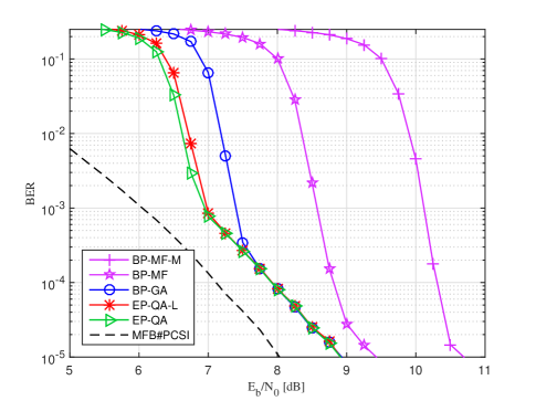
Refer to caption
Figure 7: BER versus Eb/N0subscript𝐸𝑏subscript𝑁0E_{b}/N_{0} in the 64×864864\times 8 MIMO system with 16QAM.
Refer to caption
Figure 8: BER versus Eb/N0subscript𝐸𝑏subscript𝑁0E_{b}/N_{0} in the 16×816816\times 8 MIMO system with 16QAM.
Refer to caption
(a) BP-MF-M.
Refer to caption
(b) BP-GA.
Refer to caption
(c) EP-QA-L.
Refer to caption
(d) EP-QA.
Figure 9: BER versus Eb/N0subscript𝐸𝑏subscript𝑁0E_{b}/N_{0} in the 64×864864\times 8 MIMO system with 16QAM.
Refer to caption
(a) BP-MF-M.
Refer to caption
(b) BP-MF.
Refer to caption
(c) BP-GA.
Refer to caption
(d) EP-QA.
Refer to caption
(e) EP-QA-L.
Figure 10: BER versus Eb/N0subscript𝐸𝑏subscript𝑁0E_{b}/N_{0} in the 16×816816\times 8 MIMO system with 16QAM.

V-B BER𝐵𝐸𝑅BER Versus Eb/N0subscript𝐸𝑏subscript𝑁0E_{b}/N_{0}

Fig. 7 and Fig. 8 show the BER performance versus Eb/N0subscript𝐸𝑏subscript𝑁0E_{b}/N_{0} in the 64×864864\times 8 MIMO system and the 16×816816\times 8 MIMO system, respectively. The BP-GA, the EP-QA, and the EP-QA-L achieve the same performance that is about 0.9dB0.9dB0.9\,\text{dB} away from the MFB-PCSI at BER=105BERsuperscript105\text{BER}=10^{-5}, but the BP-MF-M is about 2.0dB2.0dB2.0\,\text{dB} away from the MFB-PCSI in the 64×864864\times 8 MIMO system and 2.6dB2.6dB2.6\,\text{dB} away from the MFB-PCSI in the 16×816816\times 8 MIMO system. In the 16×816816\times 8 MIMO system, even the BP-MF with much higher complexity is still inferior to the EP-QA-L about 0.5dB0.5dB0.5\,\text{dB} at BER=105BERsuperscript105\text{BER}=10^{-5}.

Fig. 9 and Fig. 10 show the BER performance versus Eb/N0subscript𝐸𝑏subscript𝑁0E_{b}/N_{0} with increasing number of turbo iterations. In the 64×864864\times 8 MIMO system, to converge at BER=105BERsuperscript105\text{BER}=10^{-5}, the BP-GA, the EP-QA, and the EP-QA-L need about 7 turbo iterations and the BP-MF-M needs about 12 turbo iterations. In the 16×816816\times 8 MIMO system, the BP-GA, the EP-QA, and the EP-QA-L need 9 turbo iterations to converge at BER=105BERsuperscript105\text{BER}=10^{-5} and the BP-MF needs about 12 turbo iterations, while the performance of BP-MF-M is somewhat unstable.

VI Conclusion

In this paper, we presented a message-passing receiver for joint channel-estimation and decoding in the 3D massive MIMO systems transmitting over frequency-selective block fading channels. Expectation propagation with quadratic approximation was derived to deal with the decoupling of channel coefficients and data symbols, and a low-complexity Gaussian message-passing algorithm was applied for the channel estimation. It was verified through simulations that in the 3D massive MIMO systems our proposed algorithm could approach to the MFB with limited loss and its complexity is very low.

Acknowledgment

The authors would like to gratefully acknowledge Prof. P. Schniter for valuable suggestions, especially on the issue of negative variances occurred in the EP algorithm.

Using the so-called Wirtinger calculus [43, 44], a real function of z𝑧z\in\mathbb{C}, τ>0𝜏0\tau>0 and u𝑢u\in\mathbb{C} is defined by

(𝒛,τ,u)=|z|2τ+𝗅𝗇τ+|u|2ν,𝒛𝜏𝑢superscript𝑧2𝜏𝗅𝗇𝜏superscript𝑢2𝜈\mathcal{H}\left(\vec{\boldsymbol{z}},\tau,\vec{u}\right)=\frac{\left|z\right|^{2}}{\tau}+\mathsf{ln}\tau+\frac{\left|u\right|^{2}}{\nu}, (70)

where the conjugate coordinates 𝒛𝒛\vec{\boldsymbol{z}} and 𝒖𝒖\vec{\boldsymbol{u}} are defined by 𝒛[z,z]𝖳𝒛superscript𝑧superscript𝑧𝖳\vec{\boldsymbol{z}}\triangleq\left[z,z^{*}\right]^{\mathsf{T}} and 𝒖[u,u]𝖳𝒖superscript𝑢superscript𝑢𝖳\vec{\boldsymbol{u}}\triangleq\left[u,u^{*}\right]^{\mathsf{T}} respectively, and ν>0𝜈0\nu>0 is a constant. For the function (𝒛,τ,u)𝒛𝜏𝑢\mathcal{H}\left(\vec{\boldsymbol{z}},\tau,\vec{u}\right), some of its partial derivations are given by

𝒛𝒛\displaystyle\frac{\partial\mathcal{H}}{\partial\vec{\boldsymbol{z}}} [z,z]=[zτ,zτ],absent𝑧superscript𝑧superscript𝑧𝜏𝑧𝜏\displaystyle\triangleq\left[\frac{\partial\mathcal{H}}{\partial z},\frac{\partial\mathcal{H}}{\partial z^{*}}\right]=\left[\frac{z^{*}}{\tau},\frac{z}{\tau}\right], (71)
2𝒛𝒛superscript2𝒛𝒛\displaystyle\frac{\partial^{2}\mathcal{H}}{\partial\vec{\boldsymbol{z}}\partial\vec{\boldsymbol{z}}} [z(z)z(z)z(z)z(z)]=[1τ001τ],absentdelimited-[]𝑧superscript𝑧superscript𝑧superscript𝑧𝑧superscriptsuperscript𝑧superscript𝑧superscriptsuperscript𝑧delimited-[]1𝜏001𝜏\displaystyle\triangleq\left[\begin{array}[]{cc}\frac{\partial}{\partial z}\left(\frac{\partial\mathcal{H}}{\partial z}\right)^{*}&\frac{\partial}{\partial z^{*}}\left(\frac{\partial\mathcal{H}}{\partial z}\right)^{*}\\ \frac{\partial}{\partial z}\left(\frac{\partial\mathcal{H}}{\partial z^{*}}\right)^{*}&\frac{\partial}{\partial z^{*}}\left(\frac{\partial\mathcal{H}}{\partial z^{*}}\right)^{*}\end{array}\right]=\left[\begin{array}[]{cc}\frac{1}{\tau}&0\\ 0&\frac{1}{\tau}\end{array}\right], (76)
τ𝜏\displaystyle\frac{\partial\mathcal{H}}{\partial\tau} =1τ|z|2τ2,absent1𝜏superscript𝑧2superscript𝜏2\displaystyle=\frac{1}{\tau}-\frac{\left|z\right|^{2}}{\tau^{2}}, (77)
𝒖𝒖\displaystyle\frac{\partial\mathcal{H}}{\partial\vec{\boldsymbol{u}}} [u,u]=[uν,uν],\displaystyle\triangleq\left[\frac{\partial\mathcal{H}}{\partial u},\frac{\partial\mathcal{H}}{\partial u^{*}}\right]=\left[\frac{u*}{\nu},\frac{u}{\nu}\right], (78)
2𝒖𝒖superscript2𝒖𝒖\displaystyle\frac{\partial^{2}\mathcal{H}}{\partial\vec{\boldsymbol{u}}\partial\vec{\boldsymbol{u}}} [u(u)u(u)u(u)u(u)]=[1ν001ν].\displaystyle\triangleq\left[\begin{array}[]{cc}\frac{\partial}{\partial u}\left(\frac{\partial\mathcal{H}}{\partial u}\right)^{*}&\frac{\partial}{\partial u*}\left(\frac{\partial\mathcal{H}}{\partial u}\right)^{*}\\ \frac{\partial}{\partial u}\left(\frac{\partial\mathcal{H}}{\partial u^{*}}\right)^{*}&\frac{\partial}{\partial u^{*}}\left(\frac{\partial\mathcal{H}}{\partial u^{*}}\right)^{*}\end{array}\right]=\left[\begin{array}[]{cc}\frac{1}{\nu}&0\\ 0&\frac{1}{\nu}\end{array}\right]. (83)

Up to the second order, the power series expansion of (𝒛,τ,𝒖)𝒛𝜏𝒖\mathcal{H}\left(\vec{\boldsymbol{z}},\tau,\vec{\boldsymbol{u}}\right) at the point (𝒛0,τ0,𝒖0)subscript𝒛0subscript𝜏0subscript𝒖0\left(\vec{\boldsymbol{z}}_{0},\tau_{0},\vec{\boldsymbol{u}}_{0}\right) is given by [44]

(𝒛,τ,𝒖)𝒛𝜏𝒖\displaystyle\mathcal{H}\left(\vec{\boldsymbol{z}},\tau,\vec{\boldsymbol{u}}\right) (𝒛0,τ0,𝒖0)+𝒛0Δ𝒛+τ0Δτ+𝒖0Δ𝒖absentsubscript𝒛0subscript𝜏0subscript𝒖0subscript𝒛0Δ𝒛subscript𝜏0Δ𝜏subscript𝒖0Δ𝒖\displaystyle\approx\mathcal{H}\left(\vec{\boldsymbol{z}}_{0},\tau_{0},\vec{\boldsymbol{u}}_{0}\right)+\frac{\partial\mathcal{H}}{\partial\vec{\boldsymbol{z}}_{0}}\Delta\vec{\boldsymbol{z}}+\frac{\partial\mathcal{H}}{\partial\tau_{0}}\Delta\tau+\frac{\partial\mathcal{H}}{\partial\vec{\boldsymbol{u}}_{0}}\Delta\vec{\boldsymbol{u}}
+12(Δ𝒛)𝖧2𝒛0𝒛0Δ𝒛+12(Δ𝒖)𝖧2𝒖0𝒖0Δ𝒖12superscriptΔ𝒛𝖧superscript2subscript𝒛0subscript𝒛0Δ𝒛12superscriptΔ𝒖𝖧superscript2subscript𝒖0subscript𝒖0Δ𝒖\displaystyle\hskip 10.00002pt+\frac{1}{2}\left(\Delta\vec{\boldsymbol{z}}\right)^{\mathsf{H}}\frac{\partial^{2}\mathcal{H}}{\partial\vec{\boldsymbol{z}}_{0}\partial\vec{\boldsymbol{z}}_{0}}\Delta\vec{\boldsymbol{z}}+\frac{1}{2}\left(\Delta\vec{\boldsymbol{u}}\right)^{\mathsf{H}}\frac{\partial^{2}\mathcal{H}}{\partial\vec{\boldsymbol{u}}_{0}\partial\vec{\boldsymbol{u}}_{0}}\Delta\vec{\boldsymbol{u}}
=(𝒛0,τ0,𝒖0)+2{z0τ0Δz+u0νΔu}absentsubscript𝒛0subscript𝜏0subscript𝒖02superscriptsubscript𝑧0subscript𝜏0Δ𝑧superscriptsubscript𝑢0𝜈Δ𝑢\displaystyle=\mathcal{H}\left(\vec{\boldsymbol{z}}_{0},\tau_{0},\vec{\boldsymbol{u}}_{0}\right)+2\Re\left\{\frac{z_{0}^{*}}{\tau_{0}}\Delta z+\frac{u_{0}^{*}}{{}_{\nu}}\Delta u\right\}
|z0|2τ02Δτ+1τ0Δτ+1τ0|Δz|2+1ν|Δu|2,superscriptsubscript𝑧02superscriptsubscript𝜏02Δ𝜏1subscript𝜏0Δ𝜏1subscript𝜏0superscriptΔ𝑧21𝜈superscriptΔ𝑢2\displaystyle\hskip 10.00002pt-\frac{\left|z_{0}\right|^{2}}{\tau_{0}^{2}}\Delta\tau+\frac{1}{\tau_{0}}\Delta\tau+\frac{1}{\tau_{0}}\left|\Delta z\right|^{2}+\frac{1}{\nu}\left|\Delta u\right|^{2}, (84)

where Δ𝒛𝒛𝒛0Δ𝒛𝒛subscript𝒛0\Delta\vec{\boldsymbol{z}}\triangleq\vec{\boldsymbol{z}}-\vec{\boldsymbol{z}}_{0}, Δτττ0Δ𝜏𝜏subscript𝜏0\Delta\tau\triangleq\tau-\tau_{0} and Δ𝒖𝒖𝒖0Δ𝒖𝒖subscript𝒖0\Delta\vec{\boldsymbol{u}}\triangleq\vec{\boldsymbol{u}}-\vec{\boldsymbol{u}}_{0}

References

  • [1] T. L. Marzetta, “Noncooperative cellular wireless with unlimited numbers of base station antennas,” IEEE Trans. Wireless Commun., vol. 9, no. 11, pp. 3590–3600, Nov. 2010.
  • [2] F. Rusek, D. Persson, B. K. Lau, E. G. Larsson, T. L. Marzetta, O. Edfors, and F. Tufvesson, “Scaling up MIMO: Opportunities and challenges with very large arrays,” IEEE Signal Process. Mag., vol. 30, no. 1, pp. 40–60, Jan. 2013.
  • [3] J. Hoydis, S. ten Brink, and M. Debbah, “Massive MIMO in the UL/DL of cellular networks: How many antennas do we need?” IEEE J. Sel. Areas Commun., vol. 31, no. 2, pp. 160–171, Feb. 2013.
  • [4] E. G. Larsson, O. Edfors, F. Tufvesson, and T. L. Marzetta, “Massive MIMO for next generation wireless systems,” IEEE Communications Magazine, vol. 52, no. 2, pp. 186–195, February 2014.
  • [5] N. Shariati, E. Björnson, M. Bengtsson, and M. Debbah, “Low-complexity polynomial channel estimation in large-scale MIMO with arbitrary statistics,” IEEE J. Sel. Topics in Signal Process., vol. 8, no. 5, pp. 815–830, Oct. 2014.
  • [6] S. Noh, M. D. Zoltowski, Y. Sung, and D. J. Love, “Pilot beam pattern design for channel estimation in massive MIMO systems,” IEEE J. Sel. Topics in Signal Process., vol. 8, no. 5, pp. 787–801, Oct. 2014.
  • [7] P. S. Rossi and R. R. Müller, “Joint twofold-iterative channel estimation and multiuser detection for MIMO-OFDM systems,” IEEE Trans. Wireless Commun., vol. 7, no. 11, pp. 4719–4729, Nov. 2008.
  • [8] C. Novak, G. Matz, and F. Hlawatsch, “IDMA for the multiuser MIMO-OFDM uplink: A factor graph framework for joint data detection and channel estimation,” IEEE Trans. Signal Process., vol. 61, no. 16, pp. 4051–4066, Aug. 2013.
  • [9] Y. Liu, Z. Tan, H. Hu, L. J. Cimini, and G. Y. Li, “Channel estimation for OFDM,” IEEE Communications Surveys & Tutorials, vol. 16, no. 4, pp. 1891–1908, Fourth Quarter 2014.
  • [10] P. Zhang, S. Chen, and L. Hanzo, “Embedded iterative semi-blind channel estimation for three-stage-concatenated MIMO-aided QAM turbo transceivers,” IEEE Trans. Veh. Technol., vol. 63, no. 1, pp. 439–446, Jan. 2014.
  • [11] J. Ma and P. Li, “Data-aided channel estimation in large antenna systems,” IEEE Trans. Signal Process., vol. 62, no. 12, pp. 3111–3124, June 2014.
  • [12] S. Park, B. Shim, and J. W. Choi, “Iterative channel estimation using virtual pilot signals for MIMO-OFDM systems,” IEEE Trans. Signal Process., vol. 63, no. 12, pp. 3032–3045, June 2015.
  • [13] F. R. Kschischang, B. J. Frey, and H.-A. Loeliger, “Factor graphs and the sum-product algorithm,” IEEE Trans. Inf. Theory, vol. 47, no. 2, pp. 498–519, Feb. 2001.
  • [14] A. P. Worthen and W. E. Stark, “Unified design of iterative receivers using factor graphs,” IEEE Trans. Inf. Theory, vol. 47, no. 2, pp. 843–849, 2001.
  • [15] H. Wymeersch, Iterative Receiver Design.   Cambridge, U.K.: Cambridge Univ. Press, 2007.
  • [16] Y. Liu, L. Brunel, and J. J. Boutros, “Joint channel estimation and decoding using Gaussian approximation in a factor graph over multipath channel,” in Proc. Int. Symp. on Personal, Indoor and Mobile Radio Commun. (PIMRC), 2009, pp. 3164–3168.
  • [17] G. E. Kirkelund, C. N. Manchón, L. P. B. Christensen, E. Riegler, and B. H. Fleury, “Variational message-passing for joint channel estimation and decoding in MIMO-OFDM,” in Proc. IEEE Global Telecomm. Conf. (GLOBECOM ), 2010, pp. 1–6.
  • [18] C. N. Manchón, G. E. Kirkelund, E. Riegler, L. P. B. Christensen, and B. H. Fleury, “Receiver architectures for MIMO-OFDM based on a combined VMP-SP algorithm,” arXiv: 1111.5848, 2011.
  • [19] Q. Guo and D. D. Huang, “EM-based joint channel estimation and detection for frequency selective channels using gaussian message passing,” IEEE Trans. Signal Process., vol. 59, no. 8, pp. 4030–4035, 2011.
  • [20] P. Schniter, “A message-passing receiver for BICM-OFDM over unknown clustered-sparse channels,” IEEE J. Sel. Topics in Signal Process., vol. 5, no. 8, pp. 1462–1474, 2011.
  • [21] C. Knievel, P. A. Hoeher, A. Tyrrell, and G. Auer, “Multi-dimensional graph-based soft iterative receiver for MIMO-OFDM,” IEEE Trans. Commun., vol. 60, no. 6, pp. 1599–1609, June 2012.
  • [22] E. Riegler, G. E. Kirkelund, C. N. Manchón, M.-A. Badiu, and B. H. Fleury, “Merging belief propagation and the mean field approximation: A free energy approach,” IEEE Trans. Inf. Theory, vol. 59, no. 1, pp. 588–602, Jan. 2013.
  • [23] X. Zhang, P. Xiao, D. Ma, and J. Wei, “Variational-bayes-assisted joint signal detection, noise covariance estimation, and channel tracking in MIMO-OFDM systems,” IEEE Trans. Veh. Technol., vol. 63, no. 9, pp. 4436–4449, Nov. 2014.
  • [24] D. D. Lin and T. J. Lim, “A variational inference framework for soft-in soft-out detection in multiple-access channels,” IEEE Trans. Inf. Theory, vol. 55, no. 5, pp. 2345–2364, May 2009.
  • [25] P. Schniter, “Joint estimation and decoding for sparse channels via relaxed belief propagation,” in Proc. of 44th Asilomar Conference on Signals, Systems and Computers. (ASILOMAR).   IEEE, 2010, pp. 1055–1059.
  • [26] M.-A. Badiu, G. E. Kirkelund, C. N. Manchón, E. Riegler, and B. H. Fleury, “Message-passing algorithms for channel estimation and decoding using approximate inference,” in Proc. IEEE Int. Symp. Inf. Theory (ISIT), 2012, pp. 2376–2380.
  • [27] A. Drémeau, C. Herzet, and L. Daudet, “Boltzmann machine and mean-field approximation for structured sparse decompositions,” IEEE Trans. Signal Process., vol. 60, no. 7, pp. 3425–3438, July 2012.
  • [28] F. Krzakala, A. Manoel, E. Tramel, and L. Zdeborová, “Variational free energies for compressed sensing,” in Proc. IEEE International Symposium on Information Theory (ISIT), June 2014, pp. 1499–1503.
  • [29] M.-A. Badiu, C. Manchón, and B. Fleury, “Message-passing receiver architecture with reduced-complexity channel estimation,” IEEE Commun. Lett., vol. 17, no. 7, pp. 1404–1407, Jul. 2013.
  • [30] T. P. Minka, “A family of algorithms for approximate Bayesian inference,” Ph.D. dissertation, Massachusetts Institute of Technology, 2001.
  • [31] S. Wu, L. Kuang, Z. Ni, J. Lu, D. D. Huang, and Q. Guo, “Expectation propagation approach to joint channel estimation and decoding for OFDM systems,” in Proc. IEEE Int. Conf. on Acoust., Speech and Signal Process. (ICASSP), Florence, Italy, May 2014, pp. 1941–1945.
  • [32] J. T. Parker, P. Schniter, and V. Cevher, “Bilinear generalized approximate message passing–Part I: Derivation,” IEEE Trans. Signal Process., vol. 62, no. 22, pp. 5839–5853, Nov. 2014.
  • [33] L. Schumacher, K. Pedersen, and P. Mogensen, “From antenna spacings to theoretical capacities-guidelines for simulating MIMO systems,” in Proc. IEEE Int. Symp. PIMRC, 2002, pp. 587–592.
  • [34] D. Ying, F. W. Vook, T. A. Thomas, D. J. Love, and A. Ghosh, “Kronecker product correlation model and limited feedback codebook design in a 3D channel model,” in Proc. of 2014 IEEE International Conference on Communications (ICC), Jun. 2014, pp. 5865–5870.
  • [35] L. Dai, Z. Wang, and Z. Yang, “Spectrally efficient time-frequency training OFDM for mobile large-scale MIMO systems,” IEEE J. Sel. Areas Commun., vol. 3, no. 2, pp. 251–263, Feb. 2013.
  • [36] P. Som, T. Datta, N. Srinidhi, A. Chockalingam, and B. Rajan, “Low-complexity detection in large-dimension MIMO-ISI channels using graphical models,” IEEE J. Sel. Topics in Signal Process., vol. 5, no. 8, pp. 1497–1511, Dec. 2011.
  • [37] C. M. Bishop et al., Pattern recognition and machine learning.   New York: Springer, 2006.
  • [38] J. Hu, H.-A. Loeliger, J. Dauwels, and F. Kschischang, “A general computation rule for lossy summaries/messages with examples from equalization,” in Proc. 44th Allerton Conf. Communication, Control, and Computing, 2006, pp. 27–29.
  • [39] M. R. Andersen, A. Vehtari, O. Winther, and L. K. Hansen, “Bayesian inference for spatio-temporal spike and slab priors,” arXiv:1509.04752, 2015.
  • [40] D. Hernández-Lobato, J. M. Hernández-Lobato, and P. Dupont, “Generalized spike-and-slab priors for Bayesian group feature selection using expectation propagation,” The Journal of Machine Learning Research, vol. 14, no. 1, pp. 1891–1945, 2013.
  • [41] J. M. Winn and C. M. Bishop, “Variational message passing,” The Journal of Machine Learning Research, vol. 6, pp. 661–694, 2005.
  • [42] B. M. Hochwald and S. ten Brink, “Achieving near-capacity on a multiple-antenna channel,” IEEE Trans. Commun., vol. 51, no. 3, pp. 389–399, Mar. 2003.
  • [43] A. Van Den Bos, “Complex gradient and Hessian,” in IEE Proc. Vis., Image and Signal Processing, vol. 141, no. 6.   IET, 1994, pp. 380–383.
  • [44] K. Kreutz-Delgado, “The complex gradient operator and the CR-calculus,” arXiv preprint arXiv:0906.4835, 2009.