Multilevel quadrature for elliptic parametric partial differential equations in case of polygonal approximations of curved domains

Abstract.

Multilevel quadrature methods for parametric operator equations such as the multilevel (quasi-) Monte Carlo method are closely related to the sparse tensor product approximation between the spatial variable and the parameter. In this article, we employ this fact and reverse the multilevel quadrature method via the sparse grid construction by applying differences of quadrature rules to finite element discretizations of increasing resolution. Besides being algorithmically more efficient if the underlying quadrature rules are nested, this way of performing the sparse tensor product approximation enables the easy use of non-nested and even adaptively refined finite element meshes. Especially, we present a rigorous error and regularity analysis of the fully discrete solution, taking into account the effect of polygonal approximations to a curved physical domain and the numerical approximation of the bilinear form. Our results facilitate the construction of efficient multilevel quadrature methods based on deterministic quadrature rules. Numerical results in three spatial dimensions are provided to illustrate the approach.

1. Introduction

The present article is concerned with the numerical solution of elliptic parametric second order boundary value problems of the form

(1) $$-\operatorname{div}\big{(}a({{\bm{y}}})\nabla u({{\bm{y}}})\big{)}=f({{\bm{y}}})\text{ in }D,\quad u({{\bm{y}}})=0\text{ on }\partial D,\quad{{\bm{y}}}\in{{\Gamma}},$$

where $D\subset\mathbb{R}^{d}$ denotes the spatial domain and ${{\Gamma}}\subset\mathbb{R}^{m}$ denotes the parameter domain. Prominent representatives of such problems arise from recasting boundary value problems with random data, like random diffusion coefficients, random right hand sides and even random domains. A high-dimensional parametric boundary value problem of the form (1) is then derived by inserting the truncated Karhunen-Loève expansion of the random data, see e.g.  [1, 2, 12, 24, 33]. Hence, the computation of quantities of interest amounts to a high-dimensional Bochner integration problem. The latter can be dealt with by quadrature methods. Since every quadrature method requires the repeated evaluation of the integrand for different sample or quadrature points, we have to compute the solution to (1) with respect to many different values of the parameter ${{\bm{y}}}\in{{\Gamma}}$.

An efficient approach to deal with the quadrature problem is the multilevel Monte Carlo method (MLMC), which has been developed in [3, 16, 18, 27, 28]. As first observed in [14, 22], this approach mimics a certain sparse grid approximation between the physical space and the parameter space. Thus, the extension to the multilevel quasi-Monte Carlo (MLQMC) method and even more general multilevel quadrature methods is obvious. In this article, we focus on such deterministic quadrature methods, which, in particular, require extra regularity of the solution in terms of spaces of dominant mixed derivatives, cf. [22, 25, 31] for example. This extra regularity is available for important classes of parametric problems, see [9, 10] for the case of affine elliptic diffusion coefficients and [30] for the case of log-normally distributed diffusion coefficients. For the sake of clarity in presentation, we shall focus here on affine elliptic diffusion problems as they occur from the discretization of uniformly elliptic random diffusion coefficients. We put our emphasis on the rigorous error and regularity analysis of the fully discrete solution, taking into account the effect of polygonal approximations to a curved physical domain and the numerical approximation of the bilinear form.

In addition, we focus on a particular construction of the multilevel quadrature, which is very well suited for the use with black-box finite element solvers and adaptive mesh refinements: Taking the fact that a multilevel quadrature scheme resembles a sparse tensor product approximation between the spatial variable and the parametric variable as a starting point, we have the following abstract framework. Let

$$V_{0}^{(i)}\subset V_{1}^{(i)}\subset\cdots\subset V_{j}^{(i)}\subset\cdots\subset\mathcal{H}_{i},\quad i=1,2,$$

denote two sequences of finite dimensional sub-spaces with increasing approximation power in some linear spaces $\mathcal{H}_{i}$. To approximate a given object of the tensor product space $\mathcal{H}_{1}\otimes\mathcal{H}_{2}$, one canonically considers the full tensor product spaces $U_{j}\mathrel{\mathrel{\mathop{:}}=}V_{j}^{(1)}\otimes V_{j}^{(2)}$. However, the cost $\dim U_{j}=\dim V_{j}^{(1)}\cdot\dim V_{j}^{(2)}$ is often too expensive. To reduce this cost, one might consider the approximation in so-called sparse grid spaces, see e.g. [7]. For $\ell\geq 0$, one introduces the complement spaces

$$W_{\ell+1}^{(i)}=V_{\ell+1}^{(i)}\ominus V_{\ell}^{(i)},\quad i=1,2,$$

which gives rise to the multilevel decompositions

(2) $$V_{j}^{(i)}=\bigoplus_{\ell=0}^{j}W_{\ell}^{(i)},\quad W_{0}^{(i)}:=V_{0}^{(i)},\quad i=1,2.$$

Then, the sparse grid space is defined by

(3) $$\widehat{U}_{j}:=\bigoplus_{\ell+\ell^{\prime}\leq j}W_{\ell}^{(1)}\otimes W_{\ell^{\prime}}^{(2)}.$$

Under the assumptions that the dimensions of $\big{\{}V_{\ell}^{(1)}\big{\}}$ and $\big{\{}V_{\ell}^{(2)}\big{\}}$ form geometric series, (3) contains, at most up to a logarithm, only $\mathcal{O}\big{(}\max\big{\{}\dim V_{j}^{(1)},\dim V_{j}^{(2)}\big{\}}\big{)}$ degrees of freedom. Nevertheless, it offers nearly the same approximation power as $U_{j}$ provided that the object to be approximated has some extra smoothness by means of mixed regularity. For further details, see [19].

Figure 1. Different representations of the sparse grid space.

In view of (2), factoring out with respect to the first component, one can rewrite (3) according to

(4) $$\widehat{U}_{j}=\bigoplus_{\ell=0}^{j}W_{\ell}^{(1)}\otimes\bigg{(}\bigoplus_{\ell^{\prime}=0}^{j-\ell}W_{\ell^{\prime}}^{(2)}\bigg{)}=\bigoplus_{\ell=0}^{j}W_{\ell}^{(1)}\otimes V_{j-\ell}^{(2)}.$$

This representation has already been proposed in [19]. Obviously, in complete analogy there holds

(5) $$\widehat{U}_{j}=\bigoplus_{\ell^{\prime}=0}^{j}\bigg{(}\bigoplus_{\ell=0}^{j-\ell^{\prime}}W_{\ell}^{(1)}\bigg{)}\otimes W_{\ell^{\prime}}^{(2)}=\bigoplus_{\ell=0}^{j}V_{j-\ell}^{(1)}\otimes W_{\ell}^{(2)}.$$

We refer to Fig. 1 for an illustration, where the left plot corresponds to the representation (4) and the right plot corresponds to the representation (5). The advantage of the representation (4) is that we can give up the requirement that the spaces $\{V_{\ell}^{(2)}\}$ are nested. Likewise, for the representation (5), the spaces $\{V_{\ell}^{(1)}\}$ need not to be nested any more.

In the context of the parametric diffusion problem (1), we aim at computing

$$\int_{{\Gamma}}\mathcal{F}\big{(}u({{\bm{y}}})\big{)}\rho({{\bm{y}}})\operatorname{d}\!{{\bm{y}}},$$

where $\rho$ is the density of some measure on $\Gamma$ and $\mathcal{F}$ denotes a functional or, as in the case of moment computation, it may be defined as $\mathcal{F}\big{(}u({{\bm{y}}})\big{)}=u^{p}({{\bm{y}}})$ for $p=1,2,\ldots$. In this context, $\{V_{\ell}^{(1)}\}$ corresponds to a sequence of finite element spaces and $\{V_{\ell}^{(2)}\}$ refers to a sequence of quadrature rules. If we denote the finite element solutions of (1) by $\mathfrak{u}_{\ell}({{\bm{y}}})\in V_{\ell}^{(1)}$ and if we denote the sequence of quadrature rules by $Q_{\ell^{\prime}}\colon C({{\Gamma}})\to\mathbb{R}$, we thus arrive with respect to (4) at the decomposition

(6) $$\int_{{\Gamma}}\mathcal{F}\big{(}u({{\bm{y}}})\big{)}\rho({{\bm{y}}})\operatorname{d}\!{{\bm{y}}}\approx\sum_{\ell=0}^{j}Q_{j-\ell}\Delta\mathcal{F}_{\ell}\big{(}u({{\bm{y}}})\big{)},$$

where $\Delta\mathcal{F}_{\ell}\big{(}u({{\bm{y}}})\big{)}\mathrel{\mathrel{\mathop{:}}=}\mathcal{F}\big{(}\mathfrak{u}_{\ell}({{\bm{y}}})\big{)}-\mathcal{F}\big{(}\mathfrak{u}_{\ell-1}({{\bm{y}}})\big{)}$ and $\mathcal{F}\big{(}\mathfrak{u}_{-1}({{\bm{y}}})\big{)}\mathrel{\mathrel{\mathop{:}}=}0$, see [22]. On the other hand, similarly to (5), we obtain the decomposition

(7) $$\int_{{\Gamma}}\mathcal{F}\big{(}u({{\bm{y}}})\big{)}\rho({{\bm{y}}})\operatorname{d}\!{{\bm{y}}}\approx\sum_{\ell=0}^{j}\Delta Q_{\ell}\mathcal{F}\big{(}\mathfrak{u}_{j-\ell}({{\bm{y}}})\big{)},$$

where $\Delta Q_{\ell}\mathrel{\mathrel{\mathop{:}}=}Q_{\ell}-Q_{\ell-1}$ and $Q_{-1}\mathrel{\mathrel{\mathop{:}}=}0$. Both representations are equivalent but have a different impact on its numerical implementation.

Originally, multilevel quadrature methods have been interpreted as variance reduction methods for the Monte Carlo quadrature, a view which has originally been introduced for the approximation of parametric integrals, cf. [27, 28]. Consequently, the representation (4), and thus the decomposition (6), has been used in previous articles, see, for example, [16, 17] for stochastic ordinary differential equations and [3, 22, 38, 39] for partial differential equations with random data. To this end, usually a nested sequence of approximation spaces is presumed such that the complement spaces $\big{\{}W_{\ell}^{(1)}\big{\}}$ are well-defined. In the context of partial differential equations, these complement spaces are given via the difference of Galerkin projections onto subsequent finite element spaces. This circumstance can be avoided in the case of $\mathcal{F}$ being a functional, cf. [20, 38]. Still, we emphasize that, particularly in the context of the Monte Carlo method, there are already results available, which allow for giving up this nestedness, see e.g. [8, 38]. A more general result addressing the resulting error in the underlying bilinear form can be found in [37].

The decomposition (6) is well suited if the spatial dimension is small, as it is the case for one-dimensional partial differential equations with random data or for stochastic ordinary differential equations. Nevertheless, in two or three spatial dimensions, the construction of nested approximation spaces might be difficult or even not be possible at all. Sometimes, in view of adaptive refinement strategies, it might be favourable to give up nestedness. In the article at hand, we employ the decomposition (7). It allows more naturally for non-nested finite element spaces which, in turn, induce different approximations of the underlying domain. Moreover, using nested quadrature formulae, a considerable speed-up is achieved in comparison to the conventional multilevel quadrature which is based on the representation (6).

The rest of the article is organized as follows. We start by introducing the underlying random model in Section 2 and perform the parametric reformulation that results in (1). Then, the next two sections are dedicated to the discretization, namely the quadrature rule for the parametric variable (Section 3) and the finite element discretization for the physical domain (Section 4). The multilevel quadrature for the model problem is discussed in Section 5. In Section 6, we present the error and regularity analysis for the multilevel quadrature taking into account polygonal approximations of curved domains. We emphasize that the key result in this section, namely Lemma 6.1, is robust with respect to the parameter dimension $m$. Afterwards, in Section 7, we consider a fully discrete approximation of the solution to (1) and take also quadrature errors in the bilinear form into account. Again, the main result (Theorem 7.2) is robust with respect to the parameter dimension $m$. Finally, in Section 8, we provide numerical results in three spatial dimensions to validate our approach.

Throughout this article, in order to avoid the repeated use of generic but unspecified constants, we mean by $C\lesssim D$ that $C$ can be bounded by a multiple of $D$, independently of parameters which $C$ and $D$ may depend on. Obviously, $C\gtrsim D$ is defined as $D\lesssim C$, and $C\sim D$ as $C\lesssim D$ and $C\gtrsim D$.

2. Problem setting

Let $(\Omega,\Sigma,\mathbb{P})$ be a complete and separable probability space with $\sigma$-field $\Sigma\subset 2^{\Omega}$ and probability measure $\mathbb{P}$. We intend to compute the expectation

$$\mathbb{E}[u]=\int_{\Omega}u(\omega)\operatorname{d}\!\mathbb{P}(\omega)\in H_{0}^{1}(D)$$

and the variance

$$\mathbb{V}[u]=\int_{\Omega}\big{\{}u(\omega)-\mathbb{E}[u]\big{\}}^{2}\operatorname{d}\!\mathbb{P}(\omega)\in W_{0}^{1,1}(D)$$

of the random function $u(\omega)\in H_{0}^{1}(D)$ which solves the stochastic diffusion problem

(8) $$-\operatorname{div}\big{(}{{a}}(\omega)\nabla u(\omega)\big{)}=f\ \text{in}\ D\ \text{for almost every $\omega\in\Omega$}.$$

For sake of simplicity, we assume that the stochastic diffusion coefficient is given by a finite Karhunen-Loève expansion

(9) $${{a}}({{\bm{x}}},\omega)=\mathbb{E}[{{a}}]({{\bm{x}}})+\sum_{k=1}^{m}\sqrt{\lambda_{k}}\varphi_{k}({{\bm{x}}})\psi_{k}(\omega)$$

with pairwise $L^{2}$-orthonormal functions $\varphi_{k}\in L^{\infty}(D)$ and stochastically independent random variables $\psi_{k}(\omega)\in[-1,1]$. Especially, it is assumed that the random variables admit continuous density functions $\rho_{k}\colon[-1,1]\to\mathbb{R}$ with respect to the Lebesgue measure.

In practice, one generally has to compute the expansion (9) from the given covariance kernel

$$\operatorname{Cov}[{{a}}]({{\bm{x}}},{{\bm{x}}}^{\prime})=\int_{\Omega}\big{\{}{{a}}({{\bm{x}}},\omega)-\mathbb{E}[{{a}}]({{\bm{x}}})\big{\}}\big{\{}{{a}}({{\bm{x}}}^{\prime},\omega)-\mathbb{E}[{{a}}]({{\bm{x}}}^{\prime})\big{\}}\operatorname{d}\!\mathbb{P}(\omega).$$

If the expansion contains infinitely many terms, it has to be appropriately truncated which will induce an additional discretization error. For details, we refer the reader to [15, 23, 32, 36].

The assumption that the random variables $\{\psi_{k}(\omega)\}$ are independent implies that the joint density function of the random variables is given by ${\rho}({{\bm{y}}})\mathrel{\mathrel{\mathop{:}}=}\prod_{k=1}^{m}\rho_{k}(y_{k}).$

Thus, we are able to reformulate the stochastic problem (8) as a parametric, deterministic problem in $L^{2}_{{\rho}}({{\Gamma}})$. To this end, the probability space $\Omega$ is identified with its image ${{\Gamma}}\mathrel{\mathrel{\mathop{:}}=}[-1,1]^{m}$ with respect to the measurable mapping

$$\bm{\psi}\colon\Omega\to{{\Gamma}},\quad\omega\mapsto\bm{\psi}(\omega)\mathrel{\mathrel{\mathop{:}}=}\big{(}\psi_{1}(\omega),\ldots,\psi_{m}(\omega)\big{)}.$$

Hence, the random variables $\psi_{k}$ are substituted by coordinates $y_{k}\in[-1,1]$.

We introduce the measure ${\rho}({\bm{y}})\operatorname{d}\!{{\bm{y}}}$ on ${{\Gamma}}$, which is defined by the product density function ${\rho}({{\bm{y}}})\mathrel{\mathrel{\mathop{:}}=}\prod_{k=1}^{m}\rho_{k}(y_{k}).$

Next, in order to ensure $H^{2}$-regularity of the model problem, let $D\subset\mathbb{R}^{d}$, $d=2,3$, be either a convex, polygonal domain. We consider the parametric diffusion problem

(10) find $$u\in{L^{2}_{{\rho}}\big{(}{{\Gamma}};H_{0}^{1}(D)\big{)}}$$ such that

$$\qquad-\operatorname{div}\big{(}{{a}}({{\bm{y}}})\nabla u({{\bm{y}}})\big{)}=f\ \text{in $D$}\ \text{for almost every ${{\bm{y}}}\in{{\Gamma}}$},$$

with $f\in L^{2}(D)$ and ${{a}}\colon D\times{{\Gamma}}\to\mathbb{R}$ with

(11) $${{a}}({{\bm{x}}},{{\bm{y}}})=\varphi_{0}({{\bm{x}}})+\sum_{k=1}^{m}\sqrt{\lambda_{k}}\varphi_{k}({{\bm{x}}})y_{k},\quad\gamma_{k}\mathrel{\mathrel{\mathop{:}}=}\sqrt{\lambda_{k}}\|\varphi_{k}\|_{W^{1,\infty}(D)}.$$

Note that $u\in L^{2}_{{\rho}}\big{(}{{\Gamma}};H_{0}^{1}(D)\big{)}$ guarantees finite second order moments of the solution.

By the Lax-Milgram theorem, the unique solvability of the parametric diffusion problem (10) in $L_{\rho}^{2}\big{(}{{\Gamma}};H_{0}^{1}(D)\big{)}$ follows immediately if we impose the condition

(12) $$0<{{a}}_{\min}\leq{{a}}({{\bm{y}}})\leq{{a}}_{\max}<\infty\ \text{in $D$}$$

for all ${{\bm{y}}}\in{{\Gamma}}$ on the diffusion coefficient. Moreover, we obtain the stability estimate

$$\|u({{\bm{y}}})\|_{H^{1}(D)}\leq\frac{1}{a_{\min}}\|f\|_{H^{-1}(D)}\lesssim\frac{1}{a_{\min}}\|f\|_{L^{2}(D)}\quad\text{for almost every }{{\bm{y}}}\in{{\Gamma}}.$$

Hence, the solution to (10) is essentially bounded with respect to ${{\bm{y}}}\in{{\Gamma}}$.

In e.g. [4, 9, 10, 11, 40], it has been proven that the solution $u$ of (10) is analytical as mapping $u\colon{{\Gamma}}\to H_{0}^{1}(D)$. Moreover, it has been shown in [9] that $u$ is even an analytical mapping $u\colon{{\Gamma}}\to\mathcal{W}\mathrel{\mathrel{\mathop{:}}=}H_{0}^{1}(D)\cap H^{2}(D)$ given that the $\{\varphi_{k}\}$ in (11) belong to $W^{1,\infty}(D)$. This constitutes the necessary mixed regularity for a sparse tensor product discretization, see e.g. [25, 31]. A similar result for diffusion problems with coefficients of the form $\exp\big{(}{{a}}({{\bm{x}}},{{\bm{y}}})\big{)}$ has been shown in [30].

Since $u$ is supposed to be in $L^{2}_{{\rho}}\big{(}{{\Gamma}};H_{0}^{1}(D)\big{)}$, we can compute its expectation

(13) $$\mathbb{E}[u]=\int_{{{\Gamma}}}u({{\bm{y}}}){\rho}({{\bm{y}}})\operatorname{d}\!{{\bm{y}}}\in H_{0}^{1}(D)$$

and its variance

(14) $$\mathbb{V}[u]=\mathbb{E}[u^{2}]-\mathbb{E}[u]^{2}=\int_{{\Gamma}}u^{2}({{\bm{y}}}){\rho}({{\bm{y}}})\operatorname{d}\!{{\bm{y}}}-\mathbb{E}[u]^{2}\in W_{0}^{1,1}(D).$$

We will focus in the sequel on the efficient numerical computation of these possibly high-dimensional integrals.

3. Quadrature in the parameter space

The expectation and the variance of the solution $u$ to (10) are given by the integrals (13) and (14). To compute these integrals, we employ a sequence of quadrature formulae $\{Q_{\ell}\}$ for the Bochner integral

$$\operatorname{Int}\colon L_{\rho}^{1}({{\Gamma}};\mathcal{X})\to\mathcal{X},\quad\operatorname{Int}v=\int_{{\Gamma}}v({{\bm{y}}})\rho({{\bm{y}}})\operatorname{d}\!{{\bm{y}}}$$

where $\mathcal{X}\subset L^{2}(D)$ denotes some Banach space. The quadrature formula

(15) $$Q_{\ell}\colon L_{\rho}^{1}({{\Gamma}};\mathcal{X})\to\mathcal{X},\quad(Q_{\ell}v)({{\bm{x}}})=\sum_{i=1}^{N_{\ell}}\omega_{\ell,i}v({{\bm{x}}},\bm{\xi}_{\ell,i})\rho(\bm{\xi}_{\ell,i})$$

is supposed to provide the error bound

(16) $$\|(\operatorname{Int}-Q_{\ell})v\|_{\mathcal{X}}\lesssim\varepsilon_{\ell}\|v\|_{\mathcal{H}({{\Gamma}};\mathcal{X})}$$

uniformly in $\ell\in\mathbb{N}$, where $\mathcal{H}({{\Gamma}};\mathcal{X})\subset L_{\rho}^{2}({{\Gamma}},\mathcal{X})$ is a suitable Bochner space. Note that since the density $\rho$ is fixed, it will be suppressed in the upcoming error estimates and will, thus, be hidden in the constants.

The following particular examples of quadrature rules (15) are considered in our numerical experiments:

• The Monte Carlo method satisfies (16) only with respect to the root mean square error. Namely, it holds

  $$\sqrt{\mathbb{E}\big{(}\|(\operatorname{Int}-Q_{\ell})v\|_{\mathcal{X}}^{2}\big{)}}\lesssim\varepsilon_{\ell}\|v\|_{\mathcal{H}({{\Gamma}};\mathcal{X})}$$

  with $\varepsilon_{\ell}=N_{\ell}^{-1/2}$ and $\mathcal{H}({{\Gamma}};\mathcal{X})=L_{\rho}^{2}({{\Gamma}};\mathcal{X})$.

• The quasi-Monte Carlo method leads typically to $\varepsilon_{\ell}=N_{\ell}^{-1}(\log N_{\ell})^{m}$, where it is sufficient to consider the Bochner space $\mathcal{H}({{\Gamma}};\mathcal{X})=W_{\text{mix}}^{1,1}({{\Gamma}};\mathcal{X})$ of all equivalence classes of functions $v\colon{{\Gamma}}\to\mathcal{X}$ with finite norm

  (17) $$\|v\|_{W_{\text{mix}}^{1,1}({{\Gamma}};\mathcal{X})}\mathrel{\mathrel{\mathop{:}}=}\sum_{\|{{\bm{q}}}\|_{\infty}\leq 1}\int_{{\Gamma}}\bigg{\|}\frac{\partial^{\|{{\bm{q}}}\|_{1}}}{\partial y_{1}^{q_{1}}\partial y_{2}^{q_{2}}\cdots\partial y_{m}^{q_{m}}}v({{\bm{y}}})\bigg{\|}_{\mathcal{X}}\operatorname{d}\!{{\bm{y}}}<\infty,$$

  see e.g. [34]. Note that, in this case, the estimate requires that the densities satisfy $\rho_{k}\in W^{1,\infty}(-1,1)$. For the Halton sequence, cf. [21], it can even be shown that $\varepsilon_{\ell}=N_{\ell}^{\delta-1}$ for arbitrary $\delta>0$ given that the spatial functions in (11) satisfy $\gamma_{k}\lesssim k^{-3-\varepsilon}$ for arbitrary $\varepsilon>0$. This is a straightforward consequence from the results in [41], see e.g. [24].

• Let the densities $\rho_{k}$ be in $W^{r,\infty}(-1,1)$. If $v\colon{{\Gamma}}\to\mathcal{X}$ has mixed regularity of order $r$ with respect to the parameter ${{\bm{y}}}$, i.e.

  (18) $$\|v\|_{W_{\text{mix}}^{r,\infty}({{\Gamma}};\mathcal{X})}\mathrel{\mathrel{\mathop{:}}=}\max_{\|{\bm{{\alpha}}}\|_{\infty}\leq r}\big{\|}\partial^{\bm{{\alpha}}}_{{\bm{y}}}v\big{\|}_{L^{\infty}({{\Gamma}};\mathcal{X})}<\infty,$$

  then one can apply a (sparse) tensor product Clenshaw-Curtis quadrature rule. This yields the convergence rate $\varepsilon_{\ell}=2^{-\ell r}\ell^{m-1}$, where $N_{\ell}\sim 2^{\ell}\ell^{m-1}$ and $\mathcal{H}({{\Gamma}};\mathcal{X})=W_{\text{mix}}^{r,\infty}({{\Gamma}};\mathcal{X})$, see [35].

For our purposes, we shall assume that the number $N_{\ell}$ of points of the quadrature formula ${Q}_{\ell}$ is chosen such that the corresponding accuracy is

(19) $$\varepsilon_{\ell}=2^{-\ell}.$$

Then, for the respective difference quadrature $\Delta Q_{\ell}\mathrel{\mathrel{\mathop{:}}=}Q_{\ell}-Q_{\ell-1}$, we immediately obtain by combining (16) and (19) the error bound

$$\|\Delta Q_{\ell}v\|_{\mathcal{X}}=\|(Q_{\ell}-Q_{\ell-1})v\|_{\mathcal{X}} \leq\|(\operatorname{Int}-Q_{\ell})v\|_{\mathcal{X}}+\|(\operatorname{Int}-Q_{\ell-1})v\|_{\mathcal{X}}$$

$$\lesssim 2^{-\ell}\|v\|_{\mathcal{H}({{\Gamma}};\mathcal{X})}.$$

4. Finite element approximation in the spatial variable

In order to apply the quadrature formula (15), we shall calculate the solution $u({{\bm{y}}})\in H_{0}^{1}(D)$ of the diffusion problem (10) in certain points ${{\bm{y}}}\in{{\Gamma}}$. To this end, consider a not necessarily nested sequence of shape regular and quasi-uniform triangulations or tetrahedralizations $\{\mathcal{T}_{\ell}\}$ for $\ell\geq 0$ of the domain $D$, respectively, each of which with the mesh size $h_{\ell}\sim 2^{-\ell}$. If the domain is not polygonal, then we obtain a polygonal approximation $D_{\ell}$ of the domain $D$ by replacing curved edges and faces by planar ones.

In order to deal only with the fixed domain $D$ and not with the different polygonal approximations $D_{\ell}$, we follow [5] and extend functions defined on $D_{\ell}$ by zero onto $D\setminus D_{\ell}$. Hence, given the triangulation or the tetrahedralization $\{\mathcal{T}_{\ell}\}$, we define the spaces

$$\mathcal{S}_{\ell}(D)\mathrel{\mathrel{\mathop{:}}=}\{v\in C(D):v|_{T}\ \text{is a linear polynomial for all}\ T\in\mathcal{T}_{\ell}$$

$$\qquad\qquad\text{and}\ v({{\bm{x}}})=0\ \text{for all nodes ${{\bm{x}}}\in\partial D$}\}$$

of continuous, piecewise linear finite elements. Notice that it does hold $\mathcal{S}_{\ell}(D)\subset H^{1}(D)$ but in general $\mathcal{S}_{\ell}(D)\not\subset H_{0}^{1}(D)$.

We shall further introduce the finite element solution $\mathfrak{u}_{\ell}({{\bm{y}}})\in\mathcal{S}_{\ell}(D)$ of (10) which satisfies

(20) $$\mathcal{B}_{{\bm{y}}}(\mathfrak{u}_{\ell},v_{\ell})\mathrel{\mathrel{\mathop{:}}=}\int_{D}a({{\bm{x}}},{{\bm{y}}})\nabla\mathfrak{u}_{\ell}({{\bm{x}}},{{\bm{y}}})\nabla v_{\ell}({{\bm{x}}})\operatorname{d}\!{{\bm{x}}}=\int_{D}f({{\bm{x}}})v_{\ell}({{\bm{x}}})\operatorname{d}\!{{\bm{x}}}$$

for all $v_{\ell}\in\mathcal{S}_{\ell}(D)$. If $D\neq D_{\ell}$, the bilinear form $\mathcal{B}_{{\bm{y}}}(\cdot,\cdot)$ is also well defined for functions from $\mathcal{S}_{\ell}(D)$ since $\mathcal{S}_{\ell}(D)\subset H^{1}(D)$. Nevertheless, in order to maintain the ellipticity of the bilinear form, we shall assume that the mesh size $h_{0}$ is sufficiently small to ensure that functions in $\mathcal{S}_{\ell}(D)$ are zero on a part of the boundary of $D$.

It is shown in e.g. [5, 6] that the finite element solution $\mathfrak{u}_{\ell}({{\bm{y}}})\in\mathcal{S}_{\ell}(D)$ of (20) admits the following approximation properties.

Lemma 4.1.

Consider a convex, polygonal domain $D$ or a domain with $C^{2}$-smooth boundary and let $f\in L^{2}(D)$. Then, the finite element solution $\mathfrak{u}_{\ell}({{\bm{y}}})\in\mathcal{S}_{\ell}(D)$ of the diffusion problem (10) and respectively its square $\mathfrak{u}_{\ell}^{2}({{\bm{y}}})$ satisfy the error estimate

(21) $$\big{\|}u^{p}({{\bm{y}}})-\mathfrak{u}_{\ell}^{p}({{\bm{y}}})\big{\|}_{\mathcal{X}}\lesssim h_{\ell}\|f\|_{L^{2}(D)}^{p},$$

where $\mathcal{X}=H^{1}(D)$ for $p=1$ and $\mathcal{X}=W^{1,1}(D)$ for $p=2$. The constants hidden in (21) depend on ${{a}}_{\min}$ and ${{a}}_{\max}$, but not on ${{\bm{y}}}\in{{\Gamma}}$.

5. The multilevel quadrature method

Based on the nomenclature from the previous sections, we now introduce the multilevel quadrature in a formal way. To that end, let $u\in\mathcal{H}({{\Gamma}};H^{2}(D))$, where the underlying Bochner space is determined by the quadrature under consideration. For the sequence $\{\mathfrak{u}_{\ell}({{\bm{y}}})\}_{\ell}$ of finite element solutions, there obviously holds $\lim_{\ell\to\infty}\mathfrak{u}_{\ell}({{\bm{y}}})=u({{\bm{y}}})$ uniformly in ${{\bm{y}}}\in{{\Gamma}}$. Thus, if $\mathcal{F}$ is continuous, we obtain

(22) $$\lim_{\ell\to\infty}\mathcal{F}\big{(}\mathfrak{u}_{\ell}({{\bm{y}}})\big{)}=\mathcal{F}\big{(}u({{\bm{y}}})\big{)}$$

also uniformly in ${{\bm{y}}}\in{{\Gamma}}$. Moreover, we have for the sequence $\{Q_{\ell}\}_{\ell}$ of quadrature rules and for a sufficiently smooth integrand that

(23) $$\lim_{\ell\to\infty}Q_{\ell}v=\int_{{\Gamma}}v({{\bm{y}}})\rho({{\bm{y}}})\operatorname{d}\!{{\bm{y}}}.$$

The combination of the relations (22) and (23) leads to

$$\int_{{\Gamma}}\mathcal{F}\big{(}u({{\bm{y}}})\big{)}\rho({{\bm{y}}})\operatorname{d}\!{{\bm{y}}}=\sum_{\ell=0}^{\infty}\Delta Q_{\ell}\mathcal{F}\big{(}u({{\bm{y}}})\big{)}=\sum_{\ell=0}^{\infty}\Delta Q_{\ell}\sum_{\ell^{\prime}=0}^{\infty}\Delta\mathcal{F}_{\ell^{\prime}}\big{(}u({{\bm{y}}})\big{)}.$$

Since $\Delta Q_{\ell}$ is linear and continuous, we end up with

$$\int_{{\Gamma}}\mathcal{F}\big{(}u({{\bm{y}}})\big{)}\rho({{\bm{y}}})\operatorname{d}\!{{\bm{y}}}=\sum_{\ell,\ell^{\prime}=0}^{\infty}\Delta Q_{\ell}\Delta\mathcal{F}_{\ell^{\prime}}\big{(}u({{\bm{y}}})\big{)}.$$

Truncating this sum in accordance with $\ell+\ell^{\prime}\leq j$ then yields the multilevel quadrature representation (6) if we recombine the operators $\Delta Q_{\ell}$. Analogously, we obtain the representation (7) if we recombine the operators $\Delta\mathcal{F}_{\ell}$. Note that the sequence of the application of the operators $\Delta Q_{\ell}$ and $\Delta\mathcal{F}_{\ell^{\prime}}$ is crucial here. Moreover, we have repeatedly exploited the linearity of $\Delta Q_{\ell}$.

Of course, the representations (6) and (7) are mathematically equivalent. More precisely, if we set $\mathcal{F}\big{(}\mathfrak{u}_{-1}({{\bm{y}}})\big{)}\mathrel{\mathrel{\mathop{:}}=}0$, there holds

$$\sum_{\ell=0}^{j}Q_{j-\ell}\Delta\mathcal{F}_{\ell}\big{(}u({{\bm{y}}})\big{)}=\sum_{\ell=0}^{j}\Delta Q_{\ell}\mathcal{F}\big{(}\mathfrak{u}_{j-\ell}({{\bm{y}}})\big{)}.$$

Thus, all available results for the representation (6) of the multilevel quadrature, see e.g. [22, 25] and the references therein, carry over to the representation (7).

Nonetheless, the multilevel quadrature based on representation (7) has substantial advantages. On the one hand, it allows for an easy use of non-nested finite element meshes and even for adaptively refined finite element meshes. A further property of (7) is an obvious reduction of the cost if nested quadrature formulae are employed.

6. Error analysis

In the sequel, we restrict ourselves for reasons of simplicity to the situations $\mathcal{F}(u)=u$ and $\mathcal{F}(u)=u^{2}$ which yield the expectation and the second moment of the solution to (10). This means that we consider

(24) $$\operatorname{Int}u^{p}\approx\sum_{\ell=0}^{j}\Delta Q_{\ell}\mathfrak{u}_{j-\ell}^{p}=\sum_{\ell=0}^{j}Q_{j-\ell}\big{(}\mathfrak{u}_{\ell}^{p}-\mathfrak{u}_{\ell-1}^{p}\big{)}\quad\text{for }p=1,2.$$

We derive a general approximation result for the multilevel quadrature based on the generic estimate

(25) $$\big{\|}(\operatorname{Int}-{Q}_{\ell})(u^{p}-\mathfrak{u}^{p}_{\ell^{\prime}})\big{\|}_{{\mathcal{X}}}\lesssim 2^{-(\ell+\ell^{\prime})}\|f\|_{L^{2}(D)}^{p}\quad\text{for }p=1,2$$

with $f$ being the right hand side of (10) and $h_{\ell^{\prime}}\sim 2^{-\ell^{\prime}}$. In particular, any quadrature rule that satisfies this estimate gives rise to a multilevel quadrature method. In the sequel, we provide this estimate for the MLQMC as well as for the multilevel Clenshaw-Curtis quadrature (MLCC).

We remark that the derivation of the generic estimate (25) for the Monte Carlo quadrature is straightforward under the condition that the integrand is square integrable with respect to the parameter ${{\bm{y}}}$, cf. [3, 22]. In this case, the generic estimate can be derived similarly to Strang’s lemma, see [38]. Nevertheless, since the Monte Carlo quadrature does not provide deterministic error estimates, we have to replace the norm in $\mathcal{X}$ by the $L^{2}_{\rho}({{\Gamma}};\mathcal{X})$-norm.

The situation becomes much more involved if parametric regularity has to be taken into account. In the latter case, also bounds on the derivatives of the increments have to be provided. The next lemma is a generalization of similar results from [25, 31], which provide the smoothness of the Galerkin error with respect to the parameter ${{\bm{y}}}\in\Gamma$ for the non-conforming case $D\neq D_{\ell}$.

Lemma 6.1.

For the error $\delta_{\ell}({{\bm{y}}})\mathrel{\mathrel{\mathop{:}}=}(u-\mathfrak{u}_{\ell})({{\bm{y}}})$ of the Galerkin projection, there holds the estimate

(26) $$\big{\|}\partial^{{\bm{{\alpha}}}}_{{\bm{y}}}\delta_{\ell}({{\bm{y}}})\big{\|}_{H^{1}(D)}\leq Ch_{\ell}|{\bm{{\alpha}}}|!c^{|{\bm{{\alpha}}}|}{{\bm{\gamma}}}^{{\bm{{\alpha}}}}\|f\|_{L^{2}(D)}\quad\text{for all }{{\bm{\alpha}}}\in\mathbb{N}^{m},$$

where ${\bm{\gamma}}\mathrel{\mathrel{\mathop{:}}=}\{\gamma_{k}\}_{k=1}^{m}$, cf. (11). The constants $C,c>0$ are dependent on $a_{\min}$ and $a_{\max}$, but independent of the parameter dimension $m$.

Proof.

By definition, there holds, cf. (20),

$$\mathcal{B}_{{\bm{y}}}(\mathfrak{u}_{\ell},v_{\ell})=\int_{D}a({{\bm{y}}})\nabla\mathfrak{u}_{\ell}({{\bm{y}}})\nabla v_{\ell}\operatorname{d}\!{{\bm{x}}}=\int_{D}fv_{\ell}\operatorname{d}\!{{\bm{x}}}\quad\text{for all }v_{\ell}\in\mathcal{S}_{\ell}(D).$$

On the other hand, integration by parts yields

$$\mathcal{B}_{{\bm{y}}}(u,v_{\ell})=\int_{D}a({{\bm{y}}})\nabla{u}({{\bm{y}}})\nabla v_{\ell}\operatorname{d}\!{{\bm{x}}}=\int fv_{\ell}\operatorname{d}\!{{\bm{x}}}+\int_{\partial D}a({{\bm{y}}})\frac{\partial u}{\partial{{\bm{n}}}}({{\bm{y}}})v_{\ell}({{\bm{x}}})\operatorname{d}\!\sigma_{{\bm{x}}}$$

for all $v_{\ell}\in S_{\ell}(D)$. Thus, we obtain the perturbed Galerkin orthogonality

(27) $$\mathcal{B}_{{\bm{y}}}\big{(}u-\mathfrak{u}_{\ell},v_{\ell})=\int_{\partial D}a({{\bm{y}}})\frac{\partial u}{\partial{{\bm{n}}}}({{\bm{y}}})v_{\ell}({{\bm{x}}})\operatorname{d}\!\sigma_{{\bm{x}}}\quad\text{for all }v_{\ell}\in S_{\ell}(D).$$

Due to the uniform ellipticity of the bilinear form, we can also define the Galerkin projection $\mathcal{P}_{\ell}({{\bm{y}}})\colon H^{1}_{0}(D)\to S_{\ell}(D)$ via

$$\mathcal{B}_{{\bm{y}}}(u-\mathcal{P}_{\ell}u,v_{\ell})=0\quad\text{for all }v_{\ell}\in\mathcal{S}_{\ell}(D).$$

It holds

(28) $$\|\partial_{{\bm{y}}}^{{\bm{\alpha}}}(u-\mathfrak{u}_{\ell})\|_{H^{1}(D)} \leq\|\mathcal{P}_{\ell}\partial_{{\bm{y}}}^{{\bm{\alpha}}}(u-\mathfrak{u}_{\ell})\|_{H^{1}(D)}+\|(I-\mathcal{P}_{\ell})\partial_{{\bm{y}}}^{{\bm{\alpha}}}(u-\mathfrak{u}_{\ell})\|_{H^{1}(D)}$$

$$\leq\|\mathcal{P}_{\ell}\partial_{{\bm{y}}}^{{\bm{\alpha}}}(u-\mathfrak{u}_{\ell})\|_{H^{1}(D)}+\|(I-\mathcal{P}_{\ell})\partial_{{\bm{y}}}^{{\bm{\alpha}}}u\|_{H^{1}(D)},$$

since $\partial_{{\bm{y}}}^{{\bm{\alpha}}}\mathfrak{u}_{\ell}\in S_{\ell}(D)$ and hence $\mathcal{P}_{\ell}\partial_{{\bm{y}}}^{{\bm{\alpha}}}\mathfrak{u}_{\ell}=\partial_{{\bm{y}}}^{{\bm{\alpha}}}\mathfrak{u}_{\ell}$.

In order to estimate the first term, we employ the perturbed Galerkin orthogonality (27) and obtain

(29) $$\mathcal{B}_{{\bm{y}}}\big{(}\partial_{{\bm{y}}}^{{\bm{\alpha}}}(u-\mathfrak{u}_{\ell}),v_{\ell}\big{)}-\partial^{\bm{{\alpha}}}_{{\bm{y}}}\int_{\partial D}a({{\bm{y}}})\frac{\partial u}{\partial{{\bm{n}}}}({{\bm{y}}})v_{\ell}\operatorname{d}\!\sigma_{{\bm{x}}}$$

$$\qquad=-\sum_{\{k:\alpha_{k}\neq 0\}}\alpha_{k}\sqrt{\lambda_{k}}\int_{D}\varphi_{k}\nabla\partial_{{\bm{y}}}^{{\bm{{\alpha}}}-{{\bm{e}}}_{k}}(u-\mathfrak{u}_{\ell})({{\bm{y}}})\nabla v_{\ell}\operatorname{d}\!{{\bm{x}}},$$

see e.g. [9]. The derivatives of the boundary term satisfy

$$\partial^{\bm{{\alpha}}}_{{\bm{y}}}\int_{\partial D}a({{\bm{y}}})\frac{\partial u}{\partial{{\bm{n}}}}({{\bm{y}}})v_{\ell}\operatorname{d}\!\sigma_{{\bm{x}}}=\sum_{{\bm{{\alpha}}}^{\prime}\leq{\bm{{\alpha}}}}{{\bm{{\alpha}}}\choose{\bm{{\alpha}}}^{\prime}}\int_{\partial D}\big{[}\partial^{{\bm{{\alpha}}}^{\prime}}_{{\bm{y}}}a({{\bm{y}}})\big{]}\bigg{[}\partial^{{\bm{{\alpha}}}-{\bm{{\alpha}}}^{\prime}}_{{\bm{y}}}\frac{\partial u}{\partial{{\bm{n}}}}({{\bm{y}}})\bigg{]}v_{\ell}\operatorname{d}\!\sigma_{{\bm{x}}}$$

$$\quad=\int_{\partial D}a({{\bm{y}}})\frac{\partial(\partial^{{\bm{{\alpha}}}}_{{\bm{y}}}u)}{\partial{{\bm{n}}}}({{\bm{y}}})v_{\ell}\operatorname{d}\!\sigma_{{\bm{x}}}+\sum_{\{k:\alpha_{k}\neq 0\}}\alpha_{k}\sqrt{\lambda_{k}}\int_{\partial D}\varphi_{k}\frac{\partial(\partial^{{\bm{{\alpha}}}-{{\bm{e}}}_{k}}_{{\bm{y}}}u)}{\partial{{\bm{n}}}}({{\bm{y}}})v_{\ell}\operatorname{d}\!\sigma_{{\bm{x}}}.$$

Inserting this identity into (29) yields

(30) $$\mathcal{B}_{{\bm{y}}}\big{(}\partial_{{\bm{y}}}^{{\bm{\alpha}}}(u-\mathfrak{u}_{\ell}),v_{\ell}\big{)}-\int_{\partial D}a({{\bm{y}}})\frac{\partial(\partial^{\bm{{\alpha}}}_{{\bm{y}}}u)}{\partial{{\bm{n}}}}({{\bm{y}}})v_{\ell}\operatorname{d}\!\sigma_{{\bm{x}}}$$

$$\qquad=-\sum_{\{k:\alpha_{k}\neq 0\}}\alpha_{k}\sqrt{\lambda_{k}}\bigg{[}\int_{D}\varphi_{k}\nabla\partial_{{\bm{y}}}^{{\bm{{\alpha}}}-{{\bm{e}}}_{k}}(u-\mathfrak{u}_{\ell})({{\bm{y}}})\nabla v_{\ell}\operatorname{d}\!{{\bm{x}}}$$

$$\hskip 142.26378pt-\int_{\partial D}\varphi_{k}\frac{\partial(\partial^{{\bm{{\alpha}}}-{{\bm{e}}}_{k}}_{{\bm{y}}}u)}{\partial{{\bm{n}}}}({{\bm{y}}})v_{\ell}\operatorname{d}\!\sigma_{{\bm{x}}}\bigg{]}.$$

In order to bound the boundary integrals, we employ the following estimate, which holds true for any $v,w\in H^{1}(D)$. It holds

$$\bigg{|}\int_{\partial D}a({{\bm{y}}})\frac{\partial v}{\partial{{\bm{n}}}}w\operatorname{d}\!\sigma_{{\bm{x}}}\bigg{|} \leq a_{\max}\bigg{\|}\frac{\partial v}{\partial{{\bm{n}}}}({{\bm{y}}})\bigg{\|}_{H^{-1/2}(\partial D)}\|w\|_{H^{1/2}(\partial D)}$$

$$\leq C_{\text{inv}}a_{\max}\|v\|_{H^{1}(D)}\|w\|_{H^{1/2}(\partial D)},$$

where $C_{\operatorname{inv}}$ is the norm of the inverse Neumann trace operator. Next, we employ a discrete version of the trace theorem provided by [5, Lemma I​I​I.1.6], which reads

(31) $$\|v_{\ell}\|_{H^{1/2}(\partial D)}\leq ch_{\ell}\|v_{\ell}\|_{H^{1}(D)}\quad\text{for all }v_{\ell}\in\mathcal{S}_{\ell}(D)$$

with some constant $c>0$. From this, we infer

$$\bigg{|}\int_{\partial D}a({{\bm{y}}})\frac{\partial(\partial^{{\bm{\alpha}}}_{{\bm{y}}}u)}{\partial{{\bm{n}}}}({{\bm{y}}})v_{\ell}\operatorname{d}\!\sigma_{{\bm{x}}}\bigg{|}\leq Ch_{\ell}\|\partial^{{\bm{\alpha}}}_{{\bm{y}}}u({{\bm{y}}})\|_{H^{1}(D)}\|v_{\ell}\|_{H^{1}(D)}$$

for all $v_{\ell}\in\mathcal{S}_{\ell}(D)$ and some constant $C>0$.

Inserting the latter estimate into (30) and choosing $v_{\ell}=\mathcal{P}_{\ell}\partial_{{\bm{y}}}^{{\bm{\alpha}}}(u-\mathfrak{u}_{\ell})$ as test function, we arrive at

$$a_{\min}\|\mathcal{P}_{\ell}\partial_{{\bm{y}}}^{{\bm{\alpha}}}(u-\mathfrak{u}_{\ell})({{\bm{y}}})\|_{H^{1}(D)}^{2}\leq Ch_{\ell}\|\mathcal{P}_{\ell}\partial_{{\bm{y}}}^{{\bm{\alpha}}}u({{\bm{y}}})\|_{H^{1}(D)}\|\mathcal{P}_{\ell}\partial_{{\bm{y}}}^{{\bm{\alpha}}}(u-\mathfrak{u}_{\ell})({{\bm{y}}})\|_{H^{1}(D)}$$

$$\qquad\phantom{\leq}+\sum_{\{k:\alpha_{k}\neq 0\}}\alpha_{k}\gamma_{k}\Big{[}\|\partial_{{\bm{y}}}^{{\bm{{\alpha}}}-{{\bm{e}}}_{k}}(u-\mathfrak{u}_{\ell})({{\bm{y}}})\|_{H^{1}(D)}\|\mathcal{P}_{\ell}\partial_{{\bm{y}}}^{{\bm{\alpha}}}(u-\mathfrak{u}_{\ell})({{\bm{y}}})\|_{H^{1}(D)}$$

$$\hskip 113.81102pt+Ch_{\ell}\|\partial_{{\bm{y}}}^{{\bm{{\alpha}}}-{{\bm{e}}}_{k}}u({\bm{y}})\|_{H^{1}(D)}\|\mathcal{P}_{\ell}\partial_{{\bm{y}}}^{{\bm{\alpha}}}(u-\mathfrak{u}_{\ell})({{\bm{y}}})\|_{H^{1}(D)}\Big{]}.$$

Simplifying this expression yields

$$\|\mathcal{P}_{\ell}\partial_{{\bm{y}}}^{{\bm{\alpha}}}(u-\mathfrak{u}_{\ell})({{\bm{y}}})\|_{H^{1}(D)}\leq Ch_{\ell}\|\partial_{{\bm{y}}}^{{\bm{\alpha}}}u({{\bm{y}}})\|_{H^{1}(D)}$$

$$\qquad+C\!\!\!\!\sum_{\{k:\alpha_{k}\neq 0\}}\alpha_{k}\gamma_{k}\Big{[}\|\partial_{{\bm{y}}}^{{\bm{{\alpha}}}-{{\bm{e}}}_{k}}(u-\mathfrak{u}_{\ell})({{\bm{y}}})\|_{H^{1}(D)}+h_{\ell}\|\partial_{{\bm{y}}}^{{\bm{{\alpha}}}-{{\bm{e}}}_{k}}u({\bm{y}})\|_{H^{1}(D)}\Big{]}$$

for some other constant $C>0$, where we employed the stability of the Galerkin projection in the first term. Next, in view of the estimate

$$\|\partial_{{\bm{y}}}^{{\bm{\alpha}}}u({{\bm{y}}})\|_{H^{1}(D)}\leq C|{\bm{\alpha}}|!c^{|{\bm{\alpha}}|}{{\bm{\gamma}}}^{{\bm{\alpha}}}\|f\|_{L^{2}(D)}$$

for some constants $C,c>0$, see [9], we end up with

$$\|\mathcal{P}_{\ell}\partial_{{\bm{y}}}^{{\bm{\alpha}}}(u-\mathfrak{u}_{\ell})({{\bm{y}}})\|_{H^{1}(D)}$$

$$\qquad\leq Ch_{\ell}c^{|{\bm{\alpha}}|}|{\bm{\alpha}}|!{{\bm{\gamma}}}^{{\bm{\alpha}}}\|f\|_{L^{2}(D)}+C\!\!\!\!\sum_{\{k:\alpha_{k}\neq 0\}}\alpha_{k}\gamma_{k}\|\partial_{{\bm{y}}}^{{\bm{{\alpha}}}-{{\bm{e}}}_{k}}(u-\mathfrak{u}_{\ell})({{\bm{y}}})\|_{H^{1}(D)}.$$

for some constants $C,c>0$. Combining this with the initial estimate (28) gives then

$$\|\partial_{{\bm{y}}}^{{\bm{\alpha}}}(u-\mathfrak{u}_{\ell})({{\bm{y}}})\|_{H^{1}(D)}\leq C\!\!\!\!\sum_{\{k:\alpha_{k}\neq 0\}}\alpha_{k}\gamma_{k}\|\partial_{{\bm{y}}}^{{\bm{{\alpha}}}-{{\bm{e}}}_{k}}(u-\mathfrak{u}_{\ell})({{\bm{y}}})\|_{H^{1}(D)}$$

$$\hskip 128.0374pt+Ch_{\ell}c^{|{\bm{\alpha}}|}|{\bm{\alpha}}|!{{\bm{\gamma}}}^{{\bm{\alpha}}}\|f\|_{L^{2}(D)}+\|(I-\mathcal{P}_{\ell})\partial_{{\bm{y}}}^{{\bm{\alpha}}}u\|_{H^{1}(D)}$$

$$\hskip 56.9055pt\leq C\!\!\!\!\sum_{\{k:\alpha_{k}\neq 0\}}\alpha_{k}\gamma_{k}\|\partial_{{\bm{y}}}^{{\bm{{\alpha}}}-{{\bm{e}}}_{k}}(u-\mathfrak{u}_{\ell})({{\bm{y}}})\|_{H^{1}(D)}+Ch_{\ell}c^{|{\bm{\alpha}}|}|{\bm{\alpha}}|!{{\bm{\gamma}}}^{{\bm{\alpha}}}\|f\|_{L^{2}(D)},$$

where we used $\|(I-\mathcal{P}_{\ell})\partial_{{\bm{y}}}^{{\bm{\alpha}}}u\|_{H^{1}(D)}\leq Ch_{\ell}c^{|{\bm{\alpha}}|}|{\bm{\alpha}}|!{{\bm{\gamma}}}^{{\bm{\alpha}}}\|f\|_{L^{2}(D)}$ for some constants $C,c>0$, which follows from the approximation property of the finite element space $S_{\ell}(D)$ and [31, Theorem 6]. The proof is now concluded similarly to the proof of [31, Theorem 7]. ∎

With this lemma, it is easy to show the following result related to the second moment, cf. [25].

Lemma 6.2.

The derivatives of the difference $u^{2}-\mathfrak{u}^{2}_{\ell}$ satisfy the estimate

(32) $$\big{\|}\partial^{{\bm{{\alpha}}}}_{{\bm{y}}}\big{(}{u}^{2}-\mathfrak{u}^{2}_{\ell}\big{)}({{\bm{y}}})\big{\|}_{W^{1,1}(D)}\leq Ch_{\ell}|{\bm{{\alpha}}}|!c^{|{\bm{{\alpha}}}|}{\bm{\gamma}}^{{\bm{{\alpha}}}}\|f\|_{L^{2}(D)}^{2}\quad\text{for all }{{\bm{\alpha}}}\in\mathbb{N}^{m}$$

with constants $C,c>0$ dependent on $a_{\min}$ and $a_{\max}$.

With the aid of Lemmata 6.1 and 6.2 together with the results from [41], the generic error estimate for the MLQMC with Halton points can be derived. The next lemma is for example shown in [26, 37].

Lemma 6.3.

Let $u\in L^{2}_{\rho}\big{(}{{\Gamma}};H^{1}_{0}(D)\big{)}$ be the solution to (10) and $\mathfrak{u}_{\ell}$ the associated Galerkin projection on level $\ell$. Moreover, let $\rho_{k}\in W^{1,\infty}(-1,1)$ for $k=1,\ldots,m$. Then, for the quasi-Monte Carlo quadrature based on Halton points, there holds

(33) $$\big{\|}(\operatorname{Int}-{Q}_{\ell})(u^{p}-\mathfrak{u}^{p}_{\ell^{\prime}})\big{\|}_{\mathcal{X}}\lesssim 2^{-(\ell+\ell^{\prime})}\|f\|_{L^{2}(D)}^{p}\quad\text{for }p=1,2$$

with $N_{\ell}\sim 2^{\ell/(1-\delta)}$ for arbitrary $\delta>0$.

The next lemma establishes the generic estimate for the sparse grid quadrature based on the nested Clenshaw-Curtis abscissae, cf. [13, 35]. These are given by the extrema of the Chebyshev polynomials

$$\xi_{k}=\cos\bigg{(}\frac{(k-1)\pi}{n-1}\bigg{)}\quad\text{ for }k=1,\ldots,n,$$

where $n=2^{j-1}+1$ if $j>1$ and $n=1$ with $\xi_{1}=0$ if $j=1$.

Lemma 6.4.

Let $u\in L^{2}_{\rho}\big{(}{{\Gamma}};H^{1}_{0}(D)\big{)}$ be the solution to (10) and let $\mathfrak{u}_{\ell}$ be the associated Galerkin projection on level $\ell$. Moreover, let $\rho_{k}(y_{k})\in W^{r,\infty}(-1,1)$ for $k=1,\ldots,m$. Then, for the sparse grid quadrature based on Clenshaw-Curtis abscissae, there holds

(34) $$\big{\|}(\operatorname{Int}-{Q}_{\ell})(u^{p}-\mathfrak{u}^{p}_{\ell^{\prime}})\big{\|}_{\mathcal{X}}\lesssim 2^{-(\ell r+\ell^{\prime})}\ell^{m-1}\|f\|_{L^{2}(D)}^{p}\quad\text{for }p=1,2$$

provided that $N_{\ell}\sim 2^{\ell}\ell^{d-1}$.

Proof.

It is shown in [35] that the number $N_{\ell}$ of quadrature points of the sparse tensor product quadrature with Clenshaw-Curtis abscissae is of the order $\mathcal{O}(2^{\ell}\ell^{d-1})$. In addition, we have for functions $v\colon{{\Gamma}}\to\mathbb{R}$ with mixed regularity the following error bound:

$${\bigg{|}\int_{\Gamma}v({{\bm{y}}})\operatorname{d}\!{{\bm{y}}}-\sum_{i=1}^{N_{\ell}}w_{i}v(\bm{\xi}_{i})\bigg{|}}\lesssim 2^{-\ell r}\ell^{(m-1)}\max_{\|{\bm{{\alpha}}}\|_{\infty}\leq r}\big{\|}\partial^{\bm{{\alpha}}}_{{\bm{y}}}v\big{\|}_{L^{\infty}({{\Gamma}})}.$$

Hence, to prove the desired assertion, we have to provide estimates on the derivatives $\partial^{\bm{{\alpha}}}_{{\bm{y}}}{\big{[}}\big{(}u^{p}({{\bm{y}}})-\mathfrak{u}^{p}_{{\ell^{\prime}}}({{\bm{y}}})\big{)}\rho({{\bm{y}}}){\big{]}}$. This can be accomplished by the Leibniz formula as in the proof of the previous lemma:

$$\big{\|}\partial^{\bm{{\alpha}}}_{{\bm{y}}}\big{[}({u}^{p}-{\mathfrak{u}}^{p}_{\ell^{\prime}})({{\bm{y}}})\rho({{\bm{y}}})\big{]}\big{\|}_{\mathcal{X}}$$

$$\qquad\leq\sum_{{\bm{{\alpha}}}^{\prime}\leq{\bm{{\alpha}}}}{{\bm{{\alpha}}}\choose{\bm{{\alpha}}}^{\prime}}\big{\|}\partial^{{\bm{{\alpha}}}-{\bm{{\alpha}}}^{\prime}}_{{\bm{y}}}({u}^{p}-{\mathfrak{u}}^{p}_{\ell^{\prime}})({{\bm{y}}})\big{\|}_{\mathcal{X}}\big{\|}\partial^{{\bm{{\alpha}}}^{\prime}}_{{\bm{y}}}\rho({{\bm{y}}})\big{\|}_{L^{\infty}({{\Gamma}})}$$

$$\qquad\lesssim 2^{-\ell^{\prime}}\sum_{{\bm{{\alpha}}}^{\prime}\leq{\bm{{\alpha}}}}{{\bm{{\alpha}}}\choose{\bm{{\alpha}}}^{\prime}}|{\bm{{\alpha}}}-{\bm{{\alpha}}}^{\prime}|!c^{|{\bm{{\alpha}}}-{\bm{{\alpha}}}^{\prime}|}{\bm{\gamma}}^{{\bm{{\alpha}}}-{\bm{{\alpha}}}^{\prime}}\|f\|_{L^{2}(D)}^{p}{\bm{\rho}}^{{\bm{{\alpha}}}^{\prime}}$$

$$\qquad\lesssim 2^{-\ell^{\prime}}(|{\bm{{\alpha}}}|+1)!\|f\|_{L^{2}(D)}^{p}\tilde{c}^{|{\bm{{\alpha}}}|}.$$

Herein, we introduced again the quantity ${\bm{\rho}}\mathrel{\mathrel{\mathop{:}}=}\big{[}\|\rho_{1}\|_{W^{r,\infty}(-1,1)},\ldots,\|\rho_{m}\|_{W^{r,\infty}(-1,1)}\big{]}$ and $\tilde{c}=\max_{k=1,\ldots,m}\max\{c\gamma_{k},\rho_{k}\}$. We set $C(r)\mathrel{\mathrel{\mathop{:}}=}\max_{\|{\bm{{\alpha}}}\|_{\infty}\leq r}(|{\bm{{\alpha}}}|+1)!\tilde{c}^{|{\bm{{\alpha}}}|}$ and obtain

$$\big{\|}(\operatorname{Int}-{Q}_{\ell})(u^{p}-\mathfrak{u}^{p}_{\ell^{\prime}})\big{\|}_{\mathcal{X}}^{2} \lesssim\big{(}2^{-\ell r}\ell^{(m-1)}2^{-\ell^{\prime}}C(r)\|f\|_{L^{2}(D)}^{p}\big{)}^{2}.$$

Then, exploiting that the bound on the derivatives of the integrand is independent of the parameter and taking square roots on both sides completes the proof. ∎

Remark 6.5.

As for the quasi-Monte Carlo quadrature, by slightly decreasing $r$ in the convergence result for the sparse tensor product quadrature, we may remove the factor $\ell^{m-1}$ since $\ell^{m-1}\lesssim 2^{\ell\delta}$ for arbitrary $\delta>0$.

Estimates of the type (25) are crucial to show the following approximation result for the multilevel quadrature. More general, every quadrature that satisfies an estimate of type (25) is feasible for a related multilevel quadrature method.

Theorem 6.6.

Let $\{{Q}_{\ell}\}$ be a sequence of quadrature rules that satisfy an estimate of type (25), where $u\in L^{2}_{\rho}\big{(}{{\Gamma}},H^{1}_{0}(D)\big{)}$ is the solution to (10) that satisfies (21). Then, the error of the multilevel estimator for the mean and the second moment defined in (24) is bounded by

(35) $$\bigg{\|}\operatorname{Int}{u}^{p}-\sum_{\ell=0}^{j}\Delta{Q}_{\ell}\mathfrak{u}^{p}_{j-\ell}\bigg{\|}_{\mathcal{X}}\lesssim 2^{-j}j\|f\|^{p}_{L^{2}(D)},$$

where $\mathcal{X}=H^{1}(D)$ if $p=1$ and $\mathcal{X}=W^{1,1}(D)$ if $p=2$.

Proof.

We shall apply the following multilevel splitting of the error

(36) $$\bigg{\|}\operatorname{Int}{u}^{p}-\sum_{\ell=0}^{j}\Delta{Q}_{\ell}\mathfrak{u}^{p}_{j-\ell}\bigg{\|}_{{\mathcal{X}}} =\bigg{\|}\operatorname{Int}{u}^{p}-Q_{j}u^{p}+\sum_{\ell=0}^{j}\Delta Q_{\ell}u^{p}-\sum_{\ell=0}^{j}\Delta{Q}_{\ell}\mathfrak{u}^{p}_{j-\ell}\bigg{\|}_{\mathcal{X}}$$

$$\leq\big{\|}\operatorname{Int}{u}^{p}-Q_{j}u^{p}\big{\|}_{\mathcal{X}}+\sum_{\ell=0}^{j}\big{\|}\Delta Q_{\ell}\big{(}{u}^{p}-\mathfrak{u}^{p}_{j-\ell}\big{)}\big{\|}_{\mathcal{X}}.$$

The first term just reflects the quadrature error and can be bounded with similar arguments as in Lemmata 6.3 and 6.4 according to

$$\big{\|}\operatorname{Int}{u}^{p}-Q_{j}u^{p}\big{\|}_{\mathcal{X}}\lesssim 2^{-j}\|f\|_{L^{2}(D)}^{p}$$

with a constant that depends on $m$. The term inside the sum satisfies with (25) that

$$\big{\|}\Delta Q_{\ell}\big{(}{u}^{p}-\mathfrak{u}^{p}_{j-\ell}\big{)}\big{\|}_{\mathcal{X}} \leq\big{\|}(\operatorname{Int}-Q_{\ell})\big{(}{u}^{p}-\mathfrak{u}^{p}_{j-\ell}\big{)}\big{\|}_{\mathcal{X}}+\big{\|}(\operatorname{Int}-Q_{\ell-1})\big{(}{u}^{p}-\mathfrak{u}^{p}_{j-\ell}\big{)}\big{\|}_{\mathcal{X}}$$

$$\lesssim 2^{-(\ell+j-\ell)}\|f\|_{L^{2}(D)}^{p}+2^{-(\ell-1+j-\ell)}\|f\|_{L^{2}(D)}^{p}\lesssim 2^{-j}\|f\|_{L^{2}(D)}^{p}.$$

Thus, we can estimate (36) as

$$\bigg{\|}\operatorname{Int}{u}^{p}-\sum_{\ell=0}^{j}\Delta{Q}_{\ell}\mathfrak{u}^{p}_{j-\ell}\bigg{\|}_{\mathcal{X}}\lesssim 2^{-j}\|f\|_{L^{2}(D)}^{p}+\sum_{\ell=0}^{j}2^{-j}\|f\|_{L^{2}(D)}^{p}\leq 2^{-j}(j+2)\|f\|_{L^{2}(D)}^{p}.$$

This completes the proof. ∎

Remark 6.7.

Note that we can achieve in our framework also nestedness for the samples in the Monte Carlo method. This is due to the fact that independent samples have to be used only for the estimators $Q_{\ell}$ for $\ell=0,\ldots,j$. But from the proof of the previous theorem, we see that $Q_{\ell}$ has not to be sampled independently from $Q_{\ell^{\prime}}$ for $\ell\neq\ell^{\prime}$. Thus, we may employ the same underlying set of sample points on each level.

7. Numerical approximation

The previous results guarantee that the consistency error due to the non-conformity of the finite element space is of the correct order. In the actual implementation, instead of considering the bilinear form introduced in (20), we shall consider on level $\ell\geq 0$ the variational formulation

$$\int_{D_{\ell}}\tilde{a}_{\ell}({{\bm{x}}},{{\bm{y}}})\nabla{\tilde{\mathfrak{u}}}_{\ell}\nabla v_{\ell}\operatorname{d}\!{{\bm{x}}}=\int_{D_{\ell}}fv_{\ell}\operatorname{d}\!{{\bm{x}}}\quad\text{for all }v_{\ell}\in\mathcal{S}^{1}_{\ell}(D),$$

where $\tilde{a}_{\ell}({{\bm{x}}},{{\bm{y}}})$ is a suitable piecewise constant approximation of $a({{\bm{x}}},{{\bm{y}}})$ with respect to the triangulation $\mathcal{T}_{\ell}$ on $D_{\ell}$. In this section, we will provide a result that also takes into account the consistency error due to numerical quadrature in the bilinear form. In particular, we account for the quadrature error that is introduced by integration with respect to $D_{\ell}$ instead of integration with respect to $D$.

Figure 2. Triangle $\tilde{T}$ located at the boundary of the domain. The solid line indicates the boundary of $D$, while the dashed line indicates the boundary of $D_{\ell}$.

The situation is sketched in Fig. 2 for the two dimensional case: For the given triangle $T$ at the domain’s boundary, the areas of the true domain $D$ and its polygonal approximation $D_{\ell}$ differ by the grey shaded area. According to [5], this area is small relative to the size of the element. There holds

(37) $$|\tilde{T}\cap(D\triangle D_{\ell})|\leq ch_{\ell}|\tilde{T}|\quad\text{for some constant }c>0,$$

where $D\triangle D_{\ell}\mathrel{\mathrel{\mathop{:}}=}(D\setminus D_{\ell})\cup(D\setminus D_{\ell})$ is the symmetric difference of sets. Moreover, since we consider piecewise linear finite elements which are set to zero outside of $D_{\ell}$, we have

$$\int_{\tilde{T}}a({{\bm{y}}})\nabla\mathfrak{u}_{\ell}({{\bm{y}}})\nabla v_{\ell}\operatorname{d}\!{{\bm{x}}}=\nabla\mathfrak{u}_{\ell}({{\bm{y}}})|_{T}\nabla v_{\ell}|_{T}\int_{\tilde{T}\cap{T}}a({{\bm{y}}})\operatorname{d}\!{{\bm{x}}},$$

where ${T}\in\mathcal{T}_{\ell}$ is the polygonal approximation to $\tilde{T}$. Hence, setting

$$a_{\ell}({{\bm{y}}})|_{T\cup\tilde{T}}\mathrel{\mathrel{\mathop{:}}=}\frac{1}{|T|}\int_{\tilde{T}\cap{T}}a({{\bm{y}}})\operatorname{d}\!{{\bm{x}}}$$

yields

$$\int_{\tilde{T}}a({{\bm{y}}})\nabla\mathfrak{u}_{\ell}({{\bm{y}}})\nabla v_{\ell}\operatorname{d}\!{{\bm{x}}}=\int_{{T}}a_{\ell}({{\bm{y}}})\nabla\mathfrak{u}_{\ell}({{\bm{y}}})\nabla v_{\ell}\operatorname{d}\!{{\bm{x}}}\quad\text{for all }T\in\mathcal{T}_{\ell},v_{\ell}\in\mathcal{S}^{1}_{\ell}(D)$$

and, therefore,

$$\int_{D}a({{\bm{y}}})\nabla\mathfrak{u}_{\ell}({{\bm{y}}})\nabla v_{\ell}\operatorname{d}\!{{\bm{x}}}=\int_{D_{\ell}}a_{\ell}({{\bm{y}}})\nabla\mathfrak{u}_{\ell}({{\bm{y}}})\nabla v_{\ell}\operatorname{d}\!{{\bm{x}}}\quad\text{for all }v_{\ell}\in\mathcal{S}^{1}_{\ell}(D).$$

Nevertheless, for numerical computations, it is more convenient to assume that $a({{\bm{y}}})\in C^{0,1}(D\cup D_{\ell})$ for all $\ell\geq 0$ and the barycenter ${{\bm{x}}}_{c}\in{T}$ is also contained in $\tilde{T}$. Then, to avoid integration with respect to the curved element $\tilde{T}$, we employ a midpoint rule and consider $\tilde{a}_{\ell}({{\bm{y}}})|_{T\cup\tilde{T}}\mathrel{\mathrel{\mathop{:}}=}a({{\bm{x}}}_{c},{{\bm{y}}})$ instead. We have the following

Lemma 7.1.

There holds

$$\big{\|}\partial_{{\bm{y}}}^{\bm{{\alpha}}}(a_{\ell}-\tilde{a}_{\ell})({{\bm{y}}})\big{\|}_{L^{\infty}(D)}\leq ch_{\ell}{\bm{\gamma}}^{\bm{{\alpha}}}\|a({{\bm{y}}})\|_{W^{1,\infty}(D)}$$

for some constant $c>0$ which depends on (37).

Proof.

By Taylor’s theorem, there holds

(38) $$\|a({{\bm{y}}})-a({{\bm{x}}}_{c},{{\bm{y}}})\|_{L^{\infty}(D)}\leq ch_{\ell}\|a({{\bm{y}}})\|_{W^{1,\infty}(D)}.$$

Moreover, we note that $a_{\ell}$ as well as $\tilde{a}_{\ell}$ differ on at most on $|\mathcal{T}_{\ell}|$ triangles, where the difference is constant for each $T\in\mathcal{T}_{\ell}$. Hence, we obtain

$$\big{\|}\partial_{{\bm{y}}}^{\bm{{\alpha}}}\big{(}a_{\ell}-\tilde{a}_{\ell}\big{)}({{\bm{y}}})\big{\|}_{L^{\infty}(D)}=\max_{T\in\mathcal{T}_{\ell}}\frac{1}{|T|}\bigg{|}\int_{\tilde{T}\cap T}\partial_{{\bm{y}}}^{\bm{{\alpha}}}a({{\bm{y}}})\operatorname{d}\!{{\bm{x}}}-\int_{T}\partial_{{\bm{y}}}^{\bm{{\alpha}}}a({{\bm{x}}}_{c},{{\bm{y}}})\operatorname{d}\!{{\bm{x}}}\bigg{|}$$

$$\qquad=\max_{T\in\mathcal{T}_{\ell}}\frac{1}{|T|}\bigg{|}\int_{\tilde{T}\cap T}\partial_{{\bm{y}}}^{\bm{{\alpha}}}\big{(}a-a({{\bm{x}}}_{c})\big{)}({{\bm{y}}})\operatorname{d}\!{{\bm{x}}}-\int_{T\setminus\tilde{T}}\partial_{{\bm{y}}}^{\bm{{\alpha}}}a({{\bm{x}}}_{c},{{\bm{y}}})\operatorname{d}\!{{\bm{x}}}\bigg{|}$$

$$\qquad\leq\max_{T\in\mathcal{T}_{\ell}}\frac{1}{|T|}\bigg{(}\bigg{|}\int_{\tilde{T}\cap T}\partial_{{\bm{y}}}^{\bm{{\alpha}}}\big{(}a-a({{\bm{x}}}_{c})\big{)}({{\bm{y}}})\operatorname{d}\!{{\bm{x}}}\bigg{|}+\bigg{|}\int_{T\setminus\tilde{T}}\partial_{{\bm{y}}}^{\bm{{\alpha}}}a({{\bm{x}}}_{c},{{\bm{y}}})\operatorname{d}\!{{\bm{x}}}\bigg{|}\bigg{)}.$$

Obviously, since $a({{\bm{y}}})$ as well as $a({{\bm{x}}}_{c},{{\bm{y}}})$ are affine functions with respect to ${{\bm{y}}}$, all derivatives for $|{\bm{{\alpha}}}|>1$ vanish. For $|{\bm{{\alpha}}}|\leq 1$, the first term is estimated by (38) together with the fact that $|T|=|T\cap\tilde{T}|\big{(}1+\mathcal{O}(h_{\ell})\big{)}$, while the second term can be bounded by $h_{\ell}\gamma_{k}\|a({{\bm{y}}})\|_{W^{1,\infty}(D)}$ if $\alpha_{k}=1$, due to (37). Consequently, we obtain

$$\big{\|}\partial_{{\bm{y}}}^{\bm{{\alpha}}}\big{(}a_{\ell}-\tilde{a}_{\ell}\big{)}({{\bm{y}}})\big{\|}_{L^{\infty}(D)}\leq\begin{cases}ch_{\ell}\|a({{\bm{y}}})\|_{W^{1,\infty}(D)},&|{\bm{{\alpha}}}|=0,\\ ch_{\ell}\gamma_{k}\|a({{\bm{y}}})\|_{W^{1,\infty}(D)},&\alpha_{k}=1,\\ 0,&|{\bm{{\alpha}}}|>1,\end{cases}$$

for some constant $c>0$. This completes the proof. ∎

Having this lemma at our disposal, we can prove the main result of this section.

Theorem 7.2.

Let $\mathfrak{u}_{\ell}\in\mathcal{S}_{\ell}(D)$ be the solution to

$$\int_{D_{\ell}}a_{\ell}({{\bm{y}}})\nabla\mathfrak{u}_{\ell}\nabla v_{\ell}\operatorname{d}\!{{\bm{x}}}=\int_{D_{\ell}}fv_{\ell}\operatorname{d}\!{{\bm{x}}}\quad\text{for all }v_{\ell}\in\mathcal{S}_{\ell}(D),$$

while $\tilde{\mathfrak{u}}_{\ell}\in\mathcal{S}_{\ell}(D)$ solves

$$\int_{D_{\ell}}\tilde{a}_{\ell}({{\bm{y}}})\nabla\tilde{\mathfrak{u}}_{\ell}\nabla v_{\ell}\operatorname{d}\!{{\bm{x}}}=\int_{D_{\ell}}fv_{\ell}\operatorname{d}\!{{\bm{x}}}\quad\text{for all }v_{\ell}\in\mathcal{S}_{\ell}(D).$$

Then, there holds

$$\|\partial^{{\bm{\alpha}}}_{{\bm{y}}}({\mathfrak{u}}_{\ell}-\tilde{\mathfrak{u}}_{\ell})({{\bm{y}}})\|_{H^{1}(D)}\leq Ch_{\ell}|c|^{|{\bm{\alpha}}|}|{\bm{\alpha}}|!{{\bm{\gamma}}}^{{\bm{\alpha}}}\|a({{\bm{y}}})\|_{W^{1,\infty}(D)}\|\tilde{\mathfrak{u}}({{\bm{y}}})\|_{H^{1}(D)}$$

for some constants $C,c>0$, which are independent of the parameter dimension $m$.

Proof.

There holds

$$\int_{D_{\ell}}{a}_{\ell}({{\bm{y}}})\nabla\big{(}{\mathfrak{u}}_{\ell}-\tilde{\mathfrak{u}}_{\ell}\big{)}({\bm{y}})\nabla v_{\ell}\operatorname{d}\!{{\bm{x}}}=\int_{D_{\ell}}(\tilde{a}_{\ell}-{a}_{\ell})({{\bm{y}}})\nabla\tilde{\mathfrak{u}}_{\ell}({\bm{y}})\nabla v_{\ell}\operatorname{d}\!{{\bm{x}}}.$$

Differentiating this equation yields via the Leibniz formula

$$\int_{D_{\ell}}{a}_{\ell}({{\bm{y}}})\nabla\partial^{{\bm{\alpha}}}_{{\bm{y}}}\big{(}{\mathfrak{u}}_{\ell}-\tilde{\mathfrak{u}}_{\ell}\big{)}({\bm{y}})\nabla v_{\ell}\operatorname{d}\!{{\bm{x}}}$$

$$\qquad=-\sum_{\{k:\alpha_{k}\neq 0\}}\alpha_{k}\int_{D_{\ell}}\partial^{{{\bm{e}}}_{k}}{a}_{\ell}({{\bm{y}}})\nabla\partial^{{{\bm{\alpha}}}-{{\bm{e}}}_{k}}_{{\bm{y}}}\big{(}{\mathfrak{u}}_{\ell}-\tilde{\mathfrak{u}}_{\ell}\big{)}({\bm{y}})\nabla v_{\ell}\operatorname{d}\!{{\bm{x}}}$$

$$\qquad\quad+\int_{D_{\ell}}(\tilde{a}_{\ell}-{a}_{\ell})({{\bm{y}}})\nabla\partial^{{\bm{\alpha}}}_{{\bm{y}}}\tilde{\mathfrak{u}}_{\ell}({\bm{y}})\nabla v_{\ell}\operatorname{d}\!{{\bm{x}}}$$

$$\qquad\quad+\sum_{\{k:\alpha_{k}\neq 0\}}\alpha_{k}\int_{D_{\ell}}\partial^{{{\bm{e}}}_{k}}(\tilde{a}_{\ell}-a_{\ell})({{\bm{y}}})\nabla\partial^{{{\bm{\alpha}}}-{{\bm{e}}}_{k}}_{{\bm{y}}}\tilde{\mathfrak{u}}_{\ell}({\bm{y}})\nabla v_{\ell}\operatorname{d}\!{{\bm{x}}}.$$

Hence, choosing $v_{\ell}=\partial^{{\bm{\alpha}}}_{{\bm{y}}}({\mathfrak{u}}_{\ell}-\tilde{\mathfrak{u}}_{\ell}\big{)}({\bm{y}})$ results in

$$a_{\ell,\min}\|\partial^{{\bm{\alpha}}}_{{\bm{y}}}({\mathfrak{u}}_{\ell}-\tilde{\mathfrak{u}}_{\ell}\big{)}({{\bm{y}}})\|_{H^{1}(D)}\leq\sum_{\{k:\alpha_{k}\neq 0\}}\alpha_{k}\gamma_{k}\|\partial^{{{\bm{\alpha}}}-{{\bm{e}}}_{k}}_{{\bm{y}}}({\mathfrak{u}}_{\ell}-\tilde{\mathfrak{u}}_{\ell})({\bm{y}})\|_{H^{1}(D)}$$

$$\hskip 85.35826pt+ch_{\ell}\|a({{\bm{y}}})\|_{W^{1,\infty}(D)}\|\partial^{{\bm{\alpha}}}_{{\bm{y}}}\tilde{\mathfrak{u}}_{\ell}({{\bm{y}}})\|_{H^{1}(D)}$$

$$\hskip 85.35826pt+\sum_{\{k:\alpha_{k}\neq 0\}}\alpha_{k}c\gamma_{k}h_{\ell}\|a({{\bm{y}}})\|_{W^{1,\infty}(D)}\|\partial^{{{\bm{\alpha}}}-{{\bm{e}}}_{k}}_{{\bm{y}}}\tilde{\mathfrak{u}}_{\ell}({{\bm{y}}})\|_{H^{1}(D)},$$

where $a_{\ell,\min}>0$ is the constant of ellipticity associated to $a_{\ell}$.

Next, we note that the standard bootstrapping argument can be employed to obtain the estimate

$$\|\partial_{{\bm{y}}}^{{\bm{\alpha}}}\tilde{\mathfrak{u}}({{\bm{y}}})\|_{H^{1}(D)}\leq C|{\bm{\alpha}}|!c^{|{\bm{\alpha}}|}{{\bm{\gamma}}}^{{\bm{\alpha}}}\|\tilde{\mathfrak{u}}({{\bm{y}}})\|_{H^{1}(D)}$$

for some constants $C,c>0$, see e.g. [9]. Therefore, we arrive at

$$a_{\ell,\min}\|\partial^{{\bm{\alpha}}}_{{\bm{y}}}({\mathfrak{u}}_{\ell}-\tilde{\mathfrak{u}}_{\ell}\big{)}({{\bm{y}}})\|_{H^{1}(D)}\leq\sum_{\{k:\alpha_{k}\neq 0\}}\alpha_{k}\gamma_{k}\|\partial^{{{\bm{\alpha}}}-{{\bm{e}}}_{k}}_{{\bm{y}}}({\mathfrak{u}}_{\ell}-\tilde{\mathfrak{u}}_{\ell})({\bm{y}})\|_{H^{1}(D)}$$

$$\hskip 156.49014pt+C|{\bm{\alpha}}|!h_{\ell}c^{|{\bm{\alpha}}|}{{\bm{\gamma}}}^{{\bm{\alpha}}}\|a({{\bm{y}}})\|_{W^{1,\infty}(D)}\|\tilde{\mathfrak{u}}({{\bm{y}}})\|_{H^{1}(D)}.$$

From the previous estimate, the claim is again obtained as in the proof of [31, Theorem 7]. ∎

The theorem directly yields to the fully discrete generic estimate

$$\big{\|}(\operatorname{Int}-{Q}_{\ell})(u^{p}-\tilde{\mathfrak{u}}^{p}_{\ell^{\prime}})\big{\|}_{{\mathcal{X}}}\lesssim 2^{-(\ell+\ell^{\prime})}\|f\|_{L^{2}(D)}^{p}\quad\text{for }p=1,2$$

by using (25) and the triangle inequality.

8. Numerical results

The numerical examples in this section are performed in three spatial dimensions. For the finite element discretization, we employ Matlab and the Partial Differential Equation Toolbox. In both examples, the error is measured by interpolating the obtained solutions on a sufficiently fine grid and comparing it there to a reference solution. We consider the MLMC, the MLQMC based on the Halton sequence, and the MLCC. Moreover, we set the density to $\rho({{\bm{y}}})=(1/2)^{m}$ for our problems.

8.1. An analytical example

With our first example, we intend to validate the proposed method. To this end, we consider a simple quadrature problem on the unit ball $D=\{{{\bm{x}}}\in\mathbb{R}^{3}:\|{{\bm{x}}}\|_{2}<1\}$. Fig. 3 depicts different tetrahedralizations for this geometry, which are in particular not nested. We aim at computing the expectation of the solution $u$ to the parametric diffusion equation (1) with right hand side $f\equiv 1$ and random diffusion coefficient

$${{a}}({{\bm{y}}})=\bigg{(}\prod_{i=1}^{6}\frac{3}{5}\big{(}2-y_{i}^{2}\big{)}\bigg{)}^{-1}.$$

Since the diffusion coefficient is independent of the spatial variable, we can reformulate the equation according to

$$-\Delta u({{\bm{y}}})=\prod_{i=1}^{6}\frac{3}{5}\big{(}2-y_{i}^{2}\big{)}\text{ in }D,\quad u({{\bm{y}}})=0\text{ on }\partial D,\quad{{\bm{y}}}\in{{\Gamma}}.$$

Thus, since the Bochner integral interchanges with closed operators, see e.g. [29], we obtain for the expectation of $u$ the equation

(39) $$-\Delta\mathbb{E}[u({{\bm{y}}})]=\mathbb{E}\bigg{[}\prod_{i=1}^{6}\frac{3}{5}\big{(}2-y_{i}^{2}\big{)}\bigg{]}=1\text{ in }D,\quad u({{\bm{y}}})=0\text{ on }\partial D,\quad{{\bm{y}}}\in{{\Gamma}}.$$

Obviously, this equation is solved by $\mathbb{E}[u]({{\bm{x}}})=(1-\|{{\bm{x}}}\|_{2})^{2}/6$.

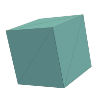
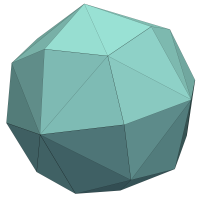
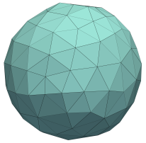
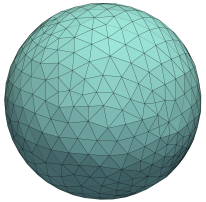
Figure 3. Tetrahedralizations of four different resolutions for the unit ball.

In order to measure the error to the approximate solution, we interpolate the exact solution to a mesh consisting of 12 047 801 finite elements (this is level $j=8$). This involves a mesh size of $h_{8}=0.0047$. For the levels $j=0,\ldots,7$, the mesh sizes and corresponding degrees of freedom (DoF) are given in Table 1. Moreover, we chose $N_{0}=10$ for the Monte Carlo quadrature and for the quasi-Monte Carlo quadrature and set $N_{\ell}=10\cdot 4^{\ell}$ and $N_{\ell}=10\cdot 2^{\ell}$, respectively. For the MLMC, in order to approximate the root mean square error, we average five realizations of the related approximation error. For the Clenshaw-Curtis quadrature, the number of samples are chosen as if there would hold $r=1$ in Lemma 6.4.

$\ell$	0	1	2	3	4	5	6	7
$h_{\ell}$	1.2	0.6	0.3	0.15	0.075	0.0375	0.0188	0.0094
$\operatorname{dof}_{\ell}$	8	27	244	1585	6042	29069	133376	551327

Table 1. Mesh sizes and DoF on the different levels for the unit ball.

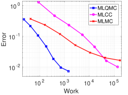
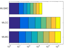
Figure 4. $H^{1}$-errors of the different quadrature methods (left) and number of samples on each level in case of $j=7$ (right) for the unit ball.

On the left side of Fig. 4, the error for the MLQMC, the MLCC and the MLMC is visualized. It is plotted against the work, which is expressed in terms of fine grid samples: In accordance with the degrees of freedom denoted in Table 1, we scale each sample on a particular level $\ell$ with the factor $\operatorname{DoF}_{\ell}/\operatorname{DoF}_{j}$, i.e. we weight a fine grid sample by $1$ and scale the coarse grid samples accordingly. The work is then given by summing up the total number of samples per level times the related weight.

It can be seen that MLQMC achieves the best error versus work rate. Moreover, the plot indicates that MLCC may asymptotically achieve a similar rate. MLMC seems to provide here only a halved rate compared to MLQMC. To give an insight on the number of samples spent on each particular level, we have depicted the corresponding numbers for $j=7$ on the right hand side of Fig. 4. It turns out that the quasi-Monte Carlo quadrature requires the smallest number of quadrature points. In contrast, the number of points for the Monte Carlo quadrature and for the Clenshaw-Curtis quadrature are nearly the same. This may be caused by the conservative choice for the number of quadrature points for the latter. Nevertheless, for fixed parameter dimension $m$ and $r=1$, we expect asymptotically similar rates for MLCC and MLQMC.

8.2. A more complex example

In our second example, the spatial domain is given by a model of the Zarya module of the International Space Station (ISS), which was the first module to be launched. Fig. 5 shows different tetrahedralizations of this geometry with decreasing mesh size. Note that the geometry can be imbedded into a cylinder with radius $0.52$ and height $1.58$.

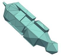
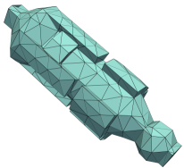
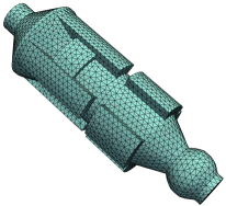
Figure 5. Tetrahedralizations of four different resolutions for the Zarya geometry.

Figure 6. Mean (left) and variance (right) of the model problem on the Zarya geometry.

$j$	0	1	2	3	4	5	6
$h_{j}$	0.5	0.25	0.125	0.0625	0.0313	0.0156	0.0078
$\operatorname{dof}_{j}$	174	333	1240	5846	30171	141029	617111

Table 2. Mesh sizes and DoF on the different levels for the Zarya geometry.

In this example, the parametric diffusion coefficient is given by

$${{a}}({{\bm{x}}},{{\bm{y}}})=1 +\frac{\exp({\|{{\bm{x}}}\|_{2}^{2}})}{20}\bigg{(}\sin(2\pi x_{1})y_{1}+\frac{1}{2}\sin(2\pi x_{2})y_{2}+\frac{1}{4}\sin(2\pi x_{3})y_{3}$$

$$+\frac{1}{8}\sin(4\pi x_{1})\sin(4\pi x_{2})y_{4}+\frac{1}{16}\sin(4\pi x_{1})\sin(4\pi x_{3})y_{5}$$

$$+\frac{1}{32}\sin(4\pi x_{2})\sin(4\pi x_{3})y_{6}\bigg{)}$$

and $f=10$. For ${{\bm{x}}}\in D$ and ${{\bm{y}}}\in{{\Gamma}}$, the diffusion coefficient varies approximately in the range $[0.19,1.81]$. Fig. 6 shows the mean (left) and the variance (right) of the reference solution. It has been computed on a mesh with 13 069 396 tetrahedrons resulting in a mesh size of $h=0.0039$ by 10 000 quasi-Monte Carlo samples based on the Halton sequence. For the levels $j=0,\ldots,6$, the mesh sizes and corresponding DoF are given in Table 2.

Fig. 7 visualizes the errors of the approximate expectation and second moment for the different multilevel quadrature methods under consideration. The number of quadrature points for the presented methods are chosen as in the previous example. Again, MLQMC provides the best error versus work rate in the mean, as well as in the second moment. The rates of MLMC and MLCC are both lower here.

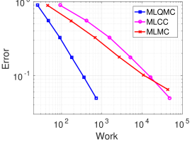
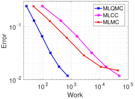
Figure 7. $H^{1}$-errors of the approximate mean (left) and $W^{1,1}$-errors of the approximate second moment (right) on the Zarya geometry for different quadrature methods.

9. Conclusion

In the present article, we have reversed the construction of the conventional multilevel quadrature. This enables us to give up the nestedness of the spatial approximation spaces. In particular, a polygonal approximation of curved domain boundaries is sufficient for computing the finite element solution. Hence, black-box finite element solvers can be directly applied to compute the solution of the underlying boundary value problem. Note that adaptively refined finite element meshes can be easily used as well. Another aspect of our approach is that the cost is considerably reduced by the application of nested quadrature formulae. Both features have been demonstrated by numerical results for the Clenshaw-Curtis quadrature and the quasi-Monte Carlo quadrature based on Halton points. Of course, other nested quadrature formulae like the Gauss-Patterson quadrature can be used as well. The application of quadrature formulae which are tailored to a possible anisotropy of the integrand is also straightforward. If non-nested quadrature formulae are applied, one arrives at a combination-technique-like representation of the multilevel quadrature.

References

• [1] I. Babuška, F. Nobile, and R. Tempone. A stochastic collocation method for elliptic partial differential equations with random input data. SIAM J. Numer. Anal., 45(3):1005–1034, 2007.
• [2] I. Babuška, R. Tempone, and G. Zouraris. Galerkin finite element approximations of stochastic elliptic partial differential equations. SIAM J. Numer. Anal., 42(2):800–825, 2004.
• [3] A. Barth, C. Schwab, and N. Zollinger. Multi-level Monte Carlo finite element method for elliptic PDEs with stochastic coefficients. Numer. Math., 119(1):123–161, 2011.
• [4] J. Beck, R. Tempone, F. Nobile, and L. Tamellini. On the optimal polynomial approximation of stochastic PDEs by Galerkin and collocation methods. Math. Models Methods Appl. Sci., 22(09):1250023, 2012.
• [5] D. Braess. Finite Elements. Theory, Fast Solvers, and Applications in Solid Mechanics. Cambridge University Press, Cambridge, 2nd edition, 2001.
• [6] S. Brenner and L. Scott. The Mathematical Theory of Finite Element Methods. Springer, Berlin, 3rd edition, 2008.
• [7] H.-J. Bungartz and M. Griebel. Sparse grids. Acta Numer., 13:147–269, 2004.
• [8] J. Charrier, R. Scheichl, and A. L. Teckentrup. Finite element error analysis of elliptic PDEs with random coefficients and its application to multilevel monte carlo methods. SIAM J. Numer. Anal., 51(1):322–352, 2013.
• [9] A. Cohen, R. DeVore, and C. Schwab. Convergence rates of best $N$-term Galerkin approximations for a class of elliptic sPDEs. Found. Comput. Math., 10:615–646, 2010.
• [10] A. Cohen, R. DeVore, and C. Schwab. Analytic regularity and polynomial approximation of parametric and stochastic elliptic PDEs. Anal. Appl., 09(01):11–47, 2011.
• [11] O. Ernst and B. Sprungk. Stochastic collocation for elliptic PDEs with random data: The lognormal case. In J. Garcke and D. Pflüger, editors, Sparse Grids and Applications — Munich 2012, pages 29–53. Springer International Publishing, Cham, 2014.
• [12] P. Frauenfelder, C. Schwab, and R. Todor. Finite elements for elliptic problems with stochastic coefficients. Comput. Methods Appl. Mech. Engrg., 194(2-5):205–228, 2005.
• [13] T. Gerstner and M. Griebel. Numerical integration using sparse grids. Numer. Algorithms, 18:209–232, 1998.
• [14] T. Gerstner and S. Heinz. Dimension- and time-adaptive multilevel Monte Carlo methods. In J. Garcke and M. Griebel, editors, Sparse Grids and Applications, volume 88 of Lecture Notes in Computational Science and Engineering, pages 107–120, Berlin-Heidelberg, 2012. Springer.
• [15] R. Ghanem and P. Spanos. Stochastic Finite Elements. A Spectral Approach. Springer, New York, 1991.
• [16] M. Giles. Multilevel Monte Carlo path simulation. Oper. Res., 56(3):607–617, 2008.
• [17] M. Giles. Multilevel Monte Carlo methods. Acta Numer., 24:259–328, 2015.
• [18] M. Giles and B. Waterhouse. Multilevel quasi-Monte Carlo path simulation. Radon Series Comp. Appl. Math., 8:1–18, 2009.
• [19] M. Griebel and H. Harbrecht. On the construction of sparse tensor product spaces. Math. Comput., 82(282):975–994, 2013.
• [20] A.-L. Haji-Ali, F. Nobile, E. von Schwerin, and R. Tempone. Optimization of mesh hierarchies in multilevel Monte Carlo samplers. Stoch. Partial Differ. Equ. Anal. Comput., 4(1):76–112, 2016.
• [21] J. Halton. On the efficiency of certain quasi-random sequences of points in evaluating multi-dimensional integrals. Numer. Math., 2(1):84–90, 1960.
• [22] H. Harbrecht, M. Peters, and M. Siebenmorgen. On multilevel quadrature for elliptic stochastic partial differential equations. In J. Garcke and M. Griebel, editors, Sparse Grids and Applications, volume 88 of Lecture Notes in Computational Science and Engineering, pages 161–179, Berlin-Heidelberg, 2012. Springer.
• [23] H. Harbrecht, M. Peters, and M. Siebenmorgen. Efficient approximation of random fields for numerical applications. Numer. Linear Algebra Appl., 22(4):596–617, 2015.
• [24] H. Harbrecht, M. Peters, and M. Siebenmorgen. Analysis of the domain mapping method for elliptic diffusion problems on random domains. Numer. Math., 134(4):823–856, 2016.
• [25] H. Harbrecht, M. Peters, and M. Siebenmorgen. Multilevel accelerated quadrature for PDEs with log-normally distributed diffusion coefficient. SIAM/ASA J. Uncertain. Quantif., 4(1):520–551, 2016.
• [26] H. Harbrecht, M. Peters, and M. Siebenmorgen. On the quasi-Monte Carlo method with Halton points for elliptic PDEs with log-normal diffusion. Math. Comp., 86:771–797, 2017.
• [27] S. Heinrich. The multilevel method of dependent tests. In Advances in stochastic simulation methods (St. Petersburg, 1998), Stat. Ind. Technol., pages 47–61. Birkhäuser, Boston, MA, 2000.
• [28] S. Heinrich. Multilevel Monte Carlo methods. In Lecture Notes in Large Scale Scientific Computing, pages 58–67, London, 2001. Springer.
• [29] E. Hille and R. Phillips. Functional Analysis and Semi-Groups, volume 31 of American Mathematical Society Colloquium Publications. American Mathematical Society, Providence, 1957.
• [30] V. Hoang and C. Schwab. $N$-term Wiener chaos approximation rate for elliptic PDEs with lognormal Gaussian random inputs. Math. Models Methods Appl. Sci., 4(24):797–826, 2014.
• [31] F. Kuo, C. Schwab, and I. Sloan. Multi-level quasi-Monte Carlo finite element methods for a class of elliptic partial differential equations with random coefficients. Found. Comput. Math., 15(2):411–449, 2015.
• [32] M. Loève. Probability theory. I+I​I, volume 45 of Graduate Texts in Mathematics. Springer, New York, 4th edition, 1977.
• [33] H. Matthies and A. Keese. Galerkin methods for linear and nonlinear elliptic stochastic partial differential equations. Comput. Methods Appl. Mech. Engrg., 194(12-16):1295–1331, 2005.
• [34] H. Niederreiter. Random Number Generation and Quasi-Monte Carlo Methods. Society for Industrial and Applied Mathematics, Philadelphia, PA, USA, 1992.
• [35] E. Novak and K. Ritter. High dimensional integration of smooth functions over cubes. Numer. Math., 75(1):79–97, 1996.
• [36] C. Schwab and R. Todor. Karhunen-Loève approximation of random fields by generalized fast multipole methods. J. Comput. Phys., 217:100–122, 2006.
• [37] M. Siebenmorgen. Quadrature methods for elliptic PDEs with random diffusion. PhD Thesis, Faculty of Science, University of Basel, 2015.
• [38] A. Teckentrup, R. Scheichl, M. Giles, and E. Ullmann. Further analysis of multilevel Monte Carlo methods for elliptic PDEs with random coefficients. Numer. Math., 125(3):569–600, 2013.
• [39] A. L. Teckentrup, P. Jantsch, C. G. Webster, and M. Gunzburger. A multilevel stochastic collocation method for partial differential equations with random input data. SIAM/ASA J. Uncertain. Quantif., 3(1):1046–1074, 2015.
• [40] R. Todor and C. Schwab. Convergence rates for sparse chaos approximations of elliptic problems with stochastic coefficients. IMA J. Numer. Anal., 27(2):232–261, 2007.
• [41] X. Wang. A constructive approach to strong tractability using quasi-Monte Carlo algorithms. J. Complexity, 18:683–701, 2002.