Historical Graph Data Management

Storing and Analyzing Historical Graph Data at Scale

Abstract

The work on large-scale graph analytics to date has largely focused on the study of static properties of graph snapshots. However, a static view of interactions between entities is often an oversimplification of several complex phenomena like the spread of epidemics, information diffusion, formation of online communities, and so on. Being able to find temporal interaction patterns, visualize the evolution of graph properties, or even simply compare them across time, adds significant value in reasoning over graphs. However, because of lack of underlying data management support, an analyst today has to manually navigate the added temporal complexity of dealing with large evolving graphs. In this paper, we present a system, called Historical Graph Store, that enables users to store large volumes of historical graph data and to express and run complex temporal graph analytical tasks against that data. It consists of two key components: a Temporal Graph Index (TGI), that compactly stores large volumes of historical graph evolution data in a partitioned and distributed fashion; it provides support for retrieving snapshots of the graph as of any timepoint in the past or evolution histories of individual nodes or neighborhoods; and a Spark-based Temporal Graph Analysis Framework (TAF), for expressing complex temporal analytical tasks and for executing them in an efficient and scalable manner. Our experiments demonstrate our system’s efficient storage, retrieval and analytics across a wide variety of queries on large volumes of historical graph data.

1 Introduction

Graphs are useful in capturing behavior involving interactions between entities. Several processes are naturally represented as graphs – social interactions between people, financial transactions, biological interactions among proteins, geospatial proximity of infected livestock, and so on. Many problems based on such graph models can be solved using well-studied algorithms from graph theory or network science. Examples include finding driving routes by computing shortest paths on a network of roads, finding user communities through dense subgraph identification in a social network, and many others. Numerous graph data management systems have been developed over the last decade, including specialized graph database systems like Neo4j, Titan, etc., and large-scale graph processing frameworks such as Pregel [36], Giraph, GraphLab [34], GraphX [20], GraphChi [31], etc.

However much of the work to date, especially on cloud-scale graph data management systems, focuses on managing and analyzing a single (typically, current) static snapshot of the data. In the real world, however, interactions are a dynamic affair and any graph that abstracts a real-world process changes over time. For instance, in online social media, the friendship network on Facebook or the “follows” network on Twitter change steadily over time, whereas the “mentions” or the “retweet” networks change much more rapidly. Dynamic cellular networks in biology, evolving citation networks in publications, dynamic financial transactional networks, are few other examples of such data. Lately, we have seen an increasing merit in dynamic modeling and analysis of network data to obtain crucial insights in several domains such as cancer prediction [49], epidemiology [23], organizational sociology [24], molecular biology [14], information spread on social networks [33] amongst others.

In this work, our focus is on providing the ability to analyze and to reason over the entire history of the changes to a graph. There are many different types of analyses of interest. For example, an analyst may wish to study the evolution of well-studied static graph properties such as centrality measures, density, conductance, etc., over time. Another approach is through the search and discovery of temporal patterns, where the events that constitute the pattern are spread out over time. Comparative analysis, such as juxtaposition of a statistic over time, or perhaps, computing aggregates such as max or mean over time, possibly gives another style of knowledge discovery into temporal graphs. Most of all, a primitive notion of just being able to access past states of the graphs and performing simple static graph analysis, empowers a data scientist with the capacity to perform analysis in arbitrary and unconventional patterns.

Supporting such a diverse set of temporal analytics and querying over large volumes of historical graph data requires addressing several data management challenges. Specifically, there is a want of techniques for storing the historical information in a compact manner, while allowing a user to retrieve graph snapshots as of any time point in the past or the evolution history of a specific node or a specific neighborhood. Further the data must be stored and queried in a distributed fashion to handle the increasing scale of the data. We must also develop an expressive, high-level, easy-to-use programming framework that will allow users to specify complex temporal graph analysis tasks, while ensuring that the specified tasks can be executed efficiently in a data-parallel fashion across a cluster.

In this paper, we present a graph data management system, called Historical Graph Store (HGS), that provides an ecosystem for managing and analyzing large historical traces of graphs. HGS consists of two key distinct components. First, the Temporal Graph Index (TGI), is an index that compactly stores the entire history of a graph by appropriately partitioning and encoding the differences over time (called deltas). These deltas are organized to optimize the retrieval of several temporal graph primitives such as neighborhood versions, node histories, and graph snapshots. TGI is designed to use a distributed key-value store to store the partitioned deltas, and can thus leverage the scalability afforded by those systems (our implementation uses Apache Cassandra key-value store). TGI is a tunable index structure, and we investigate the impact of tuning the different parameters through an extensive empirical evaluation. TGI builds upon our prior work on DeltaGraph [29], where the focus was on retrieving individual snapshots efficiently; we discuss the differences between the two in more detail in Section 4.

The second component of HGS is a Temporal Graph Analysis Framework (TAF), which provides an expressive library to specify a wide range of temporal graph analysis tasks and to execute them at scale in a cluster environment. The library is based on a novel set of temporal graph operators that enable a user to analyze the history of a graph in a variety of manners. The execution engine itself is based on Apache Spark [54], a large-scale in-memory cluster computing framework.

Outline: The rest of the paper is organized as follows. In Section 2, we survey the related work on graph data stores, temporal indexing, and other topics relevant to the scope of the paper. In Section 3, we provide a sketch of the overall system, including key aspects of the underlying components. We then present the Temporal Graph Index and the Temporal Graph Analytics Framework in detail in Section 4 and Section 5, respectively. In Section 6, we provide an empirical evaluation of the various system components such as the graph retrieval, scalability of temporal analytics, etc. We conclude with a summary and a list of future directions in Section 7.

2 Related Work

In the recent years, there has been much work on graph storage and graph processing systems and numerous systems have been designed to address various aspects of graph data management. Some examples include Neo4J, AllegroGraph [1], Titan, GBase [28], Pregel [36], Giraph, GraphChi [31], GraphX [20], GraphLab [34], and Trinity [43]. These systems use a variety of different models for representation, storage, and querying, and there is a lack of standardized or widely accepted models for the same. Most graph querying happens through programmatic access to graphs in languages such as Java, Python or C++. Graph libraries such as Blueprints provide a rich set of implementations for graph theoretic algorithms. SPARQL [40] is a language used to search patterns in linked data. It works on an underlying RDF representation of graphs. T-SPARQL [21] is a temporal extension of SPARQL. He et al. [26], provide a language for finding sub-graph patterns using a graph as a query primitive. Gremlin is a graph traversal language over the property graph data model, and has been adopted by several open-source systems. For large-scale graph analysis, perhaps the most popular framework is the vertex-centric programming framework, adopted by Giraph, GraphLab, GraphX, and several other systems; there have also been several proposals for richer and more expressive programming frameworks in recent years. However, most of these prior systems largely focus on analyzing a single snapshot of the graph data, with very little support for handling dynamic graphs, if any.

A few recent papers address the issues of storage and retrieval in dynamic graphs. In our prior work, we proposed DeltaGraph [29], an index data structure that compactly stores the history of all changes in a dynamic graph and provides efficient snapshot reconstruction. G* [32] stores multiple snapshots compactly by utilizing commonalities. Chronos [25, 37] is an in-memory system for processing dynamic graphs, with objective of shared storage and computation for overlapping snapshots. Ghrab et al. [19] provide a system of network analytics through labeling graph components. Gedik et al. [17], describe a block-oriented and cache-enabled system to exploit spatio-temporal locality for solving temporal neighborhood queries. Koloniari et al. also utilize caching to fetch selective portions of temporal graphs they refer to as partial views [30]. LLAMA [35] uses multiversioned arrays to represent a mutating graph, but their focus is primarily on in-memory representation. There is also recent work on streaming analytics over dynamic graph data [11, 10], but it typically focuses on analyzing only the recent activity in the network (typically over a sliding window). Our work in this paper focuses on techniques for a wide variety of temporal graph retrieval and analysis on entire graph histories.

Temporal graph analytics is an area of growing interest. Evolution of shortest paths in dynamic graphs has been studies by Huo et al. [27], Ren et al. [41], and Xuan et al. [53]. Evolution of community structures in graphs has been of interest as well [4, 7, 22, 47]. Change in page rank with evolving graphs [13, 5], and the study of change in centrality of vertices, path lengths of vertex pairs, etc. [39], also lie under the larger umbrella of temporal graph analysis. Ahn et al. [2] provide a taxonomy of analytical tasks over evolving graphs. Barrat et al. [6], provide a good reference for studying several dynamic processes modeled over graphs. Our system significantly reduces the effort involved in building and deploying such analytics over large volumes of graph data.

Temporal data management for relational databases was a topic of active research in the 80s and early 90s. Snapshot index [50] is an I/O optimal solution to the problem of snapshot retrieval for transaction-time databases. Salzberg and Tsotras [42] present a comprehensive survey of temporal data indexing techinques, and discuss two extreme approaches to supporting snapshot retrieval queries, referred to as the Copy and Log approaches. While the copy approach relies on storing new copies of a snapshot upon every point of change in the database, the log approach relies on storing everything through changes. Their hybrid is often referred to as the Copy+Log approach. We omit a detailed discussion of the work on temporal databases, and refer the interested reader to a representative set of references [9, 45, 38, 48, 12, 44, 42]. Other data structures, such as Interval Trees [3] and Segment trees [8] can also be used for storing temporal information. Temporal aggregation in scientific array databases [46] is another related topic of interest, but the challenges there are significantly different.

3 Overview

In this section, we introduce key aspects related to HGS. We begin with the data model, followed by the key challenges and concluding with an overview of the system.

3.1 Data Model

Under a discreet notion of time, a time-evolving graph $G^{T}=(V^{T},E^{T})$ may be expressed as a collection of graph snapshots over different time points, $\{G^{0}=(V^{0},E^{0}),G^{1},\dots,G^{t}\}$. The vertex set $V^{i}$ for a snapshot consists of a set of vertices (nodes), each of which has a unique identifier, and an arbitrary number of key-value attribute pairs. The edge sets $E^{i}$ consist of edges that each contain references to two valid nodes in the corresponding vertex set $V^{i}$, information about the direction of the edge, and an arbitrary list of key-value attribute pairs. A temporal graph can also be equivalently described by a set of changes to the graph over time. We call an atomic change at a specific timepoint in the graph an event. The changes could be structural, such as the addition or the deletion of nodes or edges, or be related to attributes such as an addition or a deletion or a change in the value of a node or an edge attribute. These approaches as well as certain hybrids have been used in the past for the physical and logical modeling of temporal data. Our approach to temporal processing in this paper is best described using a node-centric logical model, i.e., the historical graph is seen as a collection of evolving vertices over time; the edges are considered as attributes of the nodes.

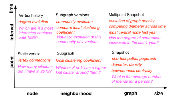
Figure 1: The scope of temporal graph analytics can be represented across two different dimensions - time and entity. The chart lists retrieval tasks (black), graph operations (red), example queries (magenta) at different granularities of time and entity size.

3.2 Challenges

The nature of data management tasks in historical graph analytics can be categorized based on the scope of analysis using the dual dimensions of time and entity as illustrated with examples in Figure 1. The temporal scope of an analysis task can range from a single point in time to a long interval; the entity scope can range from a single node to the entire graph. While the diversity of analytical tasks provides a potential for a rich set of insights from historical graphs, it also poses several challenges in constructing a system that can perform those tasks. To the best of our knowledge, none of the existing systems address a majority of those challenges that are described below:

Compact storage with fast access: An natural tradeoff between index size and access latencies can be seen in the Log and Copy approaches for snapshot retrieval. Log requires minimal information for encoding the graph’s history, but incurs large reconstruction costs. Copy, on the other hand, provides direct access, but at the cost of excessive storage. The desirable index should consume space of the order of Log index but provide near direct access like Copy.

Time-centric versus entity-centric indexing: For point access such as past snapshot retrieval, a time-centric indexing such as DeltaGraph or Copy+Log is suitable. However, for version retrieval tasks such as retrieving a node’s history, entity-centric indexing is the correct choice. Neither of the indexing approaches, however, are feasible in the opposite scenarios. Given the diversity of access needs, we require an index that works well with both styles of lookup at the same time.

Optimal granularity of storage for different queries: Query latencies for a graph also depends on the size of chunks in which the data is indexed. While larger granularities of storage incur wasteful data read for “node retrieval”, a finely chunked graph storage would mean higher number of lookups and aggregation for a 2-hop neighborhood lookup. The physical and logical arrangement of data should take care of access needs of queries of all granularities.

Coping with changing topology in a dynamic graph: It is evident that graph partitioning is inevitable in the storage and processing of large graphs. However, finding the appropriate strategy to maintain workable partitioning on a constantly changing graph is another challenge while designing a historical graph index.

Systematically expressing temporal graph analytics: A platform for expressing a wide variety of historical graph analytics requires an appropriate amalgam of temporal logic and graph theory. Additionally, utilizing a vast body of existing tools in network science is an engineering challenge and opportunity.

Appropriate abstractions for distributed, scalable analytics: Parallelization is the key to scale up analytics for large network datasets. It is essential that the underlying data-representations and operators in the analytical platform be designed for parallel computing.

3.3 System Overview

Figure 2 shows the architecture of our proposed Historical Graph Store. It consists of two main components:

Temporal Graph Index (TGI) records the entire history of a graph compactly while enabling efficient retrieval of several temporal graph primitives. It encodes various forms of differences (called deltas) in the graph, such as atomic events, changes in subgraphs over intervals of time, etc. It uses specific choices of graph partitioning, data replication, temporal compression and data placement to optimize the graph retrieval performance. TGI uses the Apache Cassandra distributed key-value store as the backend to store the deltas. In Section 4, we describe the design details of TGI and the access algorithms.

Temporal Graph Analytics Framework (TAF) provides a temporal node-centric abstraction for specifying and executing complex temporal network analysis tasks. We provide a Java and Python based library to specify the retrieval, computation and analysis on a set of (temporal) nodes (SoN). Computational scalability is achieved by distributing tasks by node and time. TAF is built on top of Apache Spark for supporting scalable, in-memory, cluster computation and provides an option to utilize GraphX for static graph computation. In Section 5, we describe the details of the library, query processing, parallel data fetch aspects of the system, along with a few examples of analytics.

Figure 2: System Overview

4 Temporal Graph Index

In this section, we investigate the issue of indexing temporal graphs. First, we introduce a delta framework to define any temporal index as a set of different changes or deltas. Using this framework, we are able to qualitatively compare the access costs and sizes of different alternatives for temporal graph indexing, including our proposed approach. We then present the Temporal Graph Index (TGI), that stores the entire history of a large evolving network in the cloud, and facilitates efficient parallel reconstruction for different graph primitives. TGI is a generalization of both entity and time-based indexing approaches and can be tuned to suit specific workload needs. We claim that TGI is the minimal index that provides efficient access to a variety of primitives on a historical graph, ranging from past snapshots to versions of a node or neighborhood. We also describe the key partitioning strategies instrumental in scaling to large datasets across a cloud storage.

4.1 Preliminaries

We start with a few preliminary definitions that help us formalize the notion of the delta framework.

Definition 1 (Static node)

A static node refers to the state of a vertex in a network at a specific time, and is defined as a set containing: (a) node-id, denoted I (an integer), (b) an edge-list, denoted E (captured as a set of node-ids), (c) attributes, denoted A, a map of key-value pairs.

A static edge is defined analogously, and contains the node-ids for the two endpoints and the edge direction in addition to a map of key-value pairs. Finally, a static graph component refers to either a static edge or a static node.

Definition 2 (Delta)

A Delta ($\Delta$) refers to either: (a) a static graph component (including the empty set), or (b) a difference, sum, union or intersection of two deltas.

Definition 3 (Cardinality and Size)

The cardinality
and the size of a $\Delta$ are the unique and total number of static node or edge descriptions within it, respectively.

Definition 4 ($\Delta$ Sum)

A sum (+) over two deltas, $\Delta_{1}$ and $\Delta_{2}$, i.e., $\Delta_{s}=\Delta_{1}+\Delta_{2}$ is defined over graph components in the two deltas as follows: (1) $\forall gc_{1}\in\Delta_{1}$, if $\exists gc_{2}\in\Delta_{2}\ s.t.\ gc_{1}.I=gc_{2}.I$, then we add $gc_{2}$ to $\Delta_{s}$, (2) $\forall gc_{1}\in\Delta_{1}\ s.t.\ \nexists gc_{2}\in\Delta_{2}\ s.t.\ gc_{1}.I=gc_{2}.I$, we add $gc_{1}$ to $\Delta_{s}$, and (3) analogously the components present only in $\Delta_{2}$ are added to $\Delta_{s}$.

Note that: $\Delta_{1}+\Delta_{2}=\Delta_{2}+\Delta_{1}$ is not necessarily true due the order of changes. We also note that: $\Delta_{1}+\emptyset=\Delta_{1}$, and $(\Delta_{1}+\Delta_{2})+\Delta_{3}=\Delta_{1}+(\Delta_{2}+\Delta_{3})$. Analogously, difference(-) is defined as a set difference over different components of the two deltas. $\Delta_{1}-\phi=\Delta_{1}$ and $\Delta_{1}-\Delta_{1}=\phi$, are true, while, $\Delta_{1}-\Delta_{2}=\Delta_{2}-\Delta_{1}$, does not necessarily hold.

Definition 5 ($\Delta$ Intersection)

An intersection of two $\Delta$s is defined as a set intersection over the the components of two deltas. $\Delta_{1}\cap\phi=\phi$, is true for any delta. Similarly, union of two deltas $\Delta_{\cup}=\Delta_{1}\cup\Delta_{2}$, consists of all elements from $\Delta_{1}$ and $\Delta_{2}$. The following is true for any delta: $\Delta_{1}\cup\phi=\Delta_{1}$.

Next we discuss and define some specific types of $\Delta$s:

Example 1 (Event)

An event is the smallest change that happens to a graph, i.e., addition or deletion of a node or an edge, or a change in an attribute value. An event is described around one time point. As a $\Delta$, an event concerning a graph component $c$, at time point $t_{e}$, is defined as the difference of state of $c$ at and before $t_{e}$, i.e., $\Delta_{event}(c,t_{e})=c(t_{e})-c(t_{e}-1)$.

Example 2 (Eventlist)

An eventlist delta is a chronologically sorted set of event deltas. An eventlist’s scope may be defined by the time duration, $(t_{s},t_{e}]$, during which it defines all the changes that happened to the graph.

Example 3 (Partitioned Eventlist)

An partitioned eventlist delta is an eventlist constrained by the scope of a set of nodes (say a set of nodes, $\mathcal{N}=\{N_{1},N_{2},\dots\})$ apart from the time range constraint $(t_{s},t_{e}]$.

Example 4 (Snapshot)

A snapshot, $\mathcal{G}^{t_{a}}$ is the state of a graph $\mathcal{G}$ at a time point $t_{a}$. As a $\Delta$, it is defined as the difference of the state of the graph at $t_{a}$ from an empty set, $\Delta_{snapshot}({\mathcal{G}},t_{a})=G(t_{a})-G(-\infty)$.

Example 5 (Partitioned Snapshot)

A partitioned snapshot is a subset of a snapshot. It is identified by a subset of all nodes, $\mathcal{P}$ in graph, $\mathcal{G}$ at time, $t_{a}$. It consists of the state of all nodes at time $t_{a}$ and all the edges whose at least one of the end points lies in $\mathcal{P}$ at time, $t_{a}$.

4.2 Prior Techniques

The prior techniques for temporal graph indexing use changes or differences in various forms to encode time-evolving datasets. We can express them in the $\Delta$ framework as follows. The Log index is equivalent to a set of all event deltas (equivalently, a single eventlist delta encompassing the entire history). The Copy+Log index can be represented as combination of: (a) a finite number of distinct snapshot deltas, and (b) eventlist deltas to capture the change between successive snapshots. Although we are not aware of a specific proposal for a vertex-centric index, however, a natural approach would be to maintain a set of partitioned eventlist deltas, one for each node (with edge information replicated with the endpoints). The DeltaGraph index, proposed in our prior work, is a tunable index with several parameters. For a typical setting of parameters, it can be seen as equivalent to taking a Copy+Log index, and replacing the snapshot deltas in it with another set of deltas constructed hierarchically as follows: for every $k$ successive snapshot deltas, replace them with a single delta that is the intersection of those deltas and a set of difference deltas from the intersection to the original snapshots, and recursively apply this till you are left with a single delta.

Table 1 estimates the cost of fetching different graph primitives as the number and the cumulative size of deltas that need to be fetched for the different indexes. The first column shows an estimate of the total storage space, which varies considerably across the techniques.

	Index	Snapshot		Static Vertex		Vertex versions		1-hop		1-hop Versions
	Size	$\sum_{\Delta}{|\Delta|}$	$\sum_{\Delta}{1}$	$\sum_{\Delta}{|\Delta|}$	$\sum_{\Delta}{1}$	$\sum_{\Delta}{|\Delta|}$	$\sum_{\Delta}{1}$	$\sum_{\Delta}{|\Delta|}$	$\sum_{\Delta}{1}$	$\sum_{\Delta}{|\Delta|}$	$\sum_{\Delta}{1}$
Log	$|G|$	$|G|$	$|G|\over|E|$	$|G|$	$|G|\over|E|$	$|G|$	$|G|\over|E|$	$|G|$	$|G|\over|E|$	$|G|$	$|G|\over|E|$
Copy	$|G|^{2}$	$|S|$	$1$	$|S|$	$1$	$|S||G|$	$|G|$	$|S|$	$1$	$|S||G|$	$|G|$
Copy+Log	${|G|^{2}\over|E|}$	$|S|+|E|$	$2$	$|S|+|E|$	2	$|G|$	$|G|\over|E|$	$|S|+|E|$	2	$|G|$	$|G|\over|E|$
Node Centric	$2|G|$	$2.|G|$	$|N|$	$|C|$	$1$	$|C|$	1	$|R|.|V|$	$|R|$	$|R|.|V|$	$|R|$
DeltaGraph	$X_{1}^{*}$	h.$|S|+|E|$	$2h$	$h.|S|+|E|$	$2h$	$|G|$	$|G|\over|E|$	$h.(|S|+|E|)$	2h	$|G|$	$|G|\over|E|$
TGI	$X_{2}^{**}$	h.$|S|+|E|$	$2h$	${h.|S|\over p}+{|E|\over p}$	$2h$	$|V|(1+{|S|\over p})$	$|V|+1$	${h.(|S|+|E|)\over p}$	2h	$|V|(1+{|S|\over p})$	$|V|+1$

Table 1: Comparison of access costs for different retrieval queries and index storage on various temporal indexes. $|G|=$number of changes in the graph; $|S|=$size of a snapshot; $h=$ height and $|E|=$ eventlist size in C+L, DG or TGI; $|V|=$number of changes to a node; $|R|$=numbers of neighbors of a node; $p$= number of partitions in TGI. The metrics used are the sum of delta cardinalities ($\sum_{\Delta}{|\Delta|}$) and the number of deltas ($\sum_{\Delta}{1}$). For reasons of space, ${}^{*}X_{1}=|G|(h+1)$; ${}^{**}X_{2}=|G|(2h+3)$.

4.3 Temporal Graph Index: Definition

Given the above formalism, a Temporal Graph Index for a graph $\mathcal{G}$ over a time period $T=[0,t_{c}]$ is described by a collection of different $\Delta$s as follows:

• Partitioned Eventlists: A set of partitioned eventlist $\Delta$s, $\{E_{tp}\}$, where $E_{tp}$ captures the changes during the time interval $t$ belonging to partition $p$.

• Derived Partitioned Snapshots: Consider $r$ distinct time points, $t_{i}$, where $1\leq i\leq r$, $t_{i}\in T$, For each $t_{i}$, we consider $l$ partition $\Delta$s, $P_{j}^{i}$, $1<j<l$, such that $\cup_{j}P_{j}^{i}={\mathcal{G}^{t_{i}}}$. There exists a function that maps any node-id(I) in $\mathcal{G}^{t_{i}}$ to a unique partition-id($P_{j}^{i}$), $f_{i}:I\rightarrow P_{j}^{i}$. With a collection of $P_{j}^{i}$ over $T$ as leaf nodes, we construct a hierarchical tree structure where a parent is the intersection of children deltas. The difference of each parent from its child delta is called as a derived partitioned snapshot and is explicitly stored. Note that $P_{j}^{i}$’s are not explicitly stored. This is the same as DeltaGraph, with the exception of partitioning.

• Version Chain: For all nodes $\mathcal{N}$ in the graph $\mathcal{G}$, we maintain a chronologically sorted list of pointers to all the references for that node in the delta sets described above (a and b). For a node $I$, this is called a version chain($VC_{I}$).

In short, the TGI stores deltas or changes in three different forms, as follows. The first one is the atomic changes in a chronological order through partitioned eventlists. This facilitates direct access to the changes that happened to a part or whole of the graph at specified points in time. Secondly, the state of nodes at different points in time is stored indirectly in form of the derived partitioned snapshot deltas. This facilitates direct access to the state of a neighborhood or the entire graph at a given time. Thirdly, a meta index stores node-wise pointers to the list of chronological changes for each node. This gives us a direct access to the changes occurring to individual nodes. Figure 3(a) shows the arrangement of eventlist, snapshot and derived snapshot partitioned deltas. Figure 3(b) shows a sample version chain.

TGI utilizes the concept of temporal consistency which was optimally utilized by DeltaGraph. However, it differs from DeltaGraph in two major ways. First, it uses a partitioning for eventlists, snapshots or deltas instead of a large monolithic chunks. Additionally, it maintains a list of version chain pointers for each node. The combination of these two novelties along with DeltaGraph’s temporal compression generalizes the notion of entity-centric and time-centric indexing approaches in an efficient way. This can be seen by the qualitative comparison shown in Table 1 as well as empirical results in Section 6.

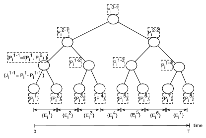
(a) TGI deltas - partitioned eventlists, snapshots and derived snapshots. The (dotted) bounded deltas are not stored.

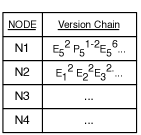
(b) Version Chains

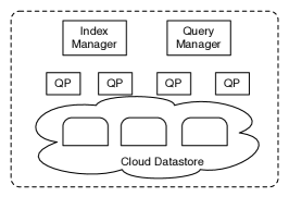
(c) Architecture

Figure 3: Temporal Graph Index representation.

4.4 TGI: Design and Architecture

In the previous subsection, we presented the logical description of TGI. We now describe the strategies for physical storage on a cloud which enables high scalability. In a distributed index, we desire that all graph retrieval calls achieve maximum parallelization through equitable distribution. A distribution strategy based on pure node-based key is good idea for snapshot style access, however, it is bad for a subgraph history style of access. A pure time-based key strategy on the other hand, has complementary qualities and drawbacks. An important related challenge for scalability is dealing with two different skews in a temporal graph dataset – temporal and topological. They refer to the uneven density of graph activity over time and the uneven edge density across regions of the graph, respectively. Another important aspect to note is that for a retrieval task, it is desirable that all the required micro-deltas on a particular machine be proximally located to minimize latency of lookups.

Based on the above constraints and desired properties, we describe the physical layout of TGI as follows:

1. The entire history of the graph is divided into time spans, keeping the number of changes to the graph consistent across different time spans, $f_{t}:e.time\rightarrow tsid$, where $e$ is the event and $tsid$ is the unique identifier for the time span. This is illustrated in Figure 4.

2. A graph at any point is horizontally partitioned into a fixed number of horizontal partitions based upon a random function of the node-id, $f_{h}:nid\rightarrow sid$, where $nid$ is the node-id and $sid$ is unique identifier of for the horizontal partition.

3. The micro-deltas (including eventlists) are stored as a key-value pairs, where the delta-key is composed of
   $\{tsid,sid,did,pid\}$, where $did$ is a delta-id, and $pid$ is the partition-id of the micro-delta.

4. The placement-key is defined as a subset of the composite deltas key described above, as $\{tsid,sid\}$, which defines the chunks in which data is placed across a set of machines on a cluster. A combination of the $tsid$ and $sid$ ensure that a large fetch task, whether snapshot or version oriented, seeks data distributed across the cluster and not just one machine.

5. The micro-deltas are clustered by the delta key. The given order of the delta-key besides the placement-key elements, means that all the micro-partitions of a delta are stored contiguously, which makes it efficient to scan and read all micro-partitions belonging to a delta in a snapshot query. On the other hand, if the order of $did$ and $pid$ is reversed, it makes fetching a micro-partition across different deltas more efficient.

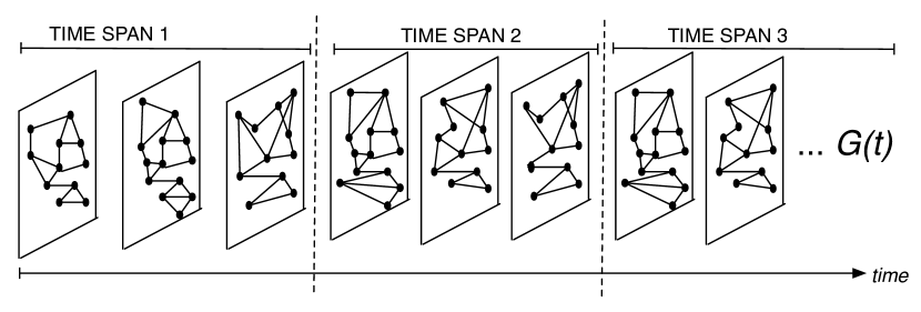
Figure 4: The graph history is divided into non-overlapping periods of time. Such division is based on time intervals after which the locality-based graph partitioning is updated. It is also used as a partial key for data chunking and placement.

Irrespective of a temporal or a topological skew in the graph, the index is spread out across a cluster in a balanced manner. This also makes it possible to fetch the graph primitives of large sizes in a naturally parallel manner. For instance, a snapshot query would demand all micro-partitions for a specific set of deltas in a particular timespan across all horizontal partitions. Given an equitable distribution of the deltas across all machines of a cluster, we retrieve the data in parallel on each storage machine, without a considerable skew.

Implementation: TGI uses Cassandra for its delta storage. There are 5 tables that contain TGI data and metadata:
(1) Deltas(tsid, sid, did, pid, dval) table stores the deltas as described above, where dval contains serialized value of the micro-delta as a binary string.
(2) Versions(nid, vchain) consists of each node’s version chain as a hash-table with keys for each timespan.
(3) Timespans(tsid, start, end, checkpts, k, df) stores, for each timespan, start and end times, a list of snapshot checkpoints, and arity.
(4) Graph(start, end, events, tscount, gtype) contains global information about the graph and TGI.
(5) Micropartitions(nid, tsid, pid) contains micro-delta partitioning information about nodes. It is not utilized in case of random partitioning.
The graph construction and fetching modules are written in Python, using Pickle and Twisted libraries for serialization and communication.

Architecture: TGI architecture can be seen in Figure 3c, where Query Mananger (QM) is responsible for planning, dividing and delegating the query to one or more Query Processors (QP). The QPs query the datastore in parallel and process the raw deltas into the required result. Depending on the query specification, the distributed result is either aggregated at a particular QP (the QM) or returned to the client which made the request without aggregation. The Index Manager is responsible for the construction and maintenance activities of the index. The cloud represents the distributed datastore.

Construction and Update: The construction process involves three different stages. First, we analyze the input data using the index construction parameters including the timespan length (ts), number of horizontal partitions (ns), number of likely datastore nodes (m), eventlist size (l), and micro-delta partition size (psize). In the second stage, the input data is split into horizontal partitions. In the third stage, parallel construction workers of the IM work on separate horizontal partitions, and build the index, a time span at a time. The process of construction of each timespan is similar to that of DeltaGraph, albeit more fine-grained due to delta partitioning and version chain construction as well. The TGI accepts updates of events in batches of timespan length. The update process involves creating an independent TGI with the new events, and merging it with the original TGI. The merger of TGIs involves updates of corresponding deltas, VC index and the metadata.

4.5 Dynamic Graph Partitioning

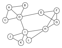
(a) Graph Snapshot.

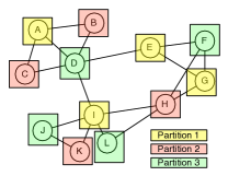
(b) Random partitioning of graph snapshot with high number of edge-cuts.

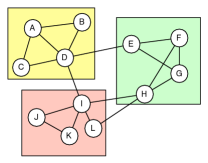
(c) Min-cut partitioning of snapshot.

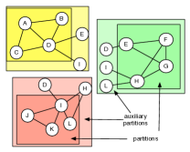
(d) Min-cut partitioning of snapshot with edge-cut replication and auxiliary storage strategy.

Figure 5: Graph partitioning using min-cut strategy along with 1-hop replication and the use of auxiliary micro-deltas improves 1-hop neighborhood retrieval performance without affecting the performance of snapshot or node retrieval.

Partitioning deltas into micro-deltas is an essential aspect of TGI and provides cheaper access to subgraph elements when compared to DeltaGraph or similar indexes. In a time-evolving graph, however, the size and topology of the graph change with time. The key is to keep the size of each micro-delta (and each micro-eventlist) about the same and bounded by a number that dictates the latency for fetching a node or neighborhood. The two traditional approaches to partitioning a static graph are random (node-id hash-based) or locality-based (min-cut max-flow) partitioning. Random partitioning is simpler and involves minimal bookkeeping. However, since it loses locality, it is unsuitable for neighborhood-level granularity access. Locality-aware partitioning, on the other hand, preserves locality but incurs extra bookkeeping in form of a {node-id:partition-id} map. TGI is designed to work with either configuration as desired, as well as different partition size specifications. TGI also supports replication of edge-cuts for further speed up of 1-hop neighborhoods. It uses a separate auxiliary micro-delta besides each micro-delta to store the replication, thereby preventing extra read cost for snapshot or node centric queries. This is illustrated in Figure 5.

Locality-aware partitioning, however, faces an additional challenge with time-evolving graphs. With the change in size and topology of a graph, a partitioning deemed good (with respect to locality) at an instant may cease to be good at a later time. A probable approach of frequent repartitioning over time would maintain partitioning quality, but leads to excessive amounts of bookkeeping, which in turn leads to degradation of performance while accessing different node or neighborhood versions. Maintaining and looking up that map as frequently as the changes in the graph is highly inefficient. Hence, we divide the history of the graph into time spans, where we keep the partitioning consistent within each time span, but perform it afresh it at the beginning of each new time span. This gives rise to two problems, described briefly as follows. Firstly, given a graph over time span, $T\in[t_{s},t_{e})$, find the graph partitioning that minimizes the edge cuts across all time points combined. Secondly, to determine the appropriate points for the end of a time span and the beginning of a new one, with respect to over all query performance. We discuss these problems below.

Static graph partitioning for an undirected and unweighted graph $G=(V,E)$ into $k$ partitions is defined as follows. Each node $v_{i}\in V$ is assigned a partition set $P_{r}$ such that $0\leq r<k$. The constraint is that $\left\lfloor|V|\over k\right\rfloor\leq|P_{r}|\leq\left\lceil|V|\over k\right\rceil$, i.e., the partitions are more or less equal in size. The number of edge cuts across partitions are intended to be minimized, i.e., a count of all edges whose end points lie in different partitions. For a weighted graph, the edge cut cost is counted as the sum of the edge weights, which pushes stronger relationships (with higher edge weights) to be preferred for being in the same partition over the lesser weighted ones. Also, in case of a node weighted graph, the partition set count can be determined using the node weight. Different graph partitioning algorithms work under these constraints using one or the other heuristic, as described before.

For a dynamic graph partitioning, we consider an edge and node weighted, undirected time evolving graph, without the loss of generality. Consider the following: graph $G^{T}=(V^{\tau},E^{\tau},W_{E}^{\tau},W_{N}^{\tau})$ where, $\tau\in[t_{s},t_{e})$, is the time range for which we find a single partitioning; $V^{\tau},E^{\tau},W_{E}^{\tau},W_{N}^{\tau}$ are the set of vertices, edges, edge weights, node weights over time $\tau$, respectively. Our partitioning strategy involves projecting the graph over time range $T$ to a single point in time using a time collapsing function $\Omega$, there by reducing the graph $G^{\tau}$ to a static graph, $G_{\tau}=\Omega(G^{\tau})$. The constraint on function $\Omega$ is that $G_{\tau}$ must contain all the vertices that existed in $G^{\tau}$ at least once in $G^{\tau}$. Using $G_{\tau}$, we can employ static graph partitioning to find a suitable partitioning technique in the following manner.

The choice of $\Omega$ function determines how well the $G_{T}$ is a representation of $G^{\tau}$. Let us consider a few different options. (1) Median: consider the time point $t$ which is the median of the end points of $\tau$. The edges and weights in $G_{\tau}$ are the edge weights in $G^{t}$. (2) Union-Max: for an edge that existed at any time in $G^{\tau}$, we include it in $G_{\tau}$ such that its weight is the maximum value from all time points in $G^{T}$. (3) Union-Mean: for an edge that existed at any time in $G^{\tau}$, we include it in $G_{\tau}$, where its weight is the weighted average (time fraction) of the edge weights in $G^{\tau}$. Non existence of an edge during a time period counts as a $0$ contribution for the respective time period. (4). For any of the cases above, the node weight, $w_{n}$, can be defined independently of the edge set and edge weights. We consider three options as follows. (1) $w_{n}=1$ for each nodes $n$ in $G_{\tau}$; (2) $w_{n}=degree(n)$ for each node $n$ in $G_{T}$; (3) $w_{n}=\bar{degree(n)}$, i.e., average degree over $\tau$.

Given these different heuristic combinations, we plan to study their empirical behavior and use the apparently most suitable one for TGI partitioning. The default TGI partitioning uses Union-Max for edge weights and uniform node weights.

We argue that this style of partitioning that involves first projecting a temporal graph to a static one, followed by conventional forms of static graph partitioning, is better than other conceivable alternatives. One such alternative way of doing it is to determine the partitioning at different time points in $\tau$, say $P^{\tau}$ and then reducing $P^{\tau}$ to $P_{\tau}$, a single partitioning scheme. This approach has the following major disadvantages. Firstly, the output partitions from a a static graph partitioning algorithm for two versions of graph $G^{\tau}$, say $G^{1}$ and $G^{2}$ are not aligned, even when the two snapshots are similar to a large extent. This is attributed to some degree of randomness associated with graph partitioning algorithms. This makes it infeasible to combine $P^{1}$ and $P^{2}$ in to a single result. Secondly, this approach is much more expensive compared to our approach, because it involves computing $\tau$ orders of partitions. Another alternative approach is to use one of the online graph partitioning algorithms, which updates a partition set for a graph upon a small change in the graph. However, the output of such an approach only gives us partitioning schemes at different time points. The partitions across time are better aligned to each other than the previous approach, but we would still need to compute a combined partitioning from all available partitions, and the notion of time collapsing is inevitable. Secondly, the partitioning results from incremental graph partitioning are often inferior compared to the batch mode of partitioning for obvious reasons.

Determining the appropriate number and the exact boundaries of time-spans is another important issue. The need for creating higher number of time-spans and hence reducing the duration of a time-span is to maintain healthier partitioning. Let the hit taken on query latencies (assuming a certain query load Q) due to a subpar snapshot partitioning be, $f(T)$. This hit is generally incurred on k-hop queries, without replication, due to higher number of micro-delta seeks. In case of replication across partitions, the degree of replication increases with inferior partitioning, and leads to indirect impact on query latencies. On the other hand, there is need to create longer time-spans because the version queries require multiple micro-deltas, at different time points. Higher the changing number of partitions over query’s time interval, say $t$, higher the query latency. Let us say that for an average query time interval (again, as per a specific query load), the gain due to longer time spans is, $g(T)$. The appropriate length of a average time-span hence is the solution of the maxima of $g(T)-f(T)$. In practice, uniform time-span length in numbers of the number of events is perhaps the most convenient. While the models of $f$ and $g$ are complex, a good number for size of $T$ can be observed empirically.

4.6 Fetching Graph Primitives

We briefly describe access methods for different graph primitives. The algorithms provided here use primitive TGI fetch methods whose description should be self-explanatory from their nomenclature.

Snapshot Retrieval: In snapshot retrieval, the state of a graph at a time point is retrieved. Given a time $t_{s}$, the query manager locates the appropriate time span $T$ such that $t_{s}\in T$, within which, it figures out the path from the root of the TGI to the leaf closest to the given time point. All the snapshot deltas, $\Delta_{s1},\Delta_{s2},\dots,\Delta_{sm}$, (i.e., all their micro-partitions) along that path and the eventlists from the leaf node to the time point, $\Delta_{e1},\Delta_{e2},\dots,\Delta_{en}$ are fetched and merged appropriately as: $\sum_{i=1}^{m}{\Delta_{si}}+\sum_{i=1}^{n}{\Delta_{ei}}$ (notice the order). This is performed across different query processors covering the entire set of horizontal partitions. The procedure for snapshot retrieval is specified in Algorithm 1.

Algorithm 1 Snapshot Retrieval

1:procedure GetSnapshot($t$)$\triangleright$ Graph at time $t$

2:     $t^{\prime}\leftarrow{\sf GetNearestPartTime}(t)$

3:     $K\leftarrow{\sf GetNearestPartKeys}(t)$

4:     $D\leftarrow{\sf GetDeltas}(K)$

5:     $g\leftarrow\emptyset$

6:     for $d:D$ do

7:         $g\leftarrow g+d$

8:     end for

9:     $B\leftarrow{\sf GetEventLists}(t^{\prime},t)$

10:     for $b:B$ do

11:         $b\leftarrow{\sf FilterByTime}(b,t^{\prime},t)$

12:         $g\leftarrow g+b$

13:     end for

14:     return $g$$\triangleright$ The snapshot

15:end procedure

Node’s history: Retrieving a node’s history during time interval, $[t_{s},te)$ involves finding the state of the graph at point $t_{s}$, and all changes during the time range $(t_{s},t_{e})$. The first one is done in a similar manner to snapshot retrieval except the fact that we look up only a specific micro-partition in a specific horizontal partition, that the node belongs to. The second part happens through fetching the node’s version chain to determine its points of changes during the given range. The respective eventlists are fetched and filtered for the given node. The procedure for node-history retrieval is specified in Algorithm 2.

Algorithm 2 Node’s History

1:procedure GetNodeHistory($I$,$t_{s}$, $t_{e}$) $\triangleright$ Node I’s history for $t_{s}$ to $t_{e}$

2:     $C\leftarrow{\sf GetVC}(I)$

3:     $C\leftarrow{\sf FilterByTime}(C,t_{s},t_{e})$

4:     $D\leftarrow{\sf GetDeltas}(C)$

5:     $I_{N}\leftarrow\emptyset$

6:     $D\leftarrow{\sf FilterByTime}(D,t_{s},t_{e})$

7:     $D\leftarrow{\sf FilterById}(D,I)$

8:     for d:D do

9:         $I_{N}\leftarrow I_{N}\cup d$

10:     end for

11:     return $I_{N}$$\triangleright$ Node’s history

12:end procedure

k-hop neighborhood (static): In order to retrieve the k-hop neighborhood of a node, we can proceed in two possible ways. One of them is to fetch the whole graph snapshot and filter the required subgraph. The other is to fetch the given node, and then determine its neighbors, fetch them, and recurse. It is easy to see that the performance of the second method will deteriorate fast with growing $k$. However for lower values, typically $k\leq 2$, the latter is faster or at least as good, especially if we are using neighborhood replication as discussed in a previous subsection. In case of a neighborhood fetch, the query manager automatically fetches the auxiliary portions of deltas (if they exist), and if the required nodes are found, further lookup is terminated. Two different procedures for fetching a k-hop neighborhood are specified in Algorithm 3 and Algorithm 4, respectively.

Algorithm 3 Node’s k-Hop Neighborhood (1)

1:procedure GetNodeKHopNeigh1($I$,$t_{s}$) $\triangleright$ Node I’s k-hop neighborhood at $t$

2:     $g\leftarrow{\sf GetSnapshot}(t)$

3:     $C\leftarrow\{I\}$

4:     $R\leftarrow\{I\}$

5:     for p:1 to k do

6:         $S\leftarrow\emptyset$

7:         for  r:R do

8:              $N\leftarrow{\sf GetNeighbors}(g,r)$

9:              $C\leftarrow C\cup N$

10:              $S\leftarrow S\cup N$

11:         end for

12:          $R\leftarrow S$

13:     end for

14:     $g^{\prime}\leftarrow{\sf FilterByID}(g,C)$

15:     return $g^{\prime}$$\triangleright$ Node’s k-hop

16:end procedure

Algorithm 4 Node’s k-Hop Neighborhood (2)

1:procedure GetNodeKHopNeigh2($I$,$t$) $\triangleright$ Node I’s k-hop neighborhood at $t$

2:     $N\leftarrow{\sf GetNode}(I,t)$

3:     $M\leftarrow{\sf GetNeighbors}(N)$

4:     $G\leftarrow\emptyset$

5:     for r: 1 to k do

6:         $L\leftarrow\emptyset$

7:         for m:M do

8:              if $m\in G$ then

9:                  $N\leftarrow{\sf GetNode(m)}$

10:                  $G\leftarrow G+R$

11:                  $L\leftarrow L\cup{\sf GetNeighbors}(m)$

12:              end if

13:         end for

14:         $M\leftarrow L$

15:     end for

16:     return $G$$\triangleright$ k-hop neighborhood

17:end procedure

Neighborhood evolution: Neighborhood evolution queries can be posed in two different ways. First, requesting all changes for a described neighborhood, in which case the query manager fetches the initial state of the neighborhood followed by the events indicating the change. Second, requesting the state of the neighborhood at multiple specific time points. This translates to the retrieval of multiple single neighborhoods fetch tasks. Algorithm 5 specifies the procedure to fetch one hop neighborhood history. The general k-hop evolution process can be seen as a combination of the 1-hop evolution procedure along with the k-hop (static) neighborhood retrieval.

Algorithm 5 Node’s 1-Hop History

1:procedure GetNode1HopHistory($I$,$t_{s}$, $t_{e}$) $\triangleright$ Node I’s 1-hop history for $t_{s}$ to $t_{e}$

2:      $H\leftarrow{\sf GetNodeHistory}(I,t_{s},t_{e})$

3:     $G\leftarrow\{H\}$

4:     $S\leftarrow\emptyset$ $\triangleright$ S is a set of pairs $<$Node,time-range$>$

5:     for h:H do

6:         $S\leftarrow{\sf UpdateNeighborInfo}(S,h)$

7:     end for

8:     for s:S do

9:         $G\leftarrow G\cup s$

10:     end for

11:     return $G$ $\triangleright$ Node’s 1-hop history

12:end procedure

5 Analytics Framework

In this section, we describe the Temporal Graph Analysis Framework (TAF), that enables programmers to express and execute complex analytical tasks on time-evolving graphs. We present details of the novel model of computation, including a library of temporal graph operators and operands (exposed through Python and Java APIs); we also present the details of implementation on top of Apache Spark, which enables scalable, parallel, in-memory execution. Finally, we describe TAF’s coordination with TGI to provide a complete ecosystem for historical graph management and analysis.

5.1 Temporal Graph Analysis Library

In this section, we describe a set of operators for analyzing large historical graphs. At the heart of this library is a data model where we view the historical graph as a set of nodes or subgraphs evolving over time. The choice of temporal nodes as a primitive helps us describe a wide range of fetch and compute operations in an intuitive manner. More importantly, it provides us an abstraction to parallelize computation. The temporal nodes and set of temporal nodes bear a correspondence to tuples and tables of the relational algebra, as the basic unit of data and the prime operand, respectively. Operands: The two central data types are defined below:

Definition 6 (Temporal Node)

A temporal node (NodeT), $N^{T}$, is defined as a sequence of all and only the states of a node $N$ over a time range, $T=[t_{s},t_{e})$. All the $k$ states of the node must have a valid time duration $T_{i}$, such that $\cup_{i}^{k}T_{i}=T$ and $\cap_{i}^{k}T_{i}=\phi$.

Definition 7 (Set of Temporal Nodes)

A SoN, is defined as a set of $r$ temporal nodes $\{N_{1}^{T},N_{2}^{T}\dots N_{r}^{T}\}$ over a time range, $T=[t_{s},t_{e})$, as depicted in Figure 6.

The NodeT class provides a range of methods to access the state of the node at various time points, including: getVersions() which returns the different versions of the node as a list of static nodes (NodeS), getVersionAt() which finds a specific version of the node given a timepoint, getNeighborIDsAt() which returns IDs of the neighbors at the specified time point, and so on.

A Temporal Subgraph (SubgraphT) generalizes NodeT and captures a sequence of the states of a subgraph (i.e., a set of nodes and edges among them) over a period of time. Typically the subgraphs correspond to $k$-hop neighborhoods around a set of nodes in the graph. An analogous getVersionAt() function can be used to retrieve the state of the subgraph as of a specific time point as an in-memory Graph object (the user program must ensure that any graph object so created can fit in the memory of a single machine). A Set of Temporal Subgraphs (SoTS) is defined analogously to SoN as a set of temporal subgraphs.

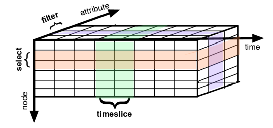
Figure 6: SoN: A set of nodes can be abstracted as a 3 dimensional array with temporal, node and attribute dimensions.

Operators: Below we discuss the important temporal graph algebra operators supported by our system.

1. Selection accepts an SoN or an SoTS along with a boolean function on the nodes or the subgraphs, and returns an SoN or SoTS. Selection performs entity-centric filtering on the operand, and does not alter temporal or attribute dimensions of the data.
   

2. Timeslicing accepts an SoN or an SoTS along with a timepoint (or time interval) $t$, finds the state of each of individual nodes or subgraphs in the operand as of $t$, and returns it as another SoN or SoTS, respectively (SoN/SoTS can represent sets of static nodes or subgraphs as a well). The operator can accept a list of timepoints as input and return a list.
   

3. Graph accepts an SoN and returns an in-memory Graph object containing the nodes in the SoN (with only the edges whose both endpoints are in the SoN). An optional parameter, $t_{p}$, may be specified to get a GraphS valid at time $t_{p}$.
   

4. NodeCompute is analogous to a map operation; it takes as input an SoN (or an SoTS) and a function, and applies the function to all the individual nodes (subgraphs) and returns the results as a set.
   

5. NodeComputeTemporal. Unlike NodeCompute, this operator takes as input a function that operates on a static node (or subgraph) in addition to an SoN (or an SoTS); for each node (subgraph), it returns a sequence of outputs, one for each different state (version) of that node (or subgraph). Optionally, the user may specify another function (NodeComputeDelta) that operates on the delta between two versions of a node (subgraph), which the system can use to compute the output more efficiently. An optional parameter is a method describing points of time at which computation needs to be performed; in the absence of it, the method will be evaluated at all the points of change.
   

6. NodeComputeDelta operator takes as input: (a) a function that operates on a static node (or subgraph) and produces an output quantity, (b) an SoN (or an SoTS) like
   NodeComputeTemporal, (c) a function that operates on the following: a static node (or subgraph), some auxiliary information pertaining to that state of the node (or subgraph), the value of the quantity at that state, and an update (event) to it. This operator returns a sequence of outputs, one for each state of the node (or subgraph), similar to
   NodeComputeTemporal. However, the method of computation in this method is different because it updates the computed quantity for each version incrementally instead of computing it afresh. An optional parameter is the method describing points of time at which to base the comparison. An optional parameter is a method describing points of time at which computation needs to be performed; in the absence of it, the method will be evaluated at all the points of change.
   

7. Compare operator takes as input two SoNs (or two SoTSs) and a scalar function (returning a single value), computes the function value over all the individual components, and returns the differences between the two as a set of (node-id, difference) pairs. This operator tries to abstract the common operation of comparing two different snapshots of a graph at different time points. A simple variation of this operator takes a single SoN (or SoTS) and two timepoints as input, and does the compare on the timeslices of the SoN as of those two timepoints. An optional parameter is the method describing points of time at which to base the comparison.
   

8. Evolution operator samples a specified quantity (provided as a function) over time to return evolution of the quantity over a period of time. An optional parameter is the method describing points of time at which to base the evolution.
   

9. TempAggregation abstractly represents a collection of temporal aggregation operators such as Peak, Saturate, Max, Min, and Mean over a scalar timeseries. The aggregation operations are used over the results of temporal evaluation of a given quantity over an SoN or SoTs. For instance, finding “times at which there was a peak in the network density” is used to find eventful timepoints of high interconnectivity such as conversations in a cellular network, or high transactional activity in a financial network.

5.2 System Implementation

The library is implemented in Python and Java and is built on top of the Spark API. The choice of Spark provides us with an efficient in-memory cluster compute execution platform, circumventing dealing with the issues of data partitioning, communication, synchronization, and fault tolerance. We provide a GraphX integration for utilizing the capabilities of the Spark based graph processing system for static graphs.

The key abstraction in Spark is that of an RDD, which represents a collection of objects of the same type, stored across a cluster. SoN and SoTS are implemented as RDDs of NodeT and SubgraphT respectively (i.e., as RDD<NoteT> and RDD<SubgraphT>). The in-memory graph objects may be implemented using any popular graph representation, specially the ones that support useful libraries on top. We now describe in brief the implementation details for NodeT and SubgraphT, followed by details of the incremental computational operator, and the parallel data fetch operation.

Figure 7 shows sample code snippets for three different analytical tasks – (a) finding the node with the highest clustering coefficient in a historical snapshot; (b) comparing different communities in a network; (c) finding the evolution of network density over a sample of ten points.

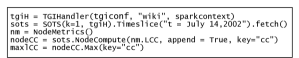
(a) Finding node with highest local clustering coefficient

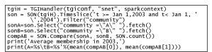
(b) Comparing two communities in a network

(c) Evolution of network density

Figure 7: Examples of analytics using the TAF Python API.

NodeT and SubgraphT: A set of temporal nodes is represented with an RDD of NodeT (temporal node). A temporal node contains the information for a node during a specified time interval. The question of the appropriate physical storage of the NodeT (or SubgraphT) structure is quite similar to storing a temporal graph on disk such as the one using a DeltaGraph or a TGI, however, in-memory instead of disk. Since NodeT is fetched at query time, it is preferable to avoid creating a complicated index, since the cost to create the index at query time is likely to offset any access latency benefits due to the index. An intuitive guess based upon examination of certain temporal analysis tasks is that its access pattern is most likely going to be in a chronological order, i.e., the query requesting the subsequent versions or changes, in order of time. Hence, we store NodeT (and SubgraphT) as an initial snapshot of the node (or subgraph), followed by a list of chronologically sorted events. It provides methods such as GetStartTime(), GetEndTime(), GetStateAt(), GetIterator(), Iter-
ator.GetNextVersion(), Iterator.GetNextEvent(), and so on. We omit the details of these methods as their functionality is apparent from the nomenclature.

NodeComputeDelta: NodeComputeDelta evaluates a quantity over each NodeT (or SubgraphT) using two supplied methods, $f()$ which computes the quantity on a state of the node or subgraph, and, $f_{\Delta}()$, which updates the quantity on a state of the node or subgraph for a given set of event updates. Consider a simple example of finding the fraction of nodes with a specific attribute value in a given SubgraphT. If this were to be performed using
NodeComputeTemporal, the quantity will be computed afresh on each new version of the subgraph, which would cost $\mathcal{O}(N.T)$ operations where $N$ is the size of the operand (number of nodes) and $T$ is the number of versions. However, using the incremental computation, each new version can be processed in constant time after the first snapshot, which adds up to, $\mathcal{O}(N+T)$. While performing the incremental computation, the corresponding $f_{\Delta}()$ method is expected to be defined so as to evaluate the nature of the event – whether it brings about any changing the output quantity or not, i.e., a scalar change value based upon the actual event and the concerned portions of the state of the graph, and also update the auxiliary structure, if used. Code in Figure 8 illustrates the usage of NodeComputeTemporal and NodeComputeDelta in a similar example.

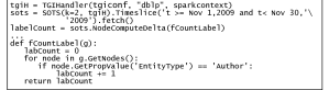
(a) Using NodeComputeTemporal

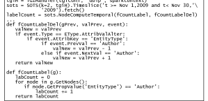
(b) Using NodeComputeDelta

Figure 8: Incremental computation using different methods compute counts of nodes with a specific label in subgraphs over time.

Consider a somewhat more intricate example, where one needs to find counts of a small pattern over time on an SoTS, such as finding the occurrence of a subgraph pattern in the data graph’s history. In order to perform such pattern matching over long sequences of subgraph versions, it is essential to maintain certain inverted indexes which can be looked up to answer in constant time whether an event has caused a change in the answer from a previous state or caused a change in the index itself, or both. Such inverted indexes, quite common to subgraph pattern matching, are required to be updated with every event; otherwise, with every new event update, we would need to look up the new state of the subgraph afresh which would simply reduce it to performing non-indexed subgraph pattern matching over new snapshots of a subgraph at each time point, which is a fairly expensive task. In order to utilize a constantly updated set of indices, the auxiliary information, which is a parameter and a return type for $f_{\Delta}()$, can be utilized. Note that such an incremental computational operator opens up possibilities for using a considerable amount of algorithmic work available in literature on online and streaming graph query evaluation, respectively, to be applied to historical graph analysis. For instance, there is work on pattern matching in streaming [52, 16] and incremental computing [15, 51] contexts, respectively.

Specifying interesting time points: In the map-oriented version operators on an SoN or an SoTS, the time points of evaluation, by default, are all the points of change in the given operand. However, a user may choose to provide a definition of which points to select. This can be as simple as returning a constant set of timepoints, or based on a more complex function of the operand(s). Except the Compare operator, which accepts two operands, other operators allow an optional function, which works on a singe temporal operand; the compare accepts a similar function that operates on two such operands. Two such examples can be seen in Figure 9.

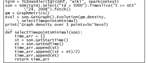
(a) Specifying the start, end and middle point of SON for an Evolution query.

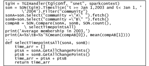
(b) Specifying all change points in two SON’s for a Compare query.

Figure 9: Using the optional timepoint specification function with evolution and comparison queries.

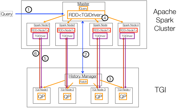
Figure 10: A pictorial representation of the parallel fetch operation between the TGI cluster and the analytics framework cluster. The numbers in circles indicate the relative order of events and the arrowheads indicate the direction of flow.

Data Fetch: In a temporal graph analysis task, we first need to instantiate a TGI connection handler instance. It contains configurations such as address and port of the TGI query manager host, graph-id, and a SparkContext object. Then, a SON (or SOTS) object is instantiated by passing the reference to the TGI handler, and any query specific parameters (such as k-value for fetching 1-hop neighborhoods with SOTS). The next few instructions specify the semantics of the graph to be fetched from the TGI. This is done through the commands explained in Section 5.1, such as the Select, Filter, Timeslice, etc. However, the actual retrieval from the index doesn’t happen until the first statement following the specification instructions. A fetch() command can be used explicitly to tell the system to perform the fetch operation. Upon the fetch() call, the analytics framework sends the combined instructions to the query planner of the TGI, which translates those instructions into an optimal retrieval plan. This prevents the system from retrieving large amounts of data from the index that is a superset of the required information and prune it later.

The analytics engine runs in parallel on a set of machines, so does the graph index. The parallelism at both places speeds up and scales both the tasks. However, if the retrieval graph at the TGI cluster was aggregated at the Query Manager and sent serially to the master of the analytical framework engine after which it was distributed to the different machines on the cluster, it would create a space and time bottleneck at the Query Manager and the master, respectively, for large graphs. In order to bypass this situation, we have designed a parallel fetch operation, in which there is a direct communication between the nodes of the analytics framework cluster and the nodes of the TGI cluster. This happens through a protocol that can be seen in Figure 10. The protocol is briefly described in the following ordered steps:

1. Analytics query containing fetch instructions is received by the TAF master.

2. A handshake between the TAF master and TGI query manager is established. The latter receives fetch instructions and the former is made aware of the active TGI query processor nodes.

3. Parallel fetch starts at the TGI cluster.

4. The TAF master instantiates a TGIDriver instance at each of its cluster machines wrapped in a RDD.

5. Each node at the TAF performs a handshake with one or more of the TGI nodes.

6. Upon completion of fetch at TGI, the individual TGI nodes transfer the SoN to an RDDs on the corresponding TAF nodes.

6 Experimental Evaluation

In this section, we empirically evaluate the efficiency of TGI and TAF. To recap, TGI is a persistent store for entire histories of large graphs, that enables fast retrieval for a diverse set of graph primitives – snapshots, subgraphs, and nodes at past time points or across intervals of time. We primarily highlight the performance of TGI across the entire spectrum of retrieval primitives. We are not aware of a baseline that may compete with TGI across all or a substantial subset of these retrieval primitives. Specialized alternatives such as DeltaGraph for snapshot retrieval is highly unsuitable for node or neighbor version retrieval; a version centric index may be specialized for node-version retrieval but is highly unsuitable for snapshot or neighborhood-version style retrieval. Also note that TGI generalizes all the known approaches including those two; using appropriate parameter configurations, it can even converge to any specific alternative. Secondly, we demonstrate the scalability of TGI design through experiments on parallel fetching for large and varying data sizes. Finally, we also report experiments demonstrating computational scalability of the TAF for a graph analysis task, as well as the benefits of our incremental computational operator.

Datasets and Notation: We use four datasets: (1) Wikipedia citation network consisting of 266,769,613 edge addition events from Jan 2001 to Sept 2010. At its largest point, the graph consists of 21,443,529 nodes and 122,075,026 edges; (2) We augment Dataset 1 by adding around 333 million synthetic events which randomly add new edges or delete existing edges over a period of time, making a total of 700 million events; (3) Similarly, we add 733 million events, making the total around 1 billion events; (4) Using a Friendster gaming network snapshot, we add synthetic dates at uniform intervals to 500 million events with a total of approximately 37.5 million nodes and 500 million edges.

Following key parameters that are varied in the experiments: data store machine count ($m$), replication across dataset ($r$), number of parallel fetching clients ($c$), eventlist size ($l$), snapshot or eventlist partition size ($ps$), and Spark cluster size ($m_{a}$).

We conducted all experiments on an Amazon EC2 cluster. Cassandra ran on machines containing 4 cores and 15GB of available memory. We did not use row caching and the actual memory consumption was much lower that the available limit on those machines. Each fetch client ran on a single core with up to 7.5GB available memory. The machines with TAF nodes running Spark workers ran on a single core and 7.5GB of available memory each.

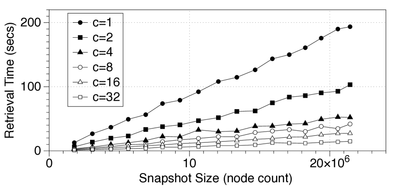
Figure 11: Snapshot retrieval times for varying parallel fetch factor ($c$), on Dataset 1; $m=4$; $r=1,ps=500$.

Snapshot retrieval: Figure 11 shows the snapshot retrieval times for Dataset 1 for different values of the parallel fetch factor, $c$. As we can see, the retrieval cost is directly proportional to the size of the output. Further, using multiple clients to retrieve the snapshots in parallel gives near-linear speedup, especially with low parallelism. This demonstrates that TGI can exploit available parallelism well. We expect that with higher values of $m$ (i.e., if the index were distributed across a larger number of machines), the linear speedup would be seen for larger values of $c$ (this is also corroborated by the next set of experiments). The snapshot retrieval times for dataset 4 can be seen in Figure 13c.

Figure 12 shows snapshot retrieval performance for three different sets of values for $m$ and $r$. We can see that while there is no considerable difference in performance across the different configurations, using two storage machines slightly decreases the query latency over using one machine, in the case of a single query client, $c=1$. For higher $c$ values, we see that $m=2$ has a slight edge over $m=1$. Also, the behavior for the two $m=1$ and $m=2;r=2$ cases are quite similar for same $c$ values. However, we observed that the latter case allows a higher possibility of $c$ value whereas the former peaks out at a lower $c$ value.

Further, the net effect of Cassandra compression for deltas is negligible for TGI. We omit the detailed points of our investigation, but Figure 13a is representative of the general behavior.

Size of the delta partitions (or the number) affects the performance the snapshot retrieval performance only to a small degree as seen in Figure 13b. This occurs due to a the TGI design which makes sure that all the partitions of a delta (micro-deltas) are stored contiguously in a cluster. This demonstrates that TGI is a superset of DeltaGraph where we are able to handle other queries along with efficient snapshot retrieval. Note that we do not provide experimental results on the internals of snapshot retrieval which have been thoroughly explored in our prior work [29].

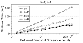
(a) m=1; r=1; ps=500

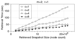
(b) m=2; r=1; ps=500

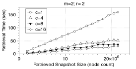
(c) m=2; r=2; ps=500

Figure 12: Snapshot retrieval times across different $m$ and $r$ values on Dataset 1.

(a) Compressed vs. uncompressed delta storage.

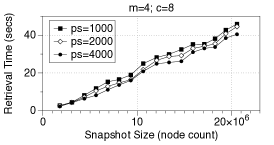
(b) Effect of partition sizes.

(c) Snapshot retrieval times for Dataset 4; $m=6$; $r=1,c=1,ps=500$.

Figure 13: Snapshot retrieval across various parameters.

(a) Effect of eventlist size, $l$.

(b) Speedups due to parallel fetch factor, $c$.

(c) Effect of partition sizes.

Figure 14: Node version retrieval across various parameters.

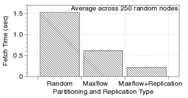
(a)

(b)

(c) TAF computation times for Local Clustering Coefficient on varying graph sizes (N=node count) using different cluster sizes.

Figure 15: Experiments on partitioning type and replication; growing data size; and, TAF analytics computation.

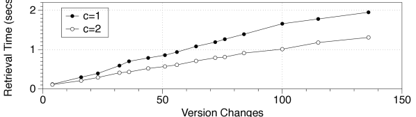
Figure 16: Node version retrieval for Dataset 4; $m=6$; $r=1,c=1,ps=500$.

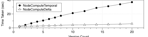
Figure 17: Label counting in several 2-hop neighborhoods through version (NodeComputeTemporal) and incremental (NodeComputeDelta) computation, respectively. We report cumulative time taken (excluding fetch time) over varying version counts; 2 Spark workers were used for dataset 4.

Node History Retrieval: Smaller eventlists or partition sizes provide a lower latency time for retrieving different versions of a node, which can be seen in Figure 14a and Figure 14c, respectively. This is primarily due to the reduction in work required for fetching and deserialization. A higher parallel fetch factor is effective in reducing the latency for version retrieval (Figure 14b). Note that the performance of version retrieval and snapshot retrieval with respect to varying partition sizes is contrary and represents a trade-off. However, smaller eventlist sizes benefit both version retrieval and snapshots. Node version retrieval for Dataset 4 shows a similar behavior, which can be seen in Figure 16.

Neighborhood Retrieval: We compared the performance of retrieving 1-hop neighborhoods, both static and specific versions, using different graph partitioning and replication choices. A topological, flow-based partitioning accesses fewer graph partitions compared to a random partitioning scheme, and a 1-hop neighborhood replication restricts the access to a single partition.This can be seen in Figure 15a for 1-hop neighborhood retrieval latencies. As discussed in Section 4, the 1-hop replication does not affect other queries involving snapshots or individual nodes, as the replicated portion is stored separately from the original partition. In case of a 2-hop neighborhood retrieval, there are similar performance benefits over random partitioning, which can be reasoned based upon similar speed-ups for 1-hop neighborhoods.

Increasing Data Over Time: We observed the fetch performance of TGI with an increasing size of the index. We measured the latencies for retrieving certain snapshots upon varying the time duration of the graph dataset, as shown in Figure 15b. Datasets 2 and 3 contain additional 333 million and 733 million events over dataset 1, respectively. Only a marginal difference in snapshot retrieval performance demonstrates TGI’s scalability for large datasets.

Conducting Scalable Analytics: We examined TAF’s performance through an analytical task for determining the highest local clustering coefficient in historical graph snapshot. Figure 15c shows compute times for the given task on different graph sizes, as well as varying size of the Spark cluster. Speedups due to parallel execution can be observed, especially for larger datasets.

Temporal Computation: Earlier in the chapter, we presented two separate ways of computing a quantity over changing versions of a graph (or node). Those include, evaluating the quantity on different versions of the graph separately, and alternatively, performing it in an incremental fashion, utilizing the result for the previous version and updating it with respect to the graph updates. This can be seen for a simple node label counting task in Figure 8. the benefits due to the incremental (NodeComputeDelta operator) computation over a version-based computation (NodeComputeTemporal operator) can be seen in Figure 17.

7 Conclusion

Graph analytics are increasingly considered crucial in obtaining insights about how interconnected entities behave, how information spreads, what are the most influential entities in the data, and many other characteristics. Analyzing the history of how a graph evolved can provide significant additional insights, especially about the future. Most real-world networks however, are large and highly dynamic. This leads to creation of very large histories, making it challenging to store, query, or analyze them. In this paper, we presented a novel Temporal Graph Index that enables compact storage of very large historical graph traces in a distributed fashion, supporting a wide range of retrieval queries to access and analyze only the required portions of the history. We also present a distributed analytics framework, built on top of Apache Spark, that allows analysts to quickly write complex temporal analysis tasks. Our experiments show that our temporal index exhibits very efficient retrieval performance across a wide range of queries, and can effectively exploit the available parallelism in a distributed setting.

References

- [1] Jans Aasman. Allegro graph: Rdf triple database. Technical report, Franz Incorporated, 2006.
- [2] Jae-wook Ahn, Catherine Plaisant, and Ben Shneiderman. A task taxonomy for network evolution analysis. IEEE Transactions on Visualization and Computer Graphics, 2014.
- [3] L. Arge and J. Vitter. Optimal dynamic interval management in external memory. In FOCS, 1996.
- [4] Sitaram Asur, Srinivasan Parthasarathy, and Duygu Ucar. An event-based framework for characterizing the evolutionary behavior of interaction graphs. ACM TKDD, 2009.
- [5] Bahman Bahmani, Abdur Chowdhury, and Ashish Goel. Fast incremental and personalized pagerank. VLDB, 2010.
- [6] Alain Barrat, Marc Barthelemy, and Alessandro Vespignani. Dynamical processes on complex networks. Cambridge University Press Cambridge, 2008.
- [7] Tanya Y Berger-Wolf and Jared Saia. A framework for analysis of dynamic social networks. In SIGKDD, 2006.
- [8] G. Blankenagel and R. Guting. External segment trees. Algorithmica, 1994.
- [9] A. Bolour, T. L. Anderson, L. J. Dekeyser, and H. K. T. Wong. The role of time in information processing: a survey. SIGMOD, 1982.
- [10] Zhuhua Cai, Dionysios Logothetis, and Georgos Siganos. Facilitating real-time graph mining. In CloudDB, 2012.
- [11] R. Cheng, J. Hong, A. Kyrola, Y. Miao, X. Weng, M. Wu, F. Yang, L. Zhou, F. Zhao, and E. Chen. Kineograph: taking the pulse of a fast-changing and connected world. In EUROSYS, 2012.
- [12] Chris J. Date, Hugh Darwen, and Nikos A. Lorentzos. Temporal data and the relational model. Elsevier, 2002.
- [13] Prasanna Desikan, Nishith Pathak, Jaideep Srivastava, and Vipin Kumar. Incremental page rank computation on evolving graphs. In ACM Special interest tracks and posters of at WWW, 2005.
- [14] David Eisenberg, Edward M Marcotte, Ioannis Xenarios, and Todd O Yeates. Protein function in the post-genomic era. Nature, 2000.
- [15] Wenfei Fan, Xin Wang, and Yinghui Wu. Incremental graph pattern matching. ACM Transactions on Database Systems (TODS), 38(3):18, 2013.
- [16] Jun Gao, Chang Zhou, Jiashuai Zhou, and Jeffrey Xu Yu. Continuous pattern detection over billion-edge graph using distributed framework. In Data Engineering (ICDE), 2014 IEEE 30th International Conference on, pages 556–567. IEEE, 2014.
- [17] B. Gedik and R. Bordawekar. Disk-based management of interaction graphs. TKDE, 2014.
- [18] S. Ghandeharizadeh, R. Hull, and D. Jacobs. Heraclitus: elevating deltas to be first-class citizens in a database programming language. ACM Transactions on Database Systems (TODS), 21(3), 1996.
- [19] A. Ghrab, S. Skhiri, S. Jouili, and E. Zimányi. An analytics-aware conceptual model for evolving graphs. In Data Warehousing and Knowledge Discovery. Springer, 2013.
- [20] Joseph E. Gonzalez, Reynold S. Xin, Ankur Dave, Daniel Crankshaw, Michael J. Franklin, and Ion Stoica. Graphx: Graph processing in a distributed dataflow framework. In OSDI, 2014.
- [21] F. Grandi. T-SPARQL: A TSQL2-like temporal query language for RDF. In ADBIS, 2010.
- [22] D. Greene, D. Doyle, and P. Cunningham. Tracking the evolution of communities in dynamic social networks. In ASONAM, 2010.
- [23] Thilo Gross, Carlos J Dommar D’Lima, and Bernd Blasius. Epidemic dynamics on an adaptive network. Physical review letters, 2006.
- [24] Ranjay Gulati and Martin Gargiulo. Where do interorganizational networks come from? American journal of sociology, 1999.
- [25] W. Hant, Y. Miao, K. Li, M. Wu, F. Yang, L. Zhou, V. Prabhakaran, W. Chen, and E. Chen. Chronos: a graph engine for temporal graph analysis. In EuroSys, 2014.
- [26] H. He and A. Singh. Graphs-at-a-time: query language and access methods for graph databases. In SIGMOD, 2008.
- [27] W. Huo and V. Tsotras. Efficient temporal shortest path queries on evolving social graphs. In SSDBM, 2014.
- [28] U Kang, Hanghang Tong, Jimeng Sun, Ching-Yung Lin, and Christos Faloutsos. Gbase: a scalable and general graph management system. In ACM SIGKDD, 2011.
- [29] Udayan Khurana and Amol Deshpande. Efficient snapshot retrieval over historical graph data. In IEEE ICDE, 2013.
- [30] G. Koloniari and E. Pitoura. Partial view selection for evolving social graphs. In GRADES workshop, 2013.
- [31] A. Kyrola, G. Blelloch, and C. Guestrin. GraphChi: Large-scale graph computation on just a PC. In OSDI, 2012.
- [32] A. Labouseur, J. Birnbaum, Jr. Olsen, P., S. Spillane, J. Vijayan, J. Hwang, and W. Han. The G* graph database: efficiently managing large distributed dynamic graphs. Distributed and Parallel Databases, 2014.
- [33] Kristina Lerman and Rumi Ghosh. Information contagion: An empirical study of the spread of news on digg and twitter social networks. ICWSM, 2010.
- [34] Y. Low, D. Bickson, J. Gonzalez, C. Guestrin, A. Kyrola, and J. Hellerstein. Distributed GraphLab: a framework for machine learning and data mining in the cloud. VLDB, 2012.
- [35] Peter Macko, Virendra J. Marathe, Daniel W. Margo, and Margo I. Seltzer. LLAMA: Efficient Graph Analytics Using Large Multiversioned Arrays . In ICDE, 2015.
- [36] G. Malewicz, M. Austern, A. Bik, J. Dehnert, I. Horn, N. Leiser, and G. Czajkowski. Pregel: a system for large-scale graph processing. In ACM SIGMOD, 2010.
- [37] Youshan Miao, Wentao Han, Kaiwei Li, Ming Wu, Fan Yang, Lidong Zhou, Vijayan Prabhakaran, Enhong Chen, and Wenguang Chen. Immortalgraph: A system for storage and analysis of temporal graphs. ACM TOS, July 2015.
- [38] G. Ozsoyoglu and R.T. Snodgrass. Temporal and real-time databases: a survey. IEEE TKDE, 1995.
- [39] Raj Kumar Pan and Jari Saramäki. Path lengths, correlations, and centrality in temporal networks. Physical Review E, 2011.
- [40] Jorge Pérez, Marcelo Arenas, and Claudio Gutierrez. Semantics and complexity of SPARQL. In The Semantic Web. 2006.
- [41] C. Ren, E. Lo, B. Kao, X. Zhu, and R. Cheng. On querying historial evolving graph sequences. In VLDB, 2011.
- [42] B. Salzberg and V. Tsotras. Comparison of access methods for time-evolving data. ACM Computing Surveys, 1999.
- [43] Bin Shao, Haixun Wang, and Yatao Li. Trinity: A distributed graph engine on a memory cloud. In ACM SIGMOD, 2013.
- [44] R. Snodgrass, editor. The TSQL2 Temporal Query Language. Kluwer, 1995.
- [45] R. Snodgrass and I. Ahn. A taxonomy of time in databases. In SIGMOD, 1985.
- [46] Emad Soroush and Magdalena Balazinska. Time travel in a scientific array database. In IEEE ICDE, 2013.
- [47] Lei Tang, Huan Liu, Jianping Zhang, and Zohreh Nazeri. Community evolution in dynamic multi-mode networks. In SIGKDD, 2008.
- [48] A. Tansel, J. Clifford, S. Gadia, S. Jajodia, A. Segev, and R. Snodgrass (editors). Temporal Databases: Theory, Design, and Implementation. 1993.
- [49] Ian W Taylor, Rune Linding, David Warde-Farley, Yongmei Liu, Catia Pesquita, Daniel Faria, Shelley Bull, Tony Pawson, Quaid Morris, and Jeffrey L Wrana. Dynamic modularity in protein interaction networks predicts breast cancer outcome. Nature biotechnology, 2009.
- [50] V. Tsotras and N. Kangelaris. The snapshot index: an I/O- optimal access method for timeslice queries. Inf. Syst., 1995.
- [51] Gergely Varró, Dániel Varró, and Andy Schürr. Incremental graph pattern matching: Data structures and initial experiments. Electronic Communications of the EASST, 4, 2006.
- [52] Changliang Wang and Lei Chen. Continuous subgraph pattern search over graph streams. In Data Engineering, 2009. ICDE’09. IEEE 25th International Conference on, pages 393–404. IEEE, 2009.
- [53] B. Xuan, A. Ferreira, and A. Jarry. Computing shortest, fastest, and foremost journeys in dynamic networks. International Journal of Foundations of Computer Science, 2003.
- [54] M. Zaharia, M. Chowdhury, M. Franklin, S. Shenker, and I. Stoica. Spark: cluster computing with working sets. In USENIX conference on Hot topics in cloud computing, 2010.