Finding Desirable Objects under Group Categorical Preferences ^⋆

Abstract

Considering a group of users, each specifying individual preferences over categorical attributes, the problem of determining a set of objects that are objectively preferable by all users is challenging on two levels. First, we need to determine the preferable objects based on the categorical preferences for each user, and second we need to reconcile possible conflicts among users’ preferences. A naïve solution would first assign degrees of match between each user and each object, by taking into account all categorical attributes, and then for each object combine these matching degrees across users to compute the total score of an object. Such an approach, however, performs two series of aggregation, among categorical attributes and then across users, which completely obscure and blur individual preferences. Our solution, instead of combining individual matching degrees, is to directly operate on categorical attributes, and define an objective Pareto-based aggregation for group preferences. Building on our interpretation, we tackle two distinct but relevant problems: finding the Pareto-optimal objects, and objectively ranking objects with respect to the group preferences. To increase the efficiency when dealing with categorical attributes, we introduce an elegant transformation of categorical attribute values into numerical values, which exhibits certain nice properties and allows us to use well-known index structures to accelerate the solutions to the two problems. In fact, experiments on real and synthetic data show that our index-based techniques are an order of magnitude faster than baseline approaches, scaling up to millions of objects and thousands of users.

-

1 Introduction

Recommender systems have the general goal of proposing objects (e.g., movies, restaurants, hotels) to a user based on her preferences. Several instances of this generic problem have appeared over the past few years in the Information Retrieval and Database communities; e.g., AT05 ; IBS08 ; BOHG13 ; SKP11 . More recently, there is an increased interest in group recommender systems, which propose objects that are well-aligned with the preferences of a set of users JS07 ; MAS11 ; CC12 ; BC11 . Our work deals with a class of these systems, which we term Group Categorical Preferences (GCP), and has the following characteristics. (1) Objects are described by a set of categorical attributes. (2) User preferences are defined on a subset of the attributes. (3) There are multiple users with distinct, possibly conflicting, preferences. The GCP formulation may appear in several scenarios; for instance, colleagues arranging for a dinner at a restaurant, friends selecting a vacation plan for a holiday break.

Table 1: New York Restaurants

	Attributes
Restaurant	Cuisine	Attire	Place	Price	Parking
$o_{1}$	Eastern	Business casual	Clinton Hill	$$$	Street
$o_{2}$	French	Formal	Time Square	$$$$	Valet
$o_{3}$	Brazilian	Smart Casual	Madison Square	$$	No
$o_{4}$	Mexican	Street wear	Chinatown	$	No

Table 2: User preferences

	Preferences
User	Cuisine	Attire	Place	Price	Parking
$u_{1}$	European	Casual	Brooklyn	$$$	Street
$u_{2}$	French, Chinese	–	–	–	Valet
$u_{3}$	Continental	–	Time Square, Queens	–	–

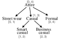
(a) Attire attribute

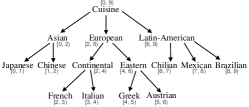
(b) Cuisine attribute

(c) Parking attribute

(d) Place attribute (part of New York places)

Figure 1: Attribute hierarchies

To illustrate GCP, consider the following example. Assume that three friends in New York are looking for a restaurant to arrange a dinner. Suppose that, the three friends are going to use a Web site (e.g., Yelp) in order to search and filter restaurants based on their preferences. Note that in this setting, as well as in other Web-based recommendation systems, categorical description are prevalent compared to numerical attributes. Assume a list of available New York restaurants, shown in Table 1, where each is characterized by five categorical attributes: Cuisine, Attire, Place, Price and Parking. In addition, Figure 1 depicts the hierarchies for these attributes. Attire and Parking are three-level hierarchies, Cuisine and Place are four-level hierarchies, and Price (not shown in Figure 1) is a two-levels hierarchy with four leaf nodes ($\$,...,\$\$\$\$$). Finally, Table 2 shows the three friends’ preferences. For instance, $u_{1}$ prefers European cuisine, likes to wear casual clothes, and prefers a moderately expensive ($\$\$\$$) restaurant in the Brooklyn area offering also street parking. On the other hand, $u_{2}$ likes French and Chinese cuisine, and prefers restaurants offering valet parking, without expressing any preference on attire, price and place.

Observe that if we look at a particular user, it is straightforward to determine his ideal restaurant. For instance, $u_{1}$ clearly prefers $o_{1}$, while $u_{2}$ clearly favors $o_{2}$. These conclusions per user can be reached using the following reasoning. Each preference attribute value $u_{j}.A_{k}$ is matched with the corresponding object attribute value $o_{i}.A_{k}$ using a matching function, e.g., the Jaccard coefficient, and a matching degree per preference attribute is derived. Given these degrees, the next step is to “compose” them into an overall matching degree between a user $u_{j}$ and an object $o_{i}$. Note that several techniques are proposed for “composing” matching degrees; e.g., MAS11 ; JM04 ; K02 ; SKP11 ; C03 . The simplest option is to compute a linear combination, e.g., the sum, of the individual degrees. Finally, alternative aggregations models (e.g., Least-Misery, Most-pleasure, etc.) could also be considered.

Returning to our example, assume that the matching degrees of user $u_{1}$ are: $\langle 1/2,1/2,1/6,1,1\rangle$ for restaurant $o_{1}$, $\langle 1/4,0,0,0,0\rangle$ for $o_{2}$, $\langle 0,1/2,0,0,0\rangle$ for $o_{3}$, and $\langle 0,0,0,0,0\rangle$ for $o_{4}$ (these degrees correspond to Jaccard coefficients computed as explained in Section 3). Note that for almost any “composition” method employed (except those that only, or strongly, consider the Attire attribute), $o_{1}$ is the most favorable restaurant for user $u_{1}$. Using similar reasoning, restaurant $o_{2}$, is ideal for both users $u_{2}$, $u_{3}$.

When all users are taken into consideration, as required by the GCP formulation, several questions arise. Which is the best restaurant that satisfies the entire group? And more importantly, what does it mean to be the best restaurant? A simple answer to the latter, would be the restaurant that has the highest “composite” degree of match to all users. Using a similar method as before, one can define a collective matching degree that “composes” the overall matching degrees for each user. This interpretation, however, enforces an additional level of “composition”, the first being across attributes, and the second across users. These compositions obscure and blur the individual preferences per attribute of each user.

To some extent, the problem at the first “composition” level can be mitigated by requiring each user to manually define an importance weight among his specified attribute preferences. On the other hand, it is not easy, if possible at all, to assign weights to users, so that the assignment is fair. There are two reasons for this. First, users may specify different sets of preference attributes, e.g., $u_{1}$ specifies all five attributes, while $u_{2}$ only Cuisine and Parking. Second, even when considering a particular preference attribute, e.g., Cuisine, users may specify values at different levels of the hierarchy, e.g., $u_{1}$ specifies a European cuisine, while $u_{2}$ French cuisine, which is two levels beneath. Similarly, objects can also have attribute values defined at different levels. Therefore, any “composition” is bound to be unfair, as it may favor users with specific preferences and objects with detailed descriptions, and disfavor users with broader preferences and objects with coarser descriptions. This is an inherent difficulty of the GCP problem.

In this work, we introduce the double Pareto-based aggregation, which provides an objective and fair interpretation to the GCP formulation without “compositing” across preference attributes and users. Under this concept, the matching between a user and an object forms a matching vector. Each coordinate of this vector corresponds to an attribute and takes the value of the corresponding matching degree. The first Pareto-based aggregation is defined over attributes and induces a partial order on these vectors. Intuitively, for a particular user, the first partial order objectively establishes that an object is better, i.e., more preferable, than another, if it is better on all attributes. Then, the second Pareto-based aggregation, defined across users, induces the second and final partial order on objects. According to this order, an object is better than another, if it is more preferable according to all users.

Based on the previous interpretation of the GCP formulation, we seek to solve two distinct problems. The first, which we term the Group-Maximal Categorical Objects (GMCO) problem, is finding the set of maximal, or Pareto-optimal, objects according to the final partial order. Note that since this order is only partial, i.e., two objects may not be comparable, there may exist multiple objects that are maximal; recall, that an object is maximal if there exists no other object that succeeds it in the order considered. In essence, it is the fact that this order is partial that guarantees objectiveness. The GMCO problem has been tackled in our previous work BBS14 .

The second problem, which we term the Group-Ranking Categorical Objects (GRCO) problem, consists of determining an objective ranking of objects. Recall that the double Pareto-based aggregation, which is principal in guaranteeing objectiveness, induces only a partial order on the objects. On the other hand, ranking implies a total order among objects. Therefore, it is impossible to rank objects without introducing additional ordering relationships among objects, which however would sacrifice objectiveness. We address this contradiction, by introducing an objective weak order on objects. Such an order allows objects to share the same tier, i.e., ranked at the same position, but defines a total order among tiers, so that among two tiers, it is always clear which is better.

The GMCO problem has at its core the problem of finding maximal elements according to some partial order. Therefore, it is possible to adapt an existing algorithm to solve the core problem, as we discuss in Section 4.2. While there exists a plethora of main-memory algorithms, e.g., Kung1975 ; Bentley1990 , and more recently of external memory algorithms (termed skyline query processing methods), e.g., BKS01 ; CGGL03 ; PTFS05 , they all suffer from two performance limitations. First, they need to compute the matching degrees and form the matching vectors for all objects, before actually executing the algorithm. Second, it makes little sense to apply index-based methods, which are known to be the most efficient, e.g., the state-of-the-art method of PTFS05 . The reason is that the entries of the index depend on the specific instance, and need to be rebuilt from scratch when the user preferences change, even though the description of objects persists.

To address these limitations, we introduce a novel index-based approach for solving GMCO, which also applies to GRCO. The key idea is to index the set of objects that, unlike the set of matching vectors, remains constant across instances, and defer expensive computation of matching degrees. To achieve this, we apply a simple transformation of the categorical attribute values to intervals, so that each object translates to a rectangle in the Euclidean space. Then, we can employ a space partitioning index, e.g., an R^∗-Tree, to hierarchically group the objects. We emphasize that this transformation and index construction is a one-time process, whose cost is amortized across instances, since the index requires no maintenance, as long as the collection of objects persists. Based on the transformation and the hierarchical grouping, it is possible to efficiently compute upper bounds for the matching degrees for groups of objects. Therefore, for GMCO, we introduce an algorithm that uses these bounds to guide the search towards objects that are more likely to belong to the answer set, avoid computing unnecessary matching degrees.

For the GRCO problem, i.e., finding a (weak) order among objects, there has been a plethora of works on the related topic of combining/fusing multiple ranked lists, e.g., FS93 ; DKNS01 ; AM01 ; MA02 ; FV07 ; MAS11 . However, such methods are not suitable for our GCP formulation. Instead, we take a different approach. We first relax the unanimity in the second Pareto-based aggregation, and require only a percentage $p\%$ of users to agree, resulting in the p-GMCO problem. This introduces a pre-order instead of a partial order, i.e., the induced relation lacks antisymmetry (an object may at the same time be before and after another). Then, building on this notion, we define tiers based on $p$ values, and rank objects according to the tier they belong, which results in an objective weak order. To support the effectiveness of our ranking scheme, we analyze its behaviour in the context of rank aggregation and show that it posseses several desirable theoretical properties.

Contributions. The main contributions of this paper are summarized as follows.

• We introduce and propose an objective and fair interpretation of group categorical preference (GCP) recommender systems, based on double Pareto-based aggregation.

• We introduce three problems in GCP systems, finding the group-maximal objects (GMCO), finding relaxed group-maximal objects ($p$-GMCO), and objectively ranking objects (GRCO).

• We present a method for transforming the hierarchical domain of a categorical attribute into a numerical domain.

• We propose index-based algorithms for all problems, which employ a space partitioning index to hierarchically group objects.

• We theoretically study the behaviour of our ranking scheme and present a number of theoretical properties satisfied by our approach.

• We present several extensions involving the following issues: multi-values attributes, non-tree hierarchies, subspace indexing, and objective attributes.

• We conduct a thorough experimental evaluation using both real and synthetic data.

Outline. The remaining of this paper is organized as follows. Section 3 contains the necessary definitions for the GCP formulation. Then, Section 4 discusses the GMCO problem, Section 5 the $p$-GMCO problem, and Section 6 the GRCO problem. Section 7 discusses various extensions. Section 8 contains a detailed experimental study. Section 2 reviews related work, while Section 9 concludes this paper.

2 Related Work

This section reviews work on recommender systems and algorithms for Pareto aggregation.

2.1 Recommender Systems

There exist several techniques to specify preferences on objects SKP11 ; LL87 . The quantitative preferences, e.g., AW00 ; HKP01 ; KI04 , assign a numeric score to attribute values, signifying importance. For example, values $a$, $b$, $c$ are assigned scores 0.9, 0.7, 0.1, respectively, which implies that $a$ is more preferable than $b$, which in turn is more preferable than $c$. There also exist qualitative preferences, e.g., K02 ; C03 , which are relatively specified using binary relationships. For example, value $a$ is preferred over $b$ and $c$, but $b$, $c$ are indifferent. This work assumes the case of boolean quantitative preferences, where a single attribute value is preferred, while others are indifferent.

The general goal of recommendation systems AT05 ; BOHG13 ; YuHSD14 ; KannanIP14 is to identify those objects that are most aligned to a user’s preferences. Typically, these systems provide a ranking of the objects by aggregating user preferences. Particularly, the work in AW00 defines generic functions that merge quantitative preferences. The works in CBC+00 ; HKP01 deal with linear combinations of preference scores and propose index and view based techniques for ranking tuples. For preferences in general, K02 ; C03 introduce a framework for composing or accumulating interests. Among the discussed methods is the Pareto composition, which is related to the skyline computation, discussed below.

Recently, several methods for group recommendations are proposed JS07 ; MAS11 ; CC12 ; BC11 . These methods, recommend items to a group of users, trying to satisfy all the group members. The existing methods are classified into two approaches. In the first, the preferences of each group member are combined to create a virtual user; the recommendations to the group are proposed w.r.t. to the virtual user. In the second, individual recommendations for each member is computed; the recommendations of all members are merged into a single recommendation. A large number of group recommendation methods have been developed in several domains such as: music SWT08 ; CBH02 ; PiliponyteRK13 ; McCarthyA98 ; ChaoBF05 ; ZXD05 , movies CCKR01 , TV programs JM04 ; YZHG06 ; VKHA09 ; gb02 , restaurants PPC08 ; McCarthy2002 , sightseeing tours GSO11 ; ArdissonoGPST03 ; KW05 , vacation packages McCarthySCMSN06 ; Jameson04 , food ElahiGRMB14 , news PCCA05 , and online communities GXLBHMS10 ; KKYY10 ; BPD08 . Finally, several works study the problem of rank aggregation in the context of group recommendations RACDY10 ; BMR10 ; BF10 ; CMS07 ; NSNK12b .

Several methods to combine different ranked lists are presented in the IR literature. There the data fusion problem is defined. Given a set of ranked lists of documents returned by different search engines, construct a single ranked list combining the individual rankings DKNS01 . Data fusion techniques can be classified based on whether they require knowledge of the relevance scores AM01 . The simplest method based solely on the documents’ ranks is the Borda-fuse model. It assigns as score to each document the summation of its rank in each list. The Condorcet-fuse method MA02 is based on a majoritarian voting algorithm, which specifies that a document $d_{1}$ is ranked higher in the fused list than another document $d_{2}$ if $d_{1}$ is ranked higher than $d_{2}$ more times than $d_{2}$ is ranked higher than $d_{1}$. The approach in FV07 , assumes that a document is ranked better than another if the majority of input rankings is in concordance with this fact and at the same time only a few input rankings refute it. When the relevance scores are available, other fusion techniques, including CombSUM, CombANZ and CombMNZ, can be applied FS93 . In CombSUM, the fused relevance score of a document is the summation of the scores assigned by each source. In CombANZ (resp. CombMNZ), the final score of a document is calculated as that of CombSUM divided (resp. multiplied) by the number of lists in which the document appears.

2.2 Algorithms for Pareto Aggregation

The work of BKS01 rekindled interest in the problem of finding the maximal objects Kung1975 and re-introduces it as the skyline operator. An object is dominated if there exists another object before it according to the partial order enforced by the Pareto-based aggregation. The maximal objects are referred to as the skyline. The authors propose several external memory algorithms. The most well-known method is Block Nested Loops (BNL) BKS01 , which checks each point for dominance against the entire dataset.

The work in CGGL03 observes that examining points according to a monotone (in all attributes) preference function reduces the average number of dominance checks. Based on this fact, the Sort-first Skyline algorithm (SFS) is introduces; including some variations (i.e., LESS GSG07 , and SaLSa BCP08 ) belonging in the class of sort-based skyline algorithms, that improve performance (see BikakisSS14 for more details).

In SLNX09 the multi-pass randomize algorithm RAND is proposed. Initially, RAND selects a random sample; then, multiple passes over the dataset is performed in order to prune points and find the skyline.

In other approaches, multidimensional indexes are used to guide the search for skyline points and prune large parts of the space. The most well-known algorithms is the Branch and Bound Skyline (BBS) method PTFS05 , which uses an R-tree, and is shown to be I/O optimal with respect to this index. Similarly, the Nearest Neighbor algorithm (NN) KRR02 also uses an R-tree performing multiple nearest neighbor searches to identify skyline objects. A bitmap structure is used by Bitmap TEO01 algorithm to encode the input data. In the Index TEO01 algorithm, several B-trees are used to index the data, one per dimension. Other methods, e.g., LZLL07 ; LC10 , employ a space-filling curve, such as the Z-order curve, and use a single-dimensional index. The Lattice Skyline (LS) algorithm MPJ07 builds a specialized data structure for low-cardinality domains.

In partitioning-based approaches, the algorithms divide the initial space into several partitions. The first algorithm in this category, D&C BKS01 computes the skyline objects adopting the divide-and-conquer paradigm. A similar approach with stronger theoretical guarantees is presented in ST12 . Recently, partitioning-based skyline algorithms are proposed in ZMC09 ; JS10 . OSP ZMC09 attempts to reduce the number of checks between incomparable points by recursively partition the skyline points. BSkyTree JS10 enhances ZMC09 by considering both the notions of dominance and incomparability while partitioning the space.

Finally, specific algorithms are proposed to efficiently compute the skyline over partially ordered domains CET05 ; WFP+08 ; SPP09 ; ZMKC10 , metric spaces CL09 , non-metric spaces PDMK09 , or anticorrelated distributions SK13 .

Several lines of research attempt to address the issue that the size of skyline cannot be controlled, by introducing new concepts and/or ranking the skyline (see LB13 for a survey). YM07 ranks tuples based on the number of records they dominate. CJT+06 deals with high-dimensional skylines, and relaxes the notion of dominance to $k$-dominance, according to which a record is $k$-dominated if it is dominated in a subspace of $k$ dimensions. LJZ11 uses a skyline-based partitioning to rank tuples. The $k$ most representative skyline operator is proposed in LYZZ07 , which selects a set of $k$ skyline points, so that the number of points dominated by at least one of them is maximized. In a similar spirit, TDLP09 tries to select the $k$ skyline points that best capture the trade-offs among the parameters. Finally, LYHSB12 attempts to find a small and focused skyline set. The size of the skyline is reduced by asking from users to state additional preferences.

3 Group Categorical Preferences

Table 3 shows the most important symbols and their definition. Consider a set of $d$ categorical attributes $\mathcal{A}=\{A_{1},\dots,$ $A_{d}\}$. The domain of each attribute $A_{k}$ is a hierarchy $\mathcal{H}(A_{k})$. A hierarchy $\mathcal{H}(A_{k})$ defines a tree, where a leaf corresponds to a lowest-level value, and an internal node corresponds to a category, i.e., a set, comprising all values within the subtree rooted at this node. The root of a hierarchy represents the category covering all lowest-level values. We use the symbol $|A_{k}|$ (resp. $|\mathcal{H}(A_{k})|$) to denote the number of leaf (resp. all hierarchy) nodes. With reference to Figure 1, consider the “Cuisine” attribute. The node “Eastern” is a category and is essentially a shorthand for the set $\{$“Greek”, “Austrian”$\}$, since it contains the two leaves, “Greek” and “Austrian”.

Assume a set of objects $\mathcal{O}$. An object $o_{i}\in\mathcal{O}$ is defined over all attributes, and the value of attribute $o_{i}.A_{k}$ is one of the nodes of the hierarchy $\mathcal{H}(A_{k})$. For instance, in Table 1, the value of the “Cuisine” attribute of object $o_{1}$, is the node “Eastern” in the hierarchy of Figure 1.

Table 3: Notation

Symbol	Description
$\mathcal{A}$, $d$	Set of attributes, number of attributes ($|\mathcal{A}|$)
$A_{k}$, $|A_{k}|$	Attribute, number of distinct values in $A_{k}$
$\mathcal{H}(A_{k})$, $|\mathcal{H}(A_{k})|$	Hierarchy of $A_{k}$, number of hierarchy nodes
$\mathcal{O}$, $o_{i}$	Set of objects, an object
$\mathcal{U}$, $u_{j}$	Set of users, a user
$o_{i}.A_{k}$, $u_{j}.A_{k}$	Value of attribute $A_{k}$ in object $o_{i}$, user $u_{j}$
$o_{i}.I_{k}$, $u_{j}.I_{k}$	Interval representation of the value of $A_{k}$ in $o_{i}$, $u_{j}$
$m_{i}^{j}$	Matching vector of object $o_{i}$ to user $u_{j}$
$m_{i}^{j}.A_{k}$	Matching degree of $o_{i}$ to user $u_{j}$ on attribute $A_{k}$
$o_{a}\succ o_{b}$	Object $o_{a}$ is collectively preferred over $o_{b}$
$\mathcal{T}$	The R∗-Tree that indexes the set of objects
$N_{i}$, $e_{i}$	R∗-Tree node, the entry for $N_{i}$ in its parent node
$e_{i}.ptr$, $e_{i}.mbr$	The pointer to node $N_{i}$, the MBR of $N_{i}$
$M_{i}^{j}$	Maximum matching vector of entry $e_{i}$ to user $u_{j}$
$M_{i}^{j}.A_{k}$	Maximum matching degree of $e_{i}$ to user $u_{j}$ on $A_{k}$

Further, assume a set of users $\mathcal{U}$. A user $u_{i}\in\mathcal{U}$ is defined over a subset of the attributes, and for each specified attribute $u_{i}.A_{j}$, its value in one of the hierarchy $\mathcal{H}(A_{j})$ nodes. For all unspecified attributes, we say that user $u_{i}$ is indifferent to them. Note that, an object (resp. a user) may has (resp. specify) multiple values for each attribute (see Section 7.1).

Given an object $o_{i}$, a user $u_{j}$, and a specified attribute $A_{k}$, the matching degree of $o_{i}$ to $u_{j}$ with respect to $A_{k}$, denoted as $m_{i}^{j}.A_{k}$, is specified by a matching function $\textbf{M}\colon dom(A_{k})\times dom(A_{k})\to[0,1]$. The matching function defines the relation between the user’s preferences and the objects attribute values. For an indifferent attribute $A_{k}$ of a user $u_{j}$, we define $m_{i}^{j}.A_{k}=1$.

Note that, different matching functions can be defined per attribute and user; for ease of presentation, we assume a single matching function. Moreover, note that this function can be any user defined function operating on the cardinalities of intersections and unions of hierarchy attributes. For example, it can be the Jaccard coefficient, i.e., $m_{i}^{j}.A_{k}=\frac{|o_{i}.A_{k}\cap u_{j}.A_{k}|}{|o_{i}.A_{k}\cup u_{j}.A_{k}|}$. The numerator counts the number of leaves in the intersection, while the denominator counts the number of leaves in the union, of the categories $o_{i}.A_{k}$ and $u_{j}.A_{k}$. Other popular choices are the Overlap coefficient: $\frac{|o_{i}.A_{k}\cap u_{j}.A_{k}|}{\min{(|o_{i}.A_{k}|,|u_{j}.A_{k}|)}}$, and the Dice coefficient: $2\frac{|o_{i}.A_{k}\cap u_{j}.A_{k}|}{|o_{i}.A_{k}|+|u_{j}.A_{k}|}$.

In our running example, we assume the Jaccard coefficient. Hence, the matching degree of restaurant $o_{1}$ to user $u_{1}$ w.r.t. “Attire” is $\frac{|\text{``Business casual''}\cap\text{``Casual''}|}{|\text{``Business casual''}\cup\text{``Casual''}|}=$ $\frac{|\{\text{``Business casual''}\}|}{|\{\text{``Business casual''},\text{``Smart casual''}|}=\frac{1}{2}$, where we substituted “Casual” with the set $\{$“Business casual”, “Smart casual”$\}$.

Table 4: Matching vectors

	User
Restaurant	$u_{1}$	$u_{2}$	$u_{3}$
$o_{1}$	$\langle 1/2,1/2,1/6,1,1\rangle$	$\langle 0,1,1,1,0\rangle$	$\langle 0,1,0,1,1\rangle$
$o_{2}$	$\langle 1/4,0,0,0,0\rangle$	$\langle 1,1,1,1,1\rangle$	$\langle 1/2,1,1,1,1\rangle$
$o_{3}$	$\langle 0,1/2,0,0,0\rangle$	$\langle 0,1,1,1,0\rangle$	$\langle 0,1,0,1,1\rangle$
$o_{4}$	$\langle 0,0,0,0,0\rangle$	$\langle 0,1,1,1,0\rangle$	$\langle 0,1,0,1,1\rangle$

Given an object $o_{i}$ and a user $u_{j}$, the matching vector of $o_{i}$ to $u_{j}$, denoted as $m_{i}^{j}$, is a $d$-dimensional point in $[0,1]^{d}$, where its $k$-th coordinate is the matching degree with respect to attribute $A_{k}$. Furthermore, we define the norm of the matching vector to be $\|m_{i}^{j}\|=\sum_{A_{k}\in\mathcal{A}}m_{i}^{j}.A_{k}$. In our example, the matching vector of restaurant $o_{1}$ to user $u_{1}$ is $\langle 1/2,1/2,1/6,1,1\rangle$. All matching vectors of this example are shown in Table 4.

4 The Group-Maximal Categorical Objects (GMCO) Problem

Section 4.1 introduces the GMCO problem, and Section 4.2 describes a straightforward baseline approach. Then, Section 4.3 explains a method to convert categorical values into intervals, and Section 4.4 introduces our proposed index-based solution.

4.1 Problem Definition

We first consider a particular user $u_{j}$ and examine the matching vectors. The first Pareto-based aggregation across the attributes of the matching vectors, induces the following partial and strict partial “preferred” orders on objects. An object $o_{a}$ is preferred over $o_{b}$, for user $u_{j}$, denoted as $o_{a}\succeq^{j}o_{b}$ iff for every specified attribute $A_{k}$ of the user it holds that $m_{a}^{j}.A_{k}\geq m_{b}^{j}.A_{k}$. Moreover, object $o_{a}$ is strictly preferred over $o_{b}$, for user $u_{j}$, denoted as $o_{a}\succ^{j}o_{b}$ iff $o_{a}$ is preferred over $o_{b}$ and additionally there exists a specified attribute $A_{k}$ such that ${m_{a}^{j}.A_{k}>m_{b}^{j}.A_{k}}$. Returning to our example, consider user $u_{1}$ and its matching vector $\langle 0,1/2,0,0,0\rangle$ for $o_{3}$, and $\langle 0,0,0,0,0\rangle$ for $o_{4}$. Observe that $o_{3}$ is strictly preferred over $o_{4}$.

We now consider all users in $\mathcal{U}$. The second Pareto-based aggregation across users, induces the following strict partial “collectively preferred” order on objects. An object $o_{a}$ is collectively preferred over $o_{b}$, if $o_{a}$ is preferred over $o_{b}$ for all users, and there exists a user $u_{j}$ for which $o_{a}$ is strictly preferred over $o_{b}$. From Table 4, it is easy to see that restaurant $o_{1}$ is collectively preferred over $o_{3}$, because $o_{1}$ is preferred by all three users, and strictly preferred by user $u_{1}$.

Given the two Pareto-based aggregations, we define the collectively maximal objects in $\mathcal{O}$ with respect to users $\mathcal{U}$, as the set of objects for which there exists no other object that is collectively preferred over them. In our running example, $o_{1}$ and $o_{2}$ objects are both collectively preferred over $o_{3}$ and $o_{4}$. There exists no object which is collectively preferred over $o_{1}$ and $o_{2}$, and thus are the collectively maximal objects. We next formally define the GMCO problem.

Problem 1. [GMCO] Given a set of objects $\mathcal{O}$ and a set of users $\mathcal{U}$ defined over a set of categorical attributes $\mathcal{A}$, the Group-Maximal Categorical Objects (GMCO) problem is to find the collectively maximal objects of $\mathcal{O}$ with respect to $\mathcal{U}$.

4.2 A Baseline Algorithm (BSL)

The GMCO problem can be transformed to a maximal elements problem, or a skyline query, where the input elements are the matching vectors. Note, however, that the GMCO problem is different than computing the conventional skyline, i.e., over the object’s attribute values.

The Baseline (BSL) method, whose pseudocode is depicted in Algorithm 1, takes advantage of this observation. The basic idea of BSL is for each object $o_{i}$ (loop in line 1) and for all users (loop in line 2), to compute the matching vectors $m_{i}^{j}$ (line 3). Subsequently, BSL constructs a $|\mathcal{U}|$-dimensional tuple $r_{i}$ (line 4), so that its $j$-th entry is a composite value equal to the matching vector $m_{i}^{j}$ of object $o_{i}$ to user $u_{j}$. When all users are examined, tuple $r_{i}$ is inserted in the set $\mathcal{R}$ (line 5).

The next step is to find the maximal elements, i.e., compute the skyline over the records in $\mathcal{R}$. It is easy to prove that tuple $r_{i}$ is in the skyline of $\mathcal{R}$ iff object $o_{i}$ is a collectively maximally preferred object of $\mathcal{O}$ w.r.t. $\mathcal{U}$. Notice, however, that due to the two Pareto-based aggregations, each attribute of a record $r_{i}\in\mathcal{R}$ is also a record that corresponds to a matching vector, and thus is partially ordered according to the preferred orders defined in Section 3. Therefore, in order to compute the skyline of $\mathcal{R}$, we need to apply a skyline algorithm (line 6), such as BKS01 ; PTFS05 ; GSG07 .

Computational Complexity. The computational cost of BSL is the sum of two parts. The first is computing the matching degrees, which takes $O(|\mathcal{O}|\cdot|\mathcal{U}|)$ time. The second is computing the skyline, which requires ${O(|\mathcal{O}|^{2}\cdot|\mathcal{U}|\cdot d)}$ comparisons, assuming a quadratic time skyline algorithms is used. Therefore, BSL takes $O(|\mathcal{O}|^{2}\cdot|\mathcal{U}|\cdot d)$ time.

Input: objects $\mathcal{O}$, users $\mathcal{U}$

Output: $CM$ the collectively maximal

Variables: $\mathcal{R}$ set of intermediate records

1 foreach $o_{i}\in\mathcal{O}$ do

2       foreach $u_{j}\in\mathcal{U}$ do

3             compute $m_{i}^{j}$

4             $r_{i}[j]\leftarrow m_{i}^{j}$

5            

6      insert $r_{i}$ into $\mathcal{R}$

7      

8$CM\leftarrow$ SkylineAlgo ($\mathcal{R}$)

Algorithm 1 BSL

4.3 Hierarchy Transformation

This section presents a simple method to transform the hierarchical domain of a categorical attribute into a numerical domain. The rationale is that numerical domains can be ordered, and thus tuples can be stored in multidimensional index structures. The index-based algorithm of Section 4.4 takes advantage of this transformation.

Consider an attribute $A$ and its hierarchy $\mathcal{H}(A)$, which forms a tree. We assume that any internal node has at least two children; if a node has only one child, then this node and its child are treated as a single node. Furthermore, we assume that there exists an ordering, e.g., the lexicographic, among the children of any node that totally orders all leaf nodes.

The hierarchy transformation assigns an interval to each node, similar to labeling schemes such as ABJ89 . The $i$-th leaf of the hierarchy (according to the ordering) is assigned the interval $[i-1,i)$. Then, each internal node is assigned the smallest interval that covers the intervals of its children. Figure 1 depicts the assigned intervals for all nodes in the two car hierarchies.

Following this transformation, the value on the $A_{k}$ attribute of an object $o_{i}$ becomes an interval $o_{i}.I_{k}=[o_{i}.I_{k}^{-},o_{i}.I_{k}^{+})$. The same holds for a user $u_{j}$. Therefore, the transformation translates the hierarchy $H(A_{k})$ into the numerical domain $[0,|A_{k}|]$.

An important property of the transformation is that it becomes easy to compute matching degrees for metrics that are functions on the cardinalities of intersections or unions of hierarchy attributes. This is due to the following properties, which use the following notation: for a closed-open interval $I=[\alpha,\beta)$, define $\|I\|=\beta-\alpha$.

Proposition 1. For objects/users $x$, $y$, and an attribute $A_{k}$, let $x.I_{k}$, $y.I_{k}$ denote the intervals associated with the value of $x$, $y$ on $A_{k}$. Then the following hold:

1. $|x.A_{k}|=\|x.I_{k}\|$

2. $|x.A_{k}\cap y.A_{k}|=\|x.I_{k}\cap y.I_{k}\|$

3. $|x.A_{k}\cup y.A_{k}|=\|x.I_{k}\|+\|y.I_{k}\|-\|x.I_{k}\cap y.I_{k}\|$

Proof. For a leaf value $x.A_{k}$, it holds that $|x.A_{k}|=1$. By construction of the transformation, $\|x.I_{k}\|=1$. For a non-leaf value $x.A_{k}$, $|x.A_{k}|$ is equal to the number of leaves under $x.A_{k}$. Again, by construction of the transformation, $\|x.I_{k}\|$ is equal to the smallest interval that covers the intervals of the leaves under $x.A_{k}$, and hence equal to $|x.A_{k}|$. Therefore for any hierarchy value, it holds that $x.A_{k}=\|x.I_{k}\|$.

Then, the last two properties trivially follow. The third holds since ${|x.A_{k}\cup y.A_{k}|=}$ $|x.A_{k}|+|y.A_{k}|-|x.A_{k}\cap y.A_{k}|$. ◻

4.4 An Index-based Algorithm (IND)

This section introduces the Index-based GMCO (IND) algorithm. The key ideas of IND are: (1) apply the hierarchy transformation, previously described, and index the resulting intervals, and (2) define upper bounds for the matching degrees of a group of objects, so as to guide the search and quickly prune unpromising objects.

We assume that the set of objects $\mathcal{O}$ and the set of users $\mathcal{U}$ are transformed so that each attribute $A_{k}$ value is an interval $I_{k}$. Therefore, each object (and user) defines a (hyper-)rectangle on the $d$-dimensional cartesian product of the numerical domains, i.e., $[0,|A_{1}|)\times\dots\times[0,|A_{d}|)$.

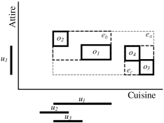
Figure 2: Transformed objects and users

Figure 2 depicts the transformation of the objects and users shown in Tables 1 & 2, considering only the attributes Cuisine and Attire. For instance, object $o_{1}$ is represented as the rectangle $[4,6)\times[2,3)$ in the “Cuisine”$\times$“Attire” plane. Similarly, user $u_{1}$ is represented as two intervals, $[2,6)$, $[1,3)$, on the transformed “Cuisine”, “Attire” axes, respectively.

The IND algorithm indexes the set of objects in this $d$-dimensional space. In particular, IND employs an R^∗-Tree $\mathcal{T}$ BKSS90 , which is well suited to index rectangles. Each $\mathcal{T}$ node corresponds to a disk page, and contains a number of entries. Each entry $e_{i}$ comprises (1) a pointer $e_{i}.ptr$, and (2) a Minimum Bounding Rectangle (MBR) $e_{i}.mbr$. A leaf entry $e_{i}$ corresponds to an object $o_{i}$, its pointer $o_{i}.ptr$ is null, and $e_{i}.mbr$ is the rectangle defined by the intervals of $o_{i}$. A non-leaf entry $e_{i}$ corresponds to a child node $N_{i}$, its pointer $e_{i}.ptr$ contains the address of $N_{i}$, and $e_{i}.mbr$ is the MBR of (i.e., the tightest rectangle that encloses) the MBRs of the entries in $N_{i}$.

Due to its enclosing property, the MBR of an entry $e_{i}$ encloses all objects that are stored at the leaf nodes within the $\mathcal{T}$ subtree rooted at node $N_{i}$. It is often helpful to associate an entry $e_{i}$ with all the objects it encloses, and thus treat $e_{i}$ as a group of objects.

Consider a $\mathcal{T}$ entry $e_{i}$ and a user $u_{j}\in\mathcal{U}$. Given only the information within entry $e_{i}$, i.e., its MBR, and not the contents, i.e., its enclosing objects, at the subtree rooted at $N_{i}$, it is impossible to compute the matching vectors for the objects within this subtree. However, it is possible to derive an upper bound for the matching degrees of any of these objects.

We define the maximum matching degree $M_{i}^{j}.A_{k}$ of entry $e_{i}$ on user $u_{j}$ w.r.t. specified attribute $A_{k}$ as the highest attainable matching degree of any object that may reside within $e_{i}.mbr$. To do this we first need a way to compute lower and upper bounds on unions and intersections of a user interval with an MBR.

Proposition 2. Fix an attribute $A_{k}$. Consider an object/user $x$, and let $I_{x}$, denote the interval associated with its value on $A_{k}$. Also, consider another object/user $y$ whose interval $I_{y}$ on $A_{k}$ is contained within a range $R_{y}$. Given an interval $I$, $\delta(I)$ returns $0$ if $I$ is empty, and $1$ otherwise. Then the following hold:

1. $1\ \leq|y.A_{k}|\leq\|R_{y}\|$

2. $\delta(I_{x}\cap R_{y})\ \leq|x.A_{k}\cap y.A_{k}|\leq\|I_{x}\cap R_{y}\|$

3. $\|I_{x}\|+1-\delta(I_{x}\cap R_{y})\ \leq|x.A_{k}\cup y.A_{k}|\leq\|I_{x}\|+\|R_{y}\|-\delta(I_{x}\cap R_{y})$

Proof. Note that for the object/user $y$ with interval $I_{y}$ on $A_{k}$, it holds that $I_{y}\subseteq R_{y}$.

(1) For the left inequality of the first property, observe that value $y.A_{k}$ is a node that contains at least one leaf, hence $1\leq|y.A_{k}|$. Furthermore, for the right inequality, $|y.A_{k}|=\|I_{y}\|\leq\|R_{y}\|$.

(2) For the left inequality of the second property, observe that the value ${x.A_{k}\cap y.A_{k}}$ contains either at least one leaf when the intersection is not empty, and no leaf otherwise. The right inequality follows from the fact that ${I_{x}\cap I_{y}\subseteq I_{x}\cap R_{y}}$.

(3) For the left inequality of the third property, assume first that $I_{x}\cap I_{y}=\varnothing$; hence $\delta(I_{x}\cap R_{y})=0$. In this case, it holds that $\|I_{x}\cup I_{y}\|=\|I_{x}\|+\|I_{y}\|$. By the first property, we obtain $1\leq\|I_{y}\|$. Combining the three relations, we obtain the left inequality. Now, assume that $I_{x}\cap I_{y}\neq\varnothing$; hence $\delta(I_{x}\cap R_{y})=1$. In this case, it also holds that $\|I_{x}\|\leq\|I_{x}\cup I_{y}\|$, and the left inequality follows.

For the right inequality of the third property, observe that $\|I_{x}\cup I_{y}\|=$ ${\|I_{x}\|+\|I_{y}\|-\|I_{x}\cap I_{y}\|}$. By the first property, we obtain $\|I_{y}\|\leq\|R_{y}\|$, and ${-\|I_{x}\cap I_{y}\|}$ $\leq-\delta(I_{x}\cap R_{y})$, by the second. The right inequality follows from combining these three relations. ◻

Then, defining the maximum matching degree reduces to appropriately selecting the lower/upper bounds for the specific matching function used. For example, consider the case of the Jaccard coefficient, $\frac{|o_{i}.A_{k}\cap u_{j}.A_{k}|}{|o_{i}.A_{k}\cup u_{j}.A_{k}|}$. Assume $e_{i}$ is a non-leaf entry, and let $e_{i}.R_{k}$ denote the range of the MBR on the $A_{k}$ attribute. We also assume that $u_{j}.I_{k}$ and $e_{i}.R_{k}$ overlap. Then, we define $M_{i}^{j}.A_{k}=\frac{\|e_{i}.R_{k}\cap u_{j}.I_{k}\|}{\|u_{j}.I_{k}\|}$, where we have used the upper bound for the intersection in the enumerator and the lower bound for the union in the denominator, according to Figure 2. For an indifferent to the user attribute $A_{k}$, we define $M_{i}^{j}.A_{k}=1$. Now, assume that $e_{i}$ is a leaf entry, that corresponds to object $o_{i}$. Then the maximum matching degree $M_{i}^{j}.A_{k}$ is equal to the matching degree $m_{i}^{j}.A_{k}$ of $o_{i}$ to $u_{j}$ w.r.t. $A_{k}$.

Computing maximum matching degrees for other metrics is straightforward. In any case, the next lemma shows that an appropriately defined maximum matching degree is an upper bound to the matching degrees of all objects enclosed in entry $e_{i}$.

Proposition 3. The maximum matching degree $M_{i}^{j}.A_{k}$ of entry $e_{i}$ on user $u_{j}$ w.r.t. specified attribute $A_{k}$ is an upper bound to the highest matching degree in the group that $e_{i}$ defines.

Proof. The maximum matching degree is an upper bound from Figure 2. ◻

In analogy to the matching vector, the maximum matching vector $M_{i}^{j}$ of entry $e_{i}$ on user $u_{j}$ is defined as a $d$-dimensional vector whose $k$-th coordinate is the maximum matching degree $M_{i}^{j}.A_{k}$. Moreover, the norm of the maximum matching vector is $\|M_{i}^{j}\|=\sum_{A_{k}\in\mathcal{A}}M_{i}^{j}.A_{k}$.

Next, consider a $\mathcal{T}$ entry $e_{i}$ and the entire set of users $\mathcal{U}$. We define the score of an entry $e_{i}$ as $score(e_{i})=\sum_{u_{j}\in\mathcal{U}}\|M_{i}^{j}\|$. This score quantifies how well the enclosed objects of $e_{i}$ match against all users’ preferences. Clearly, the higher the score, the more likely that $e_{i}$ contains objects that are good matches to users.

Input: R^∗-Tree $\mathcal{T}$, users $\mathcal{U}$

Output: $CM$ the collectively maximal

Variables: $H$ a heap with $\mathcal{T}$ entries sorted by $score()$

1 $CM\leftarrow\varnothing$

2 read $\mathcal{T}$ root node

3 insert in $H$ the root entries

4 while $H$ is not empty do

5       $e_{x}\leftarrow$ pop $H$

6       if $e_{x}$ is non-leaf then

7             $N_{x}\leftarrow$ read node $e_{x}.ptr$

8             foreach $e_{i}\in N_{x}$ do

9                   $pruned\leftarrow false$

10                   foreach $u_{j}\in\mathcal{U}$ do

11                         compute $M_{i}^{j}$

12                        

13                  foreach $o_{a}\in CM$ do

14                         if $\forall A_{j}\!:m_{a}^{j}\!\succeq\!M_{i}^{j}\land\exists A_{k}\!:m_{a}^{k}\!\succ\!M_{i}^{k}$ then

15                               $pruned\leftarrow true$

16                               break

17                              

18                        

19                  if not $pruned$ then

20                         insert $e_{i}$ in $H$

21                        

22                  

23            

24      else

25             $o_{x}\leftarrow e_{x}$

26             $result\leftarrow true$

27             foreach $o_{a}\in CM$ do

28                   if $o_{a}\succ o_{x}$ then

29                         $result\leftarrow false$

30                         break

31                        

32                  

33            if $result$ then

34                   insert $o_{x}$ in $CM$

35                  

36            

37      

Algorithm 2 IND

Algorithm Description. Algorithm 2 presents the pseudocode for IND. The algorithm maintains two data structures: a heap $H$ which stores $\mathcal{T}$ entries sorted by their score, and a list $CM$ of collectively maximal objects discovered so far. Initially the list $CM$ is empty (line 1), and the root node of the R^∗-Tree is read (line 2). The score of each root entry is computed and all entries are inserted in $H$ (line 3). Then, the following process (loop in line 4) is repeated as long as $H$ has entries.

The $H$ entry with the highest score, say $e_{x}$, is popped (line 5). If $e_{x}$ is a non-leaf entry (line 6), it is expanded, which means that the node $N_{x}$ identified by $e_{x}.ptr$ is read (line 7). For each child entry $e_{i}$ of $N_{x}$ (line 8), its maximum matching degree $M_{i}^{j}$ with respect to every user $u_{j}\in\mathcal{U}$ is computed (lines 10–11). Then, the list $CM$ is scanned (loop in line 12). If there exists an object $o_{a}$ in $CM$ such that (1) for each user $u_{j}$, the matching vector $m_{a}^{j}$ of $o_{a}$ is better than $M_{i}^{j}$, and (2) there exists a user $u_{k}$ so that the matching vector $m_{a}^{k}$ of $o_{a}$ is strictly better than $M_{i}^{k}$, then entry $e_{i}$ is discarded (lines 13–15). It is straightforward to see (from Figure 2) that if this condition holds, $e_{i}$ cannot contain any object that is in the collectively maximal objects, which guarantees IND’ correctness. When the condition described does not hold (line 16), the score of $e_{i}$ is computed and $e_{i}$ is inserted in $H$ (line 17).

Now, consider the case that $e_{x}$ is a leaf entry (line 18), corresponding to object $o_{x}$ (line 19). The list $CM$ is scanned (loop in line 21). If there exists an object that is collectively preferred over $o_{x}$ (line 22), it is discarded. Otherwise (line 25–26), $o_{x}$ is inserted in $CM$.

The algorithm terminates when $H$ is empty (loop in line 4), at which time the list $CM$ contains the collectively maximal objects.

Computational Analysis. IND performs object to object comparisons as well as object to non-leaf entries. Since there are at most $|\mathcal{O}|$ non-leaf entries, IND performs $O(|\mathcal{O}|^{2}\cdot|\mathcal{U}|\cdot d)$ comparisons in the worst case. Further it computes matching degrees on the fly at a cost of $O(|\mathcal{O}|\cdot|\mathcal{U}|)$. Overall, IND takes ${O(|\mathcal{O}|^{2}\cdot|\mathcal{U}|\cdot d)}$ time, the same as BSL. However, in practice IND is more than an order of magnitude faster than BSL (see Section 8).

Example. We demonstrate IND, using our running example, as depicted in Figure 2. The four objects are indexed by an R^∗-Tree, whose nodes are drawn as dashed rectangles. Objects $o_{1}$, $o_{2}$ are grouped in entry $e_{b}$, while $o_{3}$, $o_{4}$ in entry $e_{c}$. Entries $e_{b}$ and $e_{c}$ are the entries of the root $e_{a}$. Initially, the heap contains the two root entries, $H=\{e_{b},e_{c}\}$. Entry $e_{b}$ has the highest score (the norm of its maximum matching vector is the largest), and is thus popped. The two child entries $o_{1}$ and $o_{2}$ are obtained. Since the list $CM$ is empty, no child entry is pruned and both are inserted in the heap, which becomes $H=\{o_{1},o_{2},e_{c}\}$. In the next iteration, $o_{2}$ has the highest score and is popped. Since this is a leaf entry, i.e., an object, and $CM$ is empty, $o_{2}$ is inserted in the result list, $CM=\{o_{2}\}$. Subsequently, $o_{1}$ is popped and since $o_{2}$ is not collectively preferred over it, $o_{1}$ is also placed in the result list, $CM=\{o_{2},o_{1}\}$. In the final iteration, entry $e_{c}$ is popped, but the objects in $CM$ are collectively preferred over both $e_{c}$ child. Algorithm IND concludes, finding the collectively maximal $CM=\{o_{2},o_{1}\}$.

5 The p-Group-Maximal Categorical Objects (p-GMCO) Problem

Section 5.1 introduces the $p$-GMCO problem, and Section 5.2 presents an adaptation of the BSL method, while Section 5.3 introduces an index-based approach.

5.1 Problem Definition

As the number of users increases, it becomes more likely that the users express very different and conflicting preferences. Hence, it becomes difficult to find a pair of objects such that the users unanimously agree that one is worst than the other. Ultimately, the number of maximally preferred objects increases. This means that the answer to an GMCO problem with a large set of users becomes less meaningful.

The root cause of this problem is that we require unanimity in deciding whether an object is collectively preferred by the set of users. The following definition relaxes this requirement. An object $o_{a}$ is $p$-collectively preferred over $o_{b}$, denoted as $o_{a}\succ_{p}o_{b}$, iff there exist a subset $\mathcal{U}_{p}\subseteq\mathcal{U}$ of at least $\lceil\frac{p}{100}\cdot|\mathcal{U}|\rceil$ users such that for each user $u_{i}\in\mathcal{U}_{p}$ $o_{a}$ is preferred over $o_{b}$, and there exists a user $u_{j}\in\mathcal{U}_{p}$ for which $o_{a}$ is strictly preferred over $o_{b}$. In other words, we require only $p\%$ of the users votes to decide whether an object is universally preferred. Similarly, the $p$-collectively maximal objects of $\mathcal{O}$ with respect to users $\mathcal{U}$, is defined as the set of objects in $\mathcal{O}$ for which there exists no other object that is $p$-collectively preferred over them. The above definitions give rise to the $p$-GMCO problem.

Problem 2. [$p$-GMCO] Given a set of objects $\mathcal{O}$ and a set of users $\mathcal{U}$ defined over a set of categorical attributes $\mathcal{A}$, the $p$-Group-Maximal Categorical Objects ($p$-GMCO) problem is to find the $p$-collectively maximal objects of $\mathcal{O}$ with respect to $\mathcal{U}$.

Following the definitions, we can make a number of important observations, similar to those in the $k$-dominance notion CJT+06 . First, if an object is collectively preferred over some other object, it is also $p$-collectively preferred over that same object for any $p$. As a result, an object that is $p$-collectively maximal is also collectively maximal for any $p$. In other words, the answer to the $p$-GMCO problem is a subset of the answer to the corresponding GMCO.

Second, consider an object $o$ that is not $p$-collectively maximal. Note that it is possible that no $p$-collectively maximal object is $p$-collectively preferred over $o$. As a result checking if $o$ is a result by considering only the $p$-collectively maximal objects may lead to false positives. Fortunately, it holds that there must exist a collectively maximal object that is $p$-collectively preferred over $o$. So it suffices to check $o$ against the collectively maximal objects only (and not just the subset that is $p$-collectively maximal).

Example. Consider the example in Tables 1 & 2. If we consider $p=100$, we require all users to agree if an object is collectively preferred. So, the $100$-collectively maximal objects are the same as the collectively maximal objects (i.e., $o_{1}$, $o_{2}$). Let’s assume that $p=60$; i.e., $\lceil\frac{60}{100}\cdot 3\rceil=2$ users. In this case, only the restaurant $o_{2}$ is $60$-collectively maximal, since, $o_{2}$ is $60$-collectively preferred over $o_{1}$, if we consider the set of users $u_{2}$ and $u_{3}$. Finally, if $p=30$, we consider only one user in order to decide if an object is collectively preferred. In this case, the $30$-collectively maximal is an empty set, since $o_{2}$ is $30$-collectively preferred over $o_{1}$, if we consider either user $u_{2}$ or $u_{3}$, and also $o_{1}$ is $30$-collectively preferred over $o_{2}$, if we consider user $u_{1}$.

Input: objects $\mathcal{O}$, users $\mathcal{U}$

Output: $p$-$CM$ the $p$-collectively maximal

Variables: $CM$ the collectively maximal

$\vdots$

7 foreach $o_{i}\in CM$ do

      8 $inpCM\leftarrow true$

      9 foreach $o_{j}\in CM\backslash o_{i}$  do

            10 if $o_{j}\succ_{p}o_{i}$ then

                  11 $inpCM\leftarrow false$

                  12 break;

            

      13if $inpCM$ then

            14 insert $o_{i}$ to $p\text{-}CM$

            

      

Algorithm 3 $p$-BSL

5.2 A Baseline Algorithm (p-BSL)

Based on the above observations, we describe a baseline algorithm for the $p$-GMCO problem, based on BSL. Algorithm 3 shows the changes with respect to the BSL algorithm; all omitted lines are identical to those in Algorithm 1. The $p$-BSL algorithm first computes the collectively maximal objects applying BSL (lines 1–6). Then, each collectively maximal object, is compared with all other collectively maximal objects (lines 7–14). Particularly, each object $o_{i}$ is checked whether there exists another object in $CM$ that is $p$-collectively preferred over $o_{i}$ (lines 10–12). If there is no such object, object $o_{i}$ is inserted in $p$-$CM$ (line 14). When the algorithm terminates, the set $p$-$CM$ contains the $p$-collectively maximal objects.

Computational Analysis. Initially, the algorithm is computing the collectively maximal set using the BSL algorithm (lines 1–6), which requires $O(|\mathcal{O}|^{2}\cdot|\mathcal{U}|\cdot d)$. Then, finds the $p$-collectively maximal objects (lines 7–14), performing in the worst case $O(|\mathcal{O}|^{2})$ comparisons. Since, in worst case we have that $|CM|=|\mathcal{O}|$. Therefore, the computational cost of Algorithm 3 is $O(|\mathcal{O}|^{2}\cdot|\mathcal{U}|\cdot d)$.

5.3 An Index-based Algorithm (p-IND)

We also propose an extension of IND for the $p$-GMCO problem, termed $p$-IND. Algorithm 4 shows the changes with respect to the IND algorithm; all omitted lines are identical to those in Algorithm 2.

Input: R^∗-Tree $\mathcal{T}$, users $\mathcal{U}$

Output: $p$-$CM$ the $p$-collectively maximal

Variables: $H$ a heap with $\mathcal{T}$ entries sorted by $score()$, $CM$ the collectively maximal object

1 $CM\leftarrow\varnothing$; $p$-$CM\leftarrow\varnothing$

$\vdots$

4 while $H$ is not empty do

       $\vdots$

      18 else

            19 $o_{x}\leftarrow e_{x}$

            20 $inCM\leftarrow true$; $inpCM\leftarrow true$

            21 foreach $o_{a}\in CM$ do

                  22 if $o_{a}\succ o_{x}$ then

                        23 $inCM\leftarrow false$

                        24 break

                        

                  25 if $inpCM$ then

                        26 if $o_{a}\succ_{p}o_{x}$ then

                              27 $inpCM\leftarrow false$

                              

                        

                  28 if $o_{a}\in$ $p$-$CM$ then

                        

                        29 if $o_{x}\succ_{p}o_{a}$ then

                              30 remove $o_{a}$ from $p\text{-}CM$

                              

                        

                  

            31 if $inCM$ then

                  32 insert $o_{x}$ to $CM$

                  33 if $inpCM$ then

                        34 insert $o_{x}$ to $p\text{-}CM$

                        

                  

            

      

Algorithm 4 $p$-IND

In addition to the set $CM$, $p$-IND maintains the set $p$-$CM$ of $p$-collectively maximal objects discovered so far (line 1). It holds that $p$-$CM\subseteq CM$; therefore, an object may appear in both sets. When a leaf entry $o_{x}$ is popped (line 19), it is compared against each object $o_{a}$ in $CM$ (lines 21–30) in three checks. First, the algorithm checks if $o_{a}$ is collectively preferred over $o_{x}$ (lines 22–24). In that case, object $o_{x}$ is not in the $CM$ and thus not in the $p$-$CM$. Second, it checks if $o_{a}$ is $p$-collectively preferred over $o_{x}$ (lines 25–27). In that case, object $o_{x}$ is not in the $p$-$CM$, but is in the $CM$. Third, the algorithm checks if the object $o_{x}$ is $p$-collectively preferred over $o_{a}$ (lines 28–30). In that case, object $o_{a}$ is removed from the $p$-collectively maximal objects (line 30), but remains in $CM$.

After the three checks, if $o_{x}$ is collectively maximal (line 31) it is inserted in $CM$ (line 32). Further, if $o_{x}$ is p-collectively maximal (line 33) it is also inserted in $p$-$CM$ (line 34). When the $p$-IND algorithm terminates, the set $p$-$CM$ contains the answer to the $p$-GMCO problem.

Computational Analysis. $p$-IND performs at most 3 times more object to object comparisons than IND. Hence its running time complexity remains $O(|\mathcal{O}|^{2}\cdot|\mathcal{U}|\cdot d)$.

6 The Group-Ranking Categorical Objects (GRCO) Problem

Section 6.1 introduces the GRCO problem, and Section 6.2 describes an algorithm for GRCO. Then, Section 6.3 discusses some theoretical properties of our proposed ranking scheme.

6.1 Problem Definition

As discussed in Section 1, it is possible to define a ranking among objects by “composing” the degrees of match for all users. However, any “compositing” ranking function is unfair, as there is no objective way to aggregate individual degrees of match. In contrast, we propose an objective ranking method based on the concept of $p$-collectively preference. The obtained ranking is a weak order, meaning that it is possible for objects to share the same rank (ranking with ties). We define the rank of an object $o$ to be the smallest integer $\tau$, where $1\leq\tau\leq|\mathcal{U}|$, such that $o$ is $p$-collectively maximal for any $p\geq\frac{\tau}{|\mathcal{U}|}\cdot 100$. The non-collectively maximal objects are assigned the lowest possible rank $|\mathcal{U}|+1$. Intuitively, rank $\tau$ for an object $o$ means that any group $\mathcal{U}^{\prime}\subseteq\mathcal{U}$ of at least $\tau$ users (i.e., $|\mathcal{U}^{\prime}|\geq\tau$) would consider $o$ to be preferable, i.e., $o$ would be collectively maximal for these $\mathcal{U}^{\prime}$ users. At the highest rank $1$, an object $o$ is preferred by each user individually, meaning that $o$ appears in all possible $p$-collectively maximal object sets.

Problem 3. [GRCO] Given a set of objects $\mathcal{O}$ and a set of users $\mathcal{U}$ defined over a set of categorical attributes $\mathcal{A}$, the Group-Ranking Categorical Objects (GRCO) problem is to find the rank of all collectively maximal objects of $\mathcal{O}$ with respect to $\mathcal{U}$.

Example. Consider the restaurants and the users presented in Tables 1 & 2. In our example, the collectively maximals are the restaurants $o_{1}$ and $o_{2}$. As described in the previous example (Section 5), the restaurant $o_{2}$ is collectively maximal for any group of two users. Hence, the rank for the restaurant $o_{2}$ is equal to two. In addition, $o_{1}$ requires all the three users in order to be considered as collectively maximal; so its rank is equal to three. Therefore, the restaurant $o_{2}$ is ranked higher than $o_{1}$.

6.2 A Ranking Algorithm (RANK-CM)

The RANK-CM algorithm (Algorithm 5), computes the rank for all collectively maximal objects. The algorithm takes as input, the collectively maximal objects $CM$, as well as the number of users $|\mathcal{U}|$. Initially, in each object is assigned the highest rank; i.e., $rank(o_{i})\leftarrow 1$ (line 2). Then, each object is compared against all other objects in $CM$ (loop in line 3). Throughout the objects comparisons, we increase $\tau$ (lines 5–11) from the current rank (i.e., $\operatorname{rank}(o_{x})$) (line 4) up to $|\mathcal{U}|$. If $o_{i}$ is not $p$-collectively maximal (line 7), for $p=\frac{\tau}{|\mathcal{U}|}\cdot 100$ (line 6), then $o_{x}$ cannot be in the $p$-$CM$ and can only have rank at most $\tau+1$ (line 8). Finally, each object is inserted in the $rCM$ based on its rank (line 12).

Computational Analysis. The algorithm compares each collective maximal object with all other collective maximal objects. Between two objects the algorithm performs at most $|\mathcal{U}|-1$ comparisons. Since, in worst case we have that ${|CM|=|\mathcal{O}|}$, the computational cost of Algorithm 5 is $O(|\mathcal{O}|^{2}\cdot|\mathcal{U}|)$.

Input: $CM$ the collectively maximal objects, $|\mathcal{U}|$ the number of users

Output: $rCM$ the ranked collectively maximal objects

1

2foreach $o_{i}\in CM$ do

3       $\operatorname{rank}(o_{i})\leftarrow 1$

4       foreach $o_{j}\in CM\backslash o_{i}$ do

5             $\tau\leftarrow\operatorname{rank}(o_{i})$

6             while $\tau\leq|\mathcal{U}|-1$ do

7                   $p\leftarrow\frac{\tau}{|\mathcal{U}|}\cdot 100$

8                   if  $o_{j}\succ_{p}o_{i}$  then

9                         $rank(o_{i})=\tau+1$

10                        

11                  else

12                         break;

13                  $\tau\leftarrow\tau+1$

14            

15      insert $o_{i}$ in $rCM$ at $\operatorname{rank}(o_{i})$

16      

Algorithm 5 RANK-CM

6.3 Ranking Properties

In this section, we discuss some theoretical properties in the context of the rank aggregation problem. These properties have been widely used in voting theory as evaluation criteria for the fairness of a voting system Taylor05 ; A63 ; R88 . We show that the proposed ranking scheme satisfies several of these properties.

Property 1. [Majority] If an object is strictly preferable over all other objects by the majority of the users, then this object is ranked above all other objects.

Proof. Assume that $k_{a}$ users strictly prefer $o_{a}$ over all other objects, where ${k_{a}>\frac{|\mathcal{U}|}{2}}$. We will prove that the rank $r_{a}$ of the object $o_{a}$ is lower than the rank of any other object.

Since, $k_{a}$ users strictly prefer $o_{a}$ over all other objects, any group of at least $|\mathcal{U}|-k_{a}+1$ users, will consider $o_{a}$ as collectively maximal. This holds since, any group of at least $|\mathcal{U}|-k_{a}+1$ users, contains at least one user which strictly prefers $o_{a}$ over all other objects. Note that, $|\mathcal{U}|-k_{a}+1$ may not be the smallest group size. That is, it may hold that, for any group of less than $|\mathcal{U}|-k_{a}+1$ users, $o_{a}$ is collectively maximal.

Recall the definition of the ranking scheme, if the rank of an object $o$ is $\tau$, then $\tau$ is the smallest integer that, for any group of at least $\tau$ users, $o$ will be collectively maximal (for this group). Therefore, in any case we have that, the rank $r_{a}$ of $o_{a}$ is at most $|\mathcal{U}|-k_{a}+1$, i.e., $r_{a}\leq|\mathcal{U}|-k_{a}+1$ (1).

On the other hand, let an object $o_{i}\in\mathcal{O}\backslash o_{a}$. Then, $o_{i}$ is not collectively maximal, for any group with $|\mathcal{U}|-k_{a}+1$ users. This holds since, we have that $k_{a}>\frac{|\mathcal{U}|}{2}$. So, there is a group of $|\mathcal{U}|-k_{a}+1$ users, for which, each user strictly preferred $o_{a}$ over $o_{i}$. As a result, in order for $o_{i}$ to be considered as collectively maximal for any group of a specific size, we have to consider groups with more than $|\mathcal{U}|-k_{a}+1$ users. From the above, it is apparent that, in any case, the rank $r_{i}$ for an object $o_{i}$ is greater than $|\mathcal{U}|-k_{a}+1$, i.e., $r_{i}>|\mathcal{U}|-k_{a}+1$ (2).

Therefore, from (1) and (2), in any case the rank of the object $o_{a}$ will be lower than the rank of any other object. This concludes the proof of the property. ◻

Property 2. [Independence of Irrelevant Alternatives] The rank of each object is not affected if non-collectively maximal objects are inserted or removed.

Proof. According to the definition of the ranking scheme, if the rank of an object $o$ is $\tau$, then $\tau$ is the smallest integer that, for any group of at least $\tau$ users, $o$ will be collectively maximal (for this group).

As a result, the rank of an object is specified from the minimum group size, for which, for any group of that size, the object is collectively maximal. Therefore, it is apparent that, the rank of each object is not affected by the non-collectively maximal objects. To note that, the non-collectively maximal objects are ranked with the lowest possible rank, i.e., $|\mathcal{U}|+1$. ◻

Property 3. [Independence of Clones Alternatives] The rank of each object is not affected if non-collectively maximal objects similar to an existing object are inserted.

Proof. Similarly to the Section 6.3. Based on the ranking scheme definition, the non-collectively maximal objects do not affect the ranking. ◻

Property 4. [Users Equality] The result will remain the same if two users switch their preferences. This property is also know as Anonymity.

Proof. According to the definition of the ranking scheme, if the rank of an object $o$ is $\tau$, then $\tau$ is the smallest integer that, for any group of at least $\tau$ users, $o$ will be collectively maximal (for this group).

As a result, the rank of an object is specified from the minimum group size, for which, for any group of that size, the object is collectively maximal. Hence, if two users switch preferences, it is apparent that, the minimum group of any users, for which an object is collectively maximal, remains the same, for all objects. Therefore, the rank of all objects remains the same. ◻

Let an object $o_{i}\in\mathcal{O}$ and a user $u_{j}\in\mathcal{U}$. Also, let $m_{i}^{j}$ be the matching vector between $u_{j}$ and $o_{i}$. We say that the user $u_{j}$ increases his interest over $o_{i}$, if $\exists A_{k}:m_{i}^{j}.A_{k}<{\grave{m}}_{i}^{j}.A_{k}$, where $\grave{m}_{i}^{j}$ is the matching degree resulted by the interest change.

Property 5. [Monotonicity] If an object $o_{a}$ is ranked above an object $o_{b}$, and a user increases his interest over $o_{a}$, then $o_{a}$ maintains its position above $o_{b}$.

Proof. Let $r_{a}$ and $r_{b}$ be the rank of objects $o_{a}$ and $o_{b}$, respectively. Since, $o_{a}$ is ranked above the object $o_{b}$, we have that $r_{a}<r_{b}$.

According to the definition of the ranking scheme, if the rank of an object $o$ is $\tau$, then $\tau$ is the smallest integer that, for any group of at least $\tau$ users, $o$ will be collectively maximal (for this group). So, we have that for any group of at least $r_{a}$ and $r_{b}$ members, $o_{a}$ and $o_{b}$ will be collectively maximal.

Assume a user $u_{j}\in\mathcal{U}$ increases his interest over the object $o_{a}$. Further, assume that $r^{\prime}_{a}$ and $r^{\prime}_{b}$ are the new ranks of the objects $o_{a}$ and $o_{b}$, resulting from the interest change. We show that in any case $r^{\prime}_{a}\leq r_{a}$ and $r^{\prime}_{b}\geq r_{b}$.

First let us study what holds for the new rank of the object $o_{a}$. After the interest change, $r^{\prime}_{a}$ is the smallest group size that $o_{a}$ is collectively maximal for any group of that size. We suppose for the sake of contradiction that $r^{\prime}_{a}>r_{a}$. Hence, after the interest change, we should consider larger group sizes in order to ensure that $o_{a}$ will be collectively maximal for any group of that size. This means that, after the interest change, there is a group of $r_{a}$ users for which $o_{a}$ is not collectively maximal. Hence, since $o_{a}$ is not collectively maximal, there must exist an object $o_{i}\in\mathcal{O}\backslash o_{a}$ that is collectively preferred over $o_{a}$. To sum up, considering $r_{a}$ users, we have that: before the interest change, there is no object that is collectively preferred over $o_{a}$; and, after the interest change, there is an object that is collectively preferred over $o_{a}$. This cannot hold, since the matching degrees between all other users and objects remain the same, while some matching degrees between $o_{a}$ and $u_{j}$ have increased (due to interest change). So, for any group of $r_{a}$ users, there cannot exist an object $o_{i}$ which is collectively preferred over $o_{a}$. Hence, we proved by contradiction that in any case $r^{\prime}_{a}\leq r_{a}$.

Now, let us study what holds for the new rank of the object $o_{b}$. After the interest change, $r^{\prime}_{b}$ is the smallest group size, that, for any group of that size, $o_{b}$ is collectively maximal. For the sake of contradiction, we assume that $r^{\prime}_{b}<r_{b}$. Hence, after the interest change, we should consider smaller group sizes, in order to ensure that $o_{b}$ will be collectively maximal for any group of that size. This means that, before the interest change, there is a group of $r^{\prime}_{b}$ users, for which $o_{b}$ is not collectively maximal. Hence, since $o_{b}$ is not collectively maximal, there must be an object $o_{i}\in\mathcal{O}\backslash o_{b}$ that is collectively preferred over $o_{b}$. To sum up, considering $r^{\prime}_{b}$ users, we have that: before the interest change, there is an object that is collectively preferred over $o_{b}$; and, after the interest change, there is no object that is collectively preferred over $o_{b}$. It is apparent that this also cannot hold. So, we proved by contradiction, that in any case $r^{\prime}_{b}\geq r_{b}$.

We show that, $r^{\prime}_{a}\leq r_{a}$ and $r^{\prime}_{b}\geq r_{b}$. Since, $r_{a}<r_{b}$, in any case the object $o_{a}$ will be ranked above $o_{b}$. This concludes the proof. ◻

For some user $u$, the following property ensures that the result when $u$ participates is the same or better (w.r.t. $u$’s preferences) compared to that when $u$ does not participate.

Property 6. [Participation] Version 1: If the object $o_{a}$ is ranked above the object $o_{b}$, then after adding one or more users, which strictly prefer $o_{a}$ over all other objects, object $o_{a}$ maintains its position above $o_{b}$.

Version 2: Assume an object $o_{a}$ that is ranked above the object $o_{b}$, and that there is at least one user $u\in\mathcal{U}$ which has not stated any preferences; then if $u$ expresses that strictly prefers $o_{a}$ over all other objects, object $o_{a}$ maintains its position above $o_{b}$.

Proof. Version 1: Let $r_{a}$ and $r_{b}$ be the ranks of the objects $o_{a}$ and $o_{b}$, respectively. Since, $o_{a}$ is ranked above the object $o_{b}$, we have that $r_{a}<r_{b}$.

According to the definition of the ranking scheme, if the rank of an object $o$ is $\tau$, then $\tau$ is the smallest integer that, for any group of at least $\tau$ users, $o$ will be collectively maximal (for this group). Hence, we have that for any group of at least $r_{a}$ and $r_{b}$ members, $o_{a}$ and $o_{b}$ will be collectively maximal, respectively.

We assume a new user $u_{n}$, where $u_{n}\cap\mathcal{U}=\varnothing$. The new user $u_{n}$ strictly prefers $o_{a}$ over all other objects $\mathcal{O}\backslash o_{a}$. For the sake of simplicity, we consider a singe new user; the proof for more users is similar. The new user set $\mathcal{U}_{n}$ is generated by adding the new user $u_{n}$ to the user set $\mathcal{U}$, i.e., $\mathcal{U}_{n}=\mathcal{U}\cup u_{n}$.

Let $r^{\prime}_{a}$ and $r^{\prime}_{b}$ be the ranks for the objects $o_{a}$ and $o_{b}$, respectively, for the new user set $\mathcal{U}_{n}$. We show that, in any case, rank $r^{\prime}_{a}$ is lower than $r^{\prime}_{b}$.

First let us study what holds for the new rank of the object $o_{a}$. We show that for any group of $r_{a}$ members from the new user set $\mathcal{U}_{n}$, $o_{a}$ will be collectively maximal. We assume a set $S$ of $r_{a}$ members from $\mathcal{U}_{n}$; i.e., $S\subseteq\mathcal{U}_{n}$ and $|S|=r_{a}$. Then, based on the users contained in $S$, we have two cases: (a) All users from $S$ initially belong to $\mathcal{U}$; i.e., $S\subseteq\mathcal{U}_{n}$. In this case $o_{a}$ is collectively maximal based on the initial hypothesis. (b) The new user $u_{n}$ is included to $S$; i.e., $u_{n}\in S$. Also in this case $o_{a}$ is collectively maximal, since for the user $u_{n}$, $o_{a}$ is strictly preferred over all other objects.

Hence, in any case for any group of $r_{a}$ members from $\mathcal{U}_{n}$, $o_{a}$ will be collectively maximal. Also, depending on $\mathcal{U}$, the minimum size of any group of $\mathcal{U}_{n}$ for which $o_{a}$ is collectively maximal, may be smaller than $r_{a}$; i.e., $r^{\prime}_{a}\leq r_{a}$. Therefore, we have that in any case $r^{\prime}_{a}\leq r_{a}$ (1).

Now, let’s determine the new rank for the object $o_{b}$. It easy to verify that, if we consider groups of less than $r_{b}$ users from $\mathcal{U}_{n}$, then $o_{b}$ cannot be collectively maximal for any group of that size. Therefore, we have to select groups with equal to or greater than $r_{b}$ users from $\mathcal{U}_{n}$, in order for any group of that size to consider $o_{b}$ as collectively maximal. Hence, we have that in any case $r^{\prime}_{b}\geq r_{b}$ (2).

Since, $r_{a}<r_{b}$, for (1) and (2) we have that $r^{\prime}_{a}<r^{\prime}_{b}$. This concludes the proof of Version 1.

Version 2: The second version can be proved in similar way, since it can be “transformed” into the first version.

Assume we have a user $u_{j}\in\mathcal{U}$ that has not expressed any preferences. Note that the following also holds if we have more than one users that have not expressed any preferences.

In this case, it is apparent that the ranking process “ignores” the user $u_{j}$. In other words: let $r_{a}$ and $r_{b}$ be the rank for the objects $o_{a}$ and $o_{b}$, respectively, when we consider the set of users $\mathcal{U}$. In addition, let $r^{\prime}_{a}$ and $r^{\prime}_{b}$ be the ranks if we consider the users $\mathcal{U}\backslash u_{j}$. Based on our ranking scheme, it is apparent that, if $r_{a}>r_{b}$, then $r^{\prime}_{a}>r^{\prime}_{b}$.

In this version of the property, we assume that a user $u_{j}$ has not initially expressed any preferences. Afterwards, $u_{j}$ states that he strictly prefers $o_{a}$ over any other object. This scenario is equivalent to the following.

Since, as described above, the rankings are not effected if we remove $u_{j}$; we initially consider the users $\mathcal{U}\backslash u_{j}$. Afterwards, a user that strictly prefers $o_{a}$ over all other objects is inserted in the users set $\mathcal{U}\backslash u_{j}$. This is the same as the first version of our property.

Note that, in order for the second version to be considered in our implementation, we have to modify the initialization of matching vector for the indifferent attributes. Particularly, the matching vector for indifferent attributes should be setting to 0, instead of 1. ◻

The following property ensures a low possibility of objects being ranked in the same position.

Property 7. [Resolvability] Version 1: If two objects are ranked in the same position, adding a new user can cause an object to be ranked above the other.

Version 2: Assume that two objects are ranked in the same position, and that there is at least one user $u$ which has not stated any preferences; if $u$ expresses preferences, then this can cause an object to be ranked above the other.

Proof. Version 1: Assume that we have the objects $o_{a}$ and $o_{b}$. Let $r_{a}$ and $r_{b}$ be the rank of objects $o_{a}$ and $o_{b}$, respectively. Initially, the objects are ranked in the same position, so we have that $r_{a}=r_{b}$. In order to prove this property, we consider the following example.

Assume that we have an object set $\mathcal{O}$ and four users $\mathcal{U}$ (i.e., $|\mathcal{U}|=4$). For each of the first two users (i.e., $u_{1}$ and $u_{2}$) the object $o_{a}$ is strictly preferred over all other objects in $\mathcal{O}$.

On the other hand, for each of the users $u_{3}$ and $u_{4}$, the object $o_{b}$ is strictly preferred over the all other objects in $\mathcal{O}$.

So, for the object $o_{a}$, we have that, for any group of three members, $o_{a}$ will be collectively maximal. This holds, since at least one of the three members is one of the first two users ($u_{1}$ or $u_{2}$), for which $o_{a}$ is strictly preferred over all other objects. In addition, it is apparent that three is the smallest size for which, for any group of that size, $o_{a}$ will be collectively maximal.

According to the definition of the ranking scheme, if the rank of an object $o$ is $\tau$, then $\tau$ is the smallest integer that, for any group of at least $\tau$ users, $o$ will be collectively maximal (for this group).

As a result, for the rank of $o_{a}$ we have that $r_{a}=3$. Using similar reasoning, for the rank of $o_{b}$ we have that $r_{b}=3$. Hence, we have that in our example both objects $o_{a}$ and $o_{b}$ have the same rank, i.e., $r_{a}=r_{b}=3$.

Now lets assume that we add a new user $u_{5}$, for which the object $o_{a}$ is strictly preferred over the all other objects in $\mathcal{O}$. So, for the following, we consider the new users set $\mathcal{U}^{\prime}$ that includes the new user $u_{5}$, i.e., $\mathcal{U}^{\prime}=\mathcal{U}\cup u_{5}$. We show that, considering the new users set $\mathcal{U}^{\prime}$, the new rank $r^{\prime}_{b}$ of object $o_{b}$ will be greater than the initial rank $r_{b}$; and for $o_{a}$ its new rank $r^{\prime}_{a}$ will be the same as the initial $r_{a}$ rank. Hence, in any case, if we also consider a new user $u_{5}$, the objects $o_{a}$ and $o_{b}$ will have different ranks.

Considering the new users $\mathcal{U}^{\prime}$, there is a group with three users for which $o_{b}$ is not collectively maximal. For example, if we select the users $u_{1}$, $u_{2}$ and $u_{5}$, then $o_{b}$ is not collectively maximal. Hence, in order for $o_{b}$ to be collectively maximal, we have to select a larger group (at least four users) from $\mathcal{U}^{\prime}$. So, four users is the smallest group, for which for any group of that size, $o_{b}$ will be collectively maximal. As a result, $r^{\prime}_{b}=4$. Hence, the new rank of the object $o_{b}$ is greater than the initial rank.

Regarding the object $o_{a}$, for any group of three users from $\mathcal{U}^{\prime}$, $o_{a}$ will be collectively maximal. This hold since, for the three out of the five users (i.e., $u_{1}$, $u_{2}$, $u_{5}$), the object $o_{a}$ is strictly preferred over all other objects. In addition, three users is the smallest group, for which for any group of that size, $o_{a}$ will be collectively maximal. Therefore, the new rank of $o_{a}$ is $r^{\prime}_{a}=3$.

So, the new ranks after the addition of user $u_{5}$ will be $r^{\prime}_{a}=3$ and $r^{\prime}_{b}=4$, i.e., the objects $o_{a}$ and $o_{b}$ will have different ranks. This concludes the proof of Version 1.

Version 2: The second version can be proved in similar way, since it can be “transformed” to the first version as in the proof of Section 6.3. ◻

Property 8. [Users’ Preferences Neutrality] Users with different number of preferences, or different preference granularity, are equally important.

Proof. It is apparent from the ranking scheme definition that this property holds. ◻

Property 9. [Objects’ Description Neutrality] Objects with different description (i.e., attributes values) granularity are equal important.

Proof. It is apparent from the ranking scheme definition that this property holds. ◻

7 Extensions

Section 7.1 discusses the case of multi-valued attributes and Section 7.2 the case of non-tree hierarchies. Section 7.3 presents an extension of IND (and thus of $p$-IND) for the case when only a subset of the attributes is indexed. Section 7.4 discusses semantics of objective attributes.

7.1 Multi-valued Attributes

There exist cases where objects have, or users specify, multiple values for an attribute. Intuitively, we want the matching degree of an object to a user w.r.t. a multi-valued attribute to be determined by the best possible match among their values. Note that, following a similar approach, different semantics can be adopted for the matching degree of multi-valued attributes. For example, the matching degree of multi-valued attributes may be defined as the average or the minimum match among their values.

Consider an attribute $A_{k}$, an object $o$ and a user $u$, and also let $\{o.A_{k}[i]\}$, $\{u.A_{k}[j]\}$ denote the set of values for the attribute $A_{k}$ for object $o$, user $u$, respectively. We define the matching degree of $o$ to $u$ w.r.t. $A_{k}$ to be the largest among matching degrees computed over pairs of $\{o.A_{k}[i]\}$, $\{u.A_{k}[j]\}$ values. For instance, in case of Jaccard coefficient we have, $m.A_{k}=\max_{i,j}\frac{|o.A_{k}[i]\cap u.A_{k}[j]|}{|o.A_{k}[i]\cup u.A_{k}[j]|}$.

In order to extend IND to handle multi-valued attributes, we make the following changes. We can relate an object $o_{x}$ to multiple virtual objects $\{o_{x}[i]\}$, corresponding to different values in the multi-valued attributes. Each of these virtual objects correspond to different rectangles in the transformed space. For object $o_{x}$, the R^∗-Tree $\mathcal{T}$ contains a leaf entry $e_{x}$ whose MBR is the MBR enclosing all rectangles of the virtual objects $\{o_{x}[i]\}$. The leaf entry $e_{x}$ also keeps information on how to re-construct all virtual objects. During execution of IND, when leaf entry $e_{x}$ is de-heaped, all rectangles corresponding to virtual objects $\{o_{x}[i]\}$ are re-constructed. Then, object $o_{x}$ is collectively maximal, if there exists no other object which is collectively preferred over all virtual objects. If this is the case, then all virtual objects are inserted in the list $CM$, and are used to prune other entries. Upon termination, the virtual objects $\{o_{x}[i]\}$ are replaced by object $o_{x}$.

7.2 Non-Tree Hierarchies

We consider the general case where an attribute hierarchy forms a directed acyclic graph (dag), instead of a tree. The distinctive property of such a hierarchy is that a category is allowed to have multiple parents. For example, consider an Attire attribute hierarchy slightly different than that of Figure 1, which also has an new attire category “Sport casual”. In this case, the “Sport casual” category will have two parents, “Street wear” and “Casual”.

In the following, we extend the hierarchy transformation to handle dags. The extension follows the basic idea of labeling schemes for dags, as presented in ABJ89 . First, we obtain a spanning tree from the dag by performing a depth-first traversal. Then, we assign intervals to nodes for the obtained tree hierarchy as in Section 4.3. Next for each edge, i.e., child to parent relationship, not included in the spanning tree, we propagate the intervals associated with a child to its parent, merging adjacent intervals whenever possible. In the end, each node might be associated with more than one interval.

The IND algorithm can be adapted for multi-interval hierarchy nodes similar to how it can handle multi-valued attributes (Section 7.1). That is, an object may be related to multiple virtual objects grouped together in a leaf entry of the R^∗-Tree.

The following properties extend Section 4.3 for the general case of non-tree hierarchies.

Proposition 4. For objects/users $x$, $y$, and an attribute $A_{k}$, let $\{x.I_{k}\}$, $\{y.I_{k}\}$ denote the set of intervals associated with the value of $x$, $y$ on $A_{k}$. Then it holds that:

1. $\displaystyle|x.A_{k}|=\underset{I_{x}\in\{x.I_{k}\}}{\sum}\|I_{x}\|$

2. $\displaystyle|x.A_{k}\cap y.A_{k}|=\underset{\begin{subarray}{c}I_{x}\in\{x.I_{k}\}\\ I_{y}\in\{y.I_{k}\}\end{subarray}}{\sum}\|I_{x}\cap I_{y}\|$

3. $\displaystyle|x.A_{k}\cup y.A_{k}|=\underset{I_{x}\in\{x.I_{k}\}}{\sum}\|I_{x}\|+\underset{I_{y}\in\{y.I_{k}\}}{\sum}\|I_{y}\|-\underset{\begin{subarray}{c}I_{x}\in\{x.I_{k}\}\\ I_{y}\in\{y.I_{k}\}\end{subarray}}{\sum}\|I_{x}\cap I_{y}\|$

Proof. Regarding the first property, observe that $|x.A_{k}|=$ $\big{\|}\bigcup_{I_{x}\in\{x.I_{k}\}}I_{x}\big{\|}$ $=\sum_{I_{x}\in\{x.I_{k}\}}\|I_{x}\|$, since the intervals $I_{x}$ are disjoint.

Also, $|x.A_{k}\cap y.A_{k}|=$ $\big{\|}\big{(}\bigcup_{I_{x}\in\{x.I_{k}\}}I_{x}\big{)}\cap\big{(}\bigcup_{I_{y}\in\{y.I_{k}\}}I_{y}\big{)}\big{\|}=$ $\big{\|}\bigcup_{I_{x}\in\{x.I_{k}\},I_{y}\in\{y.I_{k}\}}I_{x}\cap I_{y}\big{\|}$ $=\sum_{I_{x}\in\{x.I_{k}\},I_{y}\in\{y.I_{k}\}}\|I_{x}\cap I_{y}\|$, since the intervals $I_{x}\cap I_{y}$ are disjoint.

Finally, the third property holds since $|x.A_{k}\cup y.A_{k}|=|x.A_{k}|+|y.A_{k}|-$ ${|x.A_{k}\cap y.A_{k}|}$. ◻

7.3 Subspace Indexing

This section deals with the case that the index on the set of objects is built on a subset of the object attributes. Recall that R^∗-Tree indices are efficient for small dimensionalities, e.g., when the number of attributes is less than 10. Therefore, to improve performance, it makes sense to build an index only on a small subspace containing the attributes most frequently occuring in users’ preferences. In the following, we present the changes to the IND algorithm necessary to handle this case.

First, a leaf R^∗-Tree entry $e_{i}$ contains a pointer to the disk page storing the non-indexed attributes of the object $o_{i}$ corresponding to this entry. Second, given a non-leaf R^∗-Tree entry $e_{i}$, we define its maximum matching degree on user $u_{j}$ to be $M_{i}^{j}.A_{k}=\frac{\|e_{i}.mbr.I_{k}\cap u_{j}.I_{k}\|}{\|u_{j}.I_{k}\|}$ with respect to an indexed attribute $A_{k}$ (as in regular IND), and $M_{i}^{j}.A_{k^{\prime}}=1$ with respect to a non-indexed attribute $A_{k^{\prime}}$. Third, for a leaf entry $e_{i}$ corresponding to object $o_{i}$, its maximum matching degree is equal to the matching degree of $o_{i}$ to $u_{j}$ w.r.t. $A_{k}$, as in regular IND. Note that in this case an additional I/O operation is required to retrieve the non-indexed attributes.

It is easy to see that the maximum matching degree $M_{i}^{j}.A_{k}$ of entry $e_{i}$ on user $u_{j}$ w.r.t. specified attribute $A_{k}$ is an upper bound to the highest matching degree among all objects in the group that $e_{i}$ defines. However, note that it is not a tight upper bound as in the case of the regular IND (Figure 2).

The remaining definitions, i.e., the maximum matching vector and the score of an entry, as well as the pseudocode are identical to their counterparts in the regular IND algorithm.

7.4 Objective Attributes

In this section we describe objective attributes. As objective attributes we refer to the attributes that the order of their values is the same for all users. Hence, in contrast to the attributes considered before, the users are not expressing any preferences over the objective attributes. Particularly, in objective attributes, their preference relation is derived from the attributes’ semantics and it is the same for all users. For instance, in our running example in addition to the restaurants’ attributes in which different users may have different preferences (i.e., subjective attributes); we can assume an objective attribute “Rating”, representing the restaurant’s score. Attribute Rating is totally ordered, and higher rated restaurants are more preferable from all users.

Based on the attributes’ semantics, we categorized attributes into two groups: (1) objective attributes, and (2) subjective attributes. Let $\mathcal{A}_{o}\in\mathcal{A}$ and $\mathcal{A}_{s}\in\mathcal{A}$ denote the objective and subjective attributes respectively, where $\mathcal{A}_{o}\cup\mathcal{A}_{s}=\mathcal{A}$ and $\mathcal{A}_{o}\cap\mathcal{A}_{s}=\varnothing$.

Let two objects $o_{a}$ and $o_{b}$, having an objective attribute $A_{k}\in\mathcal{A}_{o}$. As $o_{a}.A_{k}$ we denote the value of the attribute $A_{k}$ for the object $o_{a}$. Here, without loss of generality, we assume that objective attributes are single-value numeric attributes, and the object $o_{a}$ is better than another object $o_{b}$ on the objective attribute $A_{k}$, iff $o_{a}.A_{k}>o_{b}.A_{k}$.

Considering objects with both objective and subjective attributes, the preferred and strictly preferred relations presented in Section 3, are defined as follows.

An object $o_{a}$ is preferred over $o_{b}$, for user $u_{j}$, denoted as $o_{a}\succeq^{j}o_{b}$ iff (1) for every specified subjective attribute $A_{h}\in\mathcal{A}_{s}$ it holds that $m_{a}^{j}.A_{h}\geq m_{b}^{j}.A_{h}$, and (2) for each objective attribute $A_{k}\in\mathcal{A}_{o}$ hold that $o_{a}.A_{k}\geq o_{b}.A_{k}$. Moreover, object $o_{a}$ is strictly preferred over $o_{b}$, for user $u_{j}$, denoted as $o_{a}\succ^{j}o_{b}$ iff (1) $o_{a}$ is preferred over $o_{b}$, (2) there exists a specified subjective attribute $A_{h}\in\mathcal{A}_{s}$ such that $m_{a}^{j}.A_{h}>m_{b}^{j}.A_{h}$, and (3) there exists an objective attribute $A_{k}\in\mathcal{A}_{o}$ such that $o_{a}.A_{k}>o_{b}.A_{k}$.

8 Experimental Analysis

Section 8.1 describes the datasets used for the evaluation. Sections 8.2 and 8.3 study the efficiency of the GMCO and $p$-GMCO algorithms, respectively. Finally, Section 8.4 investigates the effectiveness of the ranking in the GRCO problem.

8.1 Datasets & User preferences

We use five datasets in our experimental evaluation, one synthetic and four real. The first is Synthetic, where objects and users are synthetically generated. All attributes have the same hierarchy, a binary tree of height $\log|A|$, and thus all attributes have the same number of leaf hierarchy nodes $|A|$. To obtain the set of objects, we fix a level, $\ell_{o}$ (where $\ell_{o}=1$ corresponds to the leaves), in all attribute hierarchies. Then, we randomly select nodes from this level to obtain the objects’ attribute value. The number of objects is denoted as $|\mathcal{O}|$, while the number of attributes for each object is denoted as $d$. Similarly, to obtain the set of users, we fix a level, $\ell_{u}$, in all hierarchies. The group size (i.e., number of users) is denoted as $|\mathcal{U}|$.

Table 5: Parameters (Synthetic)

Description	Symbol	Values
Number of objects	$|\mathcal{O}|$	50K, 100K, 500K, 1M, 5M
Number of attribute	$d$	2, 3, 4, 5, 6
Group size	$|\mathcal{U}|$	2, 4, 8, 16, 32
Hierarchy height	$\log|A|$	4, 6, 8, 10, 12
Hierarchy level for objects	$\ell_{o}$	1, 2, 3, 4, 5
Hierarchy level for users	$\ell_{u}$	2, 3, 4, 5, 6

The second dataset is RestaurantsF, which contains $85,681$ US restaurant retrieved from Factual. We consider three categorical attributes, Cuisine, Attire and Parking. The hierarchies of these attributes are presented in Figure 1 (the figure only depicts a subset of the hierarchy for Cuisine). Particularly, for the attributes Cuisine, Attire and Parking, we have $6$, $3$, $3$ levels and $126$, $5$, $5$ leaf hierarchy nodes, respectively.

The third dataset is ACM, which contains $281,476$ research publications from the ACM, obtained from datahub. The Category attribute is categorical and is used by the ACM in order to classify research publications. The hierarchy for this attributed is defined by the ACM Computing Classification System, and is organized in $4$ levels and has $325$ leaf nodes.

The fourth dataset is Cars, containing a set of $30,967$ car descriptions retrieved from the Web. We consider three attributes, Engine, Body and Transmission, having $3$, $4$, $3$ levels, and $11$, $23$, $5$ leaf hierarchy nodes, respectively. We note that this is not the same dataset used in BBS14 .

The fifth dataset is RestaurantsR, obtained from a recommender system prototype. This dataset contains a set of $130$ restaurants descriptions and a set of $138$ users along with their preferences. For our purposes, we consider four categorical attributes, Cuisine, Smoke, Dress, and Ambiance, having $5$, $3$, $3$, $3$ levels, and $83$, $3$, $3$, $3$ leaf hierarchy nodes, respectively. This dataset is used in the effectiveness analysis of the GRCO problem, while the other datasets are used in the efficiency evaluation of the GMCO algorithms.

For the efficiency evaluation, the user preferences for real datasets are obtained following two different approaches. In the first approach, denoted as Real preferences, we attempt to simulate real user preferences. Particularly, for the RestaurantF dataset, we use as user preferences the restaurants’ descriptions from the highest rated New York restaurant list. For the Car dataset, the user preferences are obtained from the top rated cars. Finally, for the ACM dataset, the user preferences are obtained by considering ACM categories from the papers published within a research group. In the second approach, denoted as Synthetic preferences, the user preferences are obtained using a method similar to this followed in Synthetic dataset. Particularly, the user preferences are specified by randomly selecting hierarchy nodes from the second hierarchy level (i.e., $\ell_{u}=2$). Table 6 summarizes the basic characteristics of the employed real datasets.

Table 6: Real Datasets Basic Characteristics

Dataset	Number of Objects	Attributes (Hierarchy height)
RestaurantsF	$85,691$	Cuisine (6), Attire (3), Parking (3)
ACM	$281,476$	Category (4)
Cars	$30,967$	Engine (3), Body (4), Transmission (3)
RestaurantsR	$130$	Cuisine (5), Smoke (3), Dress (3), Ambiance (3)

8.2 Efficiency of the GMCO algorithms

For the GMCO problem, we implement IND (Section 4) and three flavors of the BSL algorithm (Section 4.2), denoted BSL-BNL, BSL-SFS, and BSL-BBS, which use the skyline algorithms BNL BKS01 , SFS CGGL03 , BBS PTFS05 , respectively.

To gauge the efficiency of all algorithms, we measure: (1) the number of disk I/O operations, denoted as I/Os; (2) the number of dominance checks, denoted as Dom. Checks; and (3) the total execution time, denoted as Total Time, and measured in secs. In all cases, the reported time values are the averages of 3 executions. All algorithms were written in C++, compiled with gcc, and the experiments were performed on a 2GHz CPU.

8.2.1 Results on Synthetic Dataset

In this section we study the efficiency of the GMCO algorithms using the Synthetic dataset described in Section 8.1.

Parameters. Table 5 lists the parameters that we vary and the range of values examined for Synthetic. To segregate the effect of each parameter, we perform six experiments, and in each we vary a single parameter, while we set the remaining ones to their default (bold) values.

Varying the number of objects. In the first experiment, we study performance with respect to the objects’ set cardinality $|\mathcal{O}|$. Particularly, we vary the number of objects from 50K up to 5M and measure the number of I/Os, the number of dominance checks, and the total processing time, in Figures 3a, 3b and 3c, respectively.

When the number of objects increases, the performance of all methods deteriorates. The number of I/Os performed by IND is much less than the BSL variants, the reason being BSL needs to construct a file containing matching degrees. Moreover, the SFS and BBS variants have to preprocess this file, i.e., sort it and build the R-Tree, respectively. Hence, BSL-BNL requires the fewest I/Os among the BSL variants.

(a) I/O Operations

(b) Dom. Checks

(c) Total Time

Figure 3: GMCO algorithms, Synthetic: varying $|\mathcal{O}|$

(a) I/O Operations

(b) Dom. Checks

(c) Total Time

Figure 4: GMCO algorithms, Synthetic: varying $d$

All methods require roughly the same number of dominance checks as seen in Figure 3b. IND performs fewer checks, while BSL-BNL the most. Compared to the other BSL variants, BSL-BNL performs more checks because, unlike the others, computes the skyline over an unsorted file. IND performs as well as BSL-SFS and BSL-BBS, which have the easiest task. Overall, Figure 3c shows that IND is more than an order of magnitude faster than the BSL variants.

Varying the number of attributes. Figure 4 investigates the effect as we increase the number of attributes $d$ from 2 up to 6. The I/O cost, shown in Figure 4a of the BSL variants does not depend on $|\mathcal{O}|$ and thus remains roughly constant as $d$ increases. On the other hand, the I/O cost of IND increases slightly with $d$. The reason is that $d$ determines the dimensionality of the R-Tree that IND uses. Further, notice that the number of dominance checks depicted in Figure 4b is largely the same across methods. Figure 4c shows that the total time of IND increases with $d$, but it is still significantly smaller (more than 4 times) than the BSL methods even for $d=6$.

Varying the group size. In the next experiment, we vary the users’ set cardinality $|\mathcal{U}|$ from 2 up to 32; results are depicted in Figure 5. The performance of all methods deteriorates with $|\mathcal{U}|$. The I/O cost for IND is more than an order of magnitude smaller than the BSL variants, and the gap increases with $|\mathcal{U}|$, as Figure 5a shows. As before, BSL-BNL requires the fewest I/Os among the BSL variants.

Regarding the number of dominance checks, shown in Figure 5b, IND performs the fewest, except for 2 and 4 users. In these settings, the BBS variant performs the fewest checks, as it is able to quickly identify the skyline and prune large part of the space. Note that $|\mathcal{U}|$ determines the dimensionality of the space that BSL-BBS indexes. As expected, for more than 4 dimensions the performance of BBS starts to take a hit. Overall, Figure 3c shows that IND is more than an order of magnitude faster than all the BSL variants, among which BSS-BNL is the fastest.

Varying the hierarchy height. In this experiment, we vary the hierarchy height $\log|A|$ from 4 up to 12 levels. Figure 6 illustrates the results. All methods are largely unaffected by this parameter. Note that the number of dominance checks varies with $\log|A|$, and IND performs roughly as many checks as the BSL variants which operated on a sorted file, i.e., BSL-SFS and BSL-BBS. Overall, IND is more than an order of magnitude faster than all BSL variants.

Varying the objects level. Figure 7 depicts the results of varying the level $\ell_{o}$ from which we draw the objects’ values. The performance of all methods is not significantly affected by $\ell_{o}$. Note though that the number of dominance checks increases as we select values from higher levels.

Varying the users level. Figure 8 depicts the results of varying the level $\ell_{u}$ from which we draw the users’ preference values. As with the case of varying $\ell_{o}$, the number of dominance checks increases with $\ell_{u}$, while the performance of all methods remains unaffected. The total time of IND takes its highest value of $\ell_{u}=6$, as the number of required dominance checks increases sharply for this setting. Nonetheless, IND is around 3 times faster than BSL-BNL.

(a) I/O Operations

(b) Dom. Checks

(c) Total Time

Figure 5: GMCO algorithms, Synthetic: varying $|\mathcal{U}|$

(a) I/O Operations

(b) Dom. Checks

(c) Total Time

Figure 6: GMCO algorithms, Synthetic: varying $\log|A|$

(a) I/O Operations

(b) Dom. Checks

(c) Total Time

Figure 7: GMCO algorithms, Synthetic: varying $\ell_{o}$

(a) I/O Operations

(b) Dom. Checks

(c) Total Time

Figure 8: GMCO algorithms, Synthetic: varying $\ell_{u}$

8.2.2 Results on Real Datasets

In this section we study the efficiency of the GMCO algorithms using the three real datasets described in Section 8.1. For each dataset, we examine both real and synthetic preferences, obtained as described in Section 8.1. Also, we vary the group size $|\mathcal{U}|$ from 2 up to 32 users.

Figures 9 & 10 present the result for RestaurantsF dataset, for real and synthetic preferences, respectively. Similarly, Figures 11 & 12 present the result for ACM dataset, and Figures 13 & 14 for Cars dataset. As we can observe, the performance of the examined methods is almost similar for all datasets, real and synthetic. Also, similar performance is observed in real and synthetic user preferences. In most cases, IND outperforms the BSL methods by at least an order of magnitude in terms of I/Os and total time. Additionally, IND performs less dominance checks than the BSL methods in almost all cases.

Regarding BSL methods, BSL-BNL outperforms the others in terms of I/Os and total time; while BSL-SFS and BNL-BBS have the almost the same performance. Regarding the number of dominance checks, for less than 16 users BSL-BNL performs more dominance checks than other BSL methods; while for 32 users, in many cases (Figures 9b, 10b, 11b) BSL-BNL performs the fewest dominance checks from BSL methods. Finally, for less than 8 users, BNL-BBS perform fewer dominance checks than other BSL methods.

(a) I/O Operations

(b) Dom. Checks

(c) Total Time

Figure 9: GMCO algorithms, RestaurantsF (Real preferences): varying $|\mathcal{U}|$

(a) I/O Operations

(b) Dom. Checks

(c) Total Time

Figure 10: GMCO algorithms, RestaurantsF (Synthetic preferences): varying $|\mathcal{U}|$

(a) I/O Operations

(b) Dom. Checks

(c) Total Time

Figure 11: GMCO algorithms, ACM (Real preferences): varying $|\mathcal{U}|$

(a) I/O Operations

(b) Dom. Checks

(c) Total Time

Figure 12: GMCO algorithms, ACM (Synthetic preferences): varying $|\mathcal{U}|$

8.3 Efficiency of the p-GMCO Algorithms

In this section, we investigate the performance of the $p$-GMCO algorithms (Section 5). For the $p$-GMCO problem, we implement the respective extensions of all algorithms (IND and BSL variants), distinguished by a $p$ prefix. As before, we measure the number of I/O operations, dominance checks and the total time. In the following experiments, we use the three real datasets and vary the number of users from 2 up to 1024, while $p=30\%$. Also, we also vary the parameter $p$ from 10% up to 50%. However, the performance of all methods (in terms of I/Os and total time) remains unaffected by $p$; hence, the relevant figures are omitted.

Figures 15 & 16 present the result for RestaurantsF dataset, for real and synthetic preferences, respectively. Similarly, Figures 17 & 18 corresponds to the ACM dataset, and Figures 19 & 20 to Cars.

(a) I/O Operations

(b) Dom. Checks

(c) Total Time

Figure 13: GMCO algorithms, Cars (Real preferences): varying $|\mathcal{U}|$

(a) I/O Operations

(b) Dom. Checks

(c) Total Time

Figure 14: GMCO algorithms, Cars (Synthetic preferences): varying $|\mathcal{U}|$

(a) I/O Operations

(b) Dom. Checks

(c) Total Time

Figure 15: $p$-GMCO algorithms, RestaurantsF (Real preferences): varying $|\mathcal{U}|$

(a) I/O Operations

(b) Dom. Checks

(c) Total Time

Figure 16: $p$-GMCO algorithms, RestaurantsF (Synthetic preferences): varying $|\mathcal{U}|$

As we can observe, IND outperforms the BSL methods in almost all cases. Particularly, the number of I/O operations performed by IND is several order of magnitude lower than the BSL variants. In addition, in almost all cases, IND performs fewer dominance checks than the BSL methods. The number of I/Os performed by IND remains stable for more than 16 users; while for BSL methods, the I/O operations are constantly increased up to 256 users. Regarding dominance check, the number of dominance checks increases with $|\mathcal{U}|$ following an almost similar trend for all methods.

(a) I/O Operations

(b) Dom. Checks

(c) Total Time

Figure 17: $p$-GMCO algorithms, ACM (Real preferences): varying $|\mathcal{U}|$

(a) I/O Operations

(b) Dom. Checks

(c) Total Time

Figure 18: $p$-GMCO algorithms, ACM (Synthetic preferences): varying $|\mathcal{U}|$

Finally, regarding BSL methods, BSL-BNL outperforms the other BSL methods in terms of I/Os and total time; while BSL-SFS and BNL-BBS have almost the same performance. As far as dominance checks, in some cases (Figures 15b & 17b) BSL-BNL outperforms all BSL methods, while in other cases (Figures 16b, 18b, 19b, 20b), BSL-BNL performs more dominance checks than the other BSL methods.

(a) I/O Operations

(b) Dom. Checks

(c) Total Time

Figure 19: $p$-GMCO algorithms, Cars (Real preferences): varying $|\mathcal{U}|$

(a) I/O Operations

(b) Dom. Checks

(c) Total Time

Figure 20: $p$-GMCO algorithms, Cars (Synthetic preferences): varying $|\mathcal{U}|$

8.4 Effectiveness of GRCO

In this section we study the effectiveness of the GRCO problem (Section 6). We compare our RANK-CM algorithm (Section 6.1) to nine popular aggregations strategies adopted by most group recommender systems CC12 . Particularly, we implement the following aggregation strategies:

• Additive (ADD): adds the individual matching degrees.

• Multiplicative (MULT): multiplies the individual matching degrees.

• Least Misery (MISERY): considers the minimum of individual matching degrees.

• Most Pleasure (PLEASURE): considers the maximum of individual matching degrees.

• Average Without Misery (AVG_MISERY): takes the average matching degrees, excluding matching degrees below a threshold;

• Average Without Misery Threshold-free (AVG_MISERY+): is a strategy introduced here, similar to AVG_MISERY, with the difference that the threshold is set to the minimum of individual matching degrees.

• Copeland Rule (COPELAND): counts the number of times an object has higher individual matching degrees than the rest of the objects, minus the number of times the object has lower individual matching degrees.

• Approval Voting (APPROVAL): counts the number of individual matching degrees with values greater than or equal to a threshold.

• Borda Count (BORDA): adds the scores computed per matching degree according to its rank in a user’s preference list (the matching degree with the lowest value gets a zero score, the next one point, and so on).

Note that, the threshold in AVG_MISERY and APPROVAL strategies is set to 0.5.

To gauge the effectiveness of our ranking scheme, we use the RestaurantsR dataset. We use the reviews from all users and extract a ranked list of the most popular restaurants to serve as the ground truth. Then, we compare the ranked lists returned by RANK-CM and the other aggregation strategies to the ground truth, computing Precision and the Generalized Spearman’s Footrule FKS03 , in several ranks and for different group sizes. In order to construct group of users, for each group size, we randomly select users, composing 500 groups of the same size. Hence, in each experiment the average measurements are presented.

Varying the group size. In the first experiment (Figures 21 & 22), we consider different group sizes, varying the number of users, from 5 to 138. We compute the precision and the Spearman’s footrule for the ranked listed returned by all methods, compared to the ground truth list, at rank 10 (Figure 21) and rank 20 (Figure 22).

In Figure 21, we consider the first ten restaurants retrieved (i.e., at rank 10); the precision for each method is defined as the number of common restaurants between the ground truth list and the ranked list returned by each method, divided by ten. For example, in Figure 21a, for the groups of 20 users, RANK-CM has precision around 0.2; that is, among the first ten restaurants retrieved, RANK-CM retrieves in average two popular restaurants. On the other hand, BORDA and COPELAND retrieve in average one popular restaurant, and have precision around 0.1.

(a) Precision

(b) Spearman’s footrule

Figure 21: RestaurantsR (Rank 10): varying $|\mathcal{U}|$

(a) Precision

(b) Spearman’s footrule

Figure 22: RestaurantsR (Rank 20): varying $|\mathcal{U}|$

Regarding the results at rank 10, as we can observe from Figure 21, RANK-CM outperforms all other methods in both metrics. Note that, Spearman’s footrule values range from 0 to 1, where lower values indicate a better match to the ground truth (0 means that the two lists are identical). Regarding the other aggregation strategies, the best results are provided by COPELAND, BORDA and AVG_MISERY+, while MISERY and PLEASURE performed the worst.

Similar results and observations hold at rank 20 (Figures 22), where RANK-CM outperforms all other methods, with COPELAND, ADD and AVG_MISERY being the best alternatives.

Overall, RANK-CM performs better in terms of precision and Spearman’s footrule than the other strategies, in all cases. The COPELAND strategy seems to be the best alternative, while MISERY and PLEASURE the worst.

Varying rank. In this experiment, we consider three different group sizes (i.e., 10, 20, 30) and compute the precision and the Spearman’s footrule from rank 4 to rank 32. As we can observe from Figures 23, 24 & 25, the performance of all methods is almost similar for the examined group sizes. The RANK-CM achieves better performance in terms of precision and Spearman’s footrule in almost all examined ranks, with the exceptions at ranks 4 and 6 for group sizes 10 and 30, where COPELAND achieves almost the same performance with RANK-CM. Regarding the other methods, the best performance is from COPELAND, ADD and AVG_MISERY+.

(a) Precision

(b) Spearman’s footrule

Figure 23: RestaurantsR ($|\mathcal{U}|=10$): varying rank

(a) Precision

(b) Spearman’s footrule

Figure 24: RestaurantsR ($|\mathcal{U}|=20$): varying rank

(a) Precision

(b) Spearman’s footrule

Figure 25: RestaurantsR ($|\mathcal{U}|=30$): varying rank

9 Conclusions

This work addressed objective ranking techniques for a group of preferences over categorical attributes, where the goal is to rank objects based on what is considered ideal by all users. In particular, we study three related problems based on a double Pareto aggregation. The first is to return the set of objects that are unanimously considered ideal by the entire group. In the second problem, we relax the requirement for unanimity and only require a percentage of users to agree. Then, in the third problem, we devise an effective ranking scheme based on our double Pareto aggregation framework. The proposed methods take advantage of a transformation of the categorical attribute values in order to use a standard index structure. A detailed experimental study verified the efficiency and effectiveness of our techniques.

References

- [1] G. Adomavicius and A. Tuzhilin. Toward the Next Generation of Recommender Systems: A Survey of the State-of-the-Art and Possible Extensions. IEEE Transactions on Knowledge and Data Engineering (TKDE), 17(6), 2005.
- [2] R. Agrawal, A. Borgida, and H. V. Jagadish. Efficient Management of Transitive Relationships in Large Data and Knowledge Bases. In Proc. of the ACM SIGMOD Intl. Conf. on Management of Data (SIGMOD), 1989.
- [3] R. Agrawal and E. L. Wimmers. A Framework for Expressing and Combining Preferences. In Proc. of the ACM SIGMOD Intl. Conf. on Management of Data (SIGMOD), 2000.
- [4] M. D. M. andJignesh M. Patel and H. V. Jagadish. Efficient Skyline Computation over Low-Cardinality Domains. In Proc. of the Intl. Conf. on Very Large Databases (VLDB), 2007.
- [5] L. Ardissono, A. Goy, G. Petrone, M. Segnan, and P. Torasso. Intrigue: Personalized Recommendation of Tourist Attractions for Desktop and Hand Held Devices. Applied Artificial Intelligence, 17(8-9), 2003.
- [6] K. J. Arrow. Social Choice and Individual Values. Yale University Press, 2nd edition, 1963.
- [7] J. A. Aslam and M. H. Montague. Models for Metasearch. In Proc. of the Intl. ACM SIGIR Conf. on Research and Development in Information Retrieval (SIGIR), 2001.
- [8] E.-A. Baatarjav, S. Phithakkitnukoon, and R. Dantu. Group Recommendation System for Facebook. In OTM Workshops, 2008.
- [9] L. Baltrunas, T. Makcinskas, and F. Ricci. Group recommendations with rank aggregation and collaborative filtering. In ACM conference on Recommender systems, RecSys, 2010.
- [10] D. G. Bar and O. Glinansky. Family Stereotyping - A Model to Filter TV Programs for Multiple Viewers. In Workshop on Personalization in Future TV, 2002.
- [11] I. Bartolini, P. Ciaccia, and M. Patella. Efficient Sort-based Skyline Evaluation. ACM Transactions on Database Systems (TODS), 33(4), 2008.
- [12] N. Beckmann, H.-P. Kriegel, R. Schneider, and B. Seeger. The R*-Tree: An Efficient and Robust Access Method for Points and Rectangles. In Proc. of the ACM SIGMOD Intl. Conf. on Management of Data (SIGMOD), 1990.
- [13] J. L. Bentley, K. L. Clarkson, and D. B. Levine. Fast Linear Expected-Time Algorithms for Computing Maxima and Convex Hulls. In Proc. of ACM-SIAM Symposium on Discrete Algorithms, 1990.
- [14] S. Berkovsky and J. Freyne. Group-based recipe recommendations: analysis of data aggregation strategies. In ACM conference on Recommender systems, RecSys, 2010.
- [15] N. Bikakis, K. Benouaret, and D. Sacharidis. Reconciling Multiple Categorical Preferences with Double Pareto-based Aggregation. In Proc. of the Intl. Conf. on Database Systems for Advanced Applications (DASFAA), 2014.
- [16] N. Bikakis, D. Sacharidis, and T. Sellis. A Study on External Memory Scan-Based Skyline Algorithms. In Database and Expert Systems Applications - 25th International Conference (DEXA), 2014.
- [17] J. Bobadilla, F. Ortega, A. Hernando, and A. Gutiérrez. Recommender systems survey. Knowl.-Based Syst., 46, 2013.
- [18] L. Boratto and S. Carta. State-of-the-Art in Group Recommendation and New Approaches for Automatic Identification of Groups. In Information Retrieval and Mining in Distributed Environments. 2011.
- [19] S. Börzsönyi, D. Kossmann, and K. Stocker. The Skyline Operator. In Proc. of the IEEE Intl. Conf. on Data Engineering (ICDE), 2001.
- [20] I. Cantador and P. Castells. Group Recommender Systems: New Perspectives in the Social Web. In Recommender Systems for the Social Web. 2012.
- [21] C. Y. Chan, P.-K. Eng, and K.-L. Tan. Stratified Computation of Skylines with Partially-Ordered Domains. In Proc. of the ACM SIGMOD Intl. Conf. on Management of Data (SIGMOD), 2005.
- [22] C. Y. Chan, H. V. Jagadish, K.-L. Tan, A. K. H. Tung, and Z. Zhang. Finding k-dominant Skylines in High Dimensional Space. In Proc. of the ACM SIGMOD Intl. Conf. on Management of Data (SIGMOD), 2006.
- [23] Y.-C. Chang, L. D. Bergman, V. Castelli, C.-S. Li, M.-L. Lo, and J. R. Smith. The Onion Technique: Indexing for Linear Optimization Queries. In Proc. of the ACM SIGMOD Intl. Conf. on Management of Data (SIGMOD), 2000.
- [24] D. L. Chao, J. Balthrop, and S. Forrest. Adaptive radio: achieving consensus using negative preferences. In ACM Conference on Supporting Group Work, 2005.
- [25] L. Chen and X. Lian. Efficient Processing of Metric Skyline Queries. IEEE Transactions on Knowledge and Data Engineering (TKDE), 21(3), 2009.
- [26] J. Chomicki. Preference formulas in relational queries. ACM Transactions on Database Systems (TODS), 28(4), 2003.
- [27] J. Chomicki, P. Godfrey, J. Gryz, and D. Liang. Skyline with Presorting. In Proc. of the IEEE Intl. Conf. on Data Engineering (ICDE), 2003.
- [28] A. Crossen, J. Budzik, and K. J. Hammond. Flytrap: intelligent group music recommendation. In International Conference on Intelligent User Interfaces, 2002.
- [29] C. Dwork, R. Kumar, M. Naor, and D. Sivakumar. Rank aggregation methods for the Web. In Proc. of the Intl. World Wide Web Conf. (WWW), 2001.
- [30] M. Elahi, M. Ge, F. Ricci, D. Massimo, and S. Berkovsky. Interactive Food Recommendation for Groups. In ACM Conference on Recommender Systems, RecSys, 2014.
- [31] R. Fagin, R. Kumar, and D. Sivakumar. Comparing Top k Lists. SIAM J. Discrete Math., 17(1), 2003.
- [32] M. Farah and D. Vanderpooten. An Outranking Approach for Rank Aggregation in Information Retrieval. In Proc. of the Intl. ACM SIGIR Conf. on Research and Development in Information Retrieval (SIGIR), 2007.
- [33] E. A. Fox and J. A. Shaw. Combination of Multiple Searches. In Proc. of the Text Retrieval Conf. (TREC), 1993.
- [34] I. Garcia, L. Sebastia, and E. Onaindia. On the design of individual and group recommender systems for tourism. Expert Syst. Appl., 38(6), 2011.
- [35] M. Gartrell, X. Xing, Q. Lv, A. Beach, R. Han, S. Mishra, and K. Seada. Enhancing group recommendation by incorporating social relationship interactions. In ACM international conference on Supporting group work, GROUP, 2010.
- [36] P. Godfrey, R. Shipley, and J. Gryz. Algorithms and analyses for maximal vector computation. The Intl. Journal on Very Large Data Bases (VLDBJ), 16(1), 2007.
- [37] V. Hristidis, N. Koudas, and Y. Papakonstantinou. PREFER: A System for the Efficient Execution of Multi-parametric Ranked Queries. In Proc. of the ACM SIGMOD Intl. Conf. on Management of Data (SIGMOD), 2001.
- [38] I. F. Ilyas, G. Beskales, and M. A. Soliman. A survey of top-k query processing techniques in relational database systems. ACM Computing Surveys, 40(4), 2008.
- [39] A. Jameson. More than the sum of its members: challenges for group recommender systems. In Working conference on Advanced visual interfaces, 2004.
- [40] A. Jameson and B. Smyth. Recommendation to Groups. In The Adaptive Web, 2007.
- [41] R. Kannan, M. Ishteva, and H. Park. Bounded matrix factorization for recommender system. Knowl. Inf. Syst., 39(3), 2014.
- [42] J. Kay and W. Niu. Adapting Information Delivery to Groups of People. In Workshop on New Technologies for Personalized Information Access, 2005.
- [43] W. Kießling. Foundations of Preferences in Database Systems. In Proc. of the Intl. Conf. on Very Large Databases (VLDB), 2002.
- [44] J. K. Kim, H. K. Kim, H. Y. Oh, and Y. U. Ryu. A group recommendation system for online communities. International Journal of Information Management, 30(3), 2010.
- [45] D. Kossmann, F. Ramsak, and S. Rost. Shooting Stars in the Sky: An Online Algorithm for Skyline Queries. In Proc. of the Intl. Conf. on Very Large Databases (VLDB), 2002.
- [46] G. Koutrika and Y. E. Ioannidis. Personalization of Queries in Database Systems. In Proc. of the IEEE Intl. Conf. on Data Engineering (ICDE), 2004.
- [47] H. T. Kung, F. Luccio, and F. P. Preparata. On Finding the Maxima of a Set of Vectors. Journal of ACM (JACM), 22(4), 1975.
- [48] M. Lacroix and P. Lavency. Preferences: Putting More Knowledge into Queries. In Proc. of the Intl. Conf. on Very Large Databases (VLDB), 1987.
- [49] J. Lee and S.-w. Hwang. BSkyTree: scalable skyline computation using a balanced pivot selection. In Proc. of the Intl. Conf. on Extending Database Technology (EDBT), 2010.
- [50] J. Lee, G. won You, S. won Hwang, J. Selke, and W.-T. Balke. Interactive skyline queries. Inf. Sci., 211, 2012.
- [51] K. C. K. Lee, B. Zheng, H. Li, and W.-C. Lee. Approaching the Skyline in Z Order. In Proc. of the Intl. Conf. on Very Large Databases (VLDB), 2007.
- [52] X. Lin, Y. Yuan, Q. Zhang, and Y. Zhang. Selecting Stars: The k Most Representative Skyline Operator. In Proc. of the IEEE Intl. Conf. on Data Engineering (ICDE), 2007.
- [53] B. Liu and C.-Y. Chan. ZINC: Efficient Indexing for Skyline Computation. Proc. of the VLDB Endowment, 4(3), 2010.
- [54] C. Lofi and W.-T. Balke. On Skyline Queries and How to Choose from Pareto Sets. In Advanced Query Processing (1). 2013.
- [55] H. Lu, C. S. Jensen, and Z. Zhang. Flexible and Efficient Resolution of Skyline Query Size Constraints. IEEE Transactions on Knowledge and Data Engineering (TKDE), 23(7), 2011.
- [56] J. Masthoff. Group Modeling: Selecting a Sequence of Television Items to Suit a Group of Viewers. User Model. User-Adapt. Interact., 14(1), 2004.
- [57] J. Masthoff. Group Recommender Systems: Combining Individual Models. In Recommender Systems Handbook. 2011.
- [58] J. F. McCarthy. Pocket Restaurant Finder: A situated recommender systems for groups. In Workshop on Mobile Ad-Hoc Communication, 2002.
- [59] J. F. McCarthy and T. D. Anagnost. MusicFX: An Arbiter of Group Preferences for Computer Aupported Collaborative Workouts. In ACM Conference on Computer Supported Cooperative Work, 1998.
- [60] K. McCarthy, L. McGinty, and B. Smyth. Case-Based Group Recommendation: Compromising for Success. In International Conference on Case-Based Reasoning, ICCBR, 2007.
- [61] K. McCarthy, M. Salamó, L. Coyle, L. McGinty, B. Smyth, and P. Nixon. CATS: A Synchronous Approach to Collaborative Group Recommendation. In Florida Artificial Intelligence Research Society Conference, 2006.
- [62] M. H. Montague and J. A. Aslam. Condorcet Fusion for Improved Retrieval. In Proc. of the Intl. Conf. on Information and Knowledge Management, 2002.
- [63] E. Ntoutsi, K. Stefanidis, K. Nørvåg, and H.-P. Kriegel. Fast Group Recommendations by Applying User Clustering. In Proc. of the Intl. Conf. on Conceptual Modeling (ER), 2012.
- [64] M. O’Connor, D. Cosley, J. A. Konstan, and J. Riedl. PolyLens: A recommender system for groups of user. In European Conference on Computer Supported Cooperative Work, ECSCW, 2001.
- [65] D. P, P. M. Deshpande, D. Majumdar, and R. Krishnapuram. Efficient skyline retrieval with arbitrary similarity measures. In Proc. of the Intl. Conf. on Extending Database Technology (EDBT), 2009.
- [66] D. Papadias, Y. Tao, G. Fu, and B. Seeger. Progressive skyline computation in database systems. ACM Transactions on Database Systems (TODS), 30(1), 2005.
- [67] M.-H. Park, H.-S. Park, and S.-B. Cho. Restaurant Recommendation for Group of People in Mobile Environments Using Probabilistic Multi-criteria Decision Making. In Asia Pacific Conference on Computer Human Interaction, 2008.
- [68] A. Piliponyte, F. Ricci, and J. Koschwitz. Sequential Music Recommendations for Groups by Balancing User Satisfaction. In User Modeling, Adaptation, and Personalization, 2013.
- [69] S. Pizzutilo, B. De Carolis, G. Cozzolongo, and F. Ambruoso. Group Modeling in a Public Space: Methods, Techniques, Experiences. In International Conference on Applied Informatics and Communications, 2005.
- [70] W. H. Riker. Liberalism Against Populism. Waveland Press Inc, 1988.
- [71] S. B. Roy, S. Amer-Yahia, A. Chawla, G. Das, and C. Yu. Space efficiency in group recommendation. VLDB J., 19(6), 2010.
- [72] D. Sacharidis, S. Papadopoulos, and D. Papadias. Topologically Sorted Skylines for Partially Ordered Domains. In Proc. of the IEEE Intl. Conf. on Data Engineering (ICDE), 2009.
- [73] A. D. Sarma, A. Lall, D. Nanongkai, and J. Xu. Randomized Multi-pass Streaming Skyline Algorithms. Proc. of the VLDB Endowment, 2(1), 2009.
- [74] H. Shang and M. Kitsuregawa. Skyline Operator on Anti-correlated Distributions. Proc. of the VLDB Endowment, 6(9), 2013.
- [75] C. Sheng and Y. Tao. Worst-Case I/O-Efficient Skyline Algorithms. ACM Transactions on Database Systems (TODS), 37(4), 2012.
- [76] D. W. Sprague, F. Wu, and M. Tory. Music selection using the PartyVote democratic jukebox. In Working Conference on Advanced Visual Interfaces, 2008.
- [77] K. Stefanidis, G. Koutrika, and E. Pitoura. A survey on representation, composition and application of preferences in database systems. ACM Transactions on Database Systems (TODS), 36(3), 2011.
- [78] K.-L. Tan, P.-K. Eng, and B. C. Ooi. Efficient Progressive Skyline Computation. In Proc. of the Intl. Conf. on Very Large Databases (VLDB), 2001.
- [79] Y. Tao, L. Ding, X. Lin, and J. Pei. Distance-Based Representative Skyline. In Proc. of the IEEE Intl. Conf. on Data Engineering (ICDE), 2009.
- [80] A. D. Taylor. Social choice and the mathematics of manipulation. Cambridge University Press, 2005.
- [81] E. Vildjiounaite, V. Kyllönen, T. Hannula, and P. Alahuhta. Unobtrusive dynamic modelling of TV programme preferences in a Finnish household. Multimedia Syst., 15(3), 2009.
- [82] R. C.-W. Wong, A. W.-C. Fu, J. Pei, Y. S. Ho, T. Wong, and Y. Liu. Efficient skyline querying with variable user preferences on nominal attributes. Proc. of the VLDB Endowment, 1(1), 2008.
- [83] M. L. Yiu and N. Mamoulis. Efficient Processing of Top-k Dominating Queries on Multi-Dimensional Data. In Proc. of the Intl. Conf. on Very Large Databases (VLDB), 2007.
- [84] H. Yu, C. Hsieh, S. Si, and I. S. Dhillon. Parallel matrix factorization for recommender systems. Knowl. Inf. Syst., 41(3), 2014.
- [85] Z. Yu, X. Zhou, Y. Hao, and J. Gu. TV Program Recommendation for Multiple Viewers Based on user Profile Merging. User Model. User-Adapt. Interact., 16(1), 2006.
- [86] S. Zhang, N. Mamoulis, and D. W. Cheung. Scalable skyline computation using object-based space partitioning. In Proc. of the ACM SIGMOD Intl. Conf. on Management of Data (SIGMOD), 2009.
- [87] S. Zhang, N. Mamoulis, B. Kao, and D. W.-L. Cheung. Efficient Skyline Evaluation over Partially Ordered Domains. Proc. of the VLDB Endowment, 3(1), 2010.
- [88] Y. Zhiwen, Z. Xingshe, and Z. Daqing. An adaptive in-vehicle multimedia recommender for group users. In IEEE Vehicular Technology Conference, 2005.