Debye screening mass of hot Yang-Mills theory to three-loop order

Abstract

Building upon our earlier work, we compute a Debye mass of finite-temperature Yang-Mills theory to three-loop order. As an application, we determine a $g^{7}$ contribution to the thermodynamic pressure of hot QCD.

1 Introduction

In electromagnetic plasmas, the Debye screening mass $m_{\mathrm{el}}$ — or the inverse screening length of electric fields within the plasma — is a most fundamental quantity. While it is sometimes defined as the small-momentum limit of the static Coulomb propagator $1/[{\mathbf{k}}^{2}+\Pi_{00}(0,{\mathbf{k}})]$ as $m_{\rm D}^{2}=\Pi_{00}(\omega=0,{\mathbf{k}}\!\rightarrow\!0)$, where $\Pi_{00}(\omega,{\mathbf{k}})$ is the longitudinal part of the photon self-energy, an alternative definition is in terms of the pole of the same static propagator,

$$0 ={\mathbf{k}}^{2}+\Pi_{00}(0,{\mathbf{k}})\big{|}_{{\mathbf{k}}^{2}=-m_{\mathrm{el}}^{2}}\;.$$ (1)

Equivalently, in a quark-gluon plasma, the Debye screening mass parameterizes the dynamically generated screening of chromo-electric fields, due to the strong interactions of hot quantum chromodynamics (QCD). Now, since the longitudinal gluon self-energy is not a gauge invariant quantity, and since its static low-momentum limit exhibits severe infrared (IR) divergences Landsman:1986uw ; Linde:1980ts , it is not at all obvious that the above definitions for a physical quantity make sense. Indeed, after a number of investigations of this matter Kajantie:1981hu ; Kajantie:1982xx ; Furusawa:1983gb ; Toimela:1982ht ; Arnold:1995bh , it has turned out that the definition of Eq. (1) is the physically sensible one, leading to a gauge invariant and infrared finite Debye mass also at higher orders in perturbation theory, as has been demonstrated in Refs. Kobes:1990xf ; Kobes:1990dc ; Rebhan:1993az ; Braaten:1994pk .

The analytic treatment of such hot QCD systems can be transparently organized after identifying the different dynamically generated energy scales. Applying the concept of effective theories (EFTs) to this multi-scale system, it has been understood how to reduce the root cause of the IR problem to a well-defined non-perturbative lattice measurement which, after mapping to the continuum, constitutes a systematic approach that evades the IR problem and renders thermodynamic observables theoretically computable, allowing for systematic improvements. In the case of QCD in thermal equilibrium, one can identify three relevant energy scales, being effectively described by a set of three distinct theories: 4-dimensional hot QCD, 3-dimensional Electrostatic QCD (EQCD) and 3-dimensional Magnetostatic QCD (MQCD), respectively. Together, after proper matching of their parameters, they allow for consistent weak-coupling expansions of static quantities.

In the present paper, by a three-loop determination of the Debye mass of hot Yang-Mills theory, we intend to contribute yet another coefficient to the weak-coupling EFT setup, which is needed for matching QCD and EQCD. Our motivation is threefold. First, our new result immediately determines a (gauge invariant part of the) $g^{7}$ contribution to the thermodynamic pressure. The importance of this higher-order contribution lies in the fact that it represents the next-to leading order correction to a physical leading order (LO), ultimately enabling the first sound statements about convergence and (renormalization) scale dependence, going beyond existing discussions that are based on truncated (or, in the modern understanding, incomplete LO) versions of the series.

Second, the Debye mass plays a prominent role in various channels of gauge-invariant gluonic screening masses Arnold:1995bh ; Hart:2000ha ; Laine:2009dh . Within a weak-coupling expansion, a number of these are at leading order proportional to the Debye mass followed by a formally sub-leading, but numerically large, logarithmic correction. There are examples, however, where the logarithmic term is known to be small, such that the Debye mass dominates the functional behavior in the phenomenologically relevant temperature range, such as has been observed for the lowest-lying color-magnetic screening mass Laine:2009dh .

Third, we regard the determination of the 3-loop Debye screening mass $m_{\mathrm{E}}^{2}$, as an EFT matching parameter, as a proof-of-principle that also the corresponding evaluation of the 3-loop effective gauge coupling constant $g_{\mathrm{E}}^{2}$ is within reach. The latter does bring a direct phenomenological application, allowing for a precise comparison of the so-called spatial string tension $\sigma_{s}$ (as evaluated in the EFT setting) with lattice determinations, where a previous 2-loop analysis had shown great promise, while leaving room for further corrections. Furthermore, such a comparison can be regarded as an important consistency check, validating the EFT approach as a whole.

The structure of the paper is the following. In Sec. 2 we provide a brief overview of the theoretical setup and of the matching relations between full QCD and EQCD and sketch the status of the Debye mass computation reached in Ref. Moeller:2012da . In Sec. 3 we complete the calculation, restricting ourselves to the case $N_{f}=0$ (pure gauge theory), express the bare mass parameter in terms of a few master sum-integrals, renormalize and analyze our result numerically. We then use the renormalized result for extracting a $g^{7}$ contribution to the QCD pressure in Sec. 4. We conclude in Sec. 5, while some technicalities are relegated to the appendices.

2 Setup: effective theory and matching

At finite temperatures, gluons exhibit three characteristic momentum scales ($2\pi T$, $gT$ and $g^{2}T$) of which the ultra-soft color-magnetic mode ($g^{2}T$) leads to a breakdown of the ordinary perturbative expansion Linde:1980ts . A straightforward approach that sidesteps this problem is scale separation. This is achieved by constructing dimensionally reduced effective theories Ginsparg:1980ef ; Appelquist:1981vg ; Kajantie:1995dw whose parameters are matched to full QCD. Following this procedure, two effective theories in $d=3$ dimensions emerge: Electrostatic QCD (EQCD) is an $SU(N)$ gauge theory coupled to a massive scalar field in the adjoint representation. EQCD contains two scales (the soft and the ultra-soft one) while the hard scale enters only through the perturbative matching of the theory’s parameters. Magnetostatic QCD (MQCD) is a pure $SU(N)$ gauge theory containing only the non-perturbative ultra-soft scale, whereas the hard and the soft scales enter again only through the matched parameters of the theory. MQCD can only be studied with non-perturbative methods such as lattice QCD Hietanen:2004ew ; Hietanen:2006rc .

In the following, we are concerned only with matching hot QCD to EQCD. The bare EQCD Lagrangian reads

$$\mathcal{L}_{\text{EQCD}}^{3d} =-\frac{1}{2g_{\mathrm{E}}^{2}}\mathrm{Tr}[D_{i},D_{j}]^{2}+\mathrm{Tr}[D_{i},A_{0}]^{2}+m_{\mathrm{E}}^{2}\mathrm{Tr}A_{0}^{2}+\lambda_{\mathrm{E}}^{(1)}(\mathrm{Tr}A_{0}^{2})^{2}+\lambda_{\mathrm{E}}^{(2)}\mathrm{Tr}A_{0}^{4}+\delta\mathcal{L}_{\mathrm{E}}\;,$$

$$D_{i} ={\mathbbm{1}}\,\partial_{i}-ig_{\mathrm{E}}A_{i}\;,\quad A=A^{a}T^{a}\;,\quad[T^{a},T^{b}]=if^{abc}T^{c}\;,\quad\mathrm{Tr}\,T^{a}T^{b}=\delta^{ab}/2\;.$$ (2)

The operators quartic in the fields $A_{0}$ are linearly independent for $N>3$ only, while for $N=2,3$ we have $\mathrm{Tr}A_{0}^{4}=\frac{1}{2}(\mathrm{Tr}A_{0}^{2})^{2}$. The term $\delta{\cal L}_{\mathrm{E}}$ collects the infinite tower of higher-order operators that are generated by integrating out the hard scale, the lowest of which have been classified in Ref. Chapman:1994vk . We shall be needing a single one of them, cf. Eq. (9) below.

The detailed framework of performing the matching computation has been presented in Moeller:2012da ; Moller:2012zz . Here, we merely provide a concise version of it and generalize the matching condition in order to account for higher-order operators. The general prescription is to require that various static quantities computed in both theories match to a certain order in a strict perturbative expansion with respect to the gauge coupling $g$. By using the background field gauge, we make sure that on the QCD side only the coupling constant $g$ requires renormalization Abbott:1980hw ; Abbott:1981ke .

2.1 Screening mass in QCD

Following Eq. (1), we define the screening mass $m_{\mathrm{el}}$ as the pole of the static ($K_{0}=0$) momentum-space propagator of $A_{0}$ with the on-shell condition ${\mathbf{k}}^{2}=-m_{\mathrm{el}}^{2}$. On the full QCD side, writing $\Pi_{00}^{ab}(0,{\mathbf{k}})\equiv\delta^{ab}\Pi_{\mathrm{E}}(0,{\mathbf{k}})$ we therefore have

$$0=\left.{\mathbf{k}}^{2}+\Pi_{\mathrm{E}}(0,{\mathbf{k}})\right|_{{\mathbf{k}}^{2}=-m_{\mathrm{el}}^{2}}\;.$$ (3)

The self-energy is written as an expansion in both the gauge coupling $g$ and in the external momentum ${\mathbf{k}}$ in order to permit a strict perturbative expansion. The ${\mathbf{k}}$-expansion is justified due to the soft scale $|{\mathbf{k}}|\propto gT$ at which the pole in the propagator arises Braaten:1995jr :

$$\Pi_{\mathrm{E}}(0,{\mathbf{k}}) =\sum_{n=1}^{\infty}(g^{2})^{n}\Big{[}\Pi_{{\mathrm{E}}n}+{\mathbf{k}}^{2}\,\Pi_{{\mathrm{E}}n}^{\prime}+({\mathbf{k}}^{2})^{2}\,\Pi_{{\mathrm{E}}n}^{\prime\prime}+\dots\Big{]}\;.$$ (4)

Solving iteratively, Eq. (3) leads to the following expression for the screening mass:

$$m_{\mathrm{el}}^{2} =g^{2}\,\Pi_{\mathrm{E}1}+g^{4}\left[\Pi_{\mathrm{E}2}-\Pi_{\mathrm{E}1}^{\prime}\Pi_{\mathrm{E}1}\right]+$$

$$+g^{6}\left[\Pi_{\mathrm{E}3}-\Pi_{\mathrm{E}1}^{\prime}\Pi_{\mathrm{E}2}-\Pi_{\mathrm{E}2}^{\prime}\Pi_{\mathrm{E}1}+\Pi_{\mathrm{E}1}^{\prime\prime}(\Pi_{\mathrm{E}1})^{2}+\Pi_{\mathrm{E}1}(\Pi_{\mathrm{E}1}^{\prime})^{2}\right]+{\mathcal{O}}(g^{8})\;.$$ (5)

Full $d$-dimensional representations of the various coefficients $\Pi_{\mathrm{E}n}$ can be found in App. C of Moeller:2012da . For the reader’s convenience, we have collected the corresponding one- and two-loop self-energies in App. A below.

The evaluation of the QCD self-energy tensor $\Pi_{\mu\nu}(K)$ to three-loop order generates approximately 500 Feynman diagrams, necessitating an automatized procedure to handle this task (cf. Moeller:2012da ; Moller:2012zz and references therein). Generation of the Feynman diagrams, the color algebra computation of $SU(N)$, the Lorentz contraction and the Taylor expansion into external momentum have been performed using specialized software (we have employed QGRAF Nogueira:1991ex ; Nogueira:2006pq and FORM Vermaseren:2000nd ; Kuipers:2012rf ). The resulting $\approx 10^{7}$ sum-integrals have then been reduced via systematic use of integration-by-parts (IBP) relations Laporta:2001dd in the thermal context Nishimura:2012ee to a small number of master sum-integrals $J$ and $I$, as defined in App. B.

For $N_{\text{f}}=0$, the bare 3-loop result of Refs. Moeller:2012da ; Schroder:Reduction reads

$$\Pi_{\mathrm{E}3} =N^{3}\Big{(}\sum_{i=1}^{8}\alpha_{i}(d)\,J_{i}+\alpha_{9}(d,\xi)\,I_{3}I_{1}I_{1}+\alpha_{10}(d,\xi)\,I_{2}I_{2}I_{1}\Big{)}\;,$$ (6)

$$\big{\{}J_{1},\dots,J_{8}\big{\}} \equiv\big{\{}J_{210011}^{000},J_{220011}^{002},J_{310011}^{020},J_{310011}^{200},J_{410011}^{130},J_{510011}^{600},J_{530011}^{640},J_{620011}^{730}\big{\}}\;,$$ (7)

with pre-factors $\alpha_{1...10}$ given in App. C. Inspecting this result, there are two trivial products of one-loop tadpole sum-integrals $\sim I\cdot I\cdot I$ that are already known analytically (cf. Eq. (39)) and eight non-trivial three-loop cases $J_{ab00cd}^{\alpha\beta\gamma}$ of basketball-type, of which so far only a few terms of the one multiplying $\alpha_{1}$ (originally given in Gynther:2007bw and re-evaluated as a specific case of the class $J_{N10011}^{000}$ in Moller:2010xw ) as well as the one multiplying $\alpha_{4}$ (treated as a special case of $J_{N10011}^{M00}$ in Sec. 5 of Moeller:2012da ) are known.

As discussed in Ref. Moeller:2012da , the difficulty in calculating the 3-loop sum-integrals $J_{i}$ that appear in Eq. (6) lies in the fact they would have to be expanded beyond the constant term in $\epsilon$ (in our notation, $d=3-2\epsilon$) due to their singular pre-factors, cf. App. C. Conventional techniques of evaluating basketball-type sum-integrals Arnold:1994ps ; Arnold:1994eb , relying on setting $d=3$ for determining their constant parts in coordinate space representations, make this task difficult (if not impossible). We will show in Sec. 3 how to proceed.

2.2 Screening mass in EQCD

In EQCD, writing the self-energy of the adjoint scalar $A_{0}$ as $\Pi_{\text{EQCD}}^{ab}=\delta^{ab}\,\Pi_{\text{EQCD}}$, the pole mass of the $A_{0}$ propagator is

$$0=\left.{\mathbf{k}}^{2}+m_{\mathrm{E}}^{2}+\Pi_{\text{EQCD}}({\mathbf{k}})\right|_{{\mathbf{k}}^{2}=-m_{\mathrm{el}}^{2}}\;.$$ (8)

By performing the same twofold expansion of the $A_{0}$ self-energy $\Pi_{\text{EQCD}}$ as in Eq. (4), it vanishes to all orders in perturbation theory due to the absence of any scale in the resulting three-dimensional vacuum integrals (cf. discussion in Sec. 2.1 of Moeller:2012da ). However, in Moeller:2012da higher-order operators to Eq. (2), such as those computed in Chapman:1994vk and that contribute to ${\mathcal{O}}(g^{6})$ in $m_{\mathrm{E}}^{2}$, were not yet considered. Indeed, in the context of the double expansion, in which only scale-free vacuum integrals emerge, one might expect that these higher-order contributions all vanish.

It turns out, however, that one higher-order operator does contribute to the self-energy, since it generates a tree-level two-point contribution that is not affected by the momentum expansion. This dimension six operator can be extracted from Ref. Chapman:1994vk :

$$\delta\mathcal{L}_{\mathrm{E}} \ni c_{6}\times g_{\mathrm{R}}^{2}\,\mathrm{Tr}(\partial_{i}^{2}A_{0})^{2}\;,\quad c_{6}=\frac{34N}{15}\,\frac{\zeta(3)}{(4\pi)^{4}\,T^{2}}\;,$$ (9)

where $g_{\mathrm{R}}^{2}$ is the (dimensionless) renormalized 4d QCD gauge coupling. Since at the pole, the four derivatives will scale as $({\mathbf{k}}^{2})^{2}\sim g^{4}T^{4}$, Eq. (8) receives a correction of ${\mathcal{O}}(g^{6})$. Adding the contribution of Eq. (9) to $\Pi_{\mathrm{EQCD}}$, it reads

$$0=-m_{\mathrm{el}}^{2}+m_{\mathrm{E}}^{2}+c_{6}\,g_{\mathrm{R}}^{2}(-m_{\mathrm{el}}^{2})^{2}+{\mathcal{O}}(g^{8})\;.$$ (10)

The matching now follows from replacing $m_{\mathrm{el}}^{2}$ in Eq. (10) with its QCD value Eq. (2.1).

3 Completing the calculation

As already emphasized, a technically challenging part of the matching is the evaluation of the master sum-integrals. We also mentioned the impossibility of computing sum-integrals beyond the constant term in $\epsilon$ with state of the art techniques. However, in Eq. (6) the singular pre-factors in $\epsilon$ multiplying the master sum-integrals require their evaluation including ${\mathcal{O}}(\epsilon)$.

3.1 Basis transformation

A possible way out is to search for a suitable basis transformation that – much in the spirit of the $\epsilon$-finite basis advocated in Ref. Chetyrkin:2006dh – removes the singularities of the pre-factors in Eq. (6) for the price of introducing master sum-integrals that are of a different topology and might therefore be more difficult to compute. Using the master integrals defined in App. B as well as the IBP relations of App. D, we have succeeded in rewriting the bosonic part of $\Pi_{\mathrm{E}3}$ shown in Eq. (6) as the remarkably compact expression

$$\frac{\Pi_{\mathrm{E}3}}{N^{3}(d-1)^{2}} =-\frac{d-3}{4}\Big{[}(7d-13)\,J_{11}+32(d-4)\,J_{12}+2(d-7)\,J_{13}\Big{]}+$$

$$+\Big{[}\frac{(d-7)(3d-7)}{(d-1)^{2}}+\xi+\frac{d-6}{12}\,\xi^{2}\Big{]}(d-1)^{2}I_{3}I_{1}I_{1}+$$ (11)

$$+\Big{[}\frac{85\!+\!4d\!-\!15d^{2}\!+\!2d^{3}}{d-5}+(16\!-\!13d\!+\!2d^{2})\,\xi+\frac{16\!-\!13d\!+\!3d^{2}}{4}\,\xi^{2}\Big{]}\frac{d-3}{2(d\!-\!2)}\,I_{2}I_{2}I_{1}\;,$$

$$\big{\{}J_{11},J_{12},J_{13}\big{\}} \equiv\big{\{}J_{111110}^{000},J_{211110}^{020},J_{31111-2}^{000}\big{\}}\;.$$ (12)

Using the lower-order self-energies listed in App. A, Eq. (2.1) then immediately gives

$$m_{\mathrm{el}}^{2} =Ng^{2}(d-1)^{2}I_{1}\,\bigg{\{}1+Ng^{2}\frac{46-11d+d^{2}}{6}\,I_{2}+$$

$$+N^{2}g^{4}\bigg{(}-\frac{d-3}{4}\,\Big{[}(7d-13)J_{11}/I_{1}+32(d-4)J_{12}/I_{1}+2(d-7)J_{13}/I_{1}\Big{]}+$$

$$+\frac{1}{6d(d-7)}\,\Big{[}\frac{p_{1}(d)}{5}\,I_{3}I_{1}+\frac{p_{2}(d)}{6(d-5)(d-2)}\,I_{2}I_{2}\Big{]}\bigg{)}+{\mathcal{O}}(g^{6})\bigg{\}}\;,$$ (13)

with polynomials $p_{1}(d)=(720-12472d+9779d^{2}-2686d^{3}+364d^{4}-26d^{5}+d^{6})$ and $p_{2}(d)=(3024-42028d+81720d^{2}-56428d^{3}+19783d^{4}-3898d^{5}+448d^{6}-30d^{7}+d^{8})$. Note that all dependence on the gauge parameter $\xi$ has duly canceled in this $d$-dimensional result. By plugging the leading term of Eq. (3.1) into Eq. (10), we finally obtain

$$m_{\mathrm{E}}^{2}=m_{\mathrm{el}}^{2}-c_{6}\,g_{\mathrm{R}}^{2}\,g^{4}N^{2}(d-1)^{4}I_{1}I_{1}+{\mathcal{O}}(g^{8})\;.$$ (14)

Figure 1: The three non-trivial three-loop sum-integrals $J_{11}$, $J_{12}$ and $J_{13}$ of Eq. (12) that are needed for the Debye mass. A dot on a line stands for an extra power of the corresponding propagator, a cross denotes an extra factor of $P_{0}^{2}$ in the numerator, and a slash means the line appears in the numerator.

The remaining task is to evaluate the sum-integrals $J_{11,12,13}$ that enter our expression for $m_{\mathrm{el}}^{2}$ and that are depicted in Fig. 1. To this end, the 1-loop substructure can be exploited, a method pioneered by Arnold and Zhai Arnold:1994ps ; Arnold:1994eb . Their technique of solving basketball-type and spectacle-type sum-integrals relies on a careful subtraction of sub-divergences which is specific for every sum-integral in part. Nevertheless, it was possible to develop a semi-automatized procedure for an analytic calculation of the divergent parts of a large class of spectacle-type sum-integrals. This was necessary for evaluating the Mercedes type sum-integral with two inverse propagators, $J_{13}$. Its computation required the use of the dimensional method of Tarasov Tarasov:1996br , in which the tensor structure of a sum-integral is translated into a sum of higher dimensional scalar integrals.

The last remaining pieces of the matching computation, the 3-loop vacuum sum-integrals $J_{12}$ and $J_{13}$, have been determined only recently in Refs. Ghisoiu:2012kn ; Ghisoiu:2012yk and are listed in App. B.

3.2 Renormalization

We now turn to renormalized quantities. In the 4-dimensional theory, we need to renormalize the gauge coupling. The bare coupling $g_{\mathrm{B}}$ (denoted as $g$ in the previous sections) is related to the renormalized coupling $g_{\mathrm{R}}$ via $g_{\mathrm{B}}^{2}=g_{\mathrm{R}}^{2}\mu^{2\epsilon}Z_{g}$ (note that $g_{\mathrm{R}}^{2}$ is dimensionless), $\bar{\mu}$ being the ${\overline{\mbox{\rm{MS}}}}$ scheme scale defined as $\bar{\mu}^{2}=4\pi e^{-\gamma_{E}}\mu^{2}$ and

$$Z_{g}=1+\frac{g_{\mathrm{R}}^{2}}{(4\pi)^{2}}\,\frac{\beta_{0}}{\epsilon}+\frac{g_{\mathrm{R}}^{4}}{(4\pi)^{4}}\left(\frac{\beta_{1}}{2\epsilon}+\frac{\beta_{0}^{2}}{\epsilon^{2}}\right)+\frac{g_{\mathrm{R}}^{6}}{(4\pi)^{6}}\left(\frac{\beta_{2}}{3\epsilon}+\frac{7\beta_{0}\beta_{1}}{6\epsilon^{2}}+\frac{\beta_{0}^{3}}{\epsilon^{3}}\right)+{\mathcal{O}}(g^{8})\;,$$ (15)

where, for $N_{\mathrm{f}}=0$, $\beta_{0}=-11N/3$, $\beta_{1}=-34N^{2}/3$ and $\beta_{2}=-2857N^{3}/54$.

In the 3-dimensional theory, only the mass parameter requires renormalization. This is due to the fact that the EQCD Lagrangian in Eq. (2) is super-renormalizable in $d=3-2\epsilon$ dimensions. The few divergent diagrams in this theory arise solely at two-loop order and account only for the mass renormalization. Hence, the renormalization relations are simply

$$g_{\mathrm{E}}^{2}=g_{\mathrm{ER}}^{2}\mu_{3}^{2\epsilon}\;,\quad\lambda^{(1/2)}_{\mathrm{E}}=\lambda^{(1/2)}_{\mathrm{ER}}\mu_{3}^{2\epsilon}\;,\quad m_{\mathrm{E}}^{2}=m_{\mathrm{ER}}^{2}+\delta m_{\mathrm{E}}^{2}\;,$$ (16)

the renormalized EQCD couplings $g_{\mathrm{ER}}^{2}$ and $\lambda^{(1/2)}_{\mathrm{ER}}$ being of dimension one, while the EQCD mass counterterm reads Rajantie:1997pr ; Laine:1997dy ; Farakos:1994kx

$$\delta m_{\mathrm{E}}^{2} =-\frac{1}{(4\pi)^{2}}\frac{1}{4\epsilon}\left[2Ng_{\mathrm{ER}}^{2}\left((N^{2}+1)\lambda^{(1)}_{\mathrm{ER}}+(2N^{2}-3)\frac{\lambda^{(2)}_{\mathrm{ER}}}{N}\right)\right.$$

$$\left.-2(N^{2}+1)[\lambda^{(1)}_{\mathrm{ER}}]^{2}-4(2N^{2}-3)\lambda^{(1)}_{\mathrm{ER}}\frac{\lambda^{(2)}_{\mathrm{ER}}}{N}-(N^{4}-6N^{2}+18)\frac{[\lambda^{(2)}_{\mathrm{ER}}]^{2}}{N^{2}}\right]\;.$$ (17)

This leads to an exact RG equation for the mass parameter: $\mu_{3}^{2}\partial_{\mu_{3}^{2}}\,m_{\mathrm{ER}}^{2}=2\epsilon\,\delta m_{\mathrm{E}}^{2}$.

In order to express $\delta m_{\mathrm{E}}^{2}$ in terms of the 4d QCD coupling $g_{\mathrm{R}}^{2}$, the EQCD parameters $g_{\mathrm{E}}^{2}$ and $\lambda^{(1/2)}_{\mathrm{E}}$ need to be matched to full QCD at leading order (1-loop). The corresponding relations are given in the literature as $g_{\mathrm{ER}}^{2}=g_{\mathrm{R}}^{2}T$, $\lambda^{(1)}_{\mathrm{ER}}=g_{\mathrm{R}}^{4}T/(4\pi^{2})$ and $\lambda^{(2)}_{\mathrm{ER}}=g_{\mathrm{R}}^{4}TN/(12\pi^{2})$ Appelquist:1981vg ; Landsman:1989be , however without regularization parameter $\epsilon$, which we here need due to the presence of the $1/\epsilon$ divergence in Eq. (3.2). We hence need $d$-dimensional matching relations, which can be extracted from Kajantie:1995dw , in our notation, as

$$g_{\mathrm{E}}^{2}=g_{\mathrm{B}}^{2}T+{\mathcal{O}}(g_{\mathrm{B}}^{4})\;,\;\lambda^{(1)}_{\mathrm{E}}=\frac{(3\!-\!d)(d\!-\!1)^{2}}{2}I_{2}g_{\mathrm{B}}^{4}T+{\mathcal{O}}(g_{\mathrm{B}}^{6})\;,\;\lambda^{(2)}_{\mathrm{E}}=\frac{N}{3}\,\lambda^{(1)}_{\mathrm{E}}+{\mathcal{O}}(g_{\mathrm{B}}^{6})\;.$$ (18)

Using these expressions, the mass counterterm simplifies to

$$\delta m_{\mathrm{E}}^{2}=\frac{5N^{3}(d-3)(d-1)^{2}\mu^{2\epsilon}I_{2}}{12\epsilon}\left(\frac{\mu}{\mu_{3}}\right)^{4\epsilon}\frac{g_{\mathrm{R}}^{6}T^{2}}{(4\pi)^{2}}+{\mathcal{O}}(g_{\mathrm{R}}^{8}T^{2})\;,$$ (19)

such that we finally get the renormalized Debye mass up to 3-loop order as

$$\frac{m_{\mathrm{ER}}^{2}}{(4\pi T)^{2}} =\frac{N}{3}\frac{g_{\mathrm{R}}^{2}}{(4\pi)^{2}}+\left[\frac{N}{3}\frac{g_{\mathrm{R}}^{2}}{(4\pi)^{2}}\right]^{2}\left(22L+5\right)+$$

$$+\left[\frac{N}{3}\frac{g_{\mathrm{R}}^{2}}{(4\pi)^{2}}\right]^{3}\left(484L^{2}+424L-180L_{3}+\frac{731}{2}-\frac{56\zeta(3)}{5}-3\times\frac{34\zeta(3)}{15}\right)+{\mathcal{O}}(g_{\mathrm{R}}^{8})\;,$$

$$L =\ln\frac{\bar{\mu}e^{\gamma_{\mathrm{E}}}}{4\pi T}\;,\;\;L_{3}=\ln\frac{\mu_{3}^{2}e^{Z_{1}}}{4\pi T^{2}}\;,\;\;Z_{1}=\frac{\zeta{{}^{\prime}}(-1)}{\zeta(-1)}\;,$$ (20)

where the 1-loop and 2-loop contributions have been calculated in Ref. Laine:2005ai and where we have expressed the contribution coming from Eq. (9) separately.

The $g_{\mathrm{R}}^{6}$ coefficient contains two independent mass scales, $\mu$ and $\mu_{3}$. The first arises through the 4d dimensional regularization scheme and the subsequent renormalization of the 4d coupling, $g_{\mathrm{R}}$, whereas the second scale $\mu_{3}$ enters through the regularization of the divergent integrals of the 3d $SU(N)$ $+$ adjoint Higgs theory and ultimately through the mass renormalization.

3.3 Numerical evaluation

For the numerical evaluation of $m_{\mathrm{ER}}$, the running of the 4d coupling with respect to the energy scale is obtained by solving the RGE iteratively to three-loop order Agashe:2014kda ; Chetyrkin:1997sg

$$\frac{g_{\mathrm{R}}^{2}}{(4\pi)^{2}}=-\frac{1}{\beta_{0}t}-\frac{\beta_{1}\ln t}{\beta_{0}^{3}t^{2}}-\frac{1}{\beta_{0}^{3}t^{3}}\left(\frac{\beta_{1}^{2}}{\beta_{0}^{2}}(\ln^{2}t-\ln t-1)+\frac{\beta_{2}}{\beta_{0}}\right)\;,$$ (21)

with $t=\ln[\bar{\mu}^{2}/\Lambda_{\overline{\text{MS}}}^{2}]$ and $\Lambda_{\overline{\text{MS}}}$ the QCD scale defined in the ${\overline{\mbox{\rm{MS}}}}$ scheme Bardeen:1978yd ; Chetyrkin:1997sg .

In order to display numerical results, we need to choose values for the two arbitrary mass scales, $\mu$ and $\mu_{3}$. For the former one, we adopt the procedure of of minimal sensitivity Laine:2005ai . The scale is computed to be $\bar{\mu}_{\text{opt}}/T=4\pi e^{-{\gamma_{\small\rm E}}-\frac{1}{22}}\approx 2\pi$. We then extend this idea to choosing $\mu_{3,\text{opt}}$. As $m_{\mathrm{ER}}^{2}(\bar{\mu},\mu_{3})$ is not a monotonic function with respect to $\bar{\mu}$, we impose that the absolute variation of $m_{\mathrm{ER}}^{2}(\bar{\mu},\mu_{3})$ in the interval $(\bar{\mu}_{\text{opt}}/2,2\bar{\mu}_{\text{opt}})$ is minimal for a specific scale $\mu_{3}\equiv\mu_{3,\text{{opt}}}$, or

$$\left[\frac{\partial}{\partial\mu_{3}}\int_{\frac{\bar{\mu}_{\text{opt}}}{2}}^{2\bar{\mu}_{\text{opt}}}\left|\frac{\partial m_{\mathrm{ER}}^{2}(\bar{\mu},\mu_{3})}{\partial\bar{\mu}}\right|\mathrm{d}\bar{\mu}\right]_{\mu_{3}=\mu_{3,\text{opt}}}=0\,.$$ (22)

Taking the absolute variation ensures that an oscillatory behavior of $m_{\mathrm{ER}}^{2}$ in the considered interval is ruled out to be regarded as a scale for minimal sensitivity. Solving the equation numerically, we obtain $\mu_{3,\text{opt}}/T\approx 2.85$.

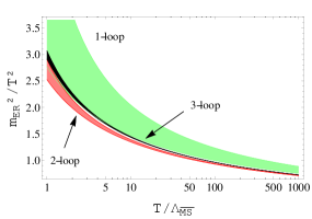
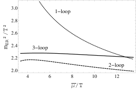
Figure 2: Left: dimensionless Debye mass $m_{\mathrm{ER}}^{2}/T^{2}$ as a function of the temperature $T$, in units of ${\Lambda_{\overline{\mbox{\tiny\rm{MS}}}}}$ and with the variation of $\bar{\mu}=(0.5...2.0)\times\bar{\mu}_{\text{opt}}$. Right: variation of the mass with respect to $\bar{\mu}$ at the scale $T/{\Lambda_{\overline{\mbox{\tiny\rm{MS}}}}}=2$ and with $\mu_{3}=\mu_{3,\text{opt}}$.

In Fig. 2, we analyze the running of the Debye mass with respect to the temperature ($T$). We have used the solution of the renormalization group equation of the 4d coupling $g$, in which the QCD $\beta$-function was truncated after ${\mathcal{O}}(g^{8})$. The parameter ${\Lambda_{\overline{\mbox{\tiny\rm{MS}}}}}$ corresponds to the QCD scale defined in Ref. Laine:2005ai , and here simply sets the scale through the $t$-dependence of the running coupling Eq. (21). The arbitrary scale $\bar{\mu}$ was chosen at the point where the effective coupling $g_{\mathrm{ER}}$ has a minimal sensitivity to it: $\bar{\mu}_{\text{opt}}/T\approx 2\pi$. The 3 bands in the plot arise by varying $\bar{\mu}=(0.5...2)\times\bar{\mu}_{\text{opt}}$. Using the prescription described above for choosing a sensible scale for the EQCD scale parameter, $\mu_{3}/T\approx 2.85$, we obtain a three-loop result with a vanishingly narrow band width.

From the figure, one notices a slight increase of the Debye mass with respect to the 2-loop result. In addition, the sensitivity with respect to the arbitrary scale $\bar{\mu}$ decreases, which indicates that the perturbative expansion up to 3-loop order shows good convergence properties.

4 A $g^{7}$ contribution to the QCD pressure

Having the 3-loop Debye mass at hand, we can use it to extract a gauge-invariant piece of a higher-order perturbative ($g^{7}$) correction to the QCD pressure. The order $g^{7}$ owes its importance to the fact that it represents, in the effective theory setup we are working in, the leading correction to what has been called the physical leading order, i.e. all terms up to order $g^{6}$ that, for the first time, include all potentially large logarithms entering the QCD pressure Kajantie:2002wa .

As already discussed in the introduction, in the effective theory framework, the QCD partition function factorizes, such that the pressure $p_{\mathrm{QCD}}$ splits into three parts $p_{\mathrm{E}},\,p_{\mathrm{M}}$ and $p_{\mathrm{G}}$ originating from contributions of the hard- $2\pi T$, soft- $gT$ and ultra-soft scale $g^{2}T$, respectively Braaten:1995jr ; Kajantie:2000iz . These three parts can be extracted as matching coefficients of QCD, EQCD and MQCD, along the following chain of equations (recall $d=3-2\epsilon$),

$$p_{\mathrm{QCD}}(T) =\lim_{V\rightarrow\infty}\frac{1}{V_{d+1}}\ln\int\!\!\mathcal{D}A_{\mu}^{a}\;\exp\Big{[}-\int_{0}^{1/T}\!\!\!\!\!\!\!{\rm d}\tau\int\!\!{\rm d}^{d}x\;\mathcal{L}^{\mathrm{4d}}_{\mathrm{QCD}}\Big{]}$$

$$=p_{\mathrm{E}}(T)+\lim_{V\rightarrow\infty}\frac{T}{V_{d}}\ln\int\!\!\mathcal{D}A_{k}^{a}\,\mathcal{D}A_{0}^{a}\;\exp\Big{[}-\int\!\!{\rm d}^{d}x\;\mathcal{L}^{\mathrm{3d}}_{\mathrm{EQCD}}\Big{]}$$

$$=p_{\mathrm{E}}(T)+p_{\mathrm{M}}(T)+\lim_{V\rightarrow\infty}\frac{T}{V_{d}}\ln\int\!\!\mathcal{D}A_{k}^{a}\;\exp\Big{[}-\int\!\!{\rm d}^{d}x\;\mathcal{L}^{\mathrm{3d}}_{\mathrm{MQCD}}\Big{]}$$

$$=p_{\mathrm{E}}(T)+p_{\mathrm{M}}(T)+p_{\mathrm{G}}(T)\,,$$ (23)

supplemented with the corresponding matching of the couplings, as has been explained in the previous chapters on the example of the chromo-electric screening mass.

It turns out that the different pieces in Eq. (23), when re-expressed in terms of the renormalized 4d gauge coupling $g_{\mathrm{R}}$ (and omitting logarithms of the coupling), contribute as

$$p_{\mathrm{E}} \sim T^{4}(1+g_{\mathrm{R}}^{2}+g_{\mathrm{R}}^{4}+g_{\mathrm{R}}^{6}+\dots)\;,$$ (24)

$$p_{\mathrm{M}} \sim T^{4}(g_{\mathrm{R}}^{3}+g_{\mathrm{R}}^{4}+g_{\mathrm{R}}^{5}+g_{\mathrm{R}}^{6}+g_{\mathrm{R}}^{7}+\dots)\;,$$ (25)

$$p_{\mathrm{G}} \sim T^{4}(g_{\mathrm{R}}^{6}+g_{\mathrm{R}}^{7}+\dots)\;.$$ (26)

Both parts of the pressure coming from the 3d reduced effective theories describing soft and ultra-soft effects, EQCD and MQCD, contain contributions of order $g_{\mathrm{R}}^{7}$. The latter part originates from matching of the MQCD gauge coupling $g_{\mathrm{M}}$, as $p_{\mathrm{G}}=Tg_{\mathrm{M}}^{6}c_{\mathrm{G}}$, with $c_{\mathrm{G}}$ being a non-perturbative coefficient determined in Kajantie:2002wa ; DiRenzo:2006nh , and the coupling $g_{\mathrm{M}}^{2}\sim g_{\mathrm{E}}^{2}(1+g_{\mathrm{E}}^{2}/m_{\mathrm{E}}+{\cal O}(g_{\mathrm{E}}^{4}/m_{\mathrm{E}}^{2}))\sim Tg_{\mathrm{R}}^{2}(1+g_{\mathrm{R}}+{\cal O}(g_{\mathrm{R}}^{2}))$ with coefficients known from e.g. Farakos:1994kx .

The contributions of order $g_{\mathrm{R}}^{7}$ to the pressure of hot QCD from the soft scale $gT$ entering through EQCD originate from a number of different sources. Within EQCD, the expansion reads (see e.g. Braaten:1995jr )

$$p_{\mathrm{M}}(T) =Tm_{\mathrm{ER}}^{3}\left[\frac{N^{2}\!-\!1}{12\pi}+a_{2}\,x+a_{2}^{\prime}\,y+a_{3}\,x^{2}+a_{3}^{\prime}\,x\,y+a_{4}\,x^{3}+a_{5}\,x^{4}+\dots\right]\,,$$ (27)

with known 2..4-loop coefficients $a_{2..4}$ Kajantie:2003ax , and $a_{5}$ coming from a 5-loop calculation of the EQCD pressure including contributions from higher-order operators Chapman:1994vk omitted in Eq. (2), both of which remain unknown to date. The expansion parameters above relate to the 4d coupling as

$$x\equiv\frac{g_{\mathrm{ER}}^{2}}{m_{\mathrm{ER}}}\sim g_{\mathrm{R}}(1+{\cal O}(g_{\mathrm{R}}^{2}))\quad,\quad y\equiv\frac{\lambda^{(1/2)}_{\mathrm{ER}}}{m_{\mathrm{ER}}}\sim g_{\mathrm{R}}^{3}(1+{\cal O}(g_{\mathrm{R}}^{2}))\;,$$ (28)

such that we can already fix the other $g^{7}$ pieces by multiplying out the expansion parameters and our new 3-loop result for $m_{\mathrm{E}}^{2}$. Writing

$$m_{\mathrm{ER}}^{2} =g_{\mathrm{R}}^{2}\,T^{2}\left[\alpha_{{\mathrm{E}}4}+\frac{g_{\mathrm{R}}^{2}}{(4\pi)^{2}}\,\alpha_{{\mathrm{E}}6}+\frac{g_{\mathrm{R}}^{4}}{(4\pi)^{4}}\,\alpha_{{\mathrm{E}}8}+\dots\right]\;,$$ (29)

where $\alpha_{{\mathrm{E}}8}$ represents our new 3-loop result of Eq. (3.2), this coefficient contributes a $g^{7}$ term to the QCD pressure, via

$$m_{\mathrm{ER}}^{3} =g_{\mathrm{R}}^{3}\,T^{3}\,\alpha_{{\mathrm{E}}4}^{3/2}\left[1+\frac{g_{\mathrm{R}}^{2}}{(4\pi)^{2}}\,\frac{3}{2}\,\frac{\alpha_{{\mathrm{E}}6}}{\alpha_{{\mathrm{E}}4}}+\frac{g_{\mathrm{R}}^{4}}{(4\pi)^{4}}\,\frac{3}{8}\,\frac{\alpha_{{\mathrm{E}}6}^{2}+4\alpha_{{\mathrm{E}}4}\alpha_{{\mathrm{E}}8}}{\alpha_{{\mathrm{E}}4}^{2}}+\dots\right]\;,$$ (30)

$$p_{\mathrm{M}}(T)|_{m_{\mathrm{ER}}^{3},g_{\mathrm{R}}^{7}} =T^{4}\frac{g_{\mathrm{R}}^{7}}{(4\pi)^{5}}\,\frac{N^{2}\!-\!1}{8}\,\frac{\alpha_{{\mathrm{E}}6}^{2}+4\alpha_{{\mathrm{E}}4}\alpha_{{\mathrm{E}}8}}{\alpha_{{\mathrm{E}}4}^{1/2}}$$

$$=8\pi^{2}T^{4}(N^{2}\!-\!1)\left[\frac{N}{3}\,\frac{g_{\mathrm{R}}^{2}}{(4\pi)^{2}}\right]^{\frac{7}{2}}\left[605L^{2}+479L-180L_{3}+\frac{1487}{4}-18\zeta(3)\right]\;,$$ (31)

with logarithms $L$ and $L_{3}$ as in Eq. (3.2) above.

5 Conclusions

In this paper, we have determined the Debye screening mass of hot Yang-Mills theory to 3-loop (NNLO) accuracy, by combining various results of a long-term project, with a number of independent ingredients, each of which needed novel state-of-the art techniques for a successful determination. While the feasibility of such a precision calculation in the thermal context was not at all clear from the outset, we have here succeeded to overcome the last major obstacle – namely to map a sum of seven non-trivial master sum-integrals (that remained after the IBP reduction algorithm had halted, but which would have been needed to an expansion depth for which no technique existed) to a small number of (three) computable cases. We have achieved this reduction in complexity of the calculation by a clever basis transformation, which was made possible by searching our extensive database of IBP relations.

To our utmost satisfaction, the final assembly of all building blocks revealed (a) gauge parameter independence, (b) a finite result after renormalization, and (c) good convergence properties. We were therefore able to add another term to the pool of known (and heavily used) matching coefficients of EQCD, and to utilize this fresh term right away, determining one of the physical next-to-leading order ($g^{7}$) contributions to the pressure of hot QCD. As we have discussed above, this is of course not the complete $g^{7}$ result, but represents a well-defined (and gauge invariant) contribution to it.

Thus, looking back on the many technical and systematic advances that have been made during this project, we conclude that a determination of the 3-loop effective gauge coupling $g_{\mathrm{E}}^{2}$, which originates from a (by one) higher moment of two-point functions and which is hence amenable to the same techniques as $m_{\mathrm{E}}^{2}$, should be within reach.

Another avenue for further investigations would be a generalization of our strategy to fermionic contributions, which we have ignored completely here, setting $N_{\mathrm{f}}=0$. While the reduction to basketball-type master integrals is done Moeller:2012da , open problems are finding a suitable basis change, and evaluating the corresponding fermionic masters – which, containing no zero-modes on fermionic lines, could however turn out to be less involved than the bosonic cases that we have used here.

The result for the Debye mass shows a good convergence in a large temperature range, suggesting that already at the three-loop order the corrections are numerically negligible, but would serve merely in future perturbative calculations (of observables such as the pressure of QCD) to ensure finite renormalized results (cancellation of UV divergences). In the light of the apparent fast convergence of the analytic result, a re-evaluation of the non-perturbative constant of the QCD screening mass can be considered Laine:1999hh ; Burnier:2015nsa since this latter quantity is in fact used in studies of quark gluon plasma parameters such as the jet quenching parameter Ghiglieri:2015zma ; Panero:2014sua .

Appendix A Lower-order ingredients

The one- and two-loop expressions entering Eq. (2.1) have been given in Ref. Moeller:2012da in terms of one-loop sum-integrals $I$. Their $N_{\mathrm{f}}=0$ pieces read

$$\Pi_{\mathrm{E}1} =N(d-1)^{2}\,I_{1}\;,$$ (32)

$$\Pi_{\mathrm{E}1}^{\prime} =-N\left[\frac{28-5d+d^{2}}{6}+(d-3)\xi\right]I_{2}\;,$$ (33)

$$\Pi_{\mathrm{E}1}^{\prime\prime} =N\left[\frac{46-7d+d^{2}}{30}+\frac{d-3}{3}\,\xi+\frac{d-6}{12}\,\xi^{2}\right]I_{3}\;,$$ (34)

$$\Pi_{\mathrm{E}2} =-N^{2}(1+\xi)(d-3)(d-1)^{2}\,I_{2}I_{1}\;,$$ (35)

$$\Pi_{\mathrm{E}2}^{\prime} =N^{2}\left[-\frac{72-42d+13d^{2}-d^{3}}{3d(d-7)}+\frac{d}{3}\,\xi+\frac{d-6}{6}\,\xi^{2}\right](d-1)^{2}\,I_{3}I_{1}+$$ (36)

$$+N^{2}\left[\frac{p(d)}{2d(d\!-\!7)(d\!-\!5)(d\!-\!2)}-\frac{44\!-\!29d\!+\!7d^{2}\!-\!d^{3}}{6(d-2)}\,\xi+\frac{16\!-\!13d\!+\!3d^{2}}{8(d-2)}\,\xi^{2}\right](d\!-\!3)\,I_{2}I_{2}\;,$$

with $p(d)=56+315d-231d^{2}+57d^{3}-5d^{4}$.

Appendix B Master sum-integrals

Let us define a generic notation for massless 3-loop vacuum sum-integrals

$$J_{abcdef}^{\alpha\beta\gamma}\equiv\begin{picture}(30.0,30.0)(0.0,10.0)\CArc(15,15)(15,0,360) \Line(15,0)(15,15)\Line(15,15)(25.5,25.5) \Line(15,15)(4.5,25.5)\Text(15,35)[]{\text{\scriptsize{$a$}}} \Text(0,3)[]{\text{\scriptsize{$b$}}}\Text(30,3)[]{\text{\scriptsize{$c$}}} \Text(7.5,15.5)[]{\text{\scriptsize{$d$}}}\Text(22.5,15.5)[]{\text{\scriptsize{$e$}}} \Text(18,6.5)[]{\text{\scriptsize{$f$}}}\end{picture}\equiv\hbox{$\sum$}\!\!\!\!\!\!\!\int_{PQR}\frac{(P_{0})^{\alpha}(Q_{0})^{\beta}(R_{0})^{\gamma}}{[P^{2}]^{a}[Q^{2}]^{b}[R^{2}]^{c}[(P-Q)^{2}]^{d}[(P-R)^{2}]^{e}[(Q-R)^{2}]^{f}}\;,$$ (37)

where all momenta are understood bosonic. Let us remark that from the outset, only integrals $J^{000}_{abcdef}$ enter the calculation; however, due to the fact that the IBP relations act in the $d$ spatial dimensions only and hence explicitly break $(d\!+\!1)$-dimensional rotational invariance introducing the 4-vector $U=(1,{\mathbf{0}})$, the numerator structure of Eq. (37) occurs naturally in the reduction step. The original integral reduction Eq. (6) contains only basketball-type sum-integrals $J_{ab00ef}^{\alpha\beta\gamma}$ as well as trivial products of one-loop cases

$$J_{abc000}^{\alpha\beta\gamma} =I_{a}^{\alpha}\,I^{\beta}_{b}\,I^{\gamma}_{c}\;,$$ (38)

$$I_{s}^{a} \equiv\hbox{$\sum$}\!\!\!\!\!\!\!\int_{Q}\frac{|Q_{0}|^{a}}{[Q^{2}]^{s}}=\frac{2T\,\zeta(2s-a-d)}{(2\pi T)^{2s-a-d}}\,\frac{\Gamma(s-\frac{d}{2})}{(4\pi)^{d/2}\Gamma(s)}\;,\quad I_{s}\equiv\hbox{$\sum$}\!\!\!\!\!\!\!\int_{Q}\frac{1}{[Q^{2}]^{s}}=I_{s}^{0}\;.$$ (39)

Of these, we need the products

$$I_{3}I_{1}I_{1} =\frac{T^{2}}{(4\pi)^{4}}\left(\frac{e^{\gamma}}{4\pi T^{2}}\right)^{3\epsilon}\frac{2\,\zeta(3)}{144}\bigg{[}1+2\epsilon(3-3{\gamma_{\small\rm E}}+Z_{3}+2Z_{1})+{\mathcal{O}}(\epsilon^{2})\bigg{]}\;,$$ (40)

$$I_{2}I_{2}I_{1} =\frac{T^{2}}{(4\pi)^{4}}\left(\frac{e^{\gamma}}{4\pi T^{2}}\right)^{3\epsilon}\frac{1}{12\,\epsilon^{2}}\bigg{[}1+2\epsilon(1-{\gamma_{\small\rm E}}+Z_{1})+2\epsilon^{2}(2+\tfrac{3\pi^{2}}{8}+2Z_{1}-$$

$$-{\gamma_{\small\rm E}}({\gamma_{\small\rm E}}+2+2Z_{1})-4\gamma_{1}+\tfrac{\zeta^{\prime\prime}(-1)}{\zeta(-1)})+{\mathcal{O}}(\epsilon^{3})\bigg{]}\;,$$ (41)

containing the numbers ${\gamma_{\small\rm E}}$ and $\gamma_{1}$ arising from the expansion of the Riemann Zeta function around its pole at unity, $\zeta(1-\epsilon)\approx-1/\epsilon+{\gamma_{\small\rm E}}+\gamma_{1}\epsilon+\dots$, as well as $Z_{n}\equiv\zeta^{\prime}(-n)/\zeta(-n)$. The specific cases on the left-hand sides of Eqs. (47)-(D) are more complicated integrals, which have however already been evaluated up to their constant terms in a number of tour de force computations documented in Refs. Andersen:2008bz ; Schroder:2012hm , Ghisoiu:2012kn and Ghisoiu:2012yk , respectively, from where we collect the results for convenience:

$$J_{11} \equiv J_{111110}^{000} \;=\; \frac{T^{2}}{(4\pi)^{4}}\left(\frac{1}{4\pi T^{2}}\right)^{3\epsilon}\frac{-1}{4\,\epsilon^{2}}\left[1+\!\left(\frac{4}{3}\!+\!{\gamma_{\small\rm E}}\!+\!2Z_{1}\right)\epsilon+\!c_{1}\epsilon^{2}+\!{\mathcal{O}}(\epsilon^{3})\right]\;,$$ (42)

$$J_{12} \equiv J_{211110}^{020} \;=\; \frac{T^{2}}{(4\pi)^{4}}\left(\frac{1}{4\pi T^{2}}\right)^{3\epsilon}\frac{1}{96\,\epsilon^{2}}\left[1+\!\left(\frac{67}{6}\!+\!{\gamma_{\small\rm E}}\!+\!2Z_{1}\right)\epsilon+\!c_{2}\epsilon^{2}+\!{\mathcal{O}}(\epsilon^{3})\right]\;,$$ (43)

$$J_{13} \equiv J_{31111-2}^{000} \;=\; \frac{T^{2}}{(4\pi)^{4}}\left(\frac{1}{4\pi T^{2}}\right)^{3\epsilon}\frac{-5}{36\,\epsilon^{2}}\left[1+\!\left(\frac{71}{30}\!+\!{\gamma_{\small\rm E}}\!+\!2Z_{1}\right)\epsilon+\!c_{3}\,\epsilon^{2}+\!{\mathcal{O}}(\epsilon^{3})\right]\;.$$ (44)

The constant parts are known numerically only, and have been determined in the above-mentioned references to be $c_{1}\approx+43.8676(1)$, $c_{2}\approx+93.0894417(2)$ and $c_{3}\approx+44.629857(1)$. In the present computation, however, these constant parts do not contribute, since the integrals are multiplied by pre-factors $\sim\epsilon$, cf. Eq. (3.1).

Appendix C Coefficients of Eq. (6)

The coefficients $\alpha_{1...10}$ of Eq. (6), as determined in Ref. Moeller:2012da , are rational functions in $d$ (recall that we use $d=3-2\epsilon$ in this work), in some cases also containing the gauge parameter $\xi$,

$$\alpha_{1} =-\frac{(d-1)a_{1}(d)}{24(d-6)(d-5)(d-4)(d-3)(d-2)(3d-17)}\;,$$

$$\alpha_{2} =-\frac{3(d-1)a_{2}(d)}{4(d-6)(d-5)(d-3)(d-2)(3d-17)}\;,$$

$$\alpha_{3} =-\frac{(d-1)a_{3}(d)}{4(d-6)(d-5)(d-2)(3d-17)}\;,$$

$$\alpha_{4} =-\frac{(d-1)a_{4}(d)}{12(d-6)(d-5)(d-3)(d-2)(3d-17)}\;,$$

$$\alpha_{5} =\frac{36(d-11)(d-9)(d-1)}{(d-6)(d-2)(3d-17)}\;,$$

$$\alpha_{6} =\frac{512(d-1)(1954-641d+48d^{2})}{(d-5)(d-3)(d-2)}\;,$$

$$\alpha_{7} =-\frac{49152(d-1)}{(d-5)(d-3)(d-2)}\;,$$

$$\alpha_{8} =-\frac{122880(d-1)}{(d-5)(d-3)(d-2)}\;,$$

$$\alpha_{9} =-\frac{(d-1)a_{9}(d)}{4(d-6)(d-5)(d-3)(d-2)(3d-17)}+(d-1)^{4}\xi+\frac{(d-6)(d-1)^{4}}{12}\,\xi^{2}\;,$$

$$\alpha_{10} =-\frac{(d-1)a_{10}(d)}{4(d-7)(d-6)(d-5)^{2}(d-3)(d-2)(3d-17)}$$

$$+\frac{(d-3)(d-1)^{2}(16-13d+2d^{2})}{2(d-2)}\,\xi+\frac{(d-3)(d-1)^{2}(16-13d+3d^{2})}{8(d-2)}\,\xi^{2}\;,$$ (45)

where we have for convenience used the abbreviations

$$a_{1}(d) =5982874650-9764062527d+6860483170d^{2}-2710270726d^{3}+658312418d^{4}$$

$$-100632587d^{5}+9447810d^{6}-497520d^{7}+11232d^{8},$$

$$a_{2}(d) =14947857-14330519d+5758990d^{2}-1245506d^{3}+153345d^{4}-10215d^{5}+288d^{6},$$

$$a_{3}(d) =8970183-7006766d+2180196d^{2}-337402d^{3}+25941d^{4}-792d^{5},$$

$$a_{4}(d) =1784823003-1809632517d+757032878d^{2}-167080938d^{3}+20490319d^{4}$$

$$-1321425d^{5}+34920d^{6},$$

$$a_{9}(d) =17888670-22432867d+10547330d^{2}-2313976d^{3}+186752d^{4}+17787d^{5}$$

$$-5140d^{6}+416d^{7}-12d^{8},$$

$$a_{10}(d) =-835002999+1120616178d-653300169d^{2}+218578438d^{3}-47171745d^{4}$$

$$+7193512d^{5}-870355d^{6}+92054d^{7}-8000d^{8}+458d^{9}-12d^{10}.$$ (46)

Appendix D IBP relations for basis transformation

The idea of performing a basis transformation on $\Pi_{\mathrm{E}3}$ translates into going some steps back into its IBP reduction Moeller:2012da . The goal is to search for relations that change the coefficients of the master sum-integrals (cf. the last paragraph of App. C in Moeller:2012da ) in such a way as to eliminate all factors of $(d-3)$ in the denominator. While it is not at all clear from the outset that this can always be achieved, it happens indeed if we use the following three automatically generated IBP relations, expressed in terms of the basis of basketball-type 3-loop master integrals defined in Eq. (7):

$$J_{11} =\frac{2(47-24d+3d^{2})}{3(d-3)^{2}(d-4)}\,J_{1}+\frac{16}{3(d-3)^{2}}\,J_{4}\;,$$ (47)

$$J_{12} =\frac{(d-9)(d-7)(d-2)}{2(d-6)(d-5)(d-4)(d-3)^{2}}\,I_{3}I_{1}I_{1}+\frac{519-312d+61d^{2}-4d^{3}}{2(d-6)(d-5)^{2}(d-4)(d-3)}\,I_{2}I_{2}I_{1}-$$

$$-\frac{(3d-10)(10791-9060d+2806d^{2}-380d^{3}+19d^{4})}{12(d-6)(d-5)(d-4)^{2}(d-3)^{2}}\,J_{1}+$$

$$+\frac{3(d-7)}{2(d-6)(d-4)(d-3)}\,J_{2}-\frac{(d-9)(d-7)}{2(d-6)(d-5)(d-4)(d-3)}\,J_{3}+$$

$$+\frac{31401-16707d+2951d^{2}-173d^{3}}{6(d-6)(d-5)(d-4)(d-3)^{2}}\,J_{4}+\frac{512}{(d-5)(d-4)(d-3)^{2}}\,J_{6}\;,$$ (48)

$$J_{13} =\frac{b_{1}(d)\,J_{1}+18(d-4)b_{2}(d)\,J_{2}+6(d-4)(d-3)b_{3}(d)\,J_{3}+2(d-4)b_{4}(d)\,J_{4}}{12(d-7)(d-6)(d-5)(d-4)(d-3)^{2}(d-2)(d-1)(3d-17)}-$$

$$-\frac{72(d-11)(d-9)\,J_{5}}{(d-7)(d-6)(d-3)(d-2)(d-1)(3d-17)}+$$

$$+1024\,\frac{(-1970+665d-56d^{2})\,J_{6}+96\,J_{7}+240\,J_{8}}{(d-7)(d-5)(d-3)^{2}(d-2)(d-1)}+$$

$$+\frac{(d-7)(d-5)b_{9}(d)\,I_{3}I_{1}I_{1}+b_{10}(d)\,I_{2}I_{2}I_{1}}{2(d-7)^{2}(d-6)(d-5)^{2}(d-3)^{2}(d-2)(d-1)(3d-17)}\;,$$ (49)

where Eq. (D) contains the polynomials

$$b_{1}(d) =6039084810-9921665183d+7037865926d^{2}-2817068438d^{3}+696438686d^{4}$$

$$-108972587d^{5}+10546622d^{6}-577632d^{7}+13716d^{8}\;,$$

$$b_{2}(d) =14890737-14196135d+5642398d^{2}-1196706d^{3}+142785d^{4}-9079d^{5}+240d^{6}\;,$$

$$b_{3}(d) =8935911-6940606d+2138852d^{2}-326810d^{3}+24757d^{4}-744d^{5}\;,$$

$$b_{4}(d) =1801692987-1846811125d+786404686d^{2}-178072266d^{3}+22616879d^{4}$$

$$-1527809d^{5}+42888d^{6}\;,$$

$$b_{9}(d) =18419886-24034307d+12505438d^{2}-3593336d^{3}+677116d^{4}-95461d^{5}$$

$$+10336d^{6}-736d^{7}+24d^{8}\;,$$

$$b_{10}(d) =-834536043+1116882072d-645264933d^{2}+210429806d^{3}-42367633d^{4}$$

$$+5387676d^{5}-421763d^{6}+18526d^{7}-348d^{8}\;.$$ (50)

References

• (1) N. P. Landsman and C. G. van Weert, Real and Imaginary Time Field Theory at Finite Temperature and Density, Phys. Rept.  145 (1987) 141.
• (2) A. D. Linde, Infrared Problem in Thermodynamics of the Yang-Mills Gas, Phys. Lett. B 96 (1980) 289.
• (3) K. Kajantie and J. I. Kapusta, Infrared Limit Of The Axial Gauge Gluon Propagator At High Temperature, Phys. Lett. B 110 (1982) 299.
• (4) K. Kajantie and J. I. Kapusta, Behavior of Gluons at High Temperature, Annals Phys.  160 (1985) 477.
• (5) T. Furusawa and K. Kikkawa, Gauge Invariant Values Of Gluon Masses At High Temperature, Phys. Lett. B 128 (1983) 218.
• (6) T. Toimela, On The Magnetic And Electric Masses Of The Gluons In The General Covariant Gauge, Z. Phys. C 27 (1985) 289 [Erratum-ibid. C 28 (1985) 162].
• (7) P. B. Arnold and L. G. Yaffe, The NonAbelian Debye screening length beyond leading order, Phys. Rev. D 52 (1995) 7208 [hep-ph/9508280].
• (8) D. Bieletzki, K. Lessmeier, O. Philipsen and Y. Schröder, Resummation scheme for 3d Yang-Mills and the two-loop magnetic mass for hot gauge theories, JHEP 1205 (2012) 058 [arXiv:1203.6538].
• (9) R. Kobes, G. Kunstatter and A. Rebhan, QCD plasma parameters and the gauge dependent gluon propagator, Phys. Rev. Lett.  64, 2992 (1990).
• (10) R. Kobes, G. Kunstatter and A. Rebhan, Gauge dependence identities and their application at finite temperature, Nucl. Phys. B 355 (1991) 1.
• (11) A. K. Rebhan, The NonAbelian Debye mass at next-to-leading order, Phys. Rev. D 48 (1993) 3967 [hep-ph/9308232].
• (12) E. Braaten and A. Nieto, Next-to-leading order Debye mass for the quark - gluon plasma, Phys. Rev. Lett.  73 (1994) 2402 [hep-ph/9408273].
• (13) A. Hart, M. Laine and O. Philipsen, Static correlation lengths in QCD at high temperatures and finite densities, Nucl. Phys. B 586 (2000) 443 [hep-ph/0004060].
• (14) M. Laine and M. Vepsäläinen, On the smallest screening masses in hot QCD, JHEP 0909 (2009) 023 [arXiv:0906.4450].
• (15) J. Möller and Y. Schröder, Three-loop matching coefficients for hot QCD: Reduction and gauge independence, JHEP 1208 (2012) 025 [arXiv:1207.1309].
• (16) P. H. Ginsparg, First Order and Second Order Phase Transitions in Gauge Theories at Finite Temperature, Nucl. Phys. B 170 (1980) 388.
• (17) T. Appelquist and R. D. Pisarski, High-Temperature Yang-Mills Theories and Three-Dimensional Quantum Chromodynamics, Phys. Rev. D 23 (1981) 2305.
• (18) K. Kajantie, M. Laine, K. Rummukainen and M. E. Shaposhnikov, Generic rules for high temperature dimensional reduction and their application to the standard model, Nucl. Phys. B 458 (1996) 90 [hep-ph/9508379].
• (19) A. Hietanen, K. Kajantie, M. Laine, K. Rummukainen and Y. Schröder, Plaquette expectation value and gluon condensate in three dimensions, JHEP 0501 (2005) 013 [hep-lat/0412008].
• (20) A. Hietanen and A. Kurkela, Plaquette expectation value and lattice free energy of three-dimensional SU(N) gauge theory, JHEP 0611 (2006) 060 [hep-lat/0609015].
• (21) S. Chapman, A New dimensionally reduced effective action for QCD at high temperature, Phys. Rev. D 50 (1994) 5308 [hep-ph/9407313].
• (22) J. Möller and Y. Schröder, Dimensionally reduced QCD at high temperature, Prog. Part. Nucl. Phys.  67 (2012) 168.
• (23) L. F. Abbott, The Background Field Method Beyond One Loop, Nucl. Phys. B 185 (1981) 189.
• (24) L. F. Abbott, Introduction to the Background Field Method, Acta Phys. Polon. B 13 (1982) 33.
• (25) E. Braaten and A. Nieto, Free energy of QCD at high temperature, Phys. Rev. D 53 (1996) 3421 [hep-ph/9510408].
• (26) P. Nogueira, Automatic Feynman graph generation, J. Comput. Phys.  105 (1993) 279.
• (27) P. Nogueira, Abusing qgraf, Nucl. Instrum. Meth. A 559 (2006) 220.
• (28) J. A. M. Vermaseren, New features of FORM, math-ph/0010025.
• (29) J. Kuipers, T. Ueda, J. A. M. Vermaseren and J. Vollinga, FORM version 4.0, Comput. Phys. Commun.  184 (2013) 1453 [arXiv:1203.6543].
• (30) S. Laporta, High precision calculation of multiloop Feynman integrals by difference equations, Int. J. Mod. Phys. A 15 (2000) 5087 [hep-ph/0102033].
• (31) M. Nishimura and Y. Schröder, IBP methods at finite temperature, JHEP 1209 (2012) 051 [arXiv:1207.4042].
• (32) http://www.physik.uni-bielefeld.de/theory/e6/BI-TP-2012-25.html
• (33) A. Gynther, M. Laine, Y. Schröder, C. Torrero and A. Vuorinen, Four-loop pressure of massless O(N) scalar field theory, JHEP 0704 (2007) 094 [hep-ph/0703307].
• (34) J. Möller and Y. Schröder, Open problems in hot QCD, Nucl. Phys. Proc. Suppl.  205-206 (2010) 218 [arXiv:1007.1223].
• (35) P. B. Arnold and C. X. Zhai, The Three loop free energy for pure gauge QCD, Phys. Rev. D 50 (1994) 7603 [hep-ph/9408276].
• (36) P. B. Arnold and C. X. Zhai, The Three loop free energy for high temperature QED and QCD with fermions, Phys. Rev. D 51 (1995) 1906 [hep-ph/9410360].
• (37) K. G. Chetyrkin, M. Faisst, C. Sturm and M. Tentyukov, epsilon-finite basis of master integrals for the integration-by-parts method, Nucl. Phys. B 742 (2006) 208 [hep-ph/0601165].
• (38) O. V. Tarasov, Connection between Feynman integrals having different values of the space-time dimension, Phys. Rev. D 54 (1996) 6479 [hep-th/9606018].
• (39) I. Ghişoiu and Y. Schröder, A new three-loop sum-integral of mass dimension two, JHEP 1209 (2012) 016 [arXiv:1207.6214].
• (40) I. Ghişoiu and Y. Schröder, A New Method for Taming Tensor Sum-Integrals, JHEP 1211 (2012) 010 [arXiv:1208.0284].
• (41) A. Rajantie, SU(5) + adjoint Higgs model at finite temperature, Nucl. Phys. B 501 (1997) 521 [hep-ph/9702255].
• (42) M. Laine and A. Rajantie, Lattice continuum relations for 3-D SU(N) + Higgs theories, Nucl. Phys. B 513 (1998) 471 [hep-lat/9705003].
• (43) K. Farakos, K. Kajantie, K. Rummukainen and M. E. Shaposhnikov, 3-D physics and the electroweak phase transition: Perturbation theory, Nucl. Phys. B 425 (1994) 67 [hep-ph/9404201].
• (44) N. P. Landsman, Limitations to Dimensional Reduction at High Temperature, Nucl. Phys. B 322 (1989) 498.
• (45) M. Laine and Y. Schröder, Two-loop QCD gauge coupling at high temperatures, JHEP 0503 (2005) 067 [hep-ph/0503061].
• (46) K. A. Olive et al. [Particle Data Group Collaboration], Review of Particle Physics, Chin. Phys. C 38 (2014) 090001.
• (47) K. G. Chetyrkin, B. A. Kniehl and M. Steinhauser, Strong coupling constant with flavor thresholds at four loops in the MS scheme, Phys. Rev. Lett.  79 (1997) 2184 [hep-ph/9706430].
• (48) W. A. Bardeen, A. J. Buras, D. W. Duke and T. Muta, Deep Inelastic Scattering Beyond the Leading Order in Asymptotically Free Gauge Theories, Phys. Rev. D 18 (1978) 3998.
• (49) K. Kajantie, M. Laine, K. Rummukainen and Y. Schröder, The Pressure of hot QCD up to g6 ln(1/g), Phys. Rev. D 67 (2003) 105008 [hep-ph/0211321].
• (50) K. Kajantie, M. Laine, K. Rummukainen and Y. Schröder, How to resum long distance contributions to the QCD pressure?, Phys. Rev. Lett.  86 (2001) 10 [hep-ph/0007109].
• (51) F. Di Renzo, M. Laine, V. Miccio, Y. Schröder and C. Torrero, The Leading non-perturbative coefficient in the weak-coupling expansion of hot QCD pressure, JHEP 0607 (2006) 026 [hep-ph/0605042].
• (52) K. Kajantie, M. Laine, K. Rummukainen and Y. Schröder, Four loop vacuum energy density of the SU(N(c)) + adjoint Higgs theory, JHEP 0304 (2003) 036 [hep-ph/0304048].
• (53) M. Laine and O. Philipsen, The Nonperturbative QCD Debye mass from a Wilson line operator, Phys. Lett. B 459 (1999) 259 [hep-lat/9905004].
• (54) Y. Burnier and A. Rothkopf, A gauge invariant Debye mass and the complex heavy-quark potential, arXiv:1506.08684.
• (55) J. Ghiglieri and D. Teaney, Parton energy loss and momentum broadening at NLO in high temperature QCD plasmas, arXiv:1502.03730.
• (56) M. Panero, K. Rummukainen and A. Schäfer, Jet quenching from the lattice, Nucl. Phys. A 931 (2014) 393 [arXiv:1407.2963].
• (57) J. A. M. Vermaseren, Axodraw, Comput. Phys. Commun.  83 (1994) 45.
• (58) J. O. Andersen and L. Kyllingstad, Four-loop Screened Perturbation Theory, Phys. Rev. D 78 (2008) 076008 [arXiv:0805.4478].
• (59) Y. Schröder, A fresh look on three-loop sum-integrals, JHEP 1208 (2012) 095 [arXiv:1207.5666].