Early-time cosmological solutions in scalar-Gauss-Bonnet theory

Abstract

We consider a gravitational theory that contains the Einstein term, a scalar field and the quadratic Gauss-Bonnet term. We focus on the early-universe dynamics, and demonstrate that the Ricci scalar does not affect the cosmological solutions at early times, when the curvature is strong. We then consider a pure scalar-GB theory with a quadratic coupling function: for a negative coupling parameter, we obtain solutions that contain always an inflationary, de Sitter phase, while for a positive coupling function, we find instead expanding singularity-free solutions.

1 Introduction

The generalised gravitational theories that contain, apart from the Einstein-Hilbert term, additional gravitational terms or extra fields, have been intensively studied over the last decades during the quest for the ultimate gravitational theory that would be valid both at large and small energy scales. These theories contain, among others, the heterotic superstring effective theory [1, 2, 3] or the Lovelock theory [4]. The quadratic Gauss-Bonnet term is present in both of the aforementioned theories and its implications for gravity and cosmology have been extensively studied [5, 6, 7, 8, 9, 10, 11, 12, 13, 14].

Being a topological invariant in four dimensions, the Gauss-Bonnet (GB) term must be coupled to a field, usually a scalar field, to remain in the theory. Therefore, in this work we consider a 4-dimensional theory that contains the Ricci scalar, the GB term and a non-minimally coupled scalar field. We will focus on the dynamics of the early universe, and argue that during that era the presence of the Ricci scalar adds nothing to the dynamics of the cosmological solution. For the case of a quadratic coupling function between the scalar field and the GB term, we demonstrate that this coupled system leads to cosmological solutions with interesting characteristics that are classified by the sign of the coupling function constant.

2 The Theoretical Framework

We will focus on a generalised gravitational theory that contains the usual Einstein term – i.e. the Ricci scalar $R$, a scalar field $\phi$ and the higher-derivative Gauss-Bonnet term $R^{2}_{\rm GB}$. The action functional of this string-inspired theory reads

$${\cal S}=\int d^{4}x\,\sqrt{-g}\left[\frac{R}{2}-\frac{(\nabla\phi)^{2}}{2}+\frac{1}{8}\,f(\phi)R^{2}_{\rm GB}\right].$$ (1)

The scalar field is coupled non-minimally to gravity via a general coupling function $f(\phi)$ to the quadratic Gauss-Bonnet term, that is defined as

$$R^{2}_{\rm GB}=R_{\mu\nu\rho\sigma}R^{\mu\nu\rho\sigma}-4R_{\mu\nu}R^{\mu\nu}+R^{2}\,.$$ (2)

We will also assume that the aforementioned scalar field is the dominant agent at the early universe and all other forms of matter/energy can be ignored during that time.

If we vary the action (1) with respect to the scalar field $\phi$ and the metric tensor $g_{\mu\nu}$, we obtain the scalar and gravitational field equations, respectively. Assuming that the line-element is described by the Friedmann-Lemaître-Robertson-Walker form

$$ds^{2}=-dt^{2}+a^{2}(t)\left[\frac{dr^{2}}{1-kr^{2}}+r^{2}\,(d\theta^{2}+\sin^{2}\theta\,d\varphi^{2})\right],$$ (3)

with a scale factor $a(t)$ and spatial curvature $k=0,\pm 1$, the field equations take the explicit form

$$\ddot{\phi}+3H\dot{\phi}-3f^{\prime}\bigl{(}H^{2}+\frac{k}{a^{2}}\bigr{)}(H^{2}+\dot{H}) =0\,,$$ (4)

$$3(1+H\dot{f})\bigl{(}H^{2}+\frac{k}{a^{2}}\bigr{)} =\frac{\dot{\phi}^{2}}{2}\,,$$ (5)

$$2(1+H\dot{f})(H^{2}+\dot{H})+(1+\ddot{f})\bigl{(}H^{2}+\frac{k}{a^{2}}\bigr{)} =-\frac{\dot{\phi}^{2}}{2}\,.$$ (6)

In the above, we have used the expression of the Gauss-Bonnet term for the line-element (3), that is

$$R^{2}_{GB}=24\,\bigl{(}H^{2}+\frac{k}{a^{2}}\bigr{)}(H^{2}+\dot{H})\,,$$ (7)

where $H\equiv\dot{a}/a$ is the Hubble parameter and the dot denotes derivative with respect to time.

One cannot help noticing that, for a constant coupling function $f(\phi)$, the GB term being a topological invariant completely disappears from the field equations. On the other hand, when present in the theory, it provides a non-trivial potential for the scalar field that is otherwise forced to adopt a constant configuration. A question that readily arises is whether the presence, or absence, of the Ricci scalar really modifies the dynamics of the ensuing cosmological solutions at very early times. We address this question in the following section.

3 The Complete Theory with a Linear Coupling

In this section, we will assume that the function $f(\phi)$ is a linear function of the field $\phi$, i.e. $f(\phi)=\lambda\phi$, where $\lambda$ is a coupling constant. Then, the scalar equation (4) can be easily integrated once with respect to time to yield the relation

$$\dot{\phi}=\frac{C}{a^{3}}+\frac{\lambda\dot{a}\,(3k+\dot{a}^{2})}{a^{3}}\,,$$ (8)

with $C$ an integration constant. Clearly, the effect of the GB term to the scalar-field dynamics is encoded in the second term of the above expression, that is proportional to $\lambda$. Henceforth, we will focus on this term and thus we set, for simplicity, $C=0$.

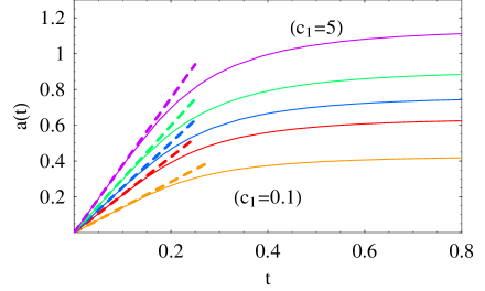
Figure 1: The scale factor $a(t)$ in terms of time, for a linear coupling function and $\lambda=0.1$, and for the values $c_{1}=0.1,0.5,1,2,5$ (from bottom to top).

If we rearrange Eqs. (4)-(6), and use Eq. (8) to replace any remaining $\dot{\phi}$’s (for further details on this, see [KGD-long]), we arrive at the constraint equation

$$3(k+\dot{a}^{2})^{2}\left[4+\lambda^{2}\,\frac{3\ddot{a}}{a^{3}}\,(k+\dot{a}^{2})\right]+\lambda^{2}\,\frac{\ddot{a}{\dot{a}}^{2}}{a^{3}}\,(3k+\dot{a}^{2})^{2}=0.$$ (9)

The above equation can be explicitly integrated twice only for $k=0$, in which case it leads to the solution

$$a(t)\,F\left[\frac{1}{4},\frac{1}{4},\frac{5}{4};\frac{3a^{4}(t)}{c_{1}}\right]=\left(\frac{2c_{1}}{5\lambda^{2}}\right)^{1/4}(t+t_{0})\,.$$ (10)

In the above, $F(a,b,c;x)$ stands for the hypergeometric function and $c_{1}$ is a constant. The general behaviour of $a(t)$ is depicted in Fig. 1. In the limit $a\rightarrow 0$, the above reduces to a linear relation between the scale factor and the time coordinate.

We will now focus on the early-time limit from the beginning and ignore the presence of the Ricci scalar. Then, a similar rearrangement of the field equations leads directly to the constraint $\ddot{a}=0$ and to the linear solution $a(t)=At+B$ – these solutions are also shown in Fig. 1. Therefore, as expected, in the strong-curvature regime and when the quadratic GB term is present, the linear term adds nothing to the dynamics of the cosmological solution and thus it may be altogether ignored. The same conclusion follows by considering the solution for the scalar field.

4 The Scalar-GB Theory with a Quadratic Coupling

Unfortunately, a similar analysis for the case of a quadratic coupling function cannot be performed due to the complexity of the corresponding field equations. However, as the coupling function $f(\phi)$ determines the weight of the GB term in the theory, we expect that its explicit form merely determines the point in time where the GB term begins to dominate over the linear Ricci term. Thus, choosing appropriately the time regime, we can always consider a pure scalar-GB theory and its dynamics at the early universe.

Therefore, focusing on the case of a quadratic coupling function, i.e. $f(\phi)=\lambda\phi^{2}$, and repeating the previous analysis, we arrive now at the constraint [15, 16]

$$(k+5{\dot{a}}^{2})\,\ddot{a}\,a^{3}+24\lambda\,{\dot{a}}^{2}\,(k+{\dot{a}}^{2})^{2}=0\,.$$ (11)

The above equation does not contain $\phi(t)$, and, for the case again of a flat universe ($k=0$), it can be integrated once to give

$$\frac{5}{2{\dot{a}}^{2}}=C_{1}-\frac{12\lambda}{a^{2}}\,.$$ (12)

Depending on the values of the integration constant $C_{1}$ and the Gauss-Bonnet coupling parameter $\lambda$, we may obtain a variety of cosmological solutions with interesting characteristics. Here, we present a sample of them classified by the sign of $\lambda$.

4.1 The case with $\lambda<0$

If the coupling constant $\lambda$ is negative, then the integration constant $C_{1}$ can have every possible value. Starting with the case of $C_{1}=0$, a simple integration of Eq. (12) yields the solution [15, 16]:

$$a(t)=a_{0}\,\exp\biggl{(}\pm\sqrt{\frac{5}{24|\lambda|}}\,t\biggr{)}.$$ (13)

If we choose the positive sign, the above solution describes an inflationary, de Sitter-type cosmological solution. The scalar field, whose expression may easily be found through Eq. (5), is also given by a similar exponential, but decaying, expression. Both quantities evolve faster with time the smaller the coupling constant $\lambda$ is. This so-called GB inflation [15] is supported only by the GB coupling of the scalar field and needs no additional potential with particular features as in the more traditional models [17, 18, 19]. The necessary number of e-foldings can also follow without introducing trans-planckian field values [15].

A more interesting family of solutions arises in the case where $C_{1}$ is positive. In that case, Eq. (12) upon integration leads to the relation

$$\sqrt{a^{2}+\nu^{2}}+\nu\ln\left(\frac{\sqrt{a^{2}+\nu^{2}}-\nu}{a}\right)=\pm\sqrt{\frac{5}{2C_{1}}}\,(t+t_{0})\,,$$ (14)

where $\nu^{2}\equiv 12|\lambda|/C_{1}$. The behaviour of $a(t)$ in terms of time, for the solution with the (+)-sign, is depicted in Fig. 2(a): the scale factor is expanding with time, with a faster pace at early times and a smaller one later. Indeed, in the limit $a\rightarrow 0$, we recover the pure de Sitter solution (13) found above, while for $a^{2}\gg\nu^{2}$, we obtain a Milne-type linearly expanding solution. Thus, these solutions accommodate an early inflationary phase with a natural exit mechanism at later times. The scalar field can be expressed in terms of the scale factor and is found to follow a decreasing pattern between two constant values [15, 16].

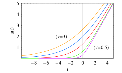
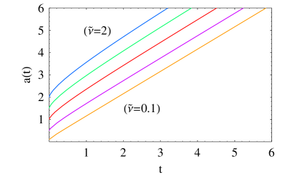
Figure 2: The scale factor $a(t)$ versus time for the cosmological solutions with: (a) $\lambda<0$, $C_{1}>0$ and $\nu=0.5,1,1.5,2,3$, and (b) with $\lambda>0$, $C_{1}>0$ and $\tilde{\nu}=0.1,0.5,1,1.5,2$.

4.2 The case with $\lambda>0$

If the coupling parameter $\lambda$ is positive, then $C_{1}$ is allowed to take only positive values, too. This time, Eq. (12) leads, upon integration again, to the relation [16]

$$\sqrt{a^{2}-\tilde{\nu}^{2}}-\tilde{\nu}\arccos\left(\frac{\tilde{\nu}}{a}\right)=\pm\sqrt{\frac{5}{2C_{1}}}\,(t+t_{0})\,.$$ (15)

where now $\tilde{\nu}^{2}\equiv 12\lambda/C_{1}$. The mathematical consistence of the above relation demands that $a^{2}\geq\tilde{\nu}^{2}$. As a result, $\tilde{\nu}$ is the smallest allowed value of the scale factor in this model, and the corresponding solutions are thus singularity-free. The profile of the solution, for the (+)-sign, is depicted in Fig. 2(b). For large values of the scale factor, the expansion becomes linear; for small values of $a(t)$ though, we find the asymptotic solution [16]

$$a(t)\simeq\tilde{\nu}\,[1+(At+B)^{2/3}]\,,$$ (16)

which reveals its regular behaviour for any finite values of the time-coordinate and the role of $\tilde{\nu}$ as the lower bound of the scale factor of the universe. The scalar field for this class of solutions starts from a zero value and increases towards an asymptotic constant value.

A similar analysis for a general coupling function $f(\phi)=\lambda\phi^{n}$, where $n$ is an integer number, reveals [16] that expanding, singularity-free solutions arise only for the case of $n=2$ studied above. We consider this not to be a coincidence since the quadratic coupling function falls into a general class of functions that have similar characteristics with the heterotic string effective coupling function [6]– singularity-free solutions were numerically shown to exist in the context of the latter theory [5] as well as in the theory with a quadratic coupling function [6], and here we have demonstrated their existence analytically even in the absence of the Ricci scalar.

5 Conclusions

In the context of the Einstein-scalar-Gauss-Bonnet theory we have demonstrated that the Einstein term of the action, the Ricci scalar, can safely be ignored at the very-early-time limit when the spacetime curvature is strong. By considering then a pure scalar-GB theory with a quadratic coupling function, we have derived a number of cosmological solutions with attractive characteristics. For negative values of the coupling parameter, cosmological solutions that are pure de Sitter or solutions with a de Sitter phase in their past and a linearly expanding phase later on arise. For positive values of the coupling constant, a different class of solutions is found, that contains expanding solutions with no Big-Bang singularity. All the solutions were derived analytically and, in our opinion, point towards some hidden, fundamental importance of the quadratic coupling function.

References

- [1] B. Zwiebach, Phys. Lett. B 156 (1985) 315.
- [2] D. J. Gross and J. H. Sloan, Nucl. Phys. B 291, 41 (1987).
- [3] R. R. Metsaev and A. A. Tseytlin, Nucl. Phys. B 293, 385 (1987).
- [4] D. Lovelock, J. Math. Phys. 12, 498 (1971).
- [5] I. Antoniadis, J. Rizos and K. Tamvakis, Nucl. Phys. B 415, 497 (1994).
- [6] P. Kanti, J. Rizos and K. Tamvakis, Phys. Rev. D 59, 083512 (1999).
- [7] P. Kanti, N. E. Mavromatos, J. Rizos, K. Tamvakis and E. Winstanley, Phys. Rev. D 54, 5049 (1996); D 57, 6255 (1998).
- [8] T. Torii, H. Yajima and K. i. Maeda, Phys. Rev. D 55, 739 (1997).
- [9] P. Kanti, B. Kleihaus and J. Kunz, Phys. Rev. Lett. 107, 271101 (2011); Phys. Rev. D 85, 044007 (2012).
- [10] S. Nojiri and S. D. Odintsov, Int. J. Geom. Meth. Mod. Phys. 4, 115 (2007).
- [11] L. Amendola, C. Charmousis and S. C. Davis, JCAP 0710 (2007) 004.
- [12] T. Koivisto and D. F. Mota, Phys. Lett. B 644 (2007) 104.
- [13] B. M. N. Carter and I. P. Neupane, JCAP 0606 (2006) 004.
- [14] B. M. Leith and I. P. Neupane, JCAP 0705 (2007) 019.
- [15] P. Kanti, R. Gannouji and N. Dadhich, Phys. Rev. D 92, 041302 (2015).
- [16] P. Kanti, R. Gannouji and N. Dadhich, arXiv:1506.04667 [hep-th].
- [17] A. H. Guth, Phys. Rev. D 23, 347 (1981).
- [18] A.D. Linde, Phys. Lett. B 129, 177 (1983).
- [19] A.A. Starobinsky, Phys. Lett. B 91, 99 (1980).