Tractable Fully Bayesian Inference via Convex Optimization and Optimal Transport Theory

Abstract

We consider the problem of transforming samples from one continuous source distribution into samples from another target distribution. We demonstrate with optimal transport theory that when the source distribution can be easily sampled from and the target distribution is log-concave, this can be tractably solved with convex optimization. We show that a special case of this, when the source is the prior and the target is the posterior, is Bayesian inference. Here, we can tractably calculate the normalization constant and draw posterior i.i.d. samples. Remarkably, our Bayesian tractability criterion is simply log concavity of the prior and likelihood: the same criterion for tractable calculation of the maximum a posteriori point estimate. With simulated data, we demonstrate how we can attain the Bayes risk in simulations. With physiologic data, we demonstrate improvements over point estimation in intensive care unit outcome prediction and electroencephalography-based sleep staging.

I Introduction

Reasoning about data in the presence of noise or incomplete knowledge is fundamental to fields as diverse as science, engineering, medicine, and finance. One natural and principled way to reason with uncertainty is Bayesian inference, where a prior distribution $P_{X}$ about a random variable $X$ is combined with a likelihood model $P_{Y|X=x}$ and a measurement $y$ to obtain an a posteriori distribution, specified by Bayes’ rule:

$$p(x|y)=\frac{p(x)p(y|x)}{\beta_{y}},\qquad\quad\beta_{y}\triangleq\int_{u}p(y|u)p(u)du.$$ (1)

The posterior completely represents our knowledge about $X$.

In many machine learning architectures, a single point estimate on $X$ is obtained, such as the maximum a posteriori (MAP) point estimate given by

$$\hat{x}_{MAP} = \mathop{\arg\,\!\max}\limits_{x}\;\;p(x|y)$$ (2)

$$= \mathop{\arg\,\!\max}\limits_{x}\;\;\log p(x)+\log p(y|x).$$

Note that the MAP estimate does not require the calculation of $\beta_{y}$; moreover, (2) is tractable and can be solved with general purpose convex optimization solvers when the prior and likelihood are log-concave. Such distributions are very natural, used across many different domains [1], and include most commonly used models (exponential family priors, generalized linear model likelihoods, etc).

However, as shown in Fig. 1, the MAP estimate can be ambiguous: the same MAP estimate can pertain to one posterior with less variance (less information gain) than another. Decision-making using only a point estimate, without taking into account variability, can have adverse effects in many different situations, including system design, fault tolerance, and classification [2].

In order to perform optimal decision-making, one must calculate conditional expectations of interest for minimizing expected loss and attaining the Bayes risk [3]:

$$\mathbb{E}[l(a,X)|Y=y]\underbrace{\simeq}_{Z_{i}\;\textit{i.i.d.}~{}\sim P_{X|Y=y}}\frac{1}{n}\sum_{i=1}^{n}l(a,Z_{i}).$$ (3)

Also, $\beta_{y}$ is used to calculate information measures involving log likelihood ratios, such as the posterior information gain from measuring $y$ [4]

$$G(P_{X|Y=y},P_{X},) =D\!\left(P_{X|Y=y}\|P_{X}\right)$$

$$=-\log\beta_{y}+\mathbb{E}\left[\;\log p(y|X)\;\big{|}Y=y\right]$$ (4)

for sequential experiment design [5], or the mutual information $\int_{y\in{\mathsf{Y}}}G(P_{X},P_{X|Y=y})P_{Y}(y)dy$ [6]. Conditional information measures such as conditioanl mutual information [7] and directed information [8] also build upon posterior information gains and are relevant for building graphical models to succinctly represent conditional indepencences in data. Outside of specialized, problem-specific Monte Carlo methods, uncertainty quantification can be tractably and accurately performed when $\dim{{\mathsf{X}}}$ is small (e.g. credibility intervals) or $\dim{{\mathsf{Y}}}$ is large (e.g. Laplace’s method using Gaussian approximations [9, 10]). Here, we will develop a tractable, general-purpose framework for uncertainty quantification in Bayesian inference within the context of log-concavity.

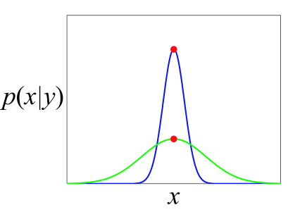
Figure 1: Two posterior distributions with the same MAP estimate but different variances. Decision-making using point estimates but without uncertainty quantification can significantly reduce performance as compared to using the full posterior.

I-A Related work

The full exploitation of Bayesian inference has been developed in a wide range of problems.

Hierarchical Bayesian modeling incorporates priors on the hyper-parameters of the prior distribution to perform high-order statistical modeling and inference [11, 12, 13]. This improves the prediction of a Bayesian model that often depends on the prior distributions. When $X$ is a random process obeying a state-space model (e.g. Markov chain), particle filtering and sequential importance sampling incorporate the dynamics of $X$ [14, 15] to sequentially update posteriors. These sequential Monte Carlo methods recursively compute the relevant probability distributions using ensembles of “particles” and their weights. Nonparametric Bayesian methods, attracting increasing interest, [16, 17, 18, 19], make fewer assumptions on the distributions of interest and allow their parametric complexity to increase with the amount of data acquired.

For the remainder of this manuscript, we will consider the canonical Bayesian inference problem in (1) where $X\subset\mathbb{R}^{d}$, $P_{X}(x)$ has a density $p(x)$ with respect to the Lebesgue measure, and the likelihood model is specified in density form as $p(y|x)$.

For a given likelihood $p(y|x)$, in order to obviate the integration in calculating $\beta_{y}$ in (1), conjugate priors allow for a closed-form expression for the posterior. However, these are very limiting cases and the conjugate prior is often selected only for computational purposes, even if it does not actually represent prior knowledge about $X$.

Markov chain Monte Carlo (MCMC) methods [20, 21, 22, 23, 24] have enabled widespread attempts at fully Bayesian inference by representing a probability distribution as a set of samples and iterating them through a Markov chain whose invariant distribution is the posterior. Despite the wide adoption, MCMC has a few drawbacks: (a) the convergence rates and mixing times of the Markov chains are generally unknown, thus leading to practical shortcomings like “burn in” periods of discarded samples; (b) the samples generated are from a Markov chain and thus necessarily correlated – lowering effective sample sizes and propagating errors throughout estimates as in (3); (c) many different highly specialized, problem-specific variants of MCMC exist, all of which have their own benefits and challenges [20].

Efficient approximation methods, such as variational Bayes [25, 26, 27] and expectation propagation (EP) [28, 29, 30] have been developed. These offer a complementary alternative to sampling methods and have allowed Bayesian techniques to be used in large-scale applications. Variational methods yield deterministic approximations to the posterior distribution. A particular form that has been used with great success is the factorized one [31]. However, these methods are based upon approximations and thus there are no guarantee that the iterations of the approximation methods will converge, or provide exact results in the limit.

I-B Optimal transport framework

Recently, El Moselhy et al. proposed a method to construct a map that pushed forward the prior measure to the posterior measure, casting Bayesian inference as an optimal transport problem [32]. Namely, the constructed map transforms a random variable distributed according to the prior into another random variable distributed according to the posterior. This approach is conceptually different from previous methods, including sampling and approximation methods.

Optimal transport theory has a long and deep history dating back to Monge [33], Kontarovich [34], and most recently Villani [35]. This study of measure preserving maps has its roots and applications in vast areas, spanning resource allocation, dynamical systems, optimal control, and fluid mechanics.

Monge initially stated the “earth movers” problem as finding the cheapest way to move a pile of sand in a specific location and shape, to a different location and shape while maintaining the same volume. While this captures the mass-preserving and optimality criterion of the map, it is worth explaining the effect of the map a little more by way of an example. We can relate the optimal map construction to finding the optimal placement of “pegs” in a Galton board, to transform one distribution of balls into another as shown in Fig. 2. Conceptually, one could imagine searching for a unique beam placement resulting in a different output distribution. For example, Fig. 2 (a) shows the trivial schematic diagram of a map that pushes forward a uniform distribution $P$ to another uniform $Q$, while Fig. 2 (b) pushes forward a uniform $P$ to a Gaussian distribution $Q$.

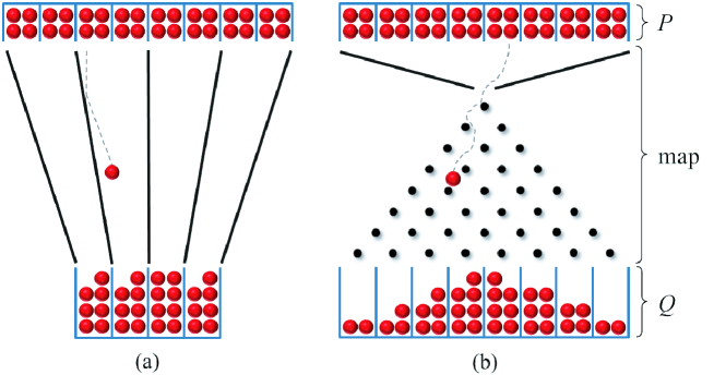
Figure 2: Conceptual explanation of transforming samples from a distribution $P$ to distribution $Q$ through the use of a Galton board. Two different placements provide some intuition for a map-based construction: (a) a uniform to another uniform, and (b) a uniform to a Gaussian.

I-C Our contribution

The use of an optimal transport map for Bayesian inference was proposed in [32] by minimizing the variance of an operator, but it was a non-convex problem – even for the case of log-concavity of prior and likelihood. In [36], we consider the optimal transport map viewpoint established in [32], but we replace variance minimization with an equivalent approach based upon KL divergence minimization. Remarkably, for the case of log-concave priors and likelihoods, we showed this KL divergence minimization is a convex optimization problem and thus tractable.

The rest of the paper is outlined as follows. In section II, we first consider a more general problem: transforming samples from one continuous source distribution into samples from another target distribution. We demonstrate with optimal transport theory that when the source distribution can be easily sampled from and the target distribution is log-concave, a KL divergence minimization procedure yields samples from target distribution with convex optimization. We develop an empirical and truncation approach to computationally approximate the convex problem. We exploit the sub-exponential tail property of log-concave distributions to prove consistency of the proposed scheme in the remainder of this section. In section III, we demonstrate that fully Bayesian inference (e.g. where the source is the prior and target is the posterior) is a special case. Remarkably, we show that the tractability criterion becomes log-concavity of the prior and likelihood in $x$: the same criterion for obtaining tractable MAP estimates in (2). This implies that general purpose frameworks for Bayesian point estimation with convex optimization can be improved to fully Bayesian inference, still with convex optimization. Section IV demonstrate how we can attain the Bayes risk in simulations. With physiologic data, we demonstrate improvements over point estimation in intensive care unit (ICU) outcome prediction and in sleep staging based upon electroencephalography (EEG) recordings. We conclude with a discussion in Section V.

II General push-forward theorem

Before going into the details, we present a general theorem of an optimal map construction to transform a distribution $P$ to another distribution $Q$. We also informally go through an illustrating example. This general push-forward theorem will be used in the Bayesian inference framework in the next section.

II-A Problem setup

We provide a problem setting with notations and definitions relevant to the development of the push-forward theorem where the latent variable is in a continuum. For a set ${\mathsf{X}}\subset\mathbb{R}^{d}$ where $d$ is a positive integer, define the space of all probability measures on ${\mathsf{X}}$ as ${\mathsf{P}}\left({\mathsf{X}}\right)$. Then the push-forward theorem is defined as follows.

Definition II.1 (Push-forward).

Given $P\in{\mathsf{P}}\left({\mathsf{X}}\right)$ and $Q\in{\mathsf{P}}\left({\mathsf{X}}\right)$, we say that the map $S:{\mathsf{X}}\to{\mathsf{X}}$ pushes forward $P$ to $Q$ (denoted as ${S{\#}P=Q}$) if a random variable $U$ with distribution $P$ results in $Z\triangleq S(X)$ having distribution $Q$.

We say that $S:{\mathsf{X}}\to{\mathsf{X}}$ is a diffeomorphism on ${\mathsf{X}}$ if $S$ is invertible and both $S$ and $S^{-1}$ are differentiable. Denote the set of all diffeomorphisms on ${\mathsf{X}}$ as $\mathcal{D}$. With this, we have the following lemma from standard probability:

Lemma II.2.

Consider a diffeomorphism $S\in\mathcal{D}$ and $P$, $Q\in{\mathsf{P}}\left({\mathsf{X}}\right)$ that both have the densities $p$, $q$ with respect to the Lebesgue measure. Then $S_{\#}P=Q$ if and only if

$$p(x)=q(S(x))\left|\det{\left(J_{S}(x)\right)}\right|,\quad\forall x\in{\mathsf{X}}$$ (5)

where $J_{S}(x)$ is the Jacobian matrix of the map $S$ at $x$.

Throughout this section it is worth discussing a simple example:

Example 1.

Let $X\sim P$ where $P$ is a uniform on $[0,2]$, and consider building the transformation $Z=S(X)$ so that $Z\sim Q$ where $Q$ is a uniform on $[0,1]$. The desired transformation is represented by the solid lines in Fig. 3. Note that clearly the maps $S^{*}(x)=\frac{1}{2}x$ and $S^{*}(x)=\frac{1}{2}(2-x)$ transform $P$ to $Q$ and thus satisfy the Jacobian equation (5). One is increasing, the other is decreasing in $x$. Note that there are multiple maps that push $P$ to $Q$. An arbitrary map $S$, e.g., $S(x)=\frac{1}{3}x$, does not necessarily push $P$ to $Q$, but rather pushes some $\tilde{P}\neq P$ to $Q$, namely, $\tilde{P}=\text{unif}[0,3]$. This transformation is represented by the dotted line in Fig. 3.

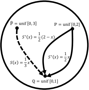
Figure 3: Transformation from a distribution $P=\text{unif}[0,2]$ to $Q=\text{unif}[0,1]$. There are multiple maps $S^{*}$ that push forward $P$ to $Q$: $\frac{1}{2}x$ and $\frac{1}{2}(2-x)$. An arbitrary map $S$ will always push forward some $\tilde{P}$ to the target $Q$, as shown above, but the $\tilde{P}$ does not need to be the $P$ we started from.

Given a fixed density $q$ and an arbitrary diffeomorphism $S$, the corresponding Jacobian equation for the induced density $\tilde{p}_{S}$ is given by

$$\tilde{p}_{S}(x)=q(S(x))|\det\left(J_{S}(x)\right)|,\quad\forall x\in{\mathsf{X}}.$$ (6)

We denote it by $\tilde{p}_{S}$ to make clear that given $q$ and $S$, the associated $\tilde{p}$, which $S$ pushes to $Q$, is functionally dependent upon $S$ through the right hand side of (6). Note that the left-hand side of (5) involves the true $p$ induced by the optimal $S^{*}$, whereas the left-hand side of (6) involves the $\tilde{p}_{S}$ induced by an arbitrary $S$.

Next, we propose an algorithm to find an optimal nonlinear map that satisfies the Jacobian equation in (5) by searching over all possible maps $S$ that push forward some $\tilde{P}_{S}$ to $Q$ given by (6). Finding a map $S^{*}$ that pushes $P$ to $Q$ is equivalent to finding a map $S$ for which the “distance” between $\tilde{P}_{S}$ and $P$ is zero. Using KL divergence, this becomes:

$$\!\!\!D(P\|\tilde{P}_{S}) =\mathbb{E}_{P}\left[\log\frac{p(X)}{\tilde{P}_{S}(X)}\right]$$ (7)

$$=-h(P)+\mathbb{E}_{P}\left[-\log\tilde{p}_{S}(X)\right]$$ (8)

where $h(P)$ is the Shannon differential entropy of $P$[6], which is fixed with respect to $S$. For the remainder of the manuscript, we assume the following:

Assumption 1.

$\mathbb{E}\left[|\log p(X)|\right]<\infty$.

From Jensen’s inequality, Assumption 1 implies $\left|h(P)\right|<\infty$ and so we have:
A $\displaystyle\min_{S\in\mathcal{D}}$ $D\!\left(P\|\tilde{P}_{S}\right)$ $\;\Leftrightarrow\;$ $\displaystyle\max_{S\in\mathcal{D}}\;\;\mathbb{E}_{P}\left[\log\tilde{p}_{S}(X)\right]$
 
We note the following:

Lemma II.3.

$S$ is optimal for problem  A if and only if $S$ pushes $P$ to $Q$.

Proof.

By the definition of the Jacobian equation induced by $S$ in (6), $S$ pushes some $\tilde{P}_{S}$ to $Q$. Assume $\tilde{P}_{S}=P$. Then $D\!\left(P\|\tilde{P}_{S}\right)=0$, and from the non-negativity of KL divergence, we have that $S$ solves Problem  A . Now, assume $S$ is optimal for Problem  A . Note that the KL divergence $D\!\left(P\|\tilde{P}_{S}\right)$ is zero if and only if $P=\tilde{P}_{S}$ and thus $S$ pushes $\tilde{P}_{S}\equiv P$ to $Q$. ∎

Now we note from Example 1 that in general there can be more than one optimal solution, some of which satisfy $\det\left(J_{S}(x)\right)>0$, and others, for which $\det\left(J_{S}(x)\right)<0$. Both maps are equally “as good”. However, from an optimization viewpoint, the search space is so “rich” that this leads to non-convexity in an optimization problem.

II-B A Convex Problem in Infinite Dimensions

We here consider restricting our search to orientation-preserving diffeomorphisms, i.e., ones with positive definite Jacobian:

$$\mathcal{D}_{+}\triangleq\left\{S\in\mathcal{D}:J_{S}(x)\succ 0\;\forall x\in{\mathsf{X}}\right\}.$$ (9)

This eliminates possible maps such as $S^{*}(x)=\frac{1}{2}(2-x)$ in Example 1. As such, for any $S\in\mathcal{D}_{+}$, the Jacobian equation becomes:

$$\tilde{p}_{S}(x)=q(S(x))\det\left(J_{S}(x)\right).$$ (10)

This gives rise to following problem, which simply involves a restriction of the feasible set in Problem  A to orientation-preserving maps:
B $\displaystyle\min_{S\in\mathcal{D}_{+}}$ $D\!\left(P\|\tilde{P}_{S}\right)$ $\;\Leftrightarrow\;$ $\displaystyle\max_{S\in\mathcal{D}_{+}}\;\;\mathbb{E}_{P}\left[\log\tilde{p}_{S}(X)\right]$

With this, we can state the following theorem:

Theorem II.4.

Problem B has an optimal solution $S^{*}$, which is also optimal for Problem  A , and thus pushes $P$ to $Q$.

Proof.

Since $P$ and $Q$ have densities $p$ and $q$ with respect to the Lebesgue measure, we consider the Monge-Kontarovich problem with Euclidean distance cost [35]:

$$\quad\min_{S:{\mathsf{X}}\to{\mathsf{X}}} \int_{x\in{\mathsf{X}}}\|x-S(x)\|^{2}p(x)dx$$

s.t. $${S{\#}P=Q}.$$

Key properties of its optimal solution $S^{*}$ include: (i) $S\in\mathcal{D}$, and (ii) $S^{*}(x)=\nabla h(x)$ where $h$ is a strictly convex function (which implies that $J_{S^{*}}(x)\succ 0$ for all $x\in{\mathsf{X}}$). Thus $S^{*}$ lies in the feasible set of problem  B . But from the Monge-Kantorovich problem, $S^{*}$ pushes $P$ to $Q$ and is thus optimal for Problem  A . Since the feasible set of problem  A contains the feasible set of problem  B , $S^{*}$ is optimal for Problem  B ∎

In Example 1, both $\frac{1}{2}x$ and $\frac{1}{2}(2-x)$ push $P$ to $Q$, but $\frac{1}{2}x$ is increasing and the other is decreasing. Problem B finds a map $S$ whose Jacobian matrix $J_{S}$ is positive definite (e.g., $S(x)=\frac{1}{2}x$). Remarkably, from Theorem II.4, the restriction to monotonicity suffers no loss in optimality. Moreover, for many problems of interest, it guarantees that finding the optimal solution is tractable:

Theorem II.5.

If $\log q(x)$ is concave in $x$, then problem B is a convex optimization problem with a unique optimal solution.

Proof.

Note that if $S,\tilde{S}\in\mathcal{D}_{+}$ then $J_{S},J_{\tilde{S}}\succ 0$. For any $\lambda\in[0,1]$, $J_{\lambda S+(1-\lambda)\tilde{S}}(x)=\lambda J_{S}(x)+(1-\lambda)J_{\tilde{S}}(x)\succ 0$. Thus $\mathcal{D}_{+}$ is convex. Now we note from (10) that

$$\mathbb{E}_{P}\left[\log\tilde{p}_{S}(X)\right]=\int_{{\mathsf{X}}}\left[\log q(S(x))+\log\det(J_{S}(x))\right]p(x)dx.$$

Since $\log\det(\cdot)$ is strictly concave over the space of positive definite matrices and since $\log q(\cdot)$ is concave, we have that $\mathbb{E}_{P}\left[\log\tilde{p}_{S}(X)\right]$ is a sum of strictly convex and convex functions, which itself is strictly convex in $S$. Thus an optimal solution $S^{*}$, which exists from Theorem II.4, is unique. ∎

We make the following remark as it relates to other methods involving KL divergence minimization:

Remark 1.

Variational Bayes [26] and EP [28] methods are also based on the minimization of a KL divergence. However, the KL divergence minimization is of a reverse kind, is not over a space of maps, and is thus conceptually different. Moreover, these methods build upon deterministic approximations to the posterior, do not guarantee exactness, and in general are non-convex.

Although problem  B is convex for log-concave $q$, note that the feasible set is an infinite-dimensional space of functions, and the objective function involves an expectation (e.g. a $d$-dimensional integral) with respect to $P$. Both of these require further effort to be implemented in real computational settings.

II-C A Convex Problem in Finite Dimensions via Truncated Basis

Problem B involves minimizing an expectation with respect to $P$ over $\mathcal{D}_{+}$, an infinite-dimensional space of functions. We here consider representing any $S\in\mathcal{D}_{+}$ in terms of its (truncated) orthogonal basis representation with respect to $P$. We consider maps $m$ of the form:

$$m(x)=\sum_{j\in\mathcal{J}}w_{j}\phi^{(j)}(x)$$ (11)

where $\phi^{(j)}(x)\in\mathbb{R}$ are $d$-variate bases, $w_{j}\in\mathbb{R}^{d}$ are basis coefficients, and $\mathcal{J}$ is a set of all possible indices $j$.

One natural way to do this, if ${\mathsf{X}}\subset\mathbb{R}$, is to perform a polynomial chaos expansion (PCE) of the nonlinear optimal map [37, 38], meaning that we select $(\phi^{(j)}:j\geq 1)$ so that they are orthogonal with respect to $P$:

$$\int_{{\mathsf{X}}}\phi^{(i)}(x)\phi^{(j)}(x)p(x)dx=1_{\left\{i=j\right\}}.$$ (12)

For example, if ${\mathsf{X}}=[-1,1]$ and $P$ is uniformly distributed, then $\phi^{(j)}(x)$ are the Legendre polynomials, and if ${\mathsf{X}}=\mathbb{R}$ and $P$ is Gaussian, then $\phi^{(j)}(x)$ are the Hermite polynomials [37].

Remark 2.

In principle, any basis of polynomials, for which the truncated expansion of functions is dense in the space of all functions on ${\mathsf{X}}$, suffices. Using the PCE where orthogonality is measured with respect to the prior, means that computing conditional expectations and other calculations can be done only with linear algebra.

When $|\mathcal{J}|=K$, we represent a nonlinear map as

$$m(x)=W\Phi(x),\qquad\qquad d\times 1$$ (13)

where $W=[w_{1},\ldots,w_{K}]$ is $d\times K$, and $\Phi(x)=[\phi^{(1)}(x),\ldots,\phi^{(K)}(x)]^{T}$ is $K\times 1$. The Jacobian matrix $J_{m}(x)$ is also expressed as

$$J_{m}(x)=WJ_{\Phi}(x),\qquad\qquad d\times d$$ (14)

where $J_{\Phi}(x)=\left[\partial\phi^{(i)}/\partial x_{j}(x)\right]_{i,j}$ is $K\times d$.

For ${\mathsf{X}}\subset\mathbb{R}^{d}$, a polynomial basis $\phi^{(j)}(x)$ can be represented using tensor products as

$$\phi^{(j)}(x)=\prod_{a=1}^{d}\psi_{j_{a}}(x_{a})$$ (15)

where $\psi_{j_{a}}$ is a univariate polynomial of order $j_{a}$, and $j\to(j_{1},\ldots,j_{d})$ is defined in a standard diagonal manner. For example, if $d=2$, then we have $j\to(j_{1},j_{2})$ where $0\leq j_{1}+j_{2}\leq d$, and thus polynomial bases are given by

$$\begin{array}[]{cc}\phi^{(0)}(x)=\psi_{0}(x_{1})\psi_{0}(x_{2}),&\phi^{(1)}(x)=\psi_{0}(x_{1})\psi_{1}(x_{2}),\\ \phi^{(2)}(x)=\psi_{1}(x_{1})\psi_{0}(x_{2}),&\phi^{(3)}(x)=\psi_{0}(x_{1})\psi_{2}(x_{2}),\\ \phi^{(4)}(x)=\psi_{1}(x_{1})\psi_{1}(x_{2}),&\phi^{(5)}(x)=\psi_{2}(x_{1})\psi_{0}(x_{2}).\end{array}$$ (19)

Since $J_{m}(x)=WJ_{\Phi}(x)$ need not be positive definite, we use the Euclidean projection, or equivalently the proximal operator of the indicator function of $\mathcal{D}_{+}$ [39]:

$$S_{W} = \Pi_{\mathcal{D}_{+}}\left[W\Phi\right]$$ (20)

$$\Pi_{\mathcal{D}_{+}}\left[W\Phi\right](x) \triangleq \!\!\!\!\mathop{\arg\,\!\min}\limits_{m(x)=\tilde{W}\Phi(x):J_{m}(x)\succ 0}\|m(x)-W\Phi(x)\|^{2}.$$

By defining $\mathcal{D}_{+}^{K}\triangleq\left\{S_{W}:W\in\mathbb{R}^{d\times K}\right\}$, we can define the following optimization problem:
C(K) $\displaystyle\min_{S\in\mathcal{D}_{+}^{K}}$ $D\!\left(P\|\tilde{P}_{S}\right)$ $\;\Leftrightarrow\;$ $\displaystyle\max_{S\in\mathcal{D}_{+}^{K}}\;\;\mathbb{E}_{P}\left[\log\tilde{p}_{S}(X)\right]$

We now show that $\mathcal{D}_{+}^{K}\subset\mathcal{D}_{+}$ is dense in $\mathcal{D}_{+}$:

Theorem II.6.

If $q$ is log-concave, then problem  C(K) is a finite dimensional convex optimization problem with a unique optimal solution, which we denote as $S_{K}$. Moreover:

$$\lim_{K\to\infty}D\!\left(P\|\tilde{P}_{S_{K}}\right)=0.$$ (21)

Proof.

Define $S_{\infty}$ to be the unique solution to Problem  B . As such, the random variable $Z=S_{\infty}(X)$ is drawn according to $Q$, which is log-concave. It is well known that any log-concave random variable satisfies the sub-exponential tail property:

$$\mathbb{E}\left[e^{c\left\|{Z}\right\|}\right]<\infty,\quad\text{ for some }c>0.$$

This is a sufficient condition [38, Theorem 3.7] for the tensor products of the generalized polynomial chaos $\Phi_{1}(x),\Phi_{2}(x),\ldots$ to be dense in $L_{2}({\mathsf{X}},\sigma(X),P)$, implying:

$$Z=S_{\infty}(X) \underbrace{=}_{L_{2}}\lim_{K\to\infty}v_{K}(X),$$ (22)

$$v_{K}(X) \triangleq\sum_{i=1}^{K}\langle S_{\infty}(X),\Phi_{i}(X)\rangle\Phi_{i}(X).$$ (23)

Now define

$$\tilde{S}_{K}(X)=\Pi_{\mathcal{D}_{+}}\left[v_{K}\right](X),$$ (24)

and note that

$$\lim_{K\to\infty}\mathbb{E}\left[\|S_{\infty}(X)-\tilde{S}_{K}(X)\|^{2}\right]$$ (25)

$$= \lim_{K\to\infty}\mathbb{E}\left[\|\Pi_{\mathcal{D}_{+}}\left[S_{\infty}\right](X)-\Pi_{\mathcal{D}_{+}}\left[v_{K}\right](X)\|^{2}\right]$$

$$\leq \lim_{K\to\infty}\mathbb{E}\left[\|S_{\infty}(X)-v_{K}(X)\|^{2}\right]$$ (26)

$$= 0$$ (27)

where (25) follows because $S_{\infty}(X)=\Pi_{\mathcal{D}_{+}}\left[S_{\infty}\right](X)$ (since $S_{\infty}\in\mathcal{D}_{+}$) and from (24); (26) follows from the firm non-expansive property of the proximal operator [39]; and (27) follows from (22).

Thus from (27), we have that $\tilde{S}_{K}(X)\to_{L_{2}}S_{\infty}(X)$. Note that $\log q(S_{\infty}(X))+\log\det J_{S_{\infty}}(X)=\log p(X)$ which from Assumption 1 lies in $L_{1}({\mathsf{X}},\sigma(X),P)$. In addition, $\log q(\cdot)$ is concave (and thus continuous), and $\log\det(\cdot)$ is concave (and thus continuous) over the space of positive definite matrices. Since $L_{2}$ convergence implies $L_{1}$ convergence, we have:

$$\log\frac{p(X)}{\tilde{p}_{\tilde{S}_{K}}(X)}\!\!\!\!\!\! = \!\!\!\!\log p(X)-\log q\left(\tilde{S}_{K}(X)\right)-\log\det J_{\tilde{S}_{K}}(X)$$

$$\underbrace{\to}_{L_{1}} \!\!\!\!\log p(X)-\log q\left(S_{\infty}(X)\right)-\log\det J_{S_{\infty}}(X)$$

$$= 0.$$

Since $L_{1}$ convergence implies convergence in distribution, we have that $D\!\left(P\|\tilde{P}_{\tilde{S}_{K}}\right)\to 0$. But since $\tilde{S}_{K}\in\mathcal{D}_{+}^{K}$ and $S_{K}$ is the optimal solution to problem  C(K) , we have that $D\!\left(P\|\tilde{P}_{S_{K}}\right)\leq D\!\left(P\|\tilde{P}_{\tilde{S}_{K}}\right)\to 0$. ∎

II-D Stochastic Convex Optimization in Finite Dimensions

Note that the expectation in problem  C(K) is given as

$$\mathbb{E}_{P}\left[\log\tilde{p}_{S}(X)\right]=\int_{{\mathsf{X}}}\left[\log q(S(x))+\log\det(J_{S}(x))\right]p(x)dx,$$

which cannot in general be evaluated for any $S$. But since this is an expectation with respect to $P$, we can define a probability space $(\Omega,\mathcal{F},\mathbb{P})$ pertaining to i.i.d. samples $(X_{1},X_{2},\ldots)$ drawn from from $P$. We define $P_{n}$ as the empirical distribution on $(X_{1},\ldots,X_{n})$ and then consider the empirical expectation:

$$\mathbb{E}_{P_{n}}\left[\log\tilde{p}_{S}(X)\right]=\frac{1}{n}\sum_{i=1}^{n}\log q(S(X_{i}))+\log\det(J_{S}(X_{i})).$$

This gives rise to a stochastic optimization problem
D(K,n) $\displaystyle\max_{S\in\mathcal{D}_{+}^{K}}\;\;\mathbb{E}_{P_{n}}\left[\log\tilde{p}_{S}(X)\right]$
Since this problem only involves $S(x)$ and $J_{S}(x)$ evaluated at $(X_{1},\ldots,X_{n})$, we can solve this with a multi-step procedure: given i.i.d. $\left(X_{i}\right)_{i=1,N}$ from $P$, evaluate a priori the associated $\left(\Phi_{i}\triangleq\Phi(X_{i})\right)_{i=1,N}$, $\left(J_{i}\triangleq J_{\Phi}(X_{i})\right)_{i=1,N}$. From here, we solve for

$$\max_{W\in\mathbb{R}^{d\times K}} \frac{1}{N}\sum_{i=1}^{N}\log q\left(W\Phi_{i}\right)+\log\det(WJ_{i})$$ (28a)

$$s.t. WJ_{1}\succ 0,\ldots,WJ_{N}\succ 0.$$ (28b)

Given ${W^{*}_{K,n}}$, we employ the proximal operator

$$S^{*}_{K,n}(x)\triangleq S_{{W^{*}_{K,n}}}(x)=\Pi_{\mathcal{D}_{+}}\left[{W^{*}_{K,n}}\Phi\right](x).$$ (29)

so that $S^{*}_{K,n}\in\mathcal{D}_{+}^{K}$.

Remark 3.

Note that Problem  D(K,n) is only tractable if generating i.i.d. samples from $P$ is tractable. Luckily, $P$ in many situations is a well-defined distribution that can be sampled from easily, such as Gaussian, exponential family, uniform, or sum of Gaussians. More generally, if $p(x)$ is log-concave, then we can do as follows: simply first solve an auxiliary Problem $\overline{\text{ {\bf D(K,n)} }}$ with $\bar{P}=\text{uniform}$ or $\bar{P}=\mathcal{N}(0,\Sigma)$, or any other distribution we can easily sample from. Then define $\bar{Q}=P$. By implementing problem $\overline{\text{ {\bf D(K,n)} }}$, we will generate a map $\bar{S}$ that can transform i.i.d. samples from $\bar{P}$, which is easy to sample from, into i.i.d. samples from $P$. From here, we can move forward and implement Problem ${\bf D(K,n)}$ to generate a map $S$ to push $P$ to $Q$.

This optimization problem can be implemented with convex optimization software such as CVX in MATLAB, CVXPY in Python, etc. Here, we implemented the algorithms with CVX [40] in MATLAB.

Theorem II.7.

The map $S^{*}_{K,n}$ as defined in (29) is the unique minimizer of problem  D(K,n) and moreover,

$$\lim_{K\to\infty}\lim_{n\to\infty}D\!\left(P\|\tilde{P}_{S^{*}_{K,n}}\right)=0\quad\mathbb{P}-a.s.$$ (30)

Proof.

The uniqueness of the minimizer follows from strict concavity of the problem. That $S^{*}_{K,n}$ is the minimizer follows because

$$S^{*}_{K,n}(X_{i})=\Pi_{\mathcal{D}_{+}}\left[{W^{*}_{K,n}}\Phi\right](X_{i})={W^{*}_{K,n}}\Phi(X_{i}),\;\;i=1,\ldots,n$$

because the positive definite constraint was imposed on ${W^{*}_{K,n}}$ in the feasible set of the problem in (28). Thus $S^{*}_{K,n}$ corresponds to an optimal solution of the optimization problem defined in (28), which is a relaxation to problem  D(K,n) : they have the same objective but the feasible set of the problem in (28) contains the feasible set in D(K,n) . Since $S^{*}_{K,n}$ solves the relaxation, it solves the original problem.

Now, we can prove (30). Note that for any $S=\Pi_{\mathcal{D}_{+}}\left[W\Phi\right]\in\mathcal{D}_{+}^{K}$ and $S^{\prime}=\Pi_{\mathcal{D}_{+}}\left[W^{\prime}\Phi\right]\in\mathcal{D}_{+}^{K}$, we have

$$\|S-S^{\prime}\|^{2}_{P} = \int_{{\mathsf{X}}}\|\Pi_{\mathcal{D}_{+}}\left[W\Phi\right](x)-\Pi_{\mathcal{D}_{+}}\left[W^{\prime}\Phi\right](x)\|^{2}p(x)dx$$

$$\leq \int_{{\mathsf{X}}}\|W\Phi(x)-W^{\prime}\Phi(x)\|^{2}p(x)dx$$

$$= \int_{{\mathsf{X}}}\|(W-W^{\prime})\Phi(x)\|^{2}p(x)dx$$

$$= \int_{{\mathsf{X}}}\Phi(x)^{T}(W-W^{\prime})^{T}(W-W^{\prime})\Phi(x)p(x)dx$$

$$= \|W-W^{\prime}\|_{P}^{2}$$ (32)

where (II-D) follows from the firm non-expansive property of the proximal operator [39]; and (32) follows from the fact that $\Phi$ is a $P$-orthonormal matrix. Now since $W,W^{\prime}\in\mathbb{R}^{d\times K}$, from (32), we have that with $\mathcal{D}_{+}^{K}$ is locally compact. Thus we can exploit the strict convexity of problem  D(K,n) over a locally compact constraint set and Assumption 1 to conclude [41, Theorem 3.1] that $\mathbb{P}\left(\lim_{n\to\infty}S^{*}_{K,n}=S^{*}_{K}\right)=1$.

With this, we have that

$$\lim_{n\to\infty}D\!\left(P\|\tilde{P}_{S^{*}_{K,n}}\right)=D\!\left(P\|\tilde{P}_{S^{*}_{K}}\right)\quad\mathbb{P}-a.s.$$

By taking an outer limit in $K$, we complete the proof. ∎

III Optimal Transport and Bayesian Inference

In this section, we apply the general push-forward theorem to the context of Bayesian inference. We demonstrate that for a large class of prior and likelihood families, an optimal map can be efficiently constructed through convex optimization.

We assume that $X\in\mathbb{R}^{d}$ is drawn a priori according to $P_{X}$, which has a density $p_{X}(x)$ with respect to Lebesgue measure. We define the likelihood function in density form as $p_{Y|X}(y|x)$. Having observed $Y=y$, the posterior distribution $P_{X|Y=y}$ has a density given by $p_{X|Y=y}(x|y)$, determined by Bayes’ rule in (1). In general, the calculation of $\beta_{y}$ is intractable, especially when $d$ is in high dimension or $p_{X}(x)$ is not a conjugate prior for $p_{Y|X}(y|x)$. Several methods have been developed to bypass its calculation or approximate different functions of the posterior. Typical approaches to perform this are Monte Carlo methods [24]. MCMC methods are families where samples are drawn from a Markov chain, whose invariant distribution is that of the posterior. As described in Section I, one problem of these methods is that because samples are drawn from a Markov chain, they are necessarily statistically dependent; so the law of averages kicks in more slowly. Also, efficient MCMC methods are typically tailored to the specifics of the prior and likelihood and as such, lack generality. In addition, many natural situations require the calculation of $\beta_{y}$, such as information gain calculations mentioned in (4).

III-A Problem Setup

To make use of the general push-forward theorem, we set $P=P_{X}$ as the prior distribution $Q=P_{X|Y=y}$ as the posterior distribution. Then we can find a diffeomorphism $S_{y}^{*}$, for which $S_{y}^{*}\#P=Q$, or equivalently $S_{y}^{*}\#P_{X}=P_{X|Y=y}$. In this Bayesian inference framework, we denote the optimal map $S^{*}$ as $S_{y}^{*}$ with a subscript $y$, since a map depends on each observation $y$. The Jacobian equation for orientation-preserving maps (10) within the context of Bayes’ rule (1) becomes

$$p_{X}(x)=\frac{p_{Y|X}(y|S^{*}_{y}(x))p_{X}\left(S^{*}_{y}(x)\right)}{\beta_{y}}\det{\left(J_{S^{*}_{y}}(x)\right)}.$$ (33)

Next, we (a) exchange $p_{X}(x)$ in the left-hand side of (33) with $\beta_{y}$ in the right-hand side in order to put all the $x$-dependent terms to the right-hand side and (b) take the logarithm and use an arbitrary map $S_{y}(x)$, to define the operator $T:\mathcal{D}_{+}\times{\mathsf{X}}\to\mathbb{R}$ as in [32]:

$$T(S,x) \triangleq\log p_{Y|X}(y|S(x))+\log p_{X}\left(S(x)\right)$$

$$+\log\det\left(J_{S}(x)\right)-\log p_{X}(x).$$ (34)

Using (34), we can now state (33) equivalently as follows.

Lemma III.1.

A diffeomorphism $S^{*}_{y}$ satisfies ${S_{y}^{*}{\#}P_{X}=P_{X|Y=y}}$ if and only if

$$T(S_{y}^{*},x)\equiv\log\beta_{y},\quad\forall x\in{\mathsf{X}}.$$ (35)

Note that this encodes a variational principle. The left-hand side of (35) is allowed to vary with $x$. But for $S^{*}_{y}$, at any $x$, $T(S_{y}^{*},x)$ takes on the same value. Thus this suggests a particular problem formulation[32]:

$$\qquad S_{y}^{*} =\mathop{\arg\,\!\min}\limits_{S_{y}\in\mathcal{D}_{+}}V_{1}(S_{y}),$$ (36)

$$V_{1}(S_{y}) \triangleq\int_{x\in{\mathsf{X}}}\left(T(S_{y},x)-\mathbb{E}[T(S_{y},X)]\right)^{2}p_{X}(x)dx.$$

Remark 4.

Attempting to solve this problem is in general computationally intractable. If we approximate a diffeomorphism decision variable $S_{y}$ using a truncated basis expansion (e.g. PCE), the above problem is still non-convex for log-concave priors and likelihoods. This follows because under log concavity, $T(S,X)$ is concave in $S$, but quadratic functions of differences of concave functions are in general non-convex.

Our insight is to abandon the approach espoused in [32] and instead focus on a subset of common problems with log-concave structure, using an alternative KL divergence based criterion. This leads to a computationally tractable algorithm via convex optimization.

III-B A convex problem

We now show that for many natural priors and likelihoods we can efficiently find a diffeomorphism $S_{y}^{*}$, for which ${S_{y}^{*}{\#}P_{X}=P_{X|Y=y}}$, using an alternative optimality criterion described in Section II. Consider any other diffeomorphism $S_{y}(x)$ that induces some $\tilde{P}_{X}$ whose density is denoted as $\tilde{p}_{X}(x)$. From the modified Jacobian equation (33):

$$\tilde{p}_{X}(x)=\frac{p_{Y|X}(y|S_{y}(x))p_{X}\left(S_{y}(x)\right)}{\beta_{y}}\det{\left(J_{S_{y}}(x)\right)}.$$ (37)

By careful inspection of (37) and (34), we then have that

$$\log\frac{p_{X}(x)}{\tilde{p}_{X}(x)}=\log\beta_{y}-T(S_{y},x).$$ (38)

So if a diffeomorphism $S_{y}^{*}$ satisfies $S_{y}^{*}\#P_{X}=P_{X|Y=y}$, then $p_{X}(x)=\tilde{p}_{X}(x)$, which means

$$0=\log\beta_{y}-T(S^{*}_{y},x)\Leftrightarrow T(S^{*}_{y},x)=\log\beta_{y},\;\;\forall x\in{\mathsf{X}}.$$ (39)

Thus we find a map to minimize the KL-divergence between $P_{X}$ and $\tilde{P}_{X}$, which is given by

$$D\!\left(P_{X}\|\tilde{P}_{X}\right)=\log\beta_{y}-\int_{x\in{\mathsf{X}}}p_{X}(x)T(S_{y},x)dx.$$

This suggests the following optimization problem, equivalent to B in Section II for $P=P_{X}$ and $Q=P_{X|Y=y}$:

$$\qquad S_{y}^{*} = \mathop{\arg\,\!\max}\limits_{S_{y}\in\mathcal{D}{X}}\int_{x\in{\mathsf{X}}}p_{X}(x)T(S_{y},x)dx.$$ (40)

Also note that once we have solved for $S_{y}^{*}$ in (40), we in addition can obtain $\beta_{y}$ by virtue of evalution of the $T$ operator using any $x\in{\mathsf{X}}$ in (35). This is fundamentally the optimization problem we aim to solve for Bayesian inference. By phrasing the inference problem as an optimal transport problem along with the natural assumption of log-concavity of the prior and likelihood, we can create a computationally efficient method to carry out Bayesian inference via convex optimization.

III-C Implementation

Applying the PCE in (11) to approximate the function $S(x)$, we re-define $T(S,x)$ in (34) as

$$\tilde{T}(W,x) \triangleq\log p_{Y|X}(y|W\Phi(x))+\log p_{X}\left(W\Phi(x)\right)$$

$$+\log\det(WJ_{A}(x))-\log p_{X}(x).$$ (41)

By truncating the PCE and approximating the expectation by a weighted sum of i.i.d. samples, we finally arrive at the computationally tractable convex inference problem for Bayesian inference:

$$\qquad W^{*} =\mathop{\arg\,\!\max}\limits_{W\in\mathbb{R}^{d\times K}}\frac{1}{N}\sum_{i=1}^{N}[\log p_{Y|X}(y|W\Phi(X_{i}))$$

$$\quad+\log p_{X}\left(W\Phi(X_{i})\right)+\log\det(WJ_{A}(X_{i}))]$$

$$\text{s.t.}\;\;WJ_{A}(X_{1})\succ 0,\ldots,WJ_{A}(X_{N})\succ 0$$ (42)

where $X_{1},X_{2},\ldots,X_{N}$ are i.i.d. samples drawn from $P_{X}$.

Lemma III.2.

If $p_{X}(x)$ is log-concave and $p_{Y|X}(y|x)$ is log-concave in $x$, then $p_{X|Y=y}(x|y)$ is log-concave and the problem (42) is a convex optimization problem.

Proof.

That $p_{X|Y=y}(x|y)$ is log-concave in $x$ is trivial: it follows directly from the assumption that $p_{X}(x)$ and $p_{X|Y=y}(x|y)$ are log-concave in $x$, along with Bayes’ rule (1). As for showing that $\tilde{T}(W,x)$ is concave in $W$, this follows from (i) the assumption that $p_{X}(x)$ and $p_{X|Y=y}(x|y)$ are log-concave in $x$; and (ii) that concavity is preserved under affine transformations ($W\to W\Phi(x)$, $W\to WJ_{A}(x)$)[42]. As for the feasible set, a set of vectors satisfying an affine positive definite constraint is convex [42]. ∎

IV Results

This section demonstrates how the proposed method was applied in several examples. Firstly, we tested the accuracy of the proposed method using a conjugate distribution where the closed-form expression of the posterior is known. Next, we considered several Bayesian inference problems using simulated and real data. Table I summarizes the basic settings of these problems in terms of observations, unknown parameters, likelihoods, and priors. As described, we considered Gaussian likelihoods with a sparse (Lapacian or exponential) prior; and logistic regression likelihoods with a Gaussian prior. We considered many fully Bayesian scenarios, including sampling from the posterior, estimating Bayesian credible regions, and risk minimization. We compare performance to point estimation counterparts by comparing expected losses and by comparing receiver operating characteristic (ROC) curves. For the sake of brevity, we denote the densities, $p_{X}(x)$, $p_{Y|X}(y|x)$, and $p_{X|Y=y}(x|y)$ as $p(x)$, $p(y|x)$, and $p(x|y)$, respectively.

TABLE I: Summary of problem settings in Section IV: 1) Gaussian likelihood with sparse prior (Laplace or exponential for $\mathbf{x}>0$); and 2) Logistic regression with Gaussian prior.

Settings Gauss $\times$ Laplace Logis Reg $\times$ Gauss $\mathbf{Y}$, $\mathbf{X}$ $\mathbb{R}^{d}$, $\mathbb{R}^{d}$ $\mathbb{R}^{d}$, $\mathbb{R}^{d}$ $-\log P_{\mathbf{Y}|\mathbf{X}}(\mathbf{y}|\mathbf{x})$ $\propto||\mathbf{y}-\mathbf{Mx}||_{2}^{2}$ $\log(1+e^{\mathbf{x}^{\text{T}}\mathbf{y}})-c\mathbf{x}^{\text{T}}\mathbf{y}$ $-\log P_{\mathbf{X}}(\mathbf{x})$ $\propto||\mathbf{x}||_{1}$ $\propto||\mathbf{x}||_{2}^{2}$

IV-A Conjugate distribution: comparison to closed-form

We demonstrate how accurately the proposed algorithm can construct a map using the conjugate distribution where the posterior has the same form as the prior and could be expressed as closed-form. In this example, we chose a Poisson likelihood function (where ${\mathsf{Y}}=\left\{0,1,\ldots\right\}$) and its corresponding conjugate prior, a Gamma distribution (where ${\mathsf{X}}=[0,\infty)$).

When we have a Poisson likelihood expressed by $p(y|x)=x^{y}e^{-x}/y!$ and its conjugate Gamma prior expressed by $p(x)=1/(\Gamma(a)b^{a})x^{a-1}e^{-x/b}$, then the posterior, $p(x|y)$, is computed as the Gamma distribution, which is given by

$$p(x|y)\propto x^{a+y-1}e^{-(b+1)/bx}.$$ (43)

That is, the hyper-parameters in the Gamma prior, $a$ and $b$, are changed as $a+y$ and $b/(b+1)$ in the Gamma posterior. In this simulation, we set $a=2$ and $b=0.5$, and specified an observation $y=1$. We then designed multiple maps to push forward the Gamma prior to the Gamma posterior by changing the number of i.i.d. samples, $N$, drawn from the Gamma prior. We chose the number of maximum order of the polynomial in (11) to be 5, resulting in $K=6$.

We then tested the accuracy of the constructed optimal map. The solid line in Fig. 4 plots the variance of $\tilde{T}(W,x)$ in the log-scale. For the optimal parameter $W^{*}$, $\tilde{T}(W^{*},x)$ is almost constant over $x$, so the variance is close to zero. We also computed the KL-divergence between the original prior, $P_{X}$, and the map-dependent prior, $\tilde{P}_{S^{*}}$, estimated using the designed map, shown by the dotted line. As shown, the accuracy increases in both cases as we increase the number of i.i.d. samples we used for the construction.

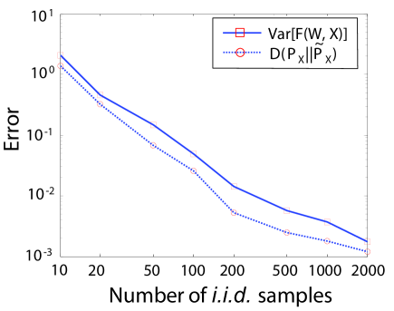
Figure 4: Conjugate distribution problem. The variance of $\tilde{T}(W,x)$ and the KL-divergence between $P$ and $\tilde{P}_{S^{*}}$ decreased with the number $n$ of i.i.d. samples drawn from the prior.

Fig. 5 illustrates the actual transformation of the Gamma prior to the Gamma posterior. The curve inside the plot represents the designed optimal map, constructed using $N=1000$ i.i.d. samples. The curve on the $y$-axis represents the true posterior, $p(x|y)$, in (43). The histogram on the $y$-axis was generated using the posterior samples that were obtained by transforming the prior samples on the $x$-axis through the designed map, $S_{y}^{*}(x)=\Pi_{\mathcal{D}_{+}}\left[W^{*}\Phi\right](x)$. The true posterior, $p(x|y)$, matched well with the histogram of the posterior samples obtained using the designed map. This demonstrated that the proposed method constructed the desired map accurately. We also emphasize that it is straightforward to generate samples from the posterior distribution by transforming samples drawn from the prior distribution - which is usually easy to sample from.

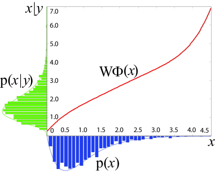
Figure 5: Illustration of the transformation of a prior, $p(x)$, to a posterior, $p(x|y)$. The red curve represents a designed nonlinear optimal map to push forward the prior on the $x$-axis to the posterior on the $y$-axis.

IV-B Bayesian Credible Region

In statistics, point estimates give a single value, which serves as the best estimate of an unknown parameter. For example, we can calculate the mean of samples, or estimate a value to maximize the likelihood or the posterior of the unknown parameter. However, point estimates have several drawbacks, a major one of which is that they do not provide any uncertainty measure of their estimate. It is often important to know how reliable our estimate is in many applications, and thus is desirable to calculate an interval estimate (called Bayesian credible region), within which we believe the unknown population parameter lies with high probability.

The Bayesian credible region is not uniquely defined, and there are several ways to define it: choosing the narrowest region including the mode, choosing a central region where there exists an equal mass in each tail, choosing a highest probability region, all the points outside of which have a lower probability density, etc. However, it is generally tricky to obtain these credible regions in high dimensions, even though we can compute the posterior distribution. In this paper, we introduce two approaches to compute credible regions using the designed optimal map.

First, in order to compute the (1-$\alpha$) credible region of the posterior where $0\leq\alpha\leq 1$, we obtain a region of the prior, within which (1-$\alpha$) of the prior probability mass is contained. We call this region the region with (1-$\alpha$) confidence. The region of the prior with (1-$\alpha$) confidence is generally easy to obtain; for instance, for a $d$-dimensional Gaussian prior with zero mean and $\sigma^{2}$ variance, we choose the region with (1-$\alpha$) confidence as the $d$-sphere with $r_{\alpha}$ radius where $r_{\alpha}$ satisfies $P(\|\mathbf{X}\|_{2}^{2}\leq r_{\alpha}^{2})=1-\alpha$. Since $\|\mathbf{X}\|_{2}^{2}\sim\sigma^{2}\chi^{2}_{d}$ where $\chi^{2}_{d}$ represents the Chi-squared distribution with $d$ degrees of freedom, we can compute $r_{\alpha}^{2}/\sigma^{2}$, above which $\chi^{2}_{d}$ has its $\alpha$ probability mass. Then, it is straightforward to compute the (1-$\alpha$) credible region of the posterior distribution by transforming this $d$-sphere through the designed optimal map.

To help illustrate this approach, we go through an example as follows. Suppose that we have a binary class dataset as shown in Fig. 7 where a red plus sign represents samples from one class, and a blue circle from the other. We denote samples (or regressors) in the 2-dimensional space by $\mathbf{y}_{i}=[y_{i,1},y_{i,2}]^{\text{T}}$, unknown parameters of the logistic regression by $\mathbf{x}=[x_{1},x_{2}]^{\text{T}}$, and the class label corresponding to the $i$th sample $\mathbf{y}_{i}$ by $c_{i}\in\{0,1\}$. Then, the logistic regression likelihood function is given by $p(\mathbf{y}|\mathbf{x})=\prod_{i}p(c_{i},\mathbf{y}_{i}|\mathbf{x})$ where a logistic regression model is $p(c=1,\mathbf{y}|\mathbf{x})=e^{{\mathbf{x}^{\text{T}}\mathbf{y}}}/(1+e^{{\mathbf{x}^{\text{T}}\mathbf{y}}})$ for $c=1$, and $p(c=0,\mathbf{y}|\mathbf{x})=1-p(c=1,\mathbf{y}|\mathbf{x})$ for $c_{i}=0$. We model a prior on $\mathbf{X}$ using a Gaussian distribution with zero mean and 100 variance to regularize the problem. Although both the prior and likelihood functions are log-concave over ${\mathsf{X}}$, there is no closed-form expression of the posterior distribution; thus, we constructed an optimal map to transform the prior to the posterior.

The big circle in Fig. 6 (a) illustrates the region with 95 $\%$ confidence for Gaussian prior in 2-d space. This region was obtained using the method described above. Fig. 6 (b) illustrates the Bayesian credible regions obtained by transforming the region with 95 $\%$ confidence of the prior in (a) through the designed optimal map. The 95 $\%$ credible regions in Fig. 7 (c) and (d) were also obtained in the same manner.

Secondly, we describe another approach to obtain Bayesian credible regions using the i.i.d. samples drawn from the posterior. Once we design the optimal map, it is straightforward to generate i.i.d. samples drawn from the posterior by transforming i.i.d. samples drawn from the prior. For example, the scatter plots in Fig. 6 (a) and (b) show 2000 i.i.d. samples drawn from the prior and the posterior, respectively; The samples in (b) were generated by transforming the samples in (a) through the optimal map. Then we can find the credible interval for each parameter, within which the (1-$\alpha$) portion of the samples is contained. The solid vertical and horizontal lines in Fig. 6 (b) represent 95 $\%$ central regions where there exist 5 $\%$ of total samples (50 samples) in both tails.

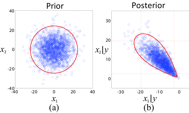
Figure 6: Transformation of confidence regions of prior to credible regions of posterior using designed optimal map. (a) Region of Gaussian prior with 95 $\%$ confidence is illustrated by the circle. 2,000 i.i.d. samples drawn from prior are scatter-plotted together. (b) Bayesian credible regions with 95 $\%$ confidence is illustrated by fan shape. 2,000 i.i.d. samples drawn from posterior are scatter-plotted together. The vertical and horizontal lines also represent the 95 $\%$ credible region for the marginal distribution of each parameter.

Next, using the proposed method we obtained Bayesian credible regions of two datasets in binary classes as shown in Fig. 7 (a) and (b), respectively. The dataset in Fig. 7 (a) included 100 samples from each class, and the dataset in Fig. 7 (b) has 2 samples for each class. Red plus signs represent samples belonging to one class, and blue circles to the other. The MAP estimates of $x$ of both datasets are same as illustrated as the dots at $(-3.9,3.9)$ in Fig. 7 (c) and (d). Although the samples in the two datasets had very different numbers and were differently distributed, MAP estimation provided us with an identical inference of the unknown parameters.

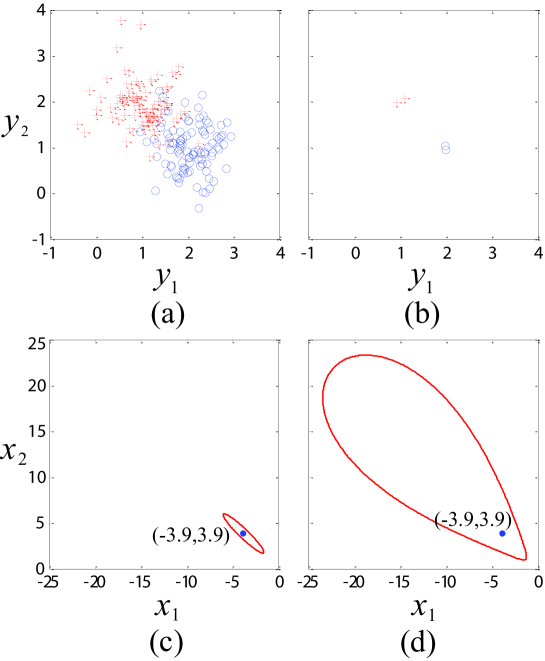
Figure 7: (a) Binary-class data with $200$ samples. (b) Binary-class data with $4$ samples. (c) $95\%$ Bayesian credible region (within red line) with an MAP point estimate (blue point) using the data in (a). (d) $95\%$ Bayesian credible region with an MAP point estimate using the data in (b).

In addition to the point estimate, we obtained the Bayesian credible region as a measure of confidence, as illustrated by the red contours in Fig. 7 (c) and (d). Although we obtained identical MAP estimates from both datasets, we had very different credible regions. The dataset in Fig. 7 (a) with 200 samples provided us much smaller credible region than the dataset in Fig. 7 (b) with 4 samples, meaning that we were more confident on the estimate obtained using the dataset in Fig. 7 (a). There exists more variability in the direction of quadrant II in both datasets, and of course, we can see much more variability for the dataset in Fig. 7 (b). There is less variability in the direction of quadrant IV, since the parameters in quadrant IV switch the classification result.

IV-C Bayes Risk

So far we have demonstrated how we can compute the posterior probability of an unknown parameter and use it to quantify the degree of uncertainty. In other situations, we perform Bayesian inference for the purpose of taking some action. What action is taken can depend on the estimate of some unknown parameter $x\in{\mathsf{X}}$, our estimate of an unknown label $c\in\mathsf{C}$ of an observation, etc. Here, we demonstrate how an action can be improved when using the computed posterior as compared to when using point estimates (e.g. MAP).

Suppose that we take some action $a\in\mathsf{A}$ based on an unobserved parameter $x$ (or a label $c$) given some observation $y\in Y$. As a general method to measure the performance of this action, we define a loss function $l(a,x)$, (or $l(a,c)$), which quantifies the quality of the action $a$ as it relates to the true outcome $x$ (or $c$). It is well known that the procedure to minimize expected loss, attaining the Bayes risk, uses the posterior distribution as follows

$$a^{*}(y)=\arg\underset{a\in\mathsf{A}}{\min}\;\int_{x}p(x|y)l(a,x)dx.$$ (44)

Equation (44) tells us how to devise an optimal action, but it’s generally not easy to solve because it’s difficult to perform computation over the posterior distribution $p(x|y)$. In special cases, there exist corresponding optimal actions for particular loss functions: the MAP estimate for the 0-1 loss, the posterior mean for the squared loss, and the posterior median for the absolute loss. These are special Bayesian estimates for certain loss functions where point estimates can provide us the optimal action, but for an arbitrary loss function we need to solve the optimization problem based on (44), which is usually challenging. We address these challenges using our Bayesian inference method.

For binary decision problems considered in this paper, we also used the receiver operating characteristic (ROC) curve to visualize the performance across different balances of type-I and type-II errors.

In the following subsections, we demonstrate how our Bayesian inference method can be used to help devise an optimal action given observations using simulation and real data.

IV-D Simulation

Firstly, we applied this framework to design an optimal action in the context of sparse signal representations using simulation data. Suppose that our observation $\mathbf{y}\in\mathbb{R}^{m}$ is given as a noisy measurement of a linear forward model. The standard form of this problem is expressed by

$$\mathbf{y}=\mathbf{MX}+\mathbf{e}$$ (45)

where $\mathbf{X}\in\mathbb{R}^{d}$ is the vector of parameters that are sparse, $\mathbf{M}\in\mathbb{R}^{m\times d}$ is a matrix for the linear forward model, and $\mathbf{e}\in\mathbb{R}^{m}$ is noise. This simple model appears in many guises: sparse signal separation where $\mathbf{M}$ is a mixing matrix [43, 44], and sparse signal representation using overcomplete dictionaries where $\mathbf{M}$ is a basis matrix whose columns represent a possible basis [45], to name a few. In this example, we set $m=3$ and $d=3$. To impose the sparsity model on $\mathbf{X}$, we assumed that the parameters $\mathbf{X}$ are endowed with a Laplace prior, $p(\mathbf{x})\propto\exp(-||\mathbf{x}||_{1}/b)$, and the noise $\mathbf{e}$ is assumed to be Gaussian with a zero mean, $\mathbf{e}\sim N(0,\Sigma_{e})$. We randomly generated the forward model $\mathbf{M}\in\mathbb{R}^{3\times 3}$ from a Gaussian distribution, and also set the variance parameters for the prior and the measurement noise as $b=1/\sqrt{2}$ and $\Sigma_{e}=0.1I$, respectively.

Given this setting, we aimed to decide whether each component of the true parameter $\mathbf{x}$ was greater than a preset threshold $\tau>0$ or not based on the computed posterior and the MAP estimate, respectively. To achieve this, we designed a loss function as $l(\mathbf{a},\mathbf{x})=\sum_{i=j}^{3}l(a_{j},x_{j})$ where $l(a_{j},x_{j})=1$ was 1 if we made an incorrect decision; that is, $a_{j}=1$ and $|x_{j}|<\tau$, or $a_{j}=0$ and $|x_{j}|>\tau$. Otherwise, if the decision was correct, the loss function was zero. Here, $\tau$ was chosen to contain 95 $\%$ of the prior density’s mass.

For each simulation, we randomly generated a new $\mathbf{M}$, $\mathbf{X}$, and $\mathbf{e}$. To devise a Bayesian optimal decision, we first approximated the expected loss in (44) as (3), using the posterior samples $Z_{i}$ drawn from $p(x|y)$ using the designed optimal map. Then we found $\mathbf{a}$ to minimize the computed expected loss for each simulation. For MAP decision, we simply performed

$$a^{*}_{MAP}=\mathop{\arg\,\!\min}\limits_{a=\{0,1\}}l(a,\mathbf{x}_{\text{MAP}}).$$ (46)

Thus the MAP decision was made as $a^{*}_{MAP}=1$ if $|x_{\text{MAP}}|>\tau$ and $a^{*}_{MAP}=0$ otherwise. Then we computed losses of both decisions by comparing them to the true $x$ that was used to generate the observation $y$. We repeated these simulations 200 times. The Bayes decision rule made no incorrect decisions for all 200 simulations, but the MAP decision incurred the losses 0, 1, 2, and 3 for 112, 71, 15, and 2 simulations, respectively.

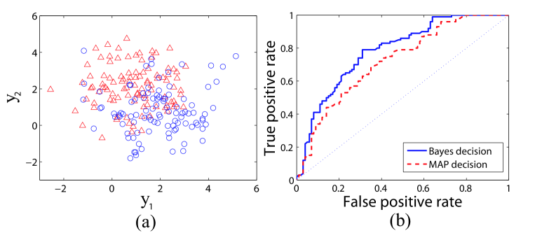
Figure 8: Performance comparison between Bayes and MAP decisions. (a) Scatter plot of 100 input variables for test. (b) ROC curves for Bayes and MAP decisions for Bayesian logistic regression problem with Gaussian prior.

Secondly, we applied this framework to the context of logistic regression using the simulation data $y$ in binary classes as described in the third column of Table I. Logistic regression has been widely used in many applications, since it is usually simple and fast to fit a model to data and easy to interpret the resulting model. In many applications, it is useful to compute the posterior distribution of the parameters for logistic regression model. However, there is no conjugate prior, so posterior calculations can be challenging. Although the posterior is often approximated as Gaussian, it can deviate much from the true posterior, due to asymmetry as shown in Fig. 7 (d). In this example, we instead computed the posterior distribution for logistic regression using our proposed Bayesian method.

We demonstrated that the computed posterior helped make a better decision than an MAP point estimate using samples for a binary decision problem. We first computed the conditional probability of a label given observation, $p(c|y)$, and then obtained the ROC curves by comparing the computed $p(c|y)$ to varying decision thresholds. The conditional probability is given as $p(c|y)=\int_{x}p(c|x,y)p(x|y)dx$ where $p(c|x,y)$ is in the form of sigmoid function. For Bayesian decision, $p(c|y)$ is approximated by $1/n\sum_{i=1}^{n}p(c|Z_{i},y)$ using $Z_{i}$ drawn from $p(x|y)$. For the MAP decision, $p(c|y)$ is approximated by $p(c|x_{\text{MAP}},y)$. We used 10 samples (5 in each class) to compute the posterior and its MAP estimate. Then we tested Bayes and MAP decisions using new 100 samples (50 samples in each class) generated from the same distribution, which were plotted in Fig. 8 (a). The Gaussian prior with zero mean and unit variance was used. The ROC curve in Fig. 8 (b) illustrates that the Bayes decision showed a better decision performance than the MAP decision.

IV-E Real data

Here, we applied the proposed Bayesian inference framework to real data sets such as EEG recordings for sleep study [46] and physiological measurements from ICU patients.

Firstly, we demonstrate how we estimated the Fourier magnitude representation of EEG recordings for sleep scoring from a Bayesian perspective, and then how we used this representation to improve a sleep monitoring system. Existing methods for sleep scoring analyzed the relationship of the activity of frequency bands with sleep stages [47]. So they relied on the power spectrum estimate of EEG recording, but largely ignored how reliable this estimate was. From a statistical viewpoint, the Fourier representation of a signal can be interpreted as the maximum likelihood (ML) estimate under a Gaussian noise with zero mean, and tends to produce many small weights across all frequencies. However, a sleep EEG signal has special time-frequency structure, i.e., its power spectrum tends to concentrate on a certain band or sub-bands depending on sleep stages, so the standard Fourier transform based approach for sleep monitoring may not always be an optimal representation for sleep staging. To address this issue, we put a sparse prior on the Fourier magnitude spectrum. By applying an appropriate prior on the average magnitude spectrum, the spectral analysis in the Bayesian perspective provides us not only a better representation of the power spectrum, but also an additional information on our uncertainty on these estimates. This allows for an opportunity to design a better automatic sleep scoring system.

For the Bayesian spectrum analysis we used PhysioNet[48] sleep EEG recording which provides the recordings together with their hypnograms (a graph that represents the sleep stages as a function of time) that sleep experts annotated, and we used these hypnograms as the ground truth of the decision test. We divided the full-band EEG signal into 8 sub-band ones to characterize the sleep EEG signal in terms of the power in each sub-band. A set to include all the frequency components in the $i$th sub-band was denoted as $\mathbb{F}_{i}$ for $i=1,2,...,8$. The sets, $\mathbb{F}_{1}$, $\mathbb{F}_{2}$, and $\mathbb{F}_{3}$ covered delta (0.5-4 Hz), theta (4-8 Hz), and alpha (8-12 Hz) bands, $\mathbb{F}_{4}$ and $\mathbb{F}_{5}$ covered beta (12-35 Hz) together, and $\mathbb{F}_{6}$, $\mathbb{F}_{7}$, and $\mathbb{F}_{8}$ covered the high frequency band (35-50 Hz), respectively. The sampling frequency was 100 Hz.

The problem settings were described in Table I. We then computed the posterior distribution of the averaged magnitudes in each sub-band. Suppose that $y_{k}$ represented the $k$th Fourier component of noisy EEG recording with an additive Gaussian noise with zero mean and $\sigma^{2}$ variance, and $x_{k}$ represented the Fourier magnitude of the original EEG signal before the noise was added. That is, $y_{k}$ was a complex number and $x_{k}$ was a non-negative real number. At the $k$th frequency bin, the likelihood function for the magnitude spectrum, $x_{k}$, was given by the Gaussian distribution with $|y_{k}|$ mean and $\sigma^{2}$ variance, unless the noise was too high [49]. As a selection of prior density, we used an exponential distribution to impose both sparsity and non-negativity on average spectrum magnitudes. The input was all the Fourier components included in all the 8 sub-bands denoted as $\mathbf{y}$, and the output was the vector of averaged magnitudes in the 8 sub-bands denoted as $\mathbf{x}=[x_{1},\cdots,x_{8}]^{\text{T}}$. Assuming independence across the frequency components, the posterior distribution of $\mathbf{x}$ given $\mathbf{y}$ is expressed as

$$p(\mathbf{x}|\mathbf{y})\propto\prod_{i=1}^{8}\prod_{k\in\mathbb{F}_{i}}\exp\left\{-\frac{(\left|y_{k}\right|-x_{i})^{2}}{2\sigma^{2}}\right\}\exp\left\{-\gamma x_{i}\right\}$$ (47)

for $x_{i}\geq 0$. A closed-form representation of the posterior in (47) does not exist; we applied our approach to estimate relevant posterior quantities. Fig. 9 (a) illustrates examples of the conditional expectation of $\mathbb{E}[\mathbf{X}|\mathbf{Y}=\mathbf{y}]$, with its 95 $\%$ credible interval for 4 different types of sleep stages.

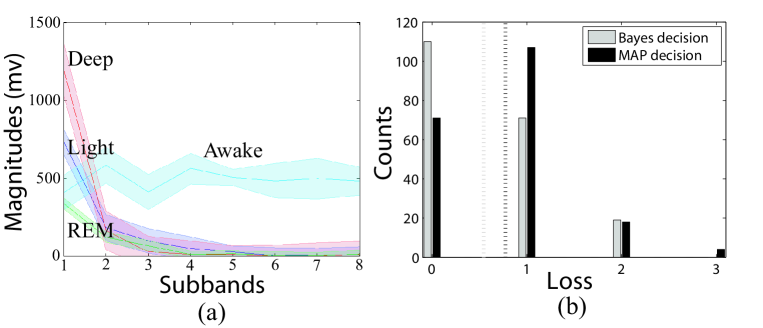
Figure 9: Sleep EEG data analysis. (a) Posterior of the magnitudes in sub-bands. Each plot represents the posterior mean of the magnitudes in the sub-bands with their credible intervals. Different colors represent different sleep stages (cyan: awake, blue: light, red: deep, and green: REM). (b) Histograms of losses of Bayes and MAP decisions for sleep stage monitoring. Vertical dotted lines represent the averaged losses.

We next used these posteriors for making decision rules for automatic sleep scoring. Suppose that $c$ represents one of 4 sleep stages that we need to determine. Our goal is to design an optimal decision rule to minimize the expected loss in terms of the posterior distribution of $c$ given $\mathbf{y}$, which is given by $p(c|\mathbf{y})=\int_{\mathbf{x}}p(c|\mathbf{x})p(\mathbf{x}|\mathbf{y})d\mathbf{x}$. Based on the characteristics of each sleep stage described in [50], we built a simple model for $p(c|\mathbf{x})$ as in the Table II. We denoted awake, light, deep, and rapid-eye-movement (REM) sleep stages as W, L, D, and R for brevity, respectively. The loss function was 3 between $W$ and $D$, 2 between $W$ and $L$; $W$ and $R$; 1 between others.

TABLE II: A rule to design $p(c|\mathbf{x})$. For brevity, awake, light, deep, and REM sleep stages were denoted by W, L, D, and R, respectively.

Conditions of $\mathbf{x}$ $p(\text{W}|\mathbf{x})$ $p(\text{L}|\mathbf{x})$ $p(\text{D}|\mathbf{x})$ $p(\text{R}|\mathbf{x})$ $>35$ Hz takes $>5\%$ of total. 0.8 0.1 0.05 0.05 Total is $<1000$. 0.1 0.2 0.05 0.65 Delta takes $<60\%$ of total. 0.1 0.6 0.2 0.1 Delta takes $\geq 60\%$ of total. 0.05 0.3 0.6 0.05

To evaluate our method, we computed the posterior distributions for 200 non-overlapping sliding windows. The sleep stages that the sleep experts manually annotated were provided for every 30 seconds of the EEG recordings [51]. We used the first 5 second of data in each window to make the problem more challenging. Then we designed an optimal action $a$ given observation $\mathbf{y}$ for each window to minimize the expected loss in terms of the posterior distribution. Fig. 9 (b) illustrates the histograms of the losses for Bayes and MAP decisions for 200 temporal windows. As illustrated, Bayes decision rule incurred smaller losses than MAP decision rule.

Next, we applied our framework to develop a risk-prediction system to predict the survival rates or measure the severity of disease of ICU patients based on physiological measurements. The development of this system is helpful for clinical decision making, standardizing research, comparing the efficacy of medication or the quality of patient care across ICUs. We used real physiological measurements of ICU patients together with their survival outcomes in PhysioNet [48]. Since the outcome $c$ was in binary-class, we designed the optimal action $a$ to take for prediction based on the Bayesian logistic regression that we discussed in the previous subsection. The problem settings were described in the third column of Table I.

Using the ICU data, we computed ROC curves for the Bayes and MAP decisions. Firstly, 10 physiological measurements such as blood urea nitrogen, Galsgow coma score, heart rate, urine output, etc., for 20 subjects were provided with their survival outcomes; For more details of the physiological measurements, refer to PhysioNet [48]. The survival/non-survival outcome of patients $c$ was assigned values 1 or 0. Fig. 10 (a) illustrates the scatter plot of two input variables among 10 variables for 100 subjects as an example: blood urea nitrogen and Galsgow coma score. Fig. 10 (a) shows significant class overlap for these two features (other feature pairs show similar overlap), suggesting a challenging classification task.

Given measurements $\mathbf{y}$ and labels $c$ for the 20 subjects, we computed the posterior $p(\mathbf{x}|\mathbf{y})$ of the unknown parameter $\mathbf{x}$ of the logistic regression model and estimated $\hat{\mathbf{x}}_{\text{MAP}}$ to maximize $p(\mathbf{x}|\mathbf{y})$. Then, physiological measurements for another 100 subjects were provided without their labels. We then computed the ROC curves in the same manner described in the Simulation case.

Fig. 10 (b) illustrates the ROC curves for the Bayes and MAP decision rules obtained using 100 subjects. As shown, the Bayes decision provided us a significantly improved prediction performance over the MAP decision.

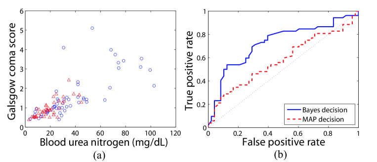
Figure 10: ICU measurements analysis. (a) Scatter plot of two input variables among 10 variables, blood urea nitrogen and Galsgow coma score, for 100 subjects. The blue circle and red plus sign represent survival and non-survival outcomes, respectively. (b) ROC curves for Bayes and MAP decision for predicting survival in ICU.

V Discussion

We have proposed an efficient Bayesian inference method based on finding an optimal map which transforms samples from the prior distribution to samples from the posterior distribution. Although El Moselhy et al. [32] proposed the original optimal maps perspective, their formulation – in terms of minimizing a variance – is in general non-convex and thus computationally intractable. In this setting, we considered an alternative approach, based upon KL divergence minimization, that returns the same optimal solutions. We have also shown consistency results when using finite-dimensional approximations that can be implemented computationally. We have shown that for the class of log-concave priors and likelihoods, this results in a finite-dimensional convex optimization problem. We emphasize that the class of log-concave distributions is quite large and widely used in various applications [1], and that this is the same convexity condition required for Bayesian point (MAP) estimation. As such, we have shown that from the perspective of convexity, we can “get something for nothing” by going from point estimation to fully Bayesian estimation. Through the optimal map, we demonstrated the ability to perform computations, with multi-dimensional parameters, involving the full posterior, including: constructing Bayesian credible regions, attaining the Bayes risk, drawing i.i.d. samples from the posterior, and generating ROC curves.

Other applications outside of Bayesian inference might be able to benefit from this approach. In Section II, we demonstrated a more general result about transforming samples from $P$ to $Q$ whenever $Q$ is log-concave and $P$ can be easily sampled from. Outside the scope of Bayesian inference (where $P$ is the prior and $Q$ is the posterior), this ability may have applications including but are not limited to data compression [6], and message-point feedback information theory [52].

Although we have established convexity of these schemes, further work can be done in developing parallelized optimization algorithms that modern large-scale machine architectures routinely use for Bayesian point estimation. Characterizing the fundamental limits of sample complexity of this approach of Bayesian inference help guide how these architectures may possibly be soundly implemented. Optimizing architectures for hardware optimization, and understanding performance-energy-complexity tradeoffs, will further allow for wider exploration of these methods within the context of emerging applications, such as wearables [53, 54] and the internet-of-things [55].

References

- [1] M. Bagnoli and T. Bergstrom, “Log-concave probability and its applications,” Economic theory, vol. 26, no. 2, pp. 445–469, 2005.
- [2] W. E. Walker, P. Harremoës, J. Rotmans, J. P. van der Sluijs, M. B. van Asselt, P. Janssen, and M. P. Krayer von Krauss, “Defining uncertainty: a conceptual basis for uncertainty management in model-based decision support,” Integrated assessment, vol. 4, no. 1, pp. 5–17, 2003.
- [3] M. H. DeGroot, Optimal statistical decisions. McGraw-Hill, 1970.
- [4] M. Raginsky and T. P. Coleman, “Mutual information and posterior estimates in channels of exponential family type,” in IEEE Inf Theory Workshop, 2009, pp. 399–403.
- [5] M. H. DeGroot, “Uncertainty, information, and sequential experiments,” The Annals of Math Stat, pp. 404–419, 1962.
- [6] T. Cover and J. Thomas, Elements of information theory. Wiley-Interscience, 2006.
- [7] D. Koller and N. Friedman, Probabilistic graphical models: principles and techniques. MIT press, 2009.
- [8] C. J. Quinn, N. Kiyavash, and T. P. Coleman, “Directed information graphs,” IEEE Tran Inf Theory, 2015, to appear.
- [9] R. Kass, L. Tierney, and J. Kadane, “Asymptotics in bayesian computation,” Bayesian statistics, vol. 3, pp. 261–278, 1988.
- [10] Geisser et al., “The validity of posterior expansions based on laplace’s method,” Bayesian and likelihood meth in stat and economet: Essays in honor of George A. Barnard, vol. 7, p. 473, 1990.
- [11] I. J. Good, “Some history of the hierarchical Bayesian methodology,” Trab estadística y invest operat, vol. 31, no. 1, 1980.
- [12] H. Goldstein, Multilevel statistical models. John Wiley & Sons, 2011.
- [13] D. G. Tzikas, C. Likas, and N. P. Galatsanos, “The variational approximation for Bayesian inference,” IEEE Signal Process Mag, vol. 25, no. 6, pp. 131–146, 2008.
- [14] Djuric et al., “Particle filtering,” IEEE Signal Process Mag, vol. 20, no. 5, pp. 19–38, 2003.
- [15] M. S. Arulampalam, S. Maskell, N. Gordon, and T. Clapp, “A tutorial on particle filters for online nonlinear/non-Gaussian Bayesian tracking,” IEEE Tran on Signal Process, vol. 50, no. 2, pp. 174–188, 2002.
- [16] S. G. Walker, P. Damien, P. W. Laud, and A. F. Smith, “Bayesian nonparametric inference for random distributions and related functions,” J Royal Stat Society: Series B (Stat Meth), vol. 61, no. 3, 1999.
- [17] R. M. Neal, “Markov chain sampling methods for dirichlet process mixture models,” J comput and graph stat, vol. 9, no. 2, 2000.
- [18] P. Müller and F. A. Quintana, “Nonparametric Bayesian data analysis,” Stat sci, vol. 19, no. 1, pp. 95–110, 2004.
- [19] Y. W. Teh, M. I. Jordan, M. J. Beal, and D. M. Blei, “Hierarchical Dirichlet processes,” J the american stat assoc, vol. 101, no. 476, 2006.
- [20] C. P. Robert and G. Casella, Monte Carlo statistical methods. Springer, 2004.
- [21] C. Andrieu, N. De Freitas, A. Doucet, and M. I. Jordan, “An introduction to MCMC for machine learning,” Mach learn, vol. 50, no. 1-2, 2003.
- [22] W. K. Hastings, “Monte carlo sampling methods using Markov chains and their applications,” Biometrika, vol. 57, no. 1, pp. 97–109, 1970.
- [23] S. Geman and D. Geman, “Stochastic relaxation, gibbs distributions, and the bayesian restoration of images,” IEEE Trans Pattern Anal Mach Intell, no. 6, pp. 721–741, 1984.
- [24] J. S. Liu, Monte Carlo Strategies in Scientific Computing. Springer, 2008.
- [25] M. I. Jordan, Z. Ghahramani, T. S. Jaakkola, and L. K. Saul, “An introduction to variational methods for graphical models,” Machine learning, vol. 37, no. 2, 1999.
- [26] T. S. Jaakkola, “Tutorial on variational approximation methods,” in In Advanced Mean Field Methods: Theory and Practice. MIT Press, 2000.
- [27] C. M. Bishop, Pattern recognition and machine learning. springer, 2007.
- [28] T. P. Minka, “Expectation propagation for approximate Bayesian inference,” in Uncertainty in artif intell, 2001, pp. 362–369.
- [29] ——, “A family of algorithms for approximate Bayesian inference,” Ph.D. dissertation, Massachusetts Institute of Technology, 2001.
- [30] M. W. Seeger, “Bayesian inference and optimal design for the sparse linear model,” J Mach Learn Research, vol. 9, pp. 759–813, 2008.
- [31] M. I. Jordan, Z. Ghahramani, T. S. Jaakkola, and L. K. Saul, “An introduction to variational methods for graphical models,” Mach learn, vol. 37, no. 2, pp. 183–233, 1999.
- [32] T. El Moselhy and Y. Marzouk, “Bayesian inference with optimal maps,” J Comput Physics, vol. 231, no. 23, pp. 7815–7850, 2012.
- [33] G. Monge, Mémoire sur la théorie des déblais et des remblais. De l’Imprimerie Royale, 1781.
- [34] L. Kantorovich, “On mass transportation,” in Dokl. Akad. Nauk. SSSR, vol. 37, 1942, pp. 227–229.
- [35] C. Villani, Topics in optimal transportation. AMS, 2003.
- [36] M. R. M. D. Kim, S. and T. Coleman, “Efficient Bayesian inference methods via convex optimization and optimal transport,” in IEEE Intern Symp Inf Theory, July 2013, pp. 2259–2263.
- [37] D. Xiu and G. Karniadakis, “The Wiener-Askey polynomial chaos for stochastic differential equations,” SIAM journal on sci comput, vol. 24, no. 2, pp. 619–644, 2003.
- [38] O. G. Ernst, A. Mugler, H. Starkloff, and E. Ullman, “On the convergence of generalized polynomial chaos expansions,” ESAIM: Math Model and Num Analy, vol. 46, pp. 317–339, 2012.
- [39] N. Parikh and S. Boyd, “Proximal algorithms,” Foundations and Trends in Opt, vol. 1, no. 3, pp. 131–231, 2013.
- [40] M. Grant, S. Boyd, and Y. Ye, “Cvx: Matlab software for disciplined convex programming.” [Online]. Available: http://cvxr.com/cvx/
- [41] R. H. Berk, “Consistency and Asymptotic Normality of MLE’s for Exponential Models,” The Annals of Math Stat, vol. 43, no. 1, 1972.
- [42] S. Boyd and L. Vandenberghe, Convex optimization. Cambridge University Press, 2004.
- [43] Y. Li, S.-I. Amari, A. Cichocki, D. W. Ho, and S. Xie, “Underdetermined blind source separation based on sparse representation,” IEEE Tran Signal Process, vol. 54, no. 2, pp. 423–437, 2006.
- [44] A. J. Bell and T. J. Sejnowski, “An information-maximization approach to blind separation and blind deconvolution,” Neural comput, vol. 7, no. 6, pp. 1129–1159, 1995.
- [45] D. P. Wipf and B. D. Rao, “Sparse Bayesian learning for basis selection,” IEEE Tran Signal Process, vol. 52, no. 8, pp. 2153–2164, 2004.
- [46] M. A. Carskadon and A. Rechtschaffen, “Monitoring and staging human sleep,” Principles and practice of sleep medicine, vol. 3, 2000.
- [47] B. Kemp, A. H. Zwinderman, B. Tuk, H. A. Kamphuisen, and J. J. Oberye, “Analysis of a sleep-dependent neuronal feedback loop: the slow-wave microcontinuity of the EEG,” IEEE Tran Biomed Eng, vol. 47, no. 9, pp. 1185–1194, 2000.
- [48] A. L. Goldberger et al., “PhysioBank, PhysioToolkit, and PhysioNet: Components of a new research resource for complex physiologic signals,” Circulation, vol. 101, no. 23, pp. e215–e220, 2000.
- [49] R. McAulay and M. Malpass, “Speech enhancement using a soft-decision noise suppression filter,” IEEE Tran Acoustics, Speech and Signal Process, vol. 28, no. 2, pp. 137–145, 1980.
- [50] M. Ronzhina, O. Janoušek, J. Kolářová, M. Nováková, P. Honzík, and I. Provazník, “Sleep scoring using artificial neural networks,” Sleep Medicine Reviews, vol. 16, no. 3, pp. 251–263, 2012.
- [51] B. Van Sweden, B. Kemp, H. Kamphuisen, and E. Van der Velde, “Alternative electrode placement in (automatic) sleep scoring (Fpz-Cz/Pz-Oz versus C4-A1),” Sleep, vol. 13, no. 3, pp. 279–283, 1990.
- [52] R. Ma and T. Coleman, “Generalizing the posterior matching scheme to higher dimensions via optimal transportation,” in Allerton, 2011.
- [53] D.-H. Kim, N. Lu, R. Ma, Y.-S. Kim, R.-H. Kim, S. Wang, J. Wu, S. M. Won, H. Tao, A. Islam et al., “Epidermal electronics,” Science, vol. 333, no. 6044, pp. 838–843, 2011.
- [54] D. Y. Kang, Y.-S. Kim, G. Ornelas, M. Sinha, K. Naidu, and T. P. Coleman, “Scalable microfabrication procedures for adhesive-integrated flexible and stretchable electronic sensors,” Sensors, vol. 15, no. 9, pp. 23 459–23 476, 2015.
- [55] L. Atzori, A. Iera, and G. Morabito, “The internet of things: A survey,” Computer networks, vol. 54, no. 15, pp. 2787–2805, 2010.