Asynchronous Distributed Optimization
via Randomized Dual Proximal Gradient

Abstract

In this paper we consider distributed optimization problems in which the cost function is separable, i.e., a sum of possibly non-smooth functions all sharing a common variable, and can be split into a strongly convex term and a convex one. The second term is typically used to encode constraints or to regularize the solution. We propose a class of distributed optimization algorithms based on proximal gradient methods applied to the dual problem. We show that, by choosing suitable primal variable copies, the dual problem is itself separable when written in terms of conjugate functions, and the dual variables can be stacked into non-overlapping blocks associated to the computing nodes. We first show that a weighted proximal gradient on the dual function leads to a synchronous distributed algorithm with local dual proximal gradient updates at each node. Then, as main paper contribution, we develop asynchronous versions of the algorithm in which the node updates are triggered by local timers without any global iteration counter. The algorithms are shown to be proper randomized block-coordinate proximal gradient updates on the dual function.

I Introduction

Several estimation, learning, decision and control problems arising in cyber-physical networks involve the distributed solution of a constrained optimization problem. Typically, computing processors have only a partial knowledge of the problem (e.g. a portion of the cost function or a subset of the constraints) and need to cooperate in order to compute a global solution of the whole problem. A key challenge when designing distributed optimization algorithms in peer-to-peer networks is that the communication among the nodes is time-varying and possibly asynchronous.

Early references on distributed optimization algorithms involved primal and dual subgradient methods and Alternating Direction Method of Multipliers (ADMM), designed for synchronous communication protocols over fixed graphs. More recently time-varying versions of these algorithmic ideas have been proposed to cope with more realistic peer-to-peer network scenarios. A Newton-Raphson consensus strategy is proposed in [1] to solve unconstrained, convex optimization problems under asynchronous, symmetric gossip communications. In [2] a primal, synchronous algorithm, called EXTRA, is proposed to solve smooth, unconstrained optimization problems. In [3] the authors propose accelerated distributed gradient methods for unconstrained optimization problems over symmetric, time-varying networks connected on average. In order to deal with time-varying and directed graph topologies, in [4] a push-sum algorithm for average consensus is combined with a primal subgradient method in order to solve unconstrained convex optimization problems. Paper [5] extends this algorithm to online distributed optimization over time-varying, directed networks. In [6] a novel class of continuous-time, gradient-based distributed algorithms is proposed both for fixed and time-varying graphs and conditions for exponential convergence are provided. A distributed (primal) proximal-gradient method is proposed in [7] to solve (over time-varying, balanced communication graphs) optimization problems with a separable cost function including local differentiable components and a common non-differentiable term. In [8] experiments of a dual averaging algorithm are run for separable problems with a common constraint on time-varying and directed networks.

For general constrained convex optimization problems, in [9] the authors propose a distributed random projection algorithm, that can be used by multiple agents connected over a (balanced) time-varying network. In [10] the author proposes (primal) randomized block-coordinate descent methods for minimizing multi-agent convex optimization problems with linearly coupled constraints over networks. In [11] an asynchronous ADMM-based distributed method is proposed for a separable, constrained optimization problem. The algorithm is shown to converge at the rate $O(1/t)$ (being $t$ the iteration counter). In [12] the ADMM approach is proposed for a more general framework, thus yielding a continuum of algorithms ranging from a fully centralized to a fully distributed. In [13] a method, called ADMM+, is proposed to solve separable, convex optimization problems with a cost function written as the sum of a smooth and a non-smooth term.

Successive block-coordinate updates are proposed in [14, 15] to solve separable optimization problems in a parallel big-data setting. Another class of algorithms exploits the exchange of active constraints among the network nodes to solve constrained optimization problems [16]. This idea has been combined with dual decomposition and cutting-plane methods to solve robust convex optimization problems via polyhedral approximations [17]. These algorithms work under asynchronous, direct and unreliable communication.

The contribution of the paper is twofold. First, for a fixed graph topology, we develop a distributed optimization algorithm (based on a centralized dual proximal gradient idea introduced in [18]) to minimize a separable strongly convex cost function. The proposed distributed algorithm is based on a proper choice of primal constraints (suitably separating the graph-induced and node-local constraints), that gives rise to a dual problem with a separable structure when expressed in terms of local conjugate functions. Thus, a proximal gradient applied to such a dual problem turns out to be a distributed algorithm where each node updates: (i) its primal variable through a local minimization and (ii) its dual variables through a suitable local proximal gradient step. The algorithm inherits the convergence properties of the centralized one and thus exhibits an $O(1/t)$ (being $t$ the iteration counter) rate of convergence in objective value. We point out that the algorithm can be accelerated through a Nesterov’s scheme, [19], thus obtaining an $O(1/t^{2})$ convergence rate.

Second, as main contribution, we propose an asynchronous algorithm for a symmetric event-triggered communication protocol. In this communication set-up, a node is in idle mode until its local timer triggers. When in idle, it continuously collects messages from neighboring nodes that are awake and, if needed, updates a primal variable. When the local timer triggers, it updates local primal and dual variables and broadcasts them to neighboring nodes. Under mild assumptions on the local timers, the whole algorithm results into a uniform random choice of one active node per iteration. Using this property and showing that the dual variables can be stacked into separate blocks, we are able to prove that the distributed algorithm corresponds to a block-coordinate proximal gradient, as the one proposed in [20], performed on the dual problem. Specifically, we are able to show that the dual variables handled by a single node represent a single variable-block, and the local update at each triggered node turns out to be a block-coordinate proximal gradient step (in which each node has its own local step-size). The result is that the algorithm inherits the convergence properties of the block-coordinate proximal gradient in [20].

An important property of the distributed algorithm is that it can solve fairly general optimization problems including both composite cost functions and local constraints. A key distinctive feature of the algorithm analysis is the combination of duality theory, coordinate-descent methods, and properties of the proximal operator when applied to conjugate functions.

To summarize, our algorithms compare to the literature in the following way. Works in [1, 3, 4, 5, 6] do not handle constrained optimization and use different methodologies. In [7, 9, 10] primal approaches are used. Also, local constraints and regularization terms cannot be handled simultaneously. In [7] a proximal operator is used, but only to handle a common, non-smooth cost function (known by all agents) directly on the primal problem. The algorithm in [10] uses a coordinate-descent idea similar to the one we use in this paper, but it works directly on the primal problem, does not handle local constraints and does not make use of proximal operators. In this paper we propose a flexible dual approach to take into account both local constraints and regularization terms. The problem set-up in [11, 12, 13] is similar to the one considered in this paper. Differently from our approach, which is a dual method, ADMM-based algorithms are proposed in those references. This difference results in different algorithms as well as different requirements on the cost functions. Moreover, compared to these algorithms we are able to use constant, local step-sizes (which can be locally computed at the beginning of the iterations) so that the algorithm can be run asynchronously and without any coordination step. On this regard, we propose an algorithmic formulation of the asynchronous protocol that explicitly relies on local timers and does not need any global iteration counter in the update laws.

The paper is organized as follows. In Section II we set-up the optimization problem, while in Section III we derive an equivalent dual problem amenable for distributed computation. The distributed algorithms are introduced in Section IV and analyzed in Section V. Finally, in Section VI we highlight the flexibility of the proposed algorithms by showing important optimization scenarios that can be addressed, and corroborate the discussion with numerical computations.

Notation

Given a closed, nonempty convex set $X$, the indicator function of $X$ is defined as $I_{X}(x)=0$ if $x\in X$ and $I_{X}(x)=+\infty$ otherwise. Let $\varphi\,:\,^{d}\to\cup\{+\infty\}$, its conjugate function $\varphi^{*}\,:\,^{d}\to$ is defined as $\varphi^{*}(y):=\sup_{x}\big{\{}y^{\top}x-\varphi(x)\big{\}}$. Let $\varphi\,:\,^{d}\to\cup\{+\infty\}$ be a closed, proper, convex function and $\alpha$ a positive scalar, the proximal operator $\mathbf{prox}_{\alpha\varphi}\,:\,^{d}\to^{d}$ is defined by $\mathbf{prox}_{\alpha\varphi}(v):=\mathop{\rm argmin}_{x}\big{\{}\varphi(x)+\frac{1}{2\alpha}\|x-v\|^{2}\big{\}}$. We also introduce a generalized version of the proximal operator. Given a positive definite matrix $W\in^{d\times d}$, we define

$$\mathbf{prox}_{W,\varphi}(v):=\mathop{\rm argmin}_{x}\Big{\{}\varphi(x)+\frac{1}{2}\big{\|}x-v\big{\|}^{2}_{W^{-1}}\Big{\}}.$$

II Problem set-up and network structure

We consider the following optimization problem

$$\min_{x}\sum_{i=1}^{n}\Big{(}f_{i}(x)+g_{i}(x)\Big{)},$$ (1)

where $f_{i}:^{d}\to\cup\{+\infty\}$ are proper, closed and strongly convex extended real-valued functions with strong convexity parameter $\sigma_{i}>0$ and $g_{i}:^{d}\to\cup\{+\infty\}$ are proper, closed and convex extended real-valued functions.

Note that the split of $f_{i}$ and $g_{i}$ may be non-unique and depend on the problem structure. Intuitively, on $f_{i}$ an easy minimization step can be performed (e.g., by division free operations, [21]), while $g_{i}$ has an easy expression of its proximal operator.

Remark II.1 (Min-max problems).

Our setup does not require $f_{i}$ to be differentiable, thus one can also consider each strongly convex function $f_{i}$ given by $f_{i}(x):=\max_{j\in\{1,\ldots,m_{i}\}}f_{ij}(x)$, $m_{i}\in{\mathbb{N}}$, where $\{f_{ij}(x)\mid j\in\{1,\ldots,m_{i}\}\}$ is a nonempty collection of strongly convex functions. $\square$

Since we will work on the dual of problem (1), we introduce the next standard assumption which guarantees that the dual is feasible and equivalent to the primal (strong duality).

Assumption II.2 (Constraint qualification).

The intersection of the relative interior of $\mathop{\bf dom}\,\sum_{i=1}^{n}f_{i}$ and the relative interior of $\mathop{\bf dom}\,\sum_{i=1}^{n}g_{i}$ is non-empty. $\square$

We want this optimization problem to be solved in a distributed way by a network of peer processors without a central coordinator. Each processor has a local memory, a local computation capability and can exchange information with neighboring nodes. We assume that the communication can occur among nodes that are neighbors in a given fixed, undirected and connected graph $\mathcal{G}=(\{1,\ldots,n\},\mathcal{E})$, where $\mathcal{E}\subseteq\{1,\ldots,n\}\times\{1,\ldots,n\}$ is the set of edges. That is, the edge $(i,j)$ models the fact that node $i$ and $j$ can exchange information. We denote by $\mathcal{N}_{i}$ the set of neighbors of node $i$ in the fixed graph $\mathcal{G}$, i.e., $\mathcal{N}_{i}:=\left\{j\in\{1,\ldots,n\}\mid(i,j)\in\mathcal{E}\right\}$, and by $|\mathcal{N}_{i}|$ its cardinality.

In Section IV we will propose distributed algorithms for three communication protocols. Namely, we will consider a synchronous protocol (in which neighboring nodes in the graph communicate according to a common clock), and two asynchronous ones, respectively node-based and edge-based (in which nodes become active according to local timers).

To exploit the sparsity of the graph we introduce copies of $x$ and their coherence (consensus) constraint, so that the optimization problem (1) can be equivalently rewritten as

$$\begin{split}\min_{x_{1},\ldots,x_{n}}&\;\sum_{i=1}^{n}\Big{(}f_{i}(x_{i})+g_{i}(x_{i})\Big{)}\\ \text{subj. to}&\;x_{i}=x_{j}\hskip 11.38092pt\forall\,(i,j)\in\mathcal{E}\end{split}$$ (2)

with $x_{i}\in^{d}$ for all $i\in\{1,\ldots,n\}$. The connectedness of $\mathcal{G}$ guarantees the equivalence.

Since we propose distributed dual algorithms, next we derive the dual problem and characterize its properties.

III Dual problem derivation

We derive the dual version of the problem that will allow us to design our distributed dual proximal gradient algorithms. To obtain the desired separable structure of the dual problem, we set-up an equivalent formulation of problem (2) by adding new variables $z_{i}$, $i\in\{1,\ldots,n\}$, i.e.,

$$\begin{split}\min_{\stackrel{{\scriptstyle x_{1},\ldots,x_{n}}}{{z_{1},\ldots,z_{n}}}}&\;\sum_{i=1}^{n}\Big{(}f_{i}(x_{i})+g_{i}(z_{i})\Big{)}\\ \text{subj. to}&\;x_{i}=x_{j}\hskip 11.38092pt\forall\,(i,j)\in\mathcal{E}\\ &\;x_{i}=z_{i}\hskip 14.22636pt\forall\,i\in\{1,\ldots,n\}.\end{split}$$ (3)

Let ${\bf x}=[x_{1}^{\top}\,\ldots\,x_{n}^{\top}]^{\top}$ and ${\bf z}=[z_{1}^{\top}\,\ldots\,z_{n}^{\top}]^{\top}$, the Lagrangian of primal problem (3) is given by

$$L(\mathbf{x},\mathbf{z},\Lambda,\mu) =\sum_{i=1}^{n}\bigg{(}f_{i}(x_{i})+g_{i}(z_{i})$$

$$\hskip 19.91684pt+\sum_{j\in\mathcal{N}_{i}}\left(\lambda_{i}^{j}\right)^{\top}(x_{i}-x_{j})+\mu_{i}^{\top}(x_{i}-z_{i})\bigg{)}$$

$$=\sum_{i=1}^{n}\!\bigg{(}f_{i}(x_{i})+\!\sum_{j\in\mathcal{N}_{i}}\!\Big{(}\lambda_{i}^{j}\Big{)}^{\top}\!(x_{i}-x_{j})+\mu_{i}^{\top}x_{i}$$

$$\hskip 28.45274pt+g_{i}(z_{i})-\mu_{i}^{\top}z_{i}\bigg{)},$$

where $\Lambda$ and $\mu$ are respectively the vectors of the Lagrange multipliers $\lambda_{i}^{j}$, $(i,j)\in\mathcal{E}$, and $\mu_{i}$, $i\in\{1,\ldots,n\}$, and in the last line we have separated the terms in $\mathbf{x}$ and $\mathbf{z}$. Since $\mathcal{G}$ is undirected, the Lagrangian can be rearranged as

$$L(\mathbf{x},\mathbf{z},\Lambda,\mu) =\sum_{i=1}^{n}\bigg{(}f_{i}(x_{i})+x_{i}^{\top}\Big{(}\sum_{j\in\mathcal{N}_{i}}(\lambda_{i}^{j}-\lambda_{j}^{i})+\mu_{i}\Big{)}$$

$$\hskip 34.14322pt+g_{i}(z_{i})-z_{i}^{\top}\mu_{i}\bigg{)}.$$

The dual function is

$$q(\Lambda,\mu) :=\min_{\mathbf{x},\mathbf{z}}L(\mathbf{x},\mathbf{z},\Lambda,\mu)$$

$$=\min_{\mathbf{x}}\sum_{i=1}^{n}\bigg{(}f_{i}(x_{i})+x_{i}^{\top}\bigg{(}\sum_{j\in\mathcal{N}_{i}}(\lambda_{i}^{j}-\lambda_{j}^{i})+\mu_{i}\bigg{)}\bigg{)}$$

$$\hskip 28.45274pt+\min_{\mathbf{z}}\sum_{i=1}^{n}\Big{(}g_{i}(z_{i})-z_{i}^{\top}\mu_{i}\Big{)}$$

$$=\sum_{i=1}^{n}\min_{x_{i}}\bigg{(}f_{i}(x_{i})+x_{i}^{\top}\Big{(}\sum_{j\in\mathcal{N}_{i}}(\lambda_{i}^{j}-\lambda_{j}^{i})+\mu_{i}\Big{)}\bigg{)}$$

$$\hskip 28.45274pt+\sum_{i=1}^{n}\min_{z_{i}}\Big{(}g_{i}(z_{i})-z_{i}^{\top}\mu_{i}\Big{)},$$

where we have used the separability of the Lagrangian with respect to each $x_{i}$ and each $z_{i}$. Then, by using the definition of conjugate function (given in the Notation paragraph), the dual function can be expressed as

$$q(\Lambda,\mu) =\sum_{i=1}^{n}\Bigg{(}\!\!-\!f_{i}^{*}\bigg{(}\!-\!\sum_{j\in\mathcal{N}_{i}}(\lambda_{i}^{j}-\lambda_{j}^{i})-\mu_{i}\bigg{)}\!-g_{i}^{*}(\mu_{i})\Bigg{)}.$$

The dual problem of (3) consists of maximizing the dual function with respect to dual variables $\Lambda$ and $\mu$, i.e.

$$\!\!\max_{\Lambda,\mu} \;\sum_{i=1}^{n}\bigg{(}\!\!-\!f_{i}^{*}\bigg{(}\!-\!\sum_{j\in\mathcal{N}_{i}}(\lambda_{i}^{j}-\lambda_{j}^{i})-\mu_{i}\bigg{)}\!-g_{i}^{*}(\mu_{i})\bigg{)}.$$ (4)

By Assumption II.2 the dual problem (4) is feasible and strong duality holds, so that (4) can be equivalently solved to get a solution of (3).

In order to have a more compact notation for problem (4), we stack the dual variables as $y=[y_{1}^{\top}\;\ldots\;y_{n}^{\top}]^{\top}$, where

$$y_{i}=\begin{bmatrix}\Lambda_{i}\\ \mu_{i}\end{bmatrix}\in^{d|\mathcal{N}_{i}|+d}$$ (5)

with $\Lambda_{i}\in^{d|\mathcal{N}_{i}|}$ a vector whose block-component associated to neighbor $j$ is $\lambda_{i}^{j}\in^{d}$. Thus, changing sign to the cost function, dual problem (4) can be restated as

$$\min_{y} \;\Gamma(y)=F^{*}(y)+G^{*}(y),$$ (6)

where

$$F^{*}\!(y)\!:=\!\sum_{i=1}^{n}f_{i}^{*}\Big{(}\!\!-\!\!\sum_{j\in\mathcal{N}_{i}}(\lambda_{i}^{j}-\lambda_{j}^{i})-\mu_{i}\Big{)},G^{*}\!(y)\!:=\!\sum_{i=1}^{n}g_{i}^{*}\big{(}\mu_{i}\big{)}.$$

IV Distributed dual proximal algorithms

In this section we derive the distributed optimization algorithms based on dual proximal gradient methods.

IV-A Synchronous Distributed Dual Proximal Gradient

We begin by deriving a synchronous algorithm on a fixed graph. We assume that all the nodes share a common clock. At each time instant $t\in{\mathbb{N}}$, every node communicates with its neighbors in the graph $\mathcal{G}=(\{1,\ldots,n\},\mathcal{E})$ (defined in Section II) and updates its local variables.

First, we provide an informal description of the distributed optimization algorithm. Each node $i\in\{1,\ldots,n\}$ stores a set of local dual variables $\lambda_{i}^{j}$, $j\in\mathcal{N}_{i}$, and $\mu_{i}$, updated through a local proximal gradient step, and a primal variable $x_{i}^{\star}$, updated through a local minimization. Each node uses a properly chosen, local step-size $\alpha_{i}$ for the proximal gradient step. Then, the updated primal and dual values are exchanged with the neighboring nodes. The local dual variables at node $i$ are initialized as $\lambda_{i0}^{j}$, $j\in\mathcal{N}_{i}$, and $\mu_{i0}$. A pseudo-code of the local update at each node of the distributed algorithm is given in Algorithm 1.

Processor states: $x_{i}^{\star}$, $\lambda_{i}^{j}$ for all $j\in\mathcal{N}_{i}$ and $\mu_{i}$

Initialization: $\lambda_{i}^{j}(0)=\lambda_{i0}^{j}$ for all $j\in\mathcal{N}_{i}$, $\mu_{i}(0)=\mu_{i0}$

    $\!\!x_{i}^{\star}(0)=\mathop{\rm argmin}_{x_{i}}\left\{\!x_{i}^{\top}\!\left(\!\sum_{j\in\mathcal{N}_{i}}\!\left(\!\lambda_{i0}^{j}-\lambda_{j0}^{i}\!\right)\!+\!\mu_{i0}\!\right)\!+\!f_{i}(x_{i})\!\right\}\vskip 6.0pt plus 2.0pt minus 2.0pt$

Evolution:

 for: $t=1,2,\ldots$ do

   receive $x_{j}^{\star}(t-1)$ for each $j\in\mathcal{N}_{i}$, update

$$\!\!\!\lambda_{i}^{j}(t) =\lambda_{i}^{j}(t-1)+\alpha_{i}\left[x_{i}^{\star}(t-1)-x_{j}^{\star}(t-1)\right]$$

   and update

$$\tilde{\mu}_{i}=\mu_{i}(t-1)+\alpha_{i}\;x_{i}^{\star}(t-1)$$

$$\mu_{i}(t)=\tilde{\mu}_{i}-\alpha_{i}\;\mathbf{prox}_{\frac{1}{\alpha_{i}}g_{i}}\left(\frac{\tilde{\mu}_{i}}{\alpha_{i}}\right)$$

   receive $\lambda_{j}^{i}(t)$ for each $j\in\mathcal{N}_{i}$ and compute

$$\!\!\!x_{i}^{\star}(t)=\mathop{\rm argmin}_{x_{i}}\bigg{\{}\!x_{i}^{\top}\!\bigg{(}\sum_{j\in\mathcal{N}_{i}}\!\Big{(}\!\lambda_{i}^{j}(t)-\lambda_{j}^{i}(t)\!\Big{)}\!+\!\mu_{i}(t)\!\bigg{)}\!+\!f_{i}(x_{i})\!\bigg{\}}$$

Algorithm 1 Distributed Dual Proximal Gradient

Remark IV.1.

In order to start the algorithm, a preliminary communication step is needed in which each node $i$ receives from each neighbor $j$ its $\lambda_{j0}^{i}$ (to compute $x_{i}^{\star}(0)$) and the convexity parameter $\sigma_{j}$ of $f_{j}$ (to set $\alpha_{i}$, as it will be clear from the analysis in Section V-B). This step can be avoided if the nodes agree to set $\lambda_{i0}^{j}=0$ and know a bound for $\alpha_{i}$. Also, it is worth noting that, differently from other algorithms, in general $\lambda_{i}^{j}(t)\neq-\lambda_{j}^{i}(t)$.   $\square$

We point out once more that to run the Distributed Dual Proximal Gradient algorithm the nodes need to have a common clock. Also, it is worth noting that, as it will be clear from the analysis in Section V-B, to set the local step-size each node needs to know the number of nodes, $n$, in the network. In the next sections we present two asynchronous distributed algorithms which overcome these limitations.

IV-B Asynchronous Distributed Dual Proximal Gradient

Next, we propose a node-based asynchronous algorithm. We consider an asynchronous protocol where each node has its own concept of time defined by a local timer, which randomly and independently of the other nodes triggers when to awake itself. Between two triggering events the node is in an idle mode, i.e., it continuously receives messages from neighboring nodes and, if needed, runs some auxiliary computation. When a trigger occurs, it switches into an awake mode in which it updates its local (primal and dual) variables and transmits the updated information to its neighbors.

Formally, the triggering process is modeled by means of a local clock $\tau_{i}\in_{\geq 0}$ and a randomly generated waiting time $T_{i}$. As long as $\tau_{i}<T_{i}$ the node is in idle mode. When $\tau_{i}=T_{i}$ the node switches to the awake mode and, after running the local computation, resets $\tau_{i}=0$ and draws a new realization of the random variable $T_{i}$. We make the following assumption on the local waiting times $T_{i}$.

Assumption IV.2 (Exponential i.i.d. local timers).

The waiting times between consecutive triggering events are i.i.d. random variables with same exponential distribution.  $\square$

When a node $i$ wakes up, it updates its local dual variables $\lambda_{i}^{j}$, $j\in\mathcal{N}_{i}$ and $\mu_{i}$ by a local proximal gradient step, and its primal variable $x_{i}^{\star}$ through a local minimization. The local step-size of the proximal gradient step for node $i$ is denoted by $\alpha_{i}$. In order to highlight the difference between updated and old variables at node $i$ during the “awake” phase, we denote the updated ones as ${\lambda_{i}^{j}}^{+}$ and ${\mu_{i}}^{+}$ respectively. When a node $i$ is in idle it receives messages from awake neighbors. If a dual variable $\lambda_{j}^{i}$ is received it computes an updated value of ${x_{i}^{\star}}$ and broadcasts it to its neighbors. It is worth noting that, being the algorithm asynchronous, there is no common clock as in the synchronous version.

Processor states: $x_{i}^{\star}$, $\lambda_{i}^{j}$ for all $j\in\mathcal{N}_{i}$ and $\mu_{i}$

Initialization: $\lambda_{i}^{j}=\lambda_{i0}^{j}$ for all $j\in\mathcal{N}_{i}$, $\mu_{i}=\mu_{i0}$ and

     $x_{i}^{\star}={\displaystyle\mathop{\rm argmin}_{x_{i}}}\Big{\{}\!x_{i}^{\top}\!\Big{(}\!\sum_{j\in\mathcal{N}_{i}}\!\Big{(}\!\lambda_{i0}^{j}-\lambda_{j0}^{i}\!\Big{)}\!+\!\mu_{i0}\!\Big{)}\!+\!f_{i}(x_{i})\!\Big{\}}$

     set $\tau_{i}=0$ and get a realization $T_{i}$

Evolution:

IDLE:

   while: $\tau_{i}<T_{i}$ do:

     receive $x_{j}^{\star}$ and/or $\lambda_{j}^{i}$ from each $j\in\mathcal{N}_{i}$.

     if: $\lambda_{j}^{i}$ is received then: compute and broadcast

$$x_{i}^{\star}=\mathop{\rm argmin}_{x_{i}}\bigg{\{}x_{i}^{\top}\bigg{(}\sum_{k\in\mathcal{N}_{i}}\Big{(}\lambda_{i}^{k}-\lambda_{k}^{i}\Big{)}+\mu_{i}\bigg{)}+f_{i}(x_{i})\bigg{\}}$$

   go to AWAKE.

AWAKE:

   update and broadcast ${\lambda_{i}^{j}}^{+}\!\!=\!\lambda_{i}^{j}+\alpha_{i}\big{(}x_{i}^{\star}-x_{j}^{\star}\big{)},\forall\,j\in\mathcal{N}_{i}$

   update

$$\tilde{\mu}_{i}=\mu_{i}+\alpha_{i}\;x_{i}^{\star}$$

$$\mu_{i}^{+}=\tilde{\mu}_{i}-\alpha_{i}\;\mathbf{prox}_{\frac{1}{\alpha_{i}}g_{i}}\left(\frac{\tilde{\mu}_{i}}{\alpha_{i}}\right)$$

   compute and broadcast

$$x_{i}^{\star}=\mathop{\rm argmin}_{x_{i}}\bigg{\{}x_{i}^{\top}\bigg{(}\sum_{j\in\mathcal{N}_{i}}\Big{(}{\lambda_{i}^{j}}^{+}-\lambda_{j}^{i}\Big{)}+\mu^{+}_{i}\bigg{)}+f_{i}(x_{i})\bigg{\}}$$

   set $\tau_{i}=0$, get a new realization $T_{i}$ and go to IDLE.

Algorithm 2 Asynchronous Distributed Dual Proximal Gradient

IV-C Edge-based asynchronous algorithm

In this section we present a variant of the Asynchronous Distributed Dual Proximal Gradient in which an edge becomes active uniformly at random, rather than a node. In other words, we assume that timers are associated to edges, rather than to nodes, that is a waiting time $T_{ij}$ is extracted for edge $(i,j)$.

The processor states and their initialization stay the same except for the timers. Notice that here we are assuming that nodes $i$ and $j$ have a common waiting time $T_{ij}$ and, consistently, a local timer $\tau_{ij}$. Each waiting time $T_{ij}$ satisfies Assumption IV.2.

In Algorithm 3 we report (only) the evolution for this modified scenario. In this edge-based algorithm the dual variable $\mu_{i}$ (associated to the constraint $x_{i}=z_{i}$) cannot be updated every time an edge $(i,j)$, $j\in\mathcal{N}_{i}$, becomes active (otherwise it would be updated more often than the variables $\lambda_{i}^{j}$, $j\in\mathcal{N}_{i}$). Thus, we identify one special neighbor $j_{\mu_{i}}\in\mathcal{N}_{i}$ and update $\mu_{i}$ only when the edge $(i,j_{\mu_{i}})$ is active.

IDLE: while $\tau_{ij}<T_{ij}$ do: nothing

   go to AWAKE.

AWAKE:

   send $x_{i}^{\star}$ to $j$ and receive $x_{j}^{\star}$ from $j$

   update and send to $j$, ${\lambda_{i}^{j}}^{+}=\lambda_{i}^{j}+\alpha_{i}\big{(}x_{i}^{\star}-x_{j}^{\star}\big{)}$

   if: $j=j_{\mu_{i}}$ then: update $\mu_{i}^{+}=\mathbf{prox}_{\alpha_{i}g_{i}^{*}}\big{(}\mu_{i}+\alpha_{i}\;x_{i}^{\star}\big{)}$

   compute

$$x_{i}^{\star}=\mathop{\rm argmin}_{x_{i}}\bigg{\{}x_{i}^{\top}\bigg{(}\sum_{j\in\mathcal{N}_{i}}\Big{(}{\lambda_{i}^{j}}^{+}-\lambda_{j}^{i}\Big{)}+\mu^{+}_{i}\bigg{)}+f_{i}(x_{i})\bigg{\}}$$

   set $\tau_{ij}=0$, deal on a new realization $T_{ij}$ and go to IDLE.

Algorithm 3 Edge-Based Formulation of Algorithm 2 (evolution)

V Analysis of the distributed algorithms

To start the analysis we first introduce an extended version of (centralized) proximal gradient methods.

V-A Weighted Proximal Gradient Methods

Consider the following optimization problem

$$\min_{y\in^{N}}\>\>\Gamma(y):=\Phi(y)+\Psi(y),$$ (7)

where $\Phi:^{N}\to$ and $\Psi:^{N}\to\cup\{+\infty\}$ are convex functions.

We decompose the decision variable as $y=[y_{1}^{\top}\;\ldots\;y_{n}^{\top}]^{\top}$ and, consistently, we decompose the space ^N into $n$ subspaces as follows. Let $U\in^{N\times N}$ be a column permutation of the $N\times N$ identity matrix and, further, let $U=[U_{1}\;U_{2}\;\ldots\;U_{n}]$ be a decomposition of $U$ into $n$ submatrices, with $U_{i}\in^{N\times N_{i}}$ and $\sum_{i}N_{i}=N$. Thus, any vector $y\in^{N}$ can be uniquely written as $y=\sum_{i}U_{i}y_{i}$ and, viceversa, $y_{i}=U_{i}^{\top}y$.

We let problem (7) satisfy the following assumptions.

Assumption V.1 (Block Lipschitz continuity of $\nabla\Phi$).

The gradient of $\Phi$ is block coordinate-wise Lipschitz continuous with positive constants $L_{1},\ldots,L_{n}$. That is, for all $y\in^{N}$ and $s_{i}\in^{N_{i}}$ it holds

$$\|\nabla_{i}\Phi(y+U_{i}s_{i})-\nabla_{i}\Phi(y)\|\leq L_{i}\|s_{i}\|,$$

where $\nabla_{i}\Phi(y)$ is the $i$-th block component of $\nabla\Phi(y)$.  $\square$

Assumption V.2 (Separability of $\Psi$).

The function $\Psi$ is block-separable, i.e., it can be decomposed as $\Psi(y)=\sum_{i=1}^{n}\psi_{i}(y_{i})$, with each $\psi_{i}:^{N_{i}}\to\!\cup\!\{+\infty\}$ a proper, closed convex extended real-valued function.  $\square$

Assumption V.3 (Feasibility).

The set of minimizers of problem (7) is non-empty.  $\square$

V-A1 Deterministic descent

We first show how the standard proximal gradient algorithm can be generalized by using a weighted proximal operator.

Following the same line of proof as in [18], we can prove that a generalized proximal gradient iteration, given by

$$y(t+1)=\mathbf{prox}_{W,\Psi}\Big{(}y(t)-W\nabla\Phi\big{(}y(t)\big{)}\Big{)}$$ (8)

$$\hskip 8.5359pt=\mathop{\rm argmin}_{y}\bigg{\{}\!\Psi(y)\!+\!\frac{1}{2}\Big{\|}y\!-\!\Big{(}y(t)-W\nabla\Phi\big{(}y(t)\big{)}\Big{)}\Big{\|}_{W^{-1}}^{2}\!\bigg{\}},$$

converges in objective value to the optimal solution of (7) with rate $O(1/t)$.

In order to extend the proof of [18, Theorem 3.1] we need to use a generalized version of [18, Lemma 2.1]. To this end we can use a result by Nesterov, given in [22], which is recalled in the following lemma for completeness.

Lemma V.4 (Generalized Descent Lemma).

Let Assumption V.1 hold, then for all $s\in^{N}$

$$\Phi(y+s)\leq\Phi(y)+s^{\top}\nabla\Phi(y)+\frac{1}{2}\big{\|}\,s\,\big{\|}_{W^{-1}}^{2},$$

where $W:=\operatorname{diag}(w_{1},\ldots,w_{n})$ satisfies $w_{i}\leq\frac{1}{nL_{i}}$ for all $i\in\{1,\ldots,n\}$. $\square$

Tighter conditions than the one given above can be found in [14] and in [23].

Theorem V.5.

Let Assumption V.1 and V.3 hold and let $\{y(t)\}$ be the sequence generated by iteration (8) applied to problem (7). Then for any $t\geq 1$

$$\Gamma(y(t))-\Gamma(y^{\star})\leq\frac{\big{\|}y_{0}-y^{\star}\big{\|}^{2}_{W^{-1}}}{2t},$$

where $W:=\operatorname{diag}(w_{1},\ldots,w_{n})$ with $w_{i}\leq\frac{1}{nL_{i}}$, $y_{0}$ is the initial condition and $y^{\star}$ is any minimizer of problem (7).

Proof.

The theorem is proven by following the same arguments as in [18, Theorem 3.1], but using Lemma V.4 in place of [18, Lemma 2.1]. ∎

V-A2 Randomized block coordinate descent

Next, we present a randomized version of the weighted proximal gradient, proposed in [20, Algorithm $2$] as Uniform Coordinate Descent for Composite functions (UCDC) algorithm.

Initialization: $y(0)=y_{0}$

for: $t=0,1,2,\ldots$ do

 choose $i_{t}\in\{1,\ldots,n\}$ with probability $\frac{1}{n}$

 compute

$$T^{(i_{t})}\big{(}y(t)\big{)}=\mathop{\rm argmin}_{s\in^{N_{i_{t}}}}\Big{\{}V_{i_{t}}(y(t),s)\Big{\}}$$ (9a)

   where

$$V_{i_{t}}(y,s)\!:=\!\nabla_{i_{t}}\Phi(y)^{\top}s\!+\!\frac{L_{i_{t}}}{2}\|s\|^{2}\!+\!\psi_{i_{t}}(y_{i_{t}}\!+\!s)$$ (9b)

 update

$$y(t+1)=y(t)+U_{i_{t}}T^{(i_{t})}\big{(}y(t)\big{)}.$$ (10)

Algorithm 4 UCDC

The convergence result for UCDC is given in [20, Theorem $5$], here reported for completeness.

Theorem V.6 ([20, Theorem $5$]).

Let Assumptions V.1, V.2 and V.3 hold. Let $\Gamma^{\star}$ denote the optimal cost of problem (7). Then, for any $\varepsilon\in\Big{(}0,\Gamma(y_{0})-\Gamma^{\star}\Big{)}$, there exists $\bar{t}(\varepsilon,\rho)>0$ such that if $y(t)$ is the random sequence generated by UCDC (Algorithm 4) applied to problem (7), then for all $t\geq\bar{t}$ it holds that

$$\Pr\Big{(}\Gamma(y(t))-\Gamma^{\star}\leq\varepsilon\Big{)}\geq 1-\rho,$$

where $y_{0}\in^{N}$ is the initial condition and $\rho\in(0,1)$ is the target confidence.  $\square$

V-B Analysis of the synchronous algorithm

We start this section by recalling some useful properties of conjugate functions that will be useful for the convergence analysis of the proposed distributed algorithms.

Lemma V.7 ([24, 25]).

Let $\varphi$ be a closed, strictly convex function and $\varphi^{*}$ its conjugate function. Then

$$\nabla\varphi^{*}(y)\!=\!\mathop{\rm argmax}_{x}\left\{y^{\top}x\!-\!\varphi(x)\right\}\!=\!\mathop{\rm argmin}_{x}\left\{\varphi(x)\!-\!y^{\top}x\right\}\!.$$

Moreover, if $\varphi$ is strongly convex with convexity parameter $\sigma$, then $\nabla\varphi^{*}$ is Lipschitz continuous with Lipschitz constant given by $\frac{1}{\sigma}$. $\square$

In the next lemma we establish some important properties of problem (6) that will be useful to analyze the proposed distributed dual proximal algorithms.

Lemma V.8.

Let $\Phi(y):=F^{*}(y)$ and $\Psi(y):=G^{*}(y)$ consistently with the notation of problem (7) in Appendix V-A. Problem (6) satisfies Assumption V.1 (block Lipschitz continuity of $\nabla\Phi$), with (block) Lipschitz constants given by

$$L_{i}=\sqrt{\frac{1}{\sigma_{i}^{2}}+\sum_{j\in\mathcal{N}_{i}}\Big{(}\frac{1}{\sigma_{i}}+\frac{1}{\sigma_{j}}\Big{)}^{2}},\quad i\in\{1,\ldots,n\},$$

Assumption V.2 (separability of $\Psi$) and Assumption V.3 (feasibility). $\square$

Proof.

The proof is split into blocks, one for each assumption.

Block Lipschitz continuity of $\nabla F^{*}$: We show that the gradient of $F^{*}$ is block coordinate-wise Lipschitz continuous. The $i$-th block component of $\nabla F^{*}$ is

$$\nabla_{i}F^{*}(y)=\begin{bmatrix}\nabla_{\Lambda_{i}}F^{*}(y)\\ \nabla_{\mu_{i}}F^{*}(y)\end{bmatrix},$$

where the block-component of $\nabla_{\Lambda_{i}}F^{*}$ associated to neighbor $j$ is given by $\nabla_{\lambda_{i}^{j}}F^{*}$ and is equal to

$$\nabla_{\lambda_{i}^{j}}F^{*}(y) =\nabla f_{i}^{*}\bigg{(}-\sum_{k\in\mathcal{N}_{i}}\Big{(}\lambda_{i}^{k}-\lambda_{k}^{i}\Big{)}-\mu_{i}\bigg{)}$$

$$\hskip 34.14322pt-\nabla f_{j}^{*}\bigg{(}-\sum_{k\in\mathcal{N}_{j}}\Big{(}\lambda_{j}^{k}-\lambda_{k}^{j}\Big{)}-\mu_{j}\bigg{)}.$$

By Lemma V.7 both $\nabla f_{i}^{*}$ and $\nabla f_{j}^{*}$ are Lipschitz continuous with Lipschitz constants $\frac{1}{\sigma_{i}}$ and $\frac{1}{\sigma_{j}}$ respectively, thus also $\nabla_{\lambda_{i}^{j}}F^{*}$ is Lipschitz continuous with constant $L_{ij}=\frac{1}{\sigma_{i}}+\frac{1}{\sigma_{j}}$.
By using the (Euclidean) $2$-norm, we have that $\nabla_{\Lambda_{i}}F^{*}(y)$ is Lipschitz continuous with constant $\sqrt{\sum_{j\in\mathcal{N}_{i}}L_{ij}^{2}}$.
Similarly, the gradient of $F^{*}$ with respect to $\mu_{i}$ is

$$\nabla_{\mu_{i}}F^{*}(y)=\nabla f_{i}^{*}\bigg{(}-\sum_{k\in\mathcal{N}_{i}}\Big{(}\lambda_{i}^{k}-\lambda_{k}^{i}\Big{)}-\mu_{i}\bigg{)}$$

and is Lipschitz continuous with constant $\frac{1}{\sigma_{i}}$. Finally, we conclude that $\nabla_{i}F^{*}(y)$ is Lipschitz continuous with constant

$$L_{i}=\sqrt{\frac{1}{\sigma_{i}^{2}}+\sum_{j\in\mathcal{N}_{i}}L_{ij}^{2}}=\sqrt{\frac{1}{\sigma_{i}^{2}}+\sum_{j\in\mathcal{N}_{i}}\Big{(}\frac{1}{\sigma_{i}}+\frac{1}{\sigma_{j}}\Big{)}^{2}}.$$

Separability of $G^{*}$: By definition $G^{*}(y)=\sum_{i=1}^{n}g_{i}^{*}(\mu_{i})$, where $\mu_{i}$ is a component of the block $y_{i}$. Thus, denoting $G_{i}^{*}(y_{i}):=g_{i}^{*}(\mu_{i})$, it follows immediately $G^{*}(y)=\sum_{i=1}^{n}g_{i}^{*}(\mu_{i})=\sum_{i=1}^{n}G_{i}^{*}(y_{i})$.
Feasibility: From Assumption II.2 and the convexity condition on $f_{i}$ and $g_{i}$, strong duality holds, i.e., dual problem (6) is feasible and admits at least a minimizer $y^{\star}$.∎

Next, we recall how the proximal operators of a function and its conjugate are related.

Lemma V.9 (Moreau decomposition, [26]).

Let $\!\varphi:^{d}\rightarrow\cup\!\{+\infty\}$ be a closed, convex function and $\varphi^{*}$ its conjugate. Then, $\forall x\in^{d}$, $x=\mathbf{prox}_{\varphi}(x)+\mathbf{prox}_{\varphi^{*}}(x)$. $\square$

Lemma V.10 (Extended Moreau decomposition).

Let $\varphi:^{d}\rightarrow\cup\{+\infty\}$ be a closed, convex function and $\varphi^{*}$ its conjugate. Then, for any $x\in^{d}$ and $\alpha>0$, it holds

$$x=\mathbf{prox}_{\alpha\varphi}\big{(}x\big{)}+\alpha\mathbf{prox}_{\frac{1}{\alpha}\varphi^{*}}\Big{(}\frac{x}{\alpha}\Big{)}.$$

Proof.

Let $h(x)=\alpha\varphi(x)$, then from the Moreau decomposition in Lemma V.9, it holds $x=\mathbf{prox}_{h}(x)+\mathbf{prox}_{h^{*}}(x)$. To prove the result we simply need to compute $\mathbf{prox}_{h^{*}}(x)$ in terms of $\varphi^{*}$. First, from the definition of conjugate function we obtain $h^{*}(x)=\alpha\varphi^{*}\left(\frac{x}{\alpha}\right)$. Then, by using the definition of proximal operator and standard algebraic properties from minimization, it holds true that $\mathbf{prox}_{h^{*}}(x)=\alpha\mathbf{prox}_{\frac{1}{\alpha}\varphi^{*}}\left(\frac{x}{\alpha}\right)$, so that the proof follows. ∎

The next lemma shows how the (weighted) proximal operator of $G^{*}$ can be split into local proximal operators that can be independently carried out by each single node.

Lemma V.11.

Let $y=[y_{1}^{\top}\;\ldots\;y_{n}^{\top}]^{\top}\in^{n(D+d)}$ where $y_{i}=[\Lambda_{i}^{\top}\;\mu_{i}^{\top}]^{\top}$ with $\Lambda_{i}\in^{D}$ and $\mu_{i}\in^{d}$, $i\in\{1,\ldots,n\}$. Let $G^{*}(y)=\sum_{i=1}^{n}g_{i}^{*}(\mu_{i})$, then for a diagonal weight matrix $D_{\alpha}=\operatorname{diag}(\alpha_{1},\ldots,\alpha_{n})>0$, the proximal operator $\mathbf{prox}_{D_{\alpha},G^{*}}$ evaluated at $y$ is given by

$$\mathbf{prox}_{D_{\alpha},G^{*}}\big{(}y\big{)} =\begin{bmatrix}\Lambda_{1}\\ \mathbf{prox}_{\alpha_{1}g_{1}^{*}}(\mu_{1})\\ \vdots\\ \Lambda_{n}\\ \mathbf{prox}_{\alpha_{n}g_{n}^{*}}(\mu_{n})\end{bmatrix}.$$

$\square$

Proof.

Let $\eta=[\eta_{1}^{\top}\;\ldots\;\eta_{n}^{\top}]^{\top}\in^{n(D+d)}$, with $\eta_{i}=[u_{i}^{\top}\;v_{i}^{\top}]^{\top}$, $u_{i}\in^{D}$ and $v_{i}\in^{d}$, be a variable with the same block structure of $y=[y_{1}^{\top}\;\ldots\;y_{n}^{\top}]^{\top}\in^{n(D+d)}$, with $y_{i}=[\Lambda_{i}^{\top}\;\mu_{i}^{\top}]^{\top}$ (as defined in (5)).
By using the definition of weighted proximal operator and the separability of both $G^{*}$ and the norm function, we have

$$\mathbf{prox}_{D_{\alpha},G^{*}}\big{(}y\big{)}:=\mathop{\rm argmin}_{\eta\in^{n(D+d)}}\bigg{\{}G^{*}(\eta)+\dfrac{1}{2}\Big{\|}\eta-y\Big{\|}^{2}_{D_{\alpha}^{-1}}\bigg{\}}$$

$$\!=\!\mathop{\rm argmin}_{\eta}\bigg{\{}\!\sum_{i=1}^{n}\!\bigg{(}\!g_{i}^{*}(v_{i})+\frac{1}{2\alpha_{i}}\|u_{i}\!-\!\Lambda_{i}\|^{2}\!+\!\frac{1}{2\alpha_{i}}\|v_{i}\!-\!\mu_{i}\|^{2}\!\bigg{)}\!\bigg{\}}.$$

The minimization splits on each component $\eta_{i}$ of $\eta$, giving

$$\mathbf{prox}_{D_{\alpha},G^{*}}\big{(}y\big{)} =\begin{bmatrix}\displaystyle\mathop{\rm argmin}_{u_{1}}\|u_{1}-\Lambda_{1}\|^{2}\\ \displaystyle\mathop{\rm argmin}_{v_{1}}\Big{\{}g_{1}^{*}(v_{1})+\dfrac{1}{2\alpha_{1}}\|v_{1}-\mu_{1}\|^{2}\Big{\}}\\ \vdots\\ \displaystyle\mathop{\rm argmin}_{u_{n}}\|u_{n}-\Lambda_{n}\|^{2}\\ \displaystyle\mathop{\rm argmin}_{v_{n}}\Big{\{}g_{n}^{*}(v_{n})+\dfrac{1}{2\alpha_{n}}\|v_{n}-\mu_{n}\|^{2}\Big{\}}\end{bmatrix}$$

so that the proof follows from the definition of proximal operator. ∎

We are ready to show the convergence of the Distributed Dual Proximal Gradient introduced in Algorithm 1.

Theorem V.12.

For each $i\in\{1,\ldots,n\}$, let $f_{i}$ be a proper, closed and strongly convex extended real-valued function with strong convexity parameter $\sigma_{i}>0$, and let $g_{i}$ be a proper convex extended real-valued function. Suppose that in Algorithm 1 the local step-size $\alpha_{i}$ is chosen such that $0<\alpha_{i}\leq\frac{1}{nL_{i}}$, with $L_{i}$ given by

$$L_{i}=\sqrt{\frac{1}{\sigma_{i}^{2}}+\sum_{j\in\mathcal{N}_{i}}\Big{(}\frac{1}{\sigma_{i}}+\frac{1}{\sigma_{j}}\Big{)}^{2}},\quad\forall\,i\in\{1,\ldots,n\}.$$ (11)

Then the sequence $y(t)=[y_{1}(t)^{\top}\ldots y_{n}(t)^{\top}]^{\top}$ generated by the Distributed Dual Proximal Gradient (Algorithm 1) satisfies

$$\Gamma(y(t))-\Gamma(y^{\star})\leq\frac{\big{\|}y_{0}-y^{\star}\big{\|}^{2}_{D_{\alpha}^{-1}}}{2t},$$

where $y^{\star}$ is any minimizer of (6), $y_{0}=[y_{1}(0)^{\top}\;\ldots\;y_{n}(0)^{\top}]^{\top}$ is the initial condition and $D_{\alpha}:=\operatorname{diag}(\alpha_{1},\ldots,\alpha_{n})$.

Proof.

To prove the theorem, we proceed in two steps. First, from Lemma V.8, problem (6) satisfies the assumptions of Theorem V.5 and, thus, a (deterministic) weighted proximal gradient solves the problem. Thus, we need to show that Distributed Dual Proximal Gradient (Algorithm 1) is a weighted proximal gradient scheme.

The weighted proximal gradient algorithm, (8), applied to problem (6), with $W:=D_{\alpha}$, is given by

$$y(t+1)=\mathbf{prox}_{D_{\alpha},G^{*}}\Big{(}y(t)-D_{\alpha}\nabla F^{*}\big{(}y(t)\big{)}\Big{)}.$$ (12)

Now, by Lemma V.8, $L_{i}$ given in (11) is the Lipschitz constant of the $i$-th block of $\nabla F^{*}$. Thus, using the hypothesis $\alpha_{i}\leq\frac{1}{nL_{i}}$, we can apply Theorem V.5, which ensures convergence with a rate of $O(1/t)$ in objective value.

In order to disclose the distributed update rule, we first split (12) into two steps, i.e.,

$$\tilde{y} =y(t)-D_{\alpha}\nabla F^{*}\big{(}y(t)\big{)}$$ (13a)

$$y(t+1) =\mathbf{prox}_{D_{\alpha},G^{*}}\big{(}\,\tilde{y}\,\big{)}$$ (13b)

and, then, compute explicitly each component of both the equations. Focusing on (13a) and considering that $D_{\alpha}$ is diagonal, we can write the $i$-th block component of $\tilde{y}$ as

$$\tilde{y}_{i}=\begin{bmatrix}\tilde{\Lambda}_{i}\\ \tilde{\mu}_{i}\end{bmatrix}=y_{i}(t)-\alpha_{i}\nabla_{i}F^{*}\big{(}y(t)\big{)},$$

where the explicit update of the block-component of $\tilde{\Lambda}_{i}$ associated to neighbor $j$ is

$$\tilde{\lambda}_{i}^{j} =\lambda_{i}^{j}(t)-\alpha_{i}\frac{\partial F^{*}(y)}{\partial\lambda_{i}^{j}}\Bigg{|}_{y=y(t)}$$ (14)

$$=\lambda_{i}^{j}(t)+\alpha_{i}\bigg{[}\nabla f^{*}_{i}\Big{(}-\sum_{k\in\mathcal{N}_{i}}(\lambda_{i}^{k}(t)-\lambda_{k}^{i}(t))-\mu_{i}(t)\Big{)}$$

$$\hskip 56.9055pt-\nabla f^{*}_{j}\Big{(}-\sum_{k\in\mathcal{N}_{j}}(\lambda_{j}^{k}(t)-\lambda_{k}^{j}(t))-\mu_{j}(t)\Big{)}\bigg{]}$$

and the explicit update of $\tilde{\mu}_{i}$ is

$$\tilde{\mu}_{i} =\mu_{i}(t)-\alpha_{i}\frac{\partial F^{*}(y)}{\partial\mu_{i}}\Bigg{|}_{y=y(t)}$$ (15)

$$=\mu_{i}(t)+\alpha_{i}\nabla f^{*}_{i}\Big{(}-\sum_{k\in\mathcal{N}_{i}}(\lambda_{i}^{k}(t)-\lambda_{k}^{i}(t))-\mu_{i}(t)\Big{)}.$$

Now, denoting

$$x_{i}^{\star}(t):=\nabla f^{*}_{i}\Big{(}-\sum_{k\in\mathcal{N}_{i}}(\lambda_{i}^{k}(t)-\lambda_{k}^{i}(t))-\mu_{i}(t)\Big{)},$$

from Lemma V.7 it holds

$$\!x_{i}^{\star}(t)\!=\!\mathop{\rm argmin}_{x_{i}}\!\bigg{\{}\!x_{i}^{\top}\bigg{(}\sum_{k\in\mathcal{N}_{i}}\!\Big{(}\!\lambda_{i}^{k}(t)\!-\!\lambda_{k}^{i}(t)\Big{)}\!+\!\mu_{i}(t)\!\bigg{)}\!\!+\!f_{i}(x_{i})\!\bigg{\}}.$$

Thus, we can rewrite (14) and (15) in terms of $x_{i}^{\star}$ obtaining

$$\begin{split}\tilde{\lambda}_{i}^{j}&=\lambda_{i}^{j}(t)+\alpha_{i}\Big{[}x_{i}^{\star}(t)-x_{j}^{\star}(t)\Big{]}\\ \tilde{\mu}_{i}&=\mu_{i}(t)+\alpha_{i}\;x_{i}^{\star}(t).\end{split}$$

Finally, the last step consists of applying the rule (13b) to $\tilde{y}$. In order to highlight the distributed update, we rewrite (13b) in a component-wise fashion, i.e.

$$y(t+1) =\begin{bmatrix}\Lambda_{1}(t+1)\\ \mu_{1}(t+1)\\ \vdots\\ \Lambda_{n}(t+1)\\ \mu_{n}(t+1)\end{bmatrix}=\mathbf{prox}_{D_{\alpha},G^{*}}\left(\begin{bmatrix}\tilde{\Lambda}_{1}\\ \tilde{\mu}_{1}\\ \vdots\\ \tilde{\Lambda}_{n}\\ \tilde{\mu}_{n}\end{bmatrix}\right),$$

and applying Lemma V.11 and Lemma V.10 with $\varphi_{i}=g_{i}^{*}$, we obtain

$$y(t+1)\!=\!\!\left[\rule{0.0pt}{42.67912pt}\begin{matrix}\tilde{\Lambda}_{1}\\ \mathbf{prox}_{\alpha_{1}g_{1}^{*}}(\tilde{\mu}_{1})\\[1.99997pt] \vdots\\[1.99997pt] \tilde{\Lambda}_{n}\\ \mathbf{prox}_{\alpha_{n}g_{n}^{*}}(\tilde{\mu}_{n})\end{matrix}\right]\!=\!\begin{bmatrix}\tilde{\Lambda}_{1}\\ \tilde{\mu}_{1}\!-\!\alpha_{1}\mathbf{prox}_{\frac{1}{\alpha_{1}}g_{1}}\!\Big{(}\frac{\tilde{\mu}_{1}}{\alpha_{1}}\!\Big{)}\\ \vdots\\ \tilde{\Lambda}_{n}\\ \tilde{\mu}_{n}\!-\!\alpha_{n}\mathbf{prox}_{\frac{1}{\alpha_{n}}g_{n}}\!\Big{(}\frac{\tilde{\mu}_{n}}{\alpha_{n}}\Big{)}\end{bmatrix}\!,$$

so that the proof follows. ∎

Remark V.13 (Nesterov’s acceleration).

We can include a Nesterov’s extrapolation step in the algorithm, which accelerates the algorithm (further details in [19]), attaining a faster $O(1/t^{2})$ convergence rate in objective value. In order to implement the acceleration, each node needs to store a copy of the dual variables at the previous iteration. Thus, the update law in (13) would be changed in the following

$$\tilde{y} =y(t)-D_{\alpha}\nabla F^{*}\big{(}y(t)\big{)}$$

$$\hat{y}(t) =\mathbf{prox}_{D_{\alpha},G^{*}}\big{(}\,\tilde{y}\,\big{)}$$

$$y(t+1) =\hat{y}(t)+\theta_{t}\left(\hat{y}(t)-\hat{y}(t-1)\right).$$

where $\theta_{t}$ represents the Nesterov overshoot parameter. $\square$

V-C Analysis of the node-based asynchronous algorithm

In order to analyze the algorithm we start recalling some properties of i.i.d. exponential random variables. Let $i_{t}\in\{1,\ldots,n\}$, $t=1,2,\ldots$ be the sequence identifying the generic $t$-th triggered node. Assumption IV.2 implies that $i_{t}$ is an i.i.d. uniform process on the alphabet $\{1,\ldots,n\}$. Each triggering will induce an iteration of the distributed optimization algorithm, so that $t$ will be a universal, discrete time indicating the $t$-th iteration of the algorithm itself. Thus, from an external, global perspective, the described local asynchronous updates result into an algorithmic evolution in which, at each iteration, only one node wakes up randomly, uniformly and independently from previous iterations. This variable will be used in the statement and in the proof of Theorem V.14. However, we want to stress that this iteration counter does not need to be known by the agents.

Theorem V.14.

For each $i\in\{1,\ldots,n\}$, let $f_{i}$ be a proper, closed and strongly convex extended real-valued function with strong convexity parameter $\sigma_{i}>0$, and let $g_{i}$ be a proper convex extended real-valued function. Suppose that in Algorithm 2 each local step-size $\alpha_{i}$ is chosen such that $0<\alpha_{i}\leq\frac{1}{L_{i}}$, with

$$L_{i}=\sqrt{\frac{1}{\sigma_{i}^{2}}+\sum_{j\in\mathcal{N}_{i}}\Big{(}\frac{1}{\sigma_{i}}+\frac{1}{\sigma_{j}}\Big{)}^{2}},\quad\forall\,i\in\{1,\ldots,n\}.$$ (16)

Then the sequence $y(t)=[y_{1}(t)^{\top}\ldots y_{n}(t)^{\top}]^{\top}$ generated by the Asynchronous Distributed Dual Proximal Gradient (Algorithm 2) converges in objective value with high probability, i.e., for any $\varepsilon\in\big{(}0,\Gamma(y_{0})\big{)}$, where $y_{0}=[y_{1}(0)^{\top}\ldots y_{n}(0)^{\top}]^{\top}$ is the initial condition, and target confidence $0<\rho<1$, there exists $\bar{t}(\varepsilon,\rho)>0$ such that for all $t\geq\bar{t}$ it holds

$$\Pr\Big{(}\Gamma(y(t))-\Gamma^{\star}\leq\varepsilon\Big{)}\geq 1-\rho,$$

where $\Gamma^{\star}$ is the optimal cost of problem (6).

Proof.

To prove the theorem, we proceed in two steps. First, we show that we can apply the Uniform Coordinate Descent for Composite functions (Algorithm 4) to solve problem (6). Second, we show that, when applied to this problem, Algorithm 4 gives the iterates of our Asynchronous Distributed Dual Proximal Gradient.

The first part follows immediately by Lemma V.8, which asserts that problem (6) satisfies the assumptions of Theorem V.6, so that Algorithm 4 solves it.

Next, we show that the two algorithms have the same update. First, by Lemma V.8, $L_{i}$ given in (16) is the Lipschitz constant of the $i$-th block of $\nabla F^{*}$. Thus, in the rest of the proof, following [20], we set $\alpha_{i}=\frac{1}{L_{i}}$ (the maximum allowable value). Clearly the convergence is preserved if a smaller stepsize is used.

Consistently with the notation in Algorithm 4, let $i_{t}$ denote the uniform-randomly selected index at iteration $t$. Thus, $T^{(i_{t})}(y(t))=\mathop{\rm argmin}_{s_{i_{t}}\in^{N_{i_{t}}}}\Big{\{}V_{i_{t}}(y(t),s_{i_{t}})\Big{\}}$ defined in (9) can be written in terms of a proximal gradient update applied to the $i_{t}$-th block component of $y$. In fact, by definition, for our function $\Gamma=F^{*}+G^{*}$, we have

$$T^{(i_{t})}\big{(}y(t)\big{)} =\mathop{\rm argmin}_{s\in^{N_{i_{t}}}}\Big{\{}\nabla_{i_{t}}F^{*}\big{(}y(t)\big{)}^{\top}s$$

$$\hskip 51.21504pt+\frac{L_{i_{t}}}{2}\|s\|^{2}+g_{i_{t}}^{*}\big{(}y_{i_{t}}(t)+s\big{)}\Big{\}}.$$

In order to apply the formal definition of a proximal gradient step, we add a constant term and introduce a change of variable given by $\bar{s}:=y_{i_{t}}(t)+s$, obtaining

$$T^{(i_{t})}\big{(}y(t)\big{)}=-y_{i_{t}}(t)+\mathop{\rm argmin}_{\bar{s}\in^{N_{i_{t}}}}\Big{\{}U_{i_{t}}^{\top}F^{*}\big{(}y(t)\big{)}$$

$$\hskip 8.5359pt+\nabla_{i_{t}}F^{*}\big{(}y(t)\big{)}^{\top}(\bar{s}\!-\!y_{i_{t}}(t))+\frac{L_{i_{t}}}{2}\|\bar{s}\!-\!y_{i_{t}}(t)\|^{2}+g_{i_{t}}^{*}(\bar{s})\Big{\}},$$

which yields

$$T^{(i_{t})}\!\big{(}y(t)\big{)}\!=\!-y_{i_{t}}(t)\!+\!\mathbf{prox}_{\frac{1}{L_{i_{t}}}g_{i_{t}}^{*}}\!\Big{(}\!y_{i_{t}}(t)\!-\!\frac{1}{L_{i_{t}}}\nabla_{i_{t}}F^{*}\big{(}y(t)\big{)}\!\Big{)}.$$

Thus, update (10) in fact changes only the component $y_{i_{t}}$ of $y$, which is updated as

$$y_{i_{t}}(t+1) =y_{i_{t}}(t)+T^{(i_{t})}\big{(}y(t)\big{)}$$ (17)

$$=\mathbf{prox}_{\frac{1}{L_{i_{t}}}g_{i_{t}}^{*}}\Big{(}y_{i_{t}}(t)-\frac{1}{L_{i_{t}}}\nabla_{i_{t}}F^{*}\big{(}y(t)\big{)}\Big{)},$$

while all the other ones remain unchanged, i.e., $y_{i}(t+1)=y_{i}(t)$ for all $i\in\{1,\ldots,n\}$ with $i\neq i_{t}$.

Following the same steps as in the proof of Theorem V.12, we split the update in (17) into a gradient and a proximal steps. The gradient step is given by

$$\tilde{y}_{i_{t}}=\begin{bmatrix}\tilde{\Lambda}_{i_{t}}\\ \tilde{\mu}_{i_{t}}\end{bmatrix}=y_{i_{t}}(t)-\frac{1}{L_{i_{t}}}\nabla_{i_{t}}F^{*}\big{(}y(t)\big{)}$$

where $\tilde{\Lambda}_{i_{t}}$ and $\tilde{\mu}_{i_{t}}$ are the same as in (14) and (15) respectively. The proximal operator step turns out to be

$$y_{i_{t}}(t+1)=\begin{bmatrix}\Lambda_{i_{t}}(t+1)\\ \mu_{i_{t}}(t+1)\end{bmatrix}=\mathbf{prox}_{\frac{1}{L_{i_{t}}}g_{i_{t}}^{*}}\left(\begin{bmatrix}\tilde{\Lambda}_{i_{t}}\\ \tilde{\mu}_{i_{t}}\end{bmatrix}\right).$$

Applying Lemma V.11 on the $i_{t}$-th block with $\alpha_{i_{t}}=1/L_{i_{t}}$, we can rewrite (17) as

$$\begin{bmatrix}\Lambda_{i_{t}}(t+1)\\ \mu_{i_{t}}(t+1)\end{bmatrix}=\begin{bmatrix}\tilde{\Lambda}_{i_{t}}(t)\\ \tilde{\mu}_{i_{t}}-\frac{1}{L_{i_{t}}}\mathbf{prox}_{L_{i_{t}}g_{i_{t}}}\!\Big{(}L_{i_{t}}{\tilde{\mu}_{i_{t}}}\Big{)}\end{bmatrix},$$ (18)

where each component of $\tilde{\Lambda}_{i_{t}}$ is given by

$$\tilde{\lambda}_{i_{t}}^{j} =\lambda_{i_{t}}^{j}(t)+\frac{1}{L_{i_{t}}}\Big{[}x_{i_{t}}^{\star}(t)-x_{j}^{\star}(t)\Big{]},$$

and

$$\tilde{\mu}_{i_{t}} =\mu_{i_{t}}(t)+\frac{1}{L_{i_{t}}}\;x_{i_{t}}^{\star}(t),$$

with

$$\!x_{i}^{\star}(t)\!=\!\mathop{\rm argmin}_{x_{i}}\!\bigg{\{}\!x_{i}^{\top}\bigg{(}\sum_{k\in\mathcal{N}_{i}}\!\Big{(}\!\lambda_{i}^{k}(t)\!-\!\lambda_{k}^{i}(t)\Big{)}\!+\!\mu_{i}(t)\!\bigg{)}\!\!+\!f_{i}(x_{i})\!\bigg{\}}.$$

Here we have used again the property from Lemma V.7

$$\nabla f^{*}_{i}\Big{(}-\sum_{k\in\mathcal{N}_{i}}(\lambda_{i}^{k}(t)-\lambda_{k}^{i}(t))-\mu_{i}(t)\Big{)}=x_{i}^{\star}(t).$$

Now, from Assumption IV.2 a sequence of nodes $i_{t}$, $t=1,2...$, becomes active according to a uniform distribution, so that each node triggering can be associated to an iteration of Algorithm 4 given by the update in (18). That is, only a node $i_{t}$ is active in the network, which performs an update of its dual variables $y_{i_{t}}$. In order to perform the local update, the selected node $i_{t}$ needs to know the most updated information after the last triggering. As regards the neighbors’ dual variables $\lambda_{j}^{i_{t}}$, $j\in\mathcal{N}_{i_{t}}$, they have been broadcast by each $j\in\mathcal{N}_{i_{t}}$ the last time it has become active. Regarding the primal variables $x_{j}^{\star}$, $j\in\mathcal{N}_{i_{t}}$, the situation is a little more tricky. Indeed, $x_{j}^{\star}$, $j\in\mathcal{N}_{i_{t}}$, may have changed in the past due to either $j$ or one of its neighbors has become active. In both cases $j$ has to broadcast to $i_{t}$ its updated dual variable (either because it has become active or because it has received, in idle, an updated dual variable from one of its neighbors). ∎

Remark V.15.

Differently from the synchronous algorithm, in the asynchronous version nodes do not need to know the number of nodes, $n$, in order to set their local step-size. In fact, each node $i$ can set its parameter $\alpha_{i}$ by only knowing the convexity parameters $\sigma_{i}$ and $\sigma_{j}$, $j\in\mathcal{N}_{i}$. $\square$

Remark V.16.

If a strongly convex, separable penalty term is added to the dual function $\Gamma=F^{*}+G^{*}$, then it becomes strongly convex, so that a stronger result from [20, Theorem $7$] applies, i.e., linear convergence with high probability is guaranteed. Note that strong convexity of the dual function $\Gamma$ is obtained if the primal function has Lipschitz continuous gradient, [27, Chapter X, Theorem 4.2.2].  $\square$

V-D Analysis of the edge-based asynchronous algorithm

The convergence of Algorithm 3 relies essentially on the same arguments as in Theorem V.14, but with a different block partition. In fact, we have to split the $y$ variable into $|\mathcal{E}|$ blocks (with $|\mathcal{E}|$ the number of edges of $\mathcal{G}$). Notice that since the dual variables $\mu_{i}$ are only $n$, they need to be associated to a subset of edges. Thus, the variable $y$ is split in blocks $y_{ij}$ given by $y_{ij}=[\lambda_{i}^{j}\;\lambda_{j}^{i}\;\mu_{i}]$ if $j=j_{\mu_{i}}$ and $y_{ij}=[\lambda_{i}^{j}\;\lambda_{j}^{i}]$ otherwise. This is why in the algorithm $\mu_{i}$ is updated only when neighbor $j_{\mu_{i}}$ becomes active.

VI Motivating optimization scenarios and numerical computations

VI-A Constrained optimization

As first concrete setup, we consider a separable constrained convex optimization problem

$$\begin{split}\min_{x}\>\>&\>\>\sum_{i=1}^{n}h_{i}(x)\\ \text{subj. to}\>\>&\>\>x\in\bigcap_{i=1}^{n}X_{i}\subseteq^{d}\end{split}$$ (19)

where each $h_{i}$ is a strongly convex function and each $X_{i}$ is a closed, convex set.

This problem structure is widely investigated in distributed and large-scale optimization as shown in the literature review. Notice that, as pointed out in our discussion in the introduction, we assume strong convexity of $h_{i}$, but we do not need to assume smoothness.

We can rewrite this problem by transforming the constraints into additional terms in the objective function, by using indicator functions $I_{X_{i}}$ associated to each $X_{i}$,

$$\min_{x\in^{d}}\>\>\sum_{i=1}^{n}\Big{(}h_{i}(x)+I_{X_{i}}(x)\Big{)}.$$

Since each $X_{i}$ is a convex set, then $I_{X_{i}}$ is a convex function. Thus the problem can be mapped in our distributed setup (1) by setting $f_{i}(x)=h_{i}(x)$ and $g_{i}(x)=I_{X_{i}}(x)$.

Treating the local constraints in this way, we have to perform a local unconstrained minimization step when computing $x^{\star}_{i}$, while the local feasibility is entrusted to the proximal operator of $g_{i}$. In fact, the proximal operator of a convex indicator function reduces to the standard Euclidean projection, i.e.

$$\mathbf{prox}_{I_{X}}\big{(}v\big{)} =\mathop{\rm argmin}_{x}\Big{\{}I_{X}(x)+\frac{1}{2}\|x-v\|^{2}\Big{\}}=\Pi_{X}(v).$$

Remark VI.1.

When considering quadratic costs $h_{i}$, we can benefit greatly from a numerical point of view. In fact, an unconstrained quadratic program can be solved via efficient methods, which often result in division-free algorithms (possibly after some off-line precomputations), and can be implemented in fixed-point arithmetic, see [21] for further details.  $\square$

An attractive feature of our setup is that one can conveniently decide how to rewrite the local constraints. In the formulation above, we suggested to include the local constraint into $g_{i}$. But it is also reasonable to include the constraint into $f_{i}$, by consider the indicator function in its definition, i.e., define

$$f_{i}(x):=\begin{cases}h_{i}(x)&\text{ if }x\in X_{i}\\ +\infty&\text{ otherwise.}\end{cases}$$ (20)

and, thus, have $g_{i}$ identically zero (still convex). This strategy results into an algorithm which is basically an asynchronous distributed dual decomposition algorithm. Notice that with this choice recursive feasibility is obtained provided that the local algorithm solves the minimization in an interior point fashion.

Between these two extreme scenarios one could also consider other possibilities. Indeed, it could be the case that one can benefit from splitting each local constraint $X_{i}$ into two distinct contributions, i.e., $X_{i}=Y_{i}\cup Z_{i}$. In this way the indicator function of $Y_{i}$ (e.g. the positive orthant) could be included into $f_{i}$, allowing for a simpler constrained local minimization step, while the other constraint could be mapped into the second term as $g_{i}(x)=I_{Z_{i}}(x)$.

The choice in (20) leads to a simple observation: leaving the $g_{i}$ equal to zero seems to be a waste of a degree of freedom that could be differently exploited, e.g., by introducing a regularization term.

VI-B Regularized and constrained optimization

As highlighted in the previous paragraph, the flexibility of our algorithmic framework allows us to handle, together with local constraints, also a regularization cost through the $g_{i}$. Regularize the solution is a useful technique in many applications as sparse design, robust estimation in statistics, support vector machine (SVM) in machine learning, total variation reconstruction in signal processing and geophysics, and compressed sensing. In these problems, the cost $f_{i}$ is a loss function representing how the predictions based on a theoretical model mismatch the real data. Next, we focus on the most widespread choice for the loss function, which is the least square cost, giving rise to the following optimization problem

$$\min_{x}\>\>\sum_{i=1}^{n}\|A_{i}x-b_{i}\|^{2}$$ (21)

where $A_{i}$ are data/regressors and $b_{i}$ are labels/observations.

A typical challenge arising in regression problems is due to the fact that problem (21) is often ill-posed and standard algorithms easily incur in over-fitting phenomena. A viable technique to prevent over-fitting consists of adding a regularization cost; usual choices are the $\ell_{2}$-norm, also referred as Tikhonov regularization or ridge regression, or the $\ell_{1}$-norm, which leads to the so called LASSO (Least Absolute Shrinkage and Selection Operator) problem

$$\min_{x}\>\>\sum_{i=1}^{n}\|A_{i}x-b_{i}\|^{2}+\gamma\|x\|_{1}$$

where $\gamma$ is a positive scalar.

In some cases (as, e.g., in distributed estimation [28]) one may be interested in having the solution bounded in a given box or leaving in a reduced subspace. This gives rise to the so called constrained LASSO problem, see, e.g., [29, 23, 30].

As discussed before, our setup can simultaneously manage a constrained and regularized problem as the constrained lasso. The first way to map the problem in our setup is by defining

$$f_{i}(x):=\begin{cases}\|A_{i}x-b_{i}\|^{2}&\text{ if }x\in X_{i}\\ +\infty&\text{ otherwise}\end{cases}$$ (22)

and setting

$$g_{i}(x):=\frac{\gamma}{n}\|x\|_{1}.$$

The proximal operator of the $\ell_{1}$-norm admits an analytic solution which is well known as soft thresholding operator. When applied to a vector $v\in^{d}$ (with $\ell$-th component $v_{\ell}$), it gives a vector in ^d whose $\ell$-th component is

i.e., it thresholds the components of $v$ which are in modulus greater then $\gamma$, see, e.g., [18, 31].

Alternatively, we may include both the constraint $X_{i}$ and the regularization term into the $g_{i}$, obtaining an unconstrained local minimization at each node. This choice is particularly appealing when the constraint $X_{i}$ is a box, i.e., $X_{i}=\{v\in^{d}\mid lb_{\ell}\leq v_{\ell}\leq ub_{\ell}\;\text{for all}\;\ell\in\{1,\ldots,d\}\}$. In this case the proximal operator of $g_{i}$ becomes a saturated version of the soft-thresholding operator, as depicted in Figure 1.

Figure 1: Saturated soft-thresholding operator.

VI-C Numerical tests

In this section we provide a numerical example showing the effectiveness of the proposed algorithms.

We test the proposed distributed algorithms on a constrained LASSO optimization problem,

$$\min_{lb\leq x\leq ub}\>\>\sum_{i=1}^{n}\|A_{i}x-b_{i}\|^{2}+\gamma\|x\|_{1},$$

where $x\in^{3}$ is the decision variable, and $A_{i}\in^{150\times 3}$ and $b_{i}\in^{150}$ represent respectively the data matrix and the labels associated with examples assigned to node $i$. The inequality $lb\leq x\leq ub$ is meant component-wise.

We randomly generate the LASSO data following the idea suggested in [31]. Each element of $A_{i}$ is $\sim\mathcal{N}(0,1)$, and $b_{i}$s are generated by perturbing a “true” solution $x_{\text{true}}$ (which has around a half nonzero entries) with an additive noise $v\sim\mathcal{N}(0,10^{-2}I)$. Then the matrix $A_{i}$ and the vector $b_{i}$ are normalized with respect to the number of local samples at each node. The box bounds are set to $lb=\begin{bmatrix}-0.8&-0.8&-0.8\end{bmatrix}^{\top}$ and $ub=\begin{bmatrix}0.8&0.8&0.8\end{bmatrix}^{\top}$, while the regularization parameter is $\gamma=0.1$.

To match the problem with our distributed framework, we introduce copies $x_{i}$ of the decision variable $x$. Consistently, we define the local functions $f_{i}$ as the least-square costs in (22), where each $X_{i}$ is the box defined by $lb$ and $ub$. We let each $g_{i}$ be the $\ell_{1}$-norm regularization term with local parameter $\gamma/n$. We initialize to zero the dual variables $\lambda_{i}^{j}$, $j\in\mathcal{N}_{i}$, and $\mu_{i}$ for all $i\in\{1,\ldots,n\}$, and use as step-sizes $\alpha_{i}=L_{i}$, where $L_{i}$ has the expression in (11), with $\sigma_{i}$ being the smallest eigenvalue of $A_{i}^{\top}A_{i}$.

We consider an undirected connected Erdős-Rényi graph $\mathcal{G}$, with parameter $0.2$, connecting $n=50$ nodes.

We run both the synchronous and the asynchronous algorithms over this underlying graph and we stop them if the difference between the current dual cost and the optimal value drops below the threshold of $10^{-6}$.

Figure 2 shows the difference between the dual cost at each iteration $t$ and the optimal value, $\Gamma(y(t))-\Gamma^{\star}$, in a logarithmic scale. In particular, the rates of convergence of the synchronous (left) and asynchronous (right) algorithms are shown. For the asynchronous algorithm, we normalize the iteration counter $t$ with respect the number of agents $n$.

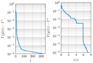
Figure 2: Evolution of the cost error, in logarithmic scale, for the synchronous (left) and node-based asynchronous (right) distributed algorithms.

Then we concentrate on the asynchronous algorithm. In Figure 3 we plot the evolution of the (three) components of the primal variables, $x_{i}^{\star}(t)$, $i\in\{1,\ldots,n\}$. The horizontal dotted lines represent the optimal solution. It is worth noting that the optimal solution has a first component slightly below the constraint boundary, a second component equal to zero, and a third component on the constraint boundary. This optimal solution can be intuitively explained by the “simultaneous influence” of the box constraints (which restrict the set of admissible values) and the regularization term (which enforces sparsity of the vector $x$). In the inset the first iterations for a subset of selected nodes are highlighted, in order to better show the transient, piece-wise constant behavior due to the gossip update and the effect of the box constraint on each component.

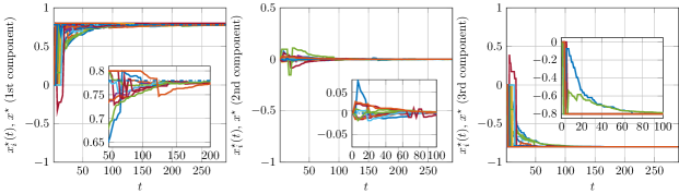
Figure 3: Evolution of the three components of the primal variables $x_{i}^{\star}(t)$, $i\in\{1,\ldots,n\}$, for the node-based Asynchronous Distributed Dual Proximal Gradient.

Specifically, for the first component, it can be seen how the temporary solution of some agents hits the boundary in some iterations (e.g., one of them hits the boundary from iteration $50$ to iteration $100$) and then converges to the (feasible) optimal value. The second components are always inside the box constraint and converge to zero, while the third components start inside the box and then in a finite number of iterations hit the boundary.

VII Conclusions

In this paper we have proposed a class of distributed optimization algorithms, based on dual proximal gradient methods, to solve constrained optimization problems with non-smooth, separable objective functions. The main idea is to construct a suitable, separable dual problem via a proper choice of primal constraints and solve it through proximal gradient algorithms. Thanks to the separable structure of the dual problem in terms of local conjugate functions, a weighted proximal gradient update results into a distributed algorithm, where each node performs a local minimization on its primal variable, and a local proximal gradient update on its dual variables. As main contribution, two asynchronous, event-triggered distributed algorithms are proposed, in which the local updates at each node are triggered by a local timer, without relying on any global iteration counter. The asynchronous algorithms are shown to be special instances of a randomized, block-coordinate proximal gradient method on the dual problem. The convergence analysis is based on a proper combination of duality theory, coordinate-descent methods, and properties of proximal operators.

Giuseppe Notarstefano has been an Assistant Professor (Ricercatore) at the Università del Salento (Lecce, Italy) since February 2007. He received the Laurea degree “summa cum laude” in Electronics Engineering from the Università di Pisa in 2003 and the Ph.D. degree in Automation and Operation Research from the Università di Padova in April 2007. He has been visiting scholar at the University of Stuttgart, University of California Santa Barbara and University of Colorado Boulder. His research interests include distributed optimization, motion coordination in multi-agent networks, applied nonlinear optimal control, and modeling, trajectory optimization and aggressive maneuvering of aerial and car vehicles. He serves as an Associate Editor in the Conference Editorial Board of the IEEE Control Systems Society and for the European Control Conference, IFAC World Congress and IEEE Multi-Conference on Systems and Control. He coordinated the VI-RTUS team winning the International Student Competition Virtual Formula 2012. He is recipient of an ERC Starting Grant 2014.

Ivano Notarnicola has been a Ph.D. student in ”Engineering of Complex Systems” at the Università del Salento (Lecce, Italy) since November 2014. He received the Laurea degree “summa cum laude” in Computer Engineering from the Università del Salento in 2014. He was a visiting student at the Institute of System Theory (Stuttgart, Germany) from March to June 2014. His research interests include distributed optimization and randomized algorithms.

References

- [1] F. Zanella, D. Varagnolo, A. Cenedese, G. Pillonetto, and L. Schenato, “Asynchronous Newton-Raphson consensus for distributed convex optimization,” in 3rd IFAC Workshop on Distributed Estimation and Control in Networked Systems, 2012.
- [2] W. Shi, Q. Ling, G. Wu, and W. Yin, “Extra: An exact first-order algorithm for decentralized consensus optimization,” SIAM Journal on Optimization, vol. 25, no. 2, pp. 944–966, 2015.
- [3] D. Jakovetic, J. M. Freitas Xavier, and J. M. Moura, “Convergence rates of distributed Nesterov-like gradient methods on random networks,” IEEE Transactions on Signal Processing, vol. 62, no. 4, pp. 868–882, 2014.
- [4] A. Nedić and A. Olshevsky, “Distributed optimization over time-varying directed graphs,” vol. 60, no. 3, pp. 601–6015, 2015.
- [5] M. Akbari, B. Gharesifard, and T. Linder, “Distributed subgradient-push online convex optimization on time-varying directed graphs,” in IEEE 52nd Annual Allerton Conference on Communication, Control, and Computing (Allerton), 2014.
- [6] S. S. Kia, J. Cortés, and S. Martínez, “Distributed convex optimization via continuous-time coordination algorithms with discrete-time communication,” Automatica, vol. 55, pp. 254–264, 2015.
- [7] A. I. Chen and A. Ozdaglar, “A fast distributed proximal-gradient method,” in IEEE 50th Annual Allerton Conference on Communication, Control, and Computing (Allerton), 2012, pp. 601–608.
- [8] K. I. Tsianos, S. Lawlor, and M. G. Rabbat, “Consensus-based distributed optimization: Practical issues and applications in large-scale machine learning,” in IEEE 50th Annual Allerton Conference on Communication, Control, and Computing (Allerton), 2012, pp. 1543–1550.
- [9] S. Lee and A. Nedić, “Distributed random projection algorithm for convex optimization,” IEEE Journal of Selected Topics in Signal Processing, vol. 7, no. 2, pp. 221–229, 2013.
- [10] I. Necoara, “Random coordinate descent algorithms for multi-agent convex optimization over networks,” IEEE Transactions on Automatic Control, vol. 58, no. 8, pp. 2001–2012, 2013.
- [11] E. Wei and A. Ozdaglar, “On the convergence of asynchronous distributed alternating direction method of multipliers,” in IEEE Global Conference on Signal and Information Processing (GlobalSIP), 2013, pp. 551–554.
- [12] F. Iutzeler, P. Bianchi, P. Ciblat, and W. Hachem, “Explicit convergence rate of a distributed alternating direction method of multipliers,” arXiv preprint arXiv:1312.1085, 2013.
- [13] P. Bianchi, W. Hachem, and F. Iutzeler, “A stochastic coordinate descent primal-dual algorithm and applications,” in IEEE International Workshop on Machine Learning for Signal Processing (MLSP), 2014, pp. 1–6.
- [14] P. Richtárik and M. Takáč, “Parallel coordinate descent methods for big data optimization,” Mathematical Programming, pp. 1–52, 2015.
- [15] F. Facchinei, G. Scutari, and S. Sagratella, “Parallel selective algorithms for nonconvex big data optimization,” IEEE Transactions on Signal Processing, vol. 63, no. 7, pp. 1874–1889, 2015.
- [16] G. Notarstefano and F. Bullo, “Distributed abstract optimization via constraints consensus: Theory and applications,” vol. 56, no. 10, pp. 2247–2261, 2011.
- [17] M. Bürger, G. Notarstefano, and F. Allgöwer, “A polyhedral approximation framework for convex and robust distributed optimization,” IEEE Transactions on Automatic Control, vol. 59, no. 2, pp. 384–395, 2014.
- [18] A. Beck and M. Teboulle, “A fast iterative shrinkage-thresholding algorithm for linear inverse problems,” SIAM journal on imaging sciences, vol. 2, no. 1, pp. 183–202, 2009.
- [19] Y. Nesterov, “Gradient methods for minimizing composite functions,” Mathematical Programming, vol. 140, no. 1, pp. 125–161, 2013.
- [20] P. Richtárik and M. Takáč, “Iteration complexity of randomized block-coordinate descent methods for minimizing a composite function,” Mathematical Programming, vol. 144, no. 1-2, pp. 1–38, 2014.
- [21] B. O’Donoghue, G. Stathopoulos, and S. Boyd, “A splitting method for optimal control,” IEEE Transactions on Control Systems Technology, vol. 21, no. 6, pp. 2432–2442, 2013.
- [22] Y. Nesterov, “Efficiency of coordinate descent methods on huge-scale optimization problems,” SIAM Journal on Optimization, vol. 22, no. 2, pp. 341–362, 2012.
- [23] I. Necoara and D. Clipici, “Parallel random coordinate descent method for composite minimization: Convergence analysis and error bounds,” SIAM Journal on Optimization, vol. 26, no. 1, pp. 197–226, 2016.
- [24] S. Boyd and L. Vandenberghe, Convex optimization. Cambridge university press, 2004.
- [25] A. Beck and M. Teboulle, “A fast dual proximal gradient algorithm for convex minimization and applications,” Operations Research Letters, vol. 42, no. 1, pp. 1–6, 2014.
- [26] H. H. Bauschke and P. L. Combettes, Convex analysis and monotone operator theory in Hilbert spaces. Springer Science & Business Media, 2011.
- [27] J.-B. Hiriart-Urruty and C. Lemaréchal, “Convex analysis and minimization algorithms ii: Advanced theory and bundle methods,” Grundlehren der mathematischen Wissenschaften, vol. 306, 1993.
- [28] S. Kar and J. M. Moura, “Convergence rate analysis of distributed gossip (linear parameter) estimation: Fundamental limits and tradeoffs,” IEEE Journal of Selected Topics in Signal Processing, vol. 5, no. 4, pp. 674–690, 2011.
- [29] G. M. James, C. Paulson, and P. Rusmevichientong, “The constrained LASSO,” Citeseer, Tech. Rep., 2012.
- [30] H. Xu, D. J. Eis, and P. J. Ramadge, “The generalized lasso is reducible to a subspace constrained lasso,” in IEEE International Conference on Acoustics, Speech and Signal Processing (ICASSP), 2013, pp. 3268–3272.
- [31] N. Parikh and S. Boyd, “Proximal algorithms,” Foundations and Trends in Optimization, vol. 1, no. 3, pp. 123–231, 2013.