March 18, 2024

Lattice Calculation of the Connected Hadronic Light-by-Light Contribution to the Muon Anomalous Magnetic Moment

Luchang Jin,³ Thomas Blum,^1,2 Norman Christ,³ Masashi Hayakawa,³ Taku Izubuchi,³ Christoph Lehner,³

¹ Physics Department, University of Connecticut, Storrs, Connecticut 06269-3046, USA
² RIKEN BNL Research Center, Brookhaven National Laboratory, Upton, New York 11973, USA
³ Physics Department, Columbia University, New York, New York 10027, USA
⁴ Department of Physics, Nagoya University, Nagoya 464-8602, Japan
⁵ Nishina Center, RIKEN, Wako, Saitama 351-0198, Japan
⁶ Physics Department, Brookhaven National Laboratory, Upton, New York 11973, USA

The anomalous magnetic moment of muon, $g-2$, is a very precisely measured quantity. However, the current measurement disagrees with standard model by about 3 standard deviations. Hadronic vacuum polarization and hadronic light by light are the two types of processes that contribute most to the theoretical uncertainty. I will describe how lattice methods are well-suited to provide a first-principle’s result for the hadronic light by light contribution, the various numerical strategies that are presently being used to evaluate it, our current results and the important remaining challenges which must be overcome.

PRESENTED AT

Twelfth Conference on the Intersections of Particle and Nuclear Physics
Vail Colorado at the Vail Marriott from May 19-24, 2015

1 Introduction

The anomalous magnetic moment of muon can be defined in terms of the photon-muon vertex function:

$$\overline{u}(p^{\prime})\Gamma_{\nu}(p^{\prime},p)u(p) = \overline{u}(p^{\prime})\left[F_{1}(q^{2})\gamma_{\nu}+i\frac{F_{2}(q^{2})}{4m_{{\mu}}}[\gamma_{\nu},\gamma_{\rho}]q_{\rho}\right]u(p),$$ (1)

where $F_{2}(0)=(g_{{\mu}}-2)/2\equiv a_{{\mu}}$. The value has been measured very precisely by BNL E821 [3]. It can also be calculated theoretically to great precision as well. [5] Table 1 shows various of theoretical contributions to $a_{{\mu}}$.

Contribution	$\operatorname{Value}\pm\operatorname{Error}$	Ref
QED incl. 5-loops	$116584718.951\pm 0.080$	[1]
HVP LO	$6923\pm 42$	[9]
	$6949\pm 43$	[11]
HVP NLO	$-98.4\pm 0.7$	[11]
Hadronic Light by Light	$105\pm 26$	[15]
Weak incl. 2-loops	$153.6\pm 1.0$	[10]
Standard Model	$116591802\pm 49$	[9]
	$116591828\pm 50$	[11]
Experiment (0.54 ppm)	$116592089\pm 63$	[3]
Difference ($\operatorname{Exp}-\operatorname{SM}$)	$287\pm 80$	[9]
	$261\pm 78$	[11]

Table 1: Comparison between standard model theory and experiment. [in units of $10^{-11}$]

Figure 1: (Left) Hadronic vacuum polarization diagram. (Right) Hadronic light-by-light diagram.

The around three standard deviations between the experiment and theory makes muon $g-2$ a very interesting quantity. A much more accurate experiment by Fermilab E989 is expected in a few years, so a more accurate theoretical determination would be necessary. Figure 1 shows the two diagrams that are the major sources of the theoretical uncertainty.

In this paper, we will only discuss the lattice calculation of connected hadronic light-by-light amplitude. This subject was begun by T. Blum, M. Hayakawa, and T. Izubuchi more than 5 years ago [12, 4]. We have improved the methodology dramatically recently with three major changes. First, we calculate the process at $\mathcal{O}(\alpha^{3})$ with six explicitly internal QED interaction vertices, so no lower order noises or higher order systematic errors will affect our results. Second, we do not generate stochastic QED gauge field configurations, all the photon propagators are calculated exactly based on analytic expressions and Fourier transformations. Third, we compute $F_{2}(q^{2}=0)$ directly in finite volume. A much more accurate result is obtained with the improved method. We then applied this method with simulations parameters closer to physical kinematics.

2 Evaluation Strategy

We start the discussion by spell out the complete expression of the connected light-by-light diagram.

Figure 2: Light-by-Light diagrams. There are 4 other possible permutations.

We denote the momentum carried by the external photon by $\mathbf{q}$. Also, we use Breit-frame, so the initial and final muon states have exactly the same energy,

$$E_{\mathbf{q}/2} = \sqrt{(\mathbf{q}/2)^{2}+m_{{\mu}}^{2}}.$$ (2)

To project each of initial and final states onto a single particle state, we need to take the limits $t_{\text{src}}\rightarrow-\infty$ and $t_{\text{snk}}\rightarrow\infty$. Under these limits, the amplitude in momentum space can be described by the form factors

$$\mathcal{M}^{\text{LbL}}_{\nu}(\mathbf{q}) = e^{i\mathbf{q}\cdot\mathbf{x}_{\text{op}}}\sum_{\mathbf{x}_{\text{snk}},\mathbf{x}_{\text{src}}}e^{-i\mathbf{q}/2\cdot\left(\mathbf{x}_{\text{src}}+\mathbf{x}_{\text{snk}}\right)}e^{E_{\mathbf{q}/2}t_{\text{sep}}}$$ (3)

$$\cdot S_{{\mu}}\left(x_{\text{snk}},x_{\text{op}}\right)\left[F_{1}(q^{2})\gamma_{\nu}+i\frac{F_{2}(q^{2})}{4m}[\gamma_{\nu},\gamma_{\rho}]q_{\rho}\right]S_{{\mu}}\left(x_{\text{op}},x_{\text{src}}\right),$$

where $t_{\text{sep}}=t_{\text{snk}}-t_{\text{src}}$. The above expression is independent of $x_{\operatorname{op}}$, and $\mathcal{M}^{\text{LbL}}$ is only a function of $\mathbf{q}$ as one would expect. In terms of Feynman diagrams, the amplitude is

$$\mathcal{M}^{\text{LbL}}_{\nu}(\mathbf{q}) = e^{i\mathbf{q}\cdot\mathbf{x}_{\text{op}}}\sum_{\mathbf{x}_{\text{snk}},\mathbf{x}_{\text{src}}}e^{-i\mathbf{q}/2\cdot\left(\mathbf{x}_{\text{src}}+\mathbf{x}_{\text{snk}}\right)}e^{E_{\mathbf{q}/2}t_{\text{sep}}}\mathcal{M}^{\text{LbL}}_{\nu}\left(x_{\text{op}},x_{\text{snk}},x_{\text{src}}\right),$$ (4)

$$\mathcal{M}^{\text{LbL}}_{\nu}\left(x_{\text{op}},x_{\text{snk}},x_{\text{src}}\right) = \sum_{x,y,z}\mathcal{F}_{\nu}\left(x,y,z,x_{\text{op}},x_{\text{snk}},x_{\text{src}}\right),$$ (5)

$$\mathcal{F}_{\nu}\left(x,y,z,x_{\text{op}},x_{\text{snk}},x_{\text{src}}\right)$$ (6)

$$= -(-ie)^{6}\sum_{q=u,d,s}(e_{q}/e)^{4}\left\langle\operatorname{tr}\left[\gamma_{\rho}S_{q}(x,z)\gamma_{\kappa}S_{q}(z,y)\gamma_{\sigma}S_{q}\left(y,x_{\text{op}}\right)\gamma_{\nu}S_{q}\left(x_{\text{op}},x\right)\right]\right\rangle_{\text{QCD}}$$

$$\cdot \sum_{x^{\prime},y^{\prime},z^{\prime}}G_{\rho\rho^{\prime}}(x,x^{\prime})G_{\sigma\sigma^{\prime}}(y,y^{\prime})G_{\kappa\kappa^{\prime}}(z,z^{\prime})$$

$$\cdot \left[S_{{\mu}}\left(x_{\text{snk}},x^{\prime}\right)\gamma_{\rho^{\prime}}S_{{\mu}}(x^{\prime},z^{\prime})\gamma_{\kappa^{\prime}}S_{{\mu}}(z^{\prime},y^{\prime})\gamma_{\sigma^{\prime}}S_{{\mu}}\left(y^{\prime},x_{\text{src}}\right)\right.$$

$$+S_{{\mu}}\left(x_{\text{snk}},z^{\prime}\right)\gamma_{\kappa^{\prime}}S_{{\mu}}(z^{\prime},x^{\prime})\gamma_{\rho^{\prime}}S_{{\mu}}(x^{\prime},y^{\prime})\gamma_{\sigma^{\prime}}S_{{\mu}}\left(y^{\prime},x_{\text{src}}\right)$$

$$\left.+\text{other 4 permutations}\right],$$

where $e_{u}/e=2/3$, $e_{d}/e=e_{s}/e=-1/3$.

It is very difficult to evaluate the above complicated three-loop formula directly on the lattice, because we can not afford the $\mathcal{O}\left(\text{Volume}^{2}\right)$ complexity. We need some stochastic method to evaluate the above formula. In Ref [12, 4] we evaluated the quark and muon propagators in the background of quenched QED fields. This will generate all kinds of diagrams, a nice subtraction scheme is then used to subtract all the unwanted pieces, except some higher order terms suppressed by additional powers of $\alpha$.

=

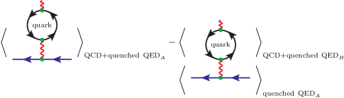
$3\times$

Figure 3: One typical diagram remains after subtraction is shown on the left, 5 others are not shown. See Ref [12, 4] for details.

Although the central value of the lower order terms is subtracted completely, the noise terms is not. After subtraction, the noise is on the order of $\mathcal{O}(e^{4})$ compare with the signal, which is on the order of $\mathcal{O}(e^{6})$. This lower order noise problem can be solved by inserting the stochastic photon explicitly using the sequential source method [13]. Then we would be only evaluating the connected HLbL diagram, without higher order error or lower order noise.

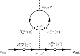
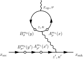
Figure 4: Light-by-Light diagrams calculated with one exact photon and two stochastic photons. There are 4 other possible permutations. See Ref [13] for details.

2.1 Point Source Photon Method

However, there is still a serious problem in the approach above, that is the noise will increase in larger volume. We will call it “disconnected-diagram” problem, because it is similar to the problem one usually encounter when computing diagrams with two or more parts that are not connected by fermion lines on lattice. In our case, the quark loop and the muon line are “disconnected”, so in large volume, lots of noise will be generated from the region where $x^{\prime}$ is far from $x$ or $y^{\prime}$ is far from $y$, since this noise is not suppressed at all.

Use of an analytical photon propagator it contains instead of a stochastic photon field would solve this “disconnected-diagram” problem, but it is not possible to exactly evaluation the full expression because it contains too many loops. As a trade-off, we use two point source photons with sources at $x$ and $y$, which will be chosen randomly. The $8L^{4}$-dimensional stochastic integral over E&M fields will be replaced by a very standard 8-dimensional Monte Carlo integral over two space-time points, and the integrand only depends on the relative position of the two points after QCD ensemble average. To achieve this, we rearrange the expression of the amplitude by defining

$$\mathcal{F}_{\nu}\left(\mathbf{q},x,y,z,x_{\text{op}}\right) = \sum_{\mathbf{x}_{\text{snk}},\mathbf{x}_{\text{src}}}e^{-i\mathbf{q}/2\cdot\left(\mathbf{x}_{\text{src}}+\mathbf{x}_{\text{snk}}\right)}e^{E_{\mathbf{q}/2}t_{\text{sep}}}\mathcal{F}_{\nu}\left(x,y,z,x_{\text{op}},x_{\text{snk}},x_{\text{src}}\right).$$ (7)

Then, we will have

$$\mathcal{M}^{\text{LbL}}_{\nu}(\mathbf{q}) = e^{i\mathbf{q}\cdot\mathbf{x}_{\text{op}}}\sum_{x,y,z}\mathcal{F}_{\nu}\left(\mathbf{q},x,y,z,x_{\text{op}}\right).$$ (8)

Translational invariance of $\mathcal{F}_{\nu}\left(x,y,z,x_{\text{op}},x_{\text{snk}},x_{\text{src}}\right)$ leads to the following equation

$$e^{i\mathbf{q}\cdot\mathbf{x}_{\text{op}}}\mathcal{F}_{\nu}\left(\mathbf{q},x,y,z,x_{\text{op}}\right)$$ (9)

$$= e^{i\mathbf{q}\cdot\left(\mathbf{x}_{\text{op}}-\frac{\mathbf{x}+\mathbf{y}}{2}\right)}\mathcal{F}_{\nu}\left(\mathbf{q},\frac{x-y}{2},-\frac{x-y}{2},z-\frac{x+y}{2},x_{\text{op}}-\frac{x+y}{2}\right).$$

Therefore

$$\mathcal{M}^{\text{LbL}}_{\nu}(\mathbf{q}) = \sum_{x,y,z}e^{i\mathbf{q}\cdot\left(\mathbf{x}_{\text{op}}-\frac{\mathbf{x}+\mathbf{y}}{2}\right)}\mathcal{F}_{\nu}\left(\mathbf{q},\frac{x-y}{2},-\frac{x-y}{2},z-\frac{x+y}{2},x_{\text{op}}-\frac{x+y}{2}\right)$$ (10)

$$= \sum_{r}\left[\sum_{\tilde{z},\tilde{x}_{\text{op}}}e^{i\mathbf{q}\cdot\tilde{\mathbf{x}}_{\text{op}}}\mathcal{F}_{\nu}\left(\mathbf{q},\frac{r}{2},-\frac{r}{2},\tilde{z},\tilde{x}_{\text{op}}\right)\right].$$

where $r=x-y$, $\tilde{z}=z-(x+y)/2$, and $\tilde{x}_{\text{op}}=x_{\text{op}}-(x+y)/2$. This would be the formula suitable for our proposed strategy. The inner sums over $\tilde{z}$ and $\tilde{x}_{\text{op}}$ can be easily summed over the entire lattice as sinks with point source propagators originated at $x$ and $y$. The outer sum will be performed by random sampling the $x$ and $y$ positions. It should be noted that the integrand is sharply peaked in the small $r$ region, so one should sample this region more frequently. In fact, we choose to compute all possible $r$ less than certain limit $r_{\text{max}}$ and simply add them together as the “short distance” contribution. Then, we only randomly sample the region where $r>r_{\text{max}}$, with some probability distribution tailored for the specific pion mass.

There is also a possible $M^{2}$ trick, similar to the one described in Ref [13], which can be applied to this setup in a similar fashion. This trick works as follows. First, one chooses a random point as the reference point $x_{\text{ref}}$. Second, one chooses a set of $M$ points $c_{1}$, $c_{2}$ … $c_{M}$ around $x_{\operatorname{ref}}$ with some pre-specified probability distribution $q(|c_{i}-x_{\operatorname{ref}}|)$. Then, the distance between any two points $x$ and $y$ within this set is given by

$$p(|x-y|) = \sum_{x_{\text{ref}}}q\left(\left|x-x_{\text{ref}}\right|\right)q\left(\left|y-x_{\text{ref}}\right|\right).$$ (11)

With this trick, we obtained $M(M-1)/2$ point pairs by just computing $M$ point source propagators. We have experimented this method on our $32^{3}$ $4.6\mathrm{\operatorname{fm}}$ lattice [2] with a $171\mathrm{\operatorname{MeV}}$ pion and a $134\mathrm{\operatorname{MeV}}$ muon using $M=16$. Under this setting, we found that this $M^{2}$ trick is very effective, all the pairs are almost statistically independent even though they are just different combinations out of the same set of points on the same configuration near the same reference point $x_{\text{ref}}$. This trick can also be applied after including the two following improvements. However, we didn’t use it in our recent numerical studies, because the light quark inversion is made very fast by using Mobius/zMobius fermions [8], the AMA [6] technique, and efficient code [7]. Comparatively, the muon part of the computation, which would need to be performed $M(M-1)/2$ times should we use this $M^{2}$ trick, is quite expensive.

2.2 Conserved External Current Improvement

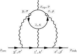
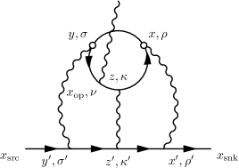
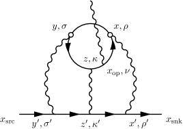
Figure 5: Diagrams showing the three different possible insertions of the external photon when the vertices $x$ and $y$ are fixed. For each of these three diagrams there are five other possible permutations of the connections between the three internal photons and the muon line that are not shown. The contributions of each of these three sets of six contractions will be the same after the stochastic average over the vertices $x$ and $y$. (Left) This is the diagram that we have already calculated. (Middle) We need to compute sequential source propagators at $x_{\text{op}}$ for each polarizations of the external photon. (Right) We also need to compute sequential source propagators at $x_{\text{op}}$, but with the external photon momentum in opposite direction, since we need use $\gamma_{5}$-hermiticity to reverse the direction of the propagators, which reverses the momentum of the external photon as well.

With the point source photon method, the noise for $\mathcal{M}^{\text{LbL}}_{\nu}(\mathbf{q})$ should stay relative constant when we increase the volume of the lattice. However, it should be noticed that the signal of the anomalous magnetic moment is proportion to $q$, so the signal to noise ratio problem in large volume limit remains unless we can control the noise to be proportion to $q$ as well. Recall the reason that the signal proportion to $q$ is the Ward identity, so we should enforce the Ward identity configuration by configuration by including contributions from all the possible external photon insertions, and use the lattice conserved current at $x_{\text{op}}$. After including the three types of diagrams shown in Figure 5, we have

$$\mathcal{F}^{C}_{\nu}\left(x,y,z,x_{\text{op}},x_{\text{snk}},x_{\text{src}}\right)$$

$$\hskip 28.45274pt=\frac{1}{3}\mathcal{F}_{\nu}\left(x,y,z,x_{\text{op}},x_{\text{snk}},x_{\text{src}}\right)+\frac{1}{3}\mathcal{F}_{\nu}\left(y,z,x,x_{\text{op}},x_{\text{snk}},x_{\text{src}}\right)$$

$$\hskip 56.9055pt+\frac{1}{3}\mathcal{F}_{\nu}\left(z,x,y,x_{\text{op}},x_{\text{snk}},x_{\text{src}}\right),$$ (12)

$$\mathcal{F}^{C}_{\nu}\left(\mathbf{q},x,y,z,x_{\text{op}}\right) = \sum_{\mathbf{x}_{\text{snk}},\mathbf{x}_{\text{src}}}e^{-i\mathbf{q}/2\cdot\left(\mathbf{x}_{\text{src}}+\mathbf{x}_{\text{snk}}\right)}e^{E_{\mathbf{q}/2}t_{\text{sep}}}\mathcal{F}^{C}_{\nu}\left(x,y,z,x_{\text{op}},x_{\text{snk}},x_{\text{src}}\right).$$ (13)

We then have a similar formula

$$\mathcal{M}^{\text{LbL}}_{\nu}(\mathbf{q}) = e^{i\mathbf{q}\cdot\mathbf{x}_{\text{op}}}\sum_{x,y,z}\mathcal{F}^{C}_{\nu}\left(\mathbf{q},x,y,z,x_{\text{op}}\right)$$ (14)

$$= \sum_{r}\left[\sum_{\tilde{z},\tilde{x}_{\text{op}}}e^{i\mathbf{q}\cdot\tilde{\mathbf{x}}_{\text{op}}}\mathcal{F}^{C}_{\nu}\left(\mathbf{q},\frac{r}{2},-\frac{r}{2},\tilde{z},\tilde{x}_{\text{op}}\right)\right].$$

There is a side effect of including all three possible external photon insertions. According to the definition Eq. (12), we have $\mathcal{F}^{C}_{\nu}\left(\mathbf{q},x,y,z,x_{\text{op}}\right)=\mathcal{F}^{C}_{\nu}\left(\mathbf{q},y,z,x,x_{\text{op}}\right)=\mathcal{F}^{C}_{\nu}\left(\mathbf{q},z,x,y,x_{\text{op}}\right)$. This allows us to apply another trick,

$$\sum_{x,y,z}\mathcal{F}^{C}_{\nu}\left(\mathbf{q},x,y,z,x_{\text{op}}\right) = \sum_{x,y,z}\mathfrak{Z}\mathcal{F}^{C}_{\nu}\left(\mathbf{q},x,y,z,x_{\text{op}}\right),$$ (15)

where

$$\mathfrak{Z} = \left\{\begin{array}[]{ll}3&\text{if }|x-y|<|x-z|\text{ and }|x-y|<|y-z|\\ 3/2&\text{if }|x-y|=|x-z|<|y-z|\text{ or }|x-y|=|y-z|<|x-z|\\ 1&\text{if }|x-y|=|x-z|=|y-z|\\ 0&\text{otherwise}\end{array}\right..$$ (20)

Following Eq. (14), we obtain

$$\mathcal{M}^{\text{LbL}}_{\nu}(\mathbf{q}) = \sum_{r}\left[\sum_{\tilde{z}}\mathfrak{Z}\sum_{\tilde{x}_{\text{op}}}e^{i\mathbf{q}\cdot\tilde{\mathbf{x}}_{\text{op}}}\mathcal{F}^{C}_{\nu}\left(\mathbf{q},\frac{r}{2},-\frac{r}{2},\tilde{z},\tilde{x}_{\text{op}}\right)\right].$$ (21)

This trick further suppresses contributions from large $|r|$, where most noise would enter, and makes the importance sampling and complete summation of the short distance region more effective.

2.3 Zero External Momentum Transfer Improvement

Recall the basic form of the Ward identity

$$\Delta^{\ast}_{\left(x_{\text{op}}\right)_{\nu}}S_{q}\left(b,x_{\text{op}}\right)\gamma_{\nu}S_{q}\left(x_{\text{op}},a\right) = S_{q}(b,a)\left[\delta\left(x_{\text{op}}-a\right)-\delta\left(x_{\text{op}}-b\right)\right].$$ (22)

Note that the $\gamma_{\nu}$ should be interpreted as a lattice version conserved current at $x_{\text{op}}$. The current conservation formulae

$$\Delta^{\ast}_{\left(x_{\text{op}}\right)_{\nu}}F^{C}_{\nu}\left(x,y,z,x_{\text{op}},x_{\text{snk}},x_{\text{src}}\right) = 0,$$ (23)

$$\Delta^{\ast}_{\left(x_{\text{op}}\right)_{\nu}}\mathcal{F}^{C}_{\nu}\left(\mathbf{q},x,y,z,x_{\text{op}}\right) = 0,$$ (24)

will be true configuration by configuration without discretization error or finite volume error, provided we include all possible external photon insertions and use the lattice version of the conserved current at $x_{\text{op}}$.

With the above formula, we can prove $\sum_{\tilde{x}_{\text{op}}}F_{\nu}^{C}$ vanishes except for terms suppressed exponentially by the lattice size. The reason is that the net total sum of a localized conserved current has to vanish. Mathematically, $F^{C}_{\nu}$ is exponentially suppressed at large $\tilde{x}_{\text{op}}$, therefore we can ignore the surface term in a sufficiently large volume,

$$0 = \sum_{\tilde{x}_{\text{op}}}\Delta^{\ast}_{\left(\tilde{x}_{\text{op}}\right)_{\rho}}\left[\left(\tilde{x}_{\text{op}}\right)_{\nu}\mathcal{F}^{C}_{\rho}\left(\mathbf{q},\frac{r}{2},-\frac{r}{2},\tilde{z},\tilde{x}_{\text{op}}\right)\right]$$ (25)

$$= \sum_{\tilde{x}_{\text{op}}}\left[\mathcal{F}^{C}_{\nu}\left(\mathbf{q},\frac{r}{2},-\frac{r}{2},\tilde{z},\tilde{x}_{\text{op}}\right)+\left(\tilde{x}_{\text{op}}\right)_{\nu}\Delta^{\ast}_{\left(\tilde{x}_{\text{op}}\right)_{\rho}}\mathcal{F}^{C}_{\rho}\left(\mathbf{q},\frac{r}{2},-\frac{r}{2},\tilde{z},\tilde{x}_{\text{op}}\right)\right]$$

$$= \sum_{\tilde{x}_{\text{op}}}\mathcal{F}^{C}_{\nu}\left(\mathbf{q},\frac{r}{2},-\frac{r}{2},\tilde{z},\tilde{x}_{\text{op}}\right),$$

In infinite volume, we can safely subtract above term from our amplitude, we obtain

$$\mathcal{M}^{\text{LbL}}_{\nu}(\mathbf{q}) = \sum_{r}\left[\sum_{\tilde{z},\tilde{x}_{\text{op}}}\left(e^{i\mathbf{q}\cdot\tilde{\mathbf{x}}_{\text{op}}}-1\right)\mathcal{F}^{C}_{\nu}\left(\mathbf{q},\frac{r}{2},-\frac{r}{2},\tilde{z},\tilde{x}_{\text{op}}\right)\right].$$ (26)

Now, the above expression vanishes explicitly when $q\rightarrow 0$. The leading order contribution is

$$\mathcal{M}^{\text{LbL}}_{\nu}(\mathbf{q}) = \sum_{r}\left[\sum_{\tilde{z},\tilde{x}_{\text{op}}}i\mathbf{q}\cdot\tilde{\mathbf{x}}_{\text{op}}\mathcal{F}^{C}_{\nu}\left(\boldsymbol{0},\frac{r}{2},-\frac{r}{2},\tilde{z},\tilde{x}_{\text{op}}\right)\right]+\mathcal{O}(q^{2}).$$ (27)

Matching with Eq. (3), we can see that

$$F_{1}(0) = 0,$$ (28)

$$\sum_{\mathbf{x}_{\text{snk}},\mathbf{x}_{\text{src}}}e^{m_{{\mu}}t_{\text{sep}}}S_{{\mu}}\left(x_{\text{snk}},x_{\text{op}}\right)\left[i\frac{F_{2}(0)}{4m}[\gamma_{\nu},\gamma_{\rho}]q_{\rho}\right]S_{{\mu}}\left(x_{\text{op}},x_{\text{src}}\right)$$ (29)

$$\hskip 142.26378pt=\sum_{r}\left[\sum_{\tilde{z},\tilde{x}_{\text{op}}}i\mathbf{q}\cdot\tilde{\mathbf{x}}_{\text{op}}\mathcal{F}^{C}_{\nu}\left(\boldsymbol{0},\frac{r}{2},-\frac{r}{2},\tilde{z},\tilde{x}_{\text{op}}\right)\right].$$

Now we have an explicit formula about $F_{2}$ at zero momentum transfer. Although the expression is derived in infinite volume, we can still evaluate it in finite volume on the lattice only subject to normal power law finite-volume effects just like other lattice computations include QED. Similarly, although the derivation of Eq. (29) assumes strict current conservation at $x_{\text{op}}$ guaranteed by the lattice version of the conserved current, the final form of the Eq. (29) has no superficial divergence in the ultra-violet region, thus one can also use a local current at $x_{\text{op}}$. Finally, we further simplify the above expression by cancelling $q$ on both sides of the equation,

$$\frac{F_{2}(0)}{m}\sum_{\mathbf{x}_{\text{snk}},\mathbf{x}_{\text{src}}}e^{m_{{\mu}}t_{\text{sep}}}S_{{\mu}}\left(x_{\text{snk}},x_{\text{op}}\right)\frac{\vec{\Sigma}}{2}S_{{\mu}}\left(x_{\text{op}},x_{\text{src}}\right)$$

$$\hskip 56.9055pt=\sum_{r}\left[\sum_{\tilde{z},\tilde{x}_{\text{op}}}\frac{1}{2}\tilde{\mathbf{x}}_{\text{op}}\times i\vec{\mathcal{F}}^{C}\left(\boldsymbol{0},\frac{r}{2},-\frac{r}{2},\tilde{z},\tilde{x}_{\text{op}}\right)\right]$$

$$\hskip 56.9055pt=\sum_{r}\left[\sum_{\tilde{z}}\mathfrak{Z}\sum_{\tilde{x}_{\text{op}}}\frac{1}{2}\tilde{\mathbf{x}}_{\text{op}}\times i\vec{\mathcal{F}}^{C}\left(\boldsymbol{0},\frac{r}{2},-\frac{r}{2},\tilde{z},\tilde{x}_{\text{op}}\right)\right],$$ (30)

where $\Sigma_{i}=\frac{1}{4i}\epsilon_{ijk}[\gamma_{j},\gamma_{k}]$. The evaluation strategy is the same as before. The sum over $\tilde{x}_{\text{op}}$ is performed by the sequential source method. The sum over $\tilde{z}$ is easily evaluated because $\tilde{z}$ is a sink. Again, the final sum over $r$ is performed by random sampling $r$ according to a probability distribution $p(r)$, except for $r\leqslant r_{\text{max}}$ in which case we compute all possible $r$ up to discrete symmetries and sum them with appropriate multiplicity factors.

3 Numerical Studies

In this section we describe three studies. We start by presenting the QED test, computing muon leptonic light-by-light process on lattice and also study the finite volume effects. We then present our $24^{3}$ lattice simulations, which we compare with our previous study in Ref [4]. Finally, we apply our new evaluation strategy to a $32^{3}$ lattice.

3.1 Muon Leptonic Light-by-Light and Finite Volume Effects

We start by using the method described above to compute the muon leptonic light-by-light process. The computation is performed on three different physical volumes and each with three different lattice spacings. The lattice spacing is determined by the physical muon mass, $m_{{\mu}}=106\mathrm{\operatorname{MeV}}$.

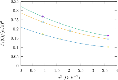
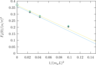
Figure 6: Muon leptonic light by light contribution to muon $g-2$. (Left) Plots of the continuum extrapolation for three different physical lattice sizes $L=11.9\mathrm{\operatorname{fm}}$ (diamonds), $8.9\mathrm{\operatorname{fm}}$ (squares) and $5.9\mathrm{\operatorname{fm}}$ (circles) by assigning $m_{{\mu}}=106\mathrm{\operatorname{MeV}}$. The curves shown are quadratic functions of $a^{2}$ chosen to pass through the three points for each physical volume. (Right) Use the results from the continuum extrapolation to extrapolate to infinite volume. The upper points use the quadratic fit to all three lattice spacing shown in the left plot, while the lower points use a linear fit to the two leftmost points in the left plot. For the upper points, we obtain , we obtain $(0.3679\pm 0.0042)-(1.86\pm 0.11)/(m_{{\mu}}L)^{2}$. For the lower points, we obtain $(0.3608\pm 0.0030)-(1.92\pm 0.08)/(m_{{\mu}}L)^{2}$. The errors are statistical only. For comparison, the analytical formula gives $0.371$. [14]

The finite volume effect implies power-law corrections because of the photon has zero mass and its propagator decreases like $1/r^{2}$. To estimate the finite volume effect in LbL, we study the amplitude as a function of spatial momentum and time, assuming that the effect of excited states has been controlled.

Recall the photon propagator is

$$G(\mathbf{k},t_{2},t_{1}) = \int\frac{\mathrm{d}p_{0}}{2\pi}e^{ip_{0}(t_{2}-t_{1})}\frac{1}{p_{0}^{2}+\mathbf{k}^{2}}$$ (31)

$$= \frac{1}{2|\mathbf{k}|}\exp(-|\mathbf{k}||t_{2}-t_{1}|).$$

For a single internal photon, the behavior of the integrand in small $\mathbf{k}$ region is roughly

$$\int_{-\infty}^{\infty}dt_{\operatorname{line}}\frac{1}{|\mathbf{k}|}\exp(-|\mathbf{k}||t_{\operatorname{loop}}-t_{\operatorname{line}}|)|\mathbf{k}| \sim \mathcal{O}\left(\frac{1}{|\mathbf{k}|}\right),$$ (32)

where $t_{\text{line}}$ represents the time at which the photon couples to the external line and $t_{\text{loop}}$ the location in time of the internal muon loop, fixed by $\left(x_{\text{op}}\right)_{0}$. The last factor of $|\mathbf{k}|$ comes from the fact that the photon has to couple to a neutral loop and the coupling at such a small momentum photon is suppressed by a factor of $|\mathbf{k}|$. Thus, the finite correction should be proportion to

$$\int_{0}^{1/L}\mathcal{O}\left(\frac{1}{|\mathbf{k}|}\right)d^{3}k \sim \mathcal{O}\left(\frac{1}{L^{2}}\right).$$ (33)

This is precisely what we observed in the numerical study. Note that this power-law error is caused by not including the contribution from the region with a large separation between the muon line and the fermion loop correctly. If we simply perform the sum over $x^{\prime}$, $y^{\prime}$, and $z^{\prime}$ in Eq (6)(12) in a larger volume and reuse the point source propagators and contractions for the fermion loop, then we would obtain a smaller finite volume error.

3.2 $333\mathrm{\operatorname{MeV}}$ Pion $24^{3}\times 64$ Lattice

The computation was performed on $18$ configurations each separated by $200$ MD time unit. [2] The muon mass is set to be $175\mathrm{\operatorname{MeV}}$. We compute the short distance part up to $r_{\text{max}}=4$ in lattice unit, and sample the long distance part with the following distribution

$$p_{\text{24IL}}(r) \propto \frac{1}{|r|^{4}}\exp(-0.1|r|).$$ (34)

For each configuration, $118$ pairs are used to compute the short distance part, $128$ pairs are sampled to compute the long distance part.

Our result evaluated with muon source and sink separation $t_{\text{sep}}=32$ is

$$F_{2} = (0.0804\pm 0.0015)\left(\frac{\alpha}{\pi}\right)^{3}.$$ (35)

Because we have precise control of the distance between points $x$ and $y$, we can plot the contribution from each point pair and bin the pairs according to the distance $r$.

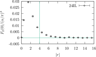
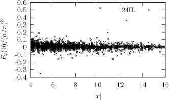
Figure 7: Results from the $24^{3}\times 64$ lattice with $a^{-1}=1.747\mathrm{\operatorname{GeV}}$, $m_{\pi}=333\mathrm{\operatorname{MeV}}$, $m_{{\mu}}=175\mathrm{\operatorname{MeV}}$. $t_{\text{sep}}=32$. (Left) Histogram of the contribution to $F_{2}$ from different separations $r=|x-y|$. The sum of all these points gives the final result for $F_{2}$. (Right) Scatter plot of results for $F_{2}$ for all random point pairs, adjusted by their sampling weight. The average value of $F_{2}$ from all the points gives the $r\geq r_{\max}$ portion of the final result. The vertical line in the left plot and the left-hand boundary of the points shown in the right plot indicate the value of $r_{\max}$.

We compare this value with results obtained in our previous attempt using the subtraction method in Ref [4]. Not only the statistical error becomes much smaller with the new method, the computational cost in terms of the number of quark propagators computed, is also reduced.

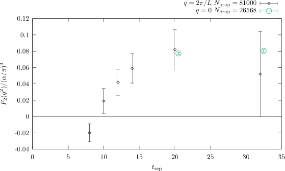
Figure 8: Results from a $24^{3}\times 64$ lattice with $a^{-1}=1.747\mathrm{\operatorname{GeV}}$, $m_{\pi}=333\mathrm{\operatorname{MeV}}$ using $m_{{\mu}}=175\mathrm{\operatorname{MeV}}$. Results from our new methods are shown as red circles. The total cost is $N_{\text{prop}}=26568$ light quark propagators. The small diamonds show the results from our previous calculation in Ref [4] computed with $N_{\text{prop}}=81000$ light quark propagators.

3.3 $171\mathrm{\operatorname{MeV}}$ Pion $32^{3}\times 64$ Lattice

With the more efficient method, we have also attempted a computation on a more physical ensemble, performed on $23$ configurations each separated by $80$ MD time units. [2] The muon mass is set to be $134\mathrm{\operatorname{MeV}}$. We compute the short distance part up to $r_{\text{max}}=5$ in lattice units, and sample the long distance part with the following distribution

$$p_{\text{32ID}}(r) \propto \frac{1}{|r|^{4}}\exp(-0.01|r|).$$ (36)

For each configuration, $217$ pairs are used to compute the short distance part, $512$ pairs are sampled to compute the long distance part.

We use AMA technique to speed up the computations. Figure 9 shows the result from the sloppy solves with $100$ iterations and $550$ low modes. The small correction term $(0.0060\pm 0.0042)(\alpha/\pi)^{3}$, which is computed separately, is then added to obtain our final result for this lattice

$$F_{2} = (0.1054\pm 0.0054)\left(\frac{\alpha}{\pi}\right)^{3}.$$ (37)

This entire computation required $13.2$ BG/Q rack days, where one BG/Q rack is composed of $1024$ nodes each composed of $16$ cores.

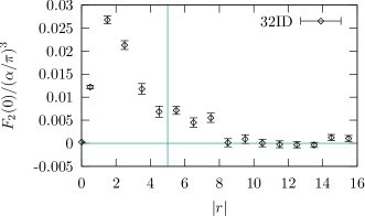
Figure 9: Results from the $32^{3}\times 64$ lattice with $a^{-1}=1.371\operatorname{GeV}$, $m_{\pi}=171\operatorname{MeV}$, $m_{{\mu}}=134\operatorname{MeV}$. $t_{\text{sep}}=32$. (Left) Scatter plot of results for $F_{2}$ for all random point pairs, adjusted by their sampling weight. The average value of $F_{2}$ from all the points gives the $r\geq r_{\max}$ portion of the final result. (Right) Histogram of the contribution to $F_{2}$ from different separations $r=|x-y|$. The sum of all these points gives the final result for $F_{2}$. The vertical line in the right plot and the left-hand boundary of the points shown in the left plot indicate the value of $r_{\max}$.

One may compare this value with the model calculation [15], which gives $(0.08\pm 0.02)(\alpha/\pi)^{3}$, although it should be noted that Eq. (35) and Eq. (37) are computed on lattice with unphysical pion and muon mass, in finite volume, non-zero lattice spacing, and all disconnected diagrams have been omitted.

4 Conclusions

We have made significant improvements to the evaluation strategy of the connected hadronic light-by-light  (cHLbL) diagram. With exact photon propagators and the moment method, one can now compute the connected hadronic light-by-light contribution (cHLbL) to $g-2$ for the muon in the zero momentum transfer limit directly and accurately. The muon leptonic numerical experiments demonstrate the effectiveness of this method, and verify the finite volume error to be  $\mathcal{O}(1/L^{2})$. Using the improved method, we compute the cHLbL on $24^{3}$ $2.71\mathrm{\operatorname{fm}}$ lattice with $333\mathrm{\operatorname{MeV}}$ pion and $175\mathrm{\operatorname{MeV}}$ muon to a greater precision than in our previous result. We also tested this method on a more close-to-physical $32^{3}$ $4.6\mathrm{\operatorname{fm}}$ lattice with a $171\mathrm{\operatorname{MeV}}$ pion and a $134\mathrm{\operatorname{MeV}}$ muon. We are now actively using this method at a physical pion mass and $48^{3}$ $5.5\mathrm{\operatorname{fm}}$ lattice. We also plan to address the finite volume effect and disconnected diagrams within the framework of this newly developed evaluation strategy.

ACKNOWLEDGEMENTS

We would like to thank our RBC and UKQCD collaborators for helpful discussions and support. We would also like to thank RBRC for BG/Q computer. This work was supported in part by US DOE grant DE-SC0011941.

References

- [1] Tatsumi Aoyama, Masashi Hayakawa, Toichiro Kinoshita, and Makiko Nio. Complete Tenth-Order QED Contribution to the Muon g-2. Phys.Rev.Lett., 109:111808, 2012.
- [2] R. Arthur et al. Domain Wall QCD with Near-Physical Pions. Phys. Rev., D87:094514, 2013.
- [3] G.W. Bennett et al. Final Report of the Muon E821 Anomalous Magnetic Moment Measurement at BNL. Phys.Rev., D73:072003, 2006.
- [4] Thomas Blum, Saumitra Chowdhury, Masashi Hayakawa, and Taku Izubuchi. Hadronic light-by-light scattering contribution to the muon anomalous magnetic moment from lattice QCD. Phys.Rev.Lett., 114(1):012001, 2015.
- [5] Thomas Blum, Achim Denig, Ivan Logashenko, Eduardo de Rafael, B. Lee Roberts, et al. The Muon (g-2) Theory Value: Present and Future. 2013.
- [6] Thomas Blum, Taku Izubuchi, and Eigo Shintani. New class of variance-reduction techniques using lattice symmetries. Phys. Rev., D88(9):094503, 2013.
- [7] Peter A. Boyle. The BAGEL assembler generation library. Comput. Phys. Commun., 180:2739–2748, 2009.
- [8] Richard C. Brower, Harmut Neff, and Kostas Orginos. The Móbius Domain Wall Fermion Algorithm. 2012.
- [9] Michel Davier, Andreas Hoecker, Bogdan Malaescu, and Zhiqing Zhang. Reevaluation of the Hadronic Contributions to the Muon g-2 and to alpha(MZ). Eur.Phys.J., C71:1515, 2011.
- [10] C. Gnendiger, D. Stöckinger, and H. Stöckinger-Kim. The electroweak contributions to after the Higgs boson mass measurement. Phys.Rev., D88:053005, 2013.
- [11] Kaoru Hagiwara, Ruofan Liao, Alan D. Martin, Daisuke Nomura, and Thomas Teubner. and alpha() re-evaluated using new precise data. J.Phys., G38:085003, 2011.
- [12] Masashi Hayakawa, Thomas Blum, Taku Izubuchi, and Norikazu Yamada. Hadronic light-by-light scattering contribution to the muon g-2 from lattice QCD: Methodology. PoS, LAT2005:353, 2006.
- [13] Luchang Jin. Lattice Calculation of the Hadronic Light by Light Contributions to the Muon Anomalous Magnetic Moment. PoS, LATTICE2014:130, 2014.
- [14] S. Laporta and E. Remiddi. The Analytic value of the light-light vertex graph contributions to the electron (g-2) in QED. Phys. Lett., B265:182–184, 1991.
- [15] Joaquim Prades, Eduardo de Rafael, and Arkady Vainshtein. Hadronic Light-by-Light Scattering Contribution to the Muon Anomalous Magnetic Moment. 2009.