Unstable manifolds of relative periodic orbits in the symmetry-reduced state space of the Kuramoto-Sivashinsky system

Abstract

Systems such as fluid flows in channels and pipes or the complex Ginzburg-Landau system, defined over periodic domains, exhibit both continuous symmetries, translational and rotational, as well as discrete symmetries under spatial reflections or complex conjugation. The simplest, and very common symmetry of this type is the equivariance of the defining equations under the orthogonal group O(2). We formulate a novel symmetry reduction scheme for such systems by combining the method of slices with invariant polynomial methods, and show how it works by applying it to the Kuramoto-Sivashinsky system in one spatial dimension. As an example, we track a relative periodic orbit through a sequence of bifurcations to the onset of chaos. Within the symmetry-reduced state space we are able to compute and visualize the unstable manifolds of relative periodic orbits, their torus bifurcations, a transition to chaos via torus breakdown, and heteroclinic connections between various relative periodic orbits. It would be very hard to carry through such analysis in the full state space, without a symmetry reduction such as the one we present here.

1 Introduction

“…of course, the motion of the system tends to move away from repellers. Nonetheless a repeller might be important because, for example, it might describe a separatrix that serves to divide two different attractors or two different types of motion.” Kadanoff and Tang KT84 .

The 1984 Kadanoff and Tang investigation of strange repellers was prescient in two ways. First, at the time it was not obvious why anyone would care about “repellers,” as their dynamics would be transient. Today, much of the research in turbulence focuses on repellers. In particular, significant effort is invested in understanding the state space regions of shear-driven fluid flows that separate laminar and turbulent regimes TI03 ; SYE05 ; SchEckYor07 ; duguet07 ; AvMeRoHo13 , and these “separatrices” indeed often appear to be strange repellers. Kadanoff and Tang’s study was quantitative, and modest by today’s standards: they computed escape rates for a family of 3-dimensional mappings in terms of their unstable periodic orbits (‘repulsive cycles’), while today corresponding computations are carried out for very high-dimensional ($\sim$100,000 computational degrees of freedom), numerically accurate discretizetions of Navier-Stokes flows GHCW07 ; channelflow ; openpipeflow . In light of the heuristic nature of their investigation, their second insight was remarkable: they were the first to posit the exact weight for the contribution of an unstable periodic orbit $p$ to an average computed over a strange repeller (or attractor):

$${1}/{\left|\det\left({\bf 1}-J_{p}(x)\right)\right|}$$

(here $J_{p}(x)$ is the Jacobian matrix of linearized flow, computed along the orbit of a periodic point $x$). While, at the time, they were aware only of Bowen’s (1975) work bowen , today this formula is a cornestone of the modern periodic orbit theory of chaos in deterministic flows DasBuch , based on zeta functions of Smale (1967) smale , Gutzwiller (1969) gutzwiller71 , Ruelle (1976) Ruelle76a ; Ruelle76 and their cycle expansions (1987) inv ; AACI ; AACII ; CBook:appendHist . Much has happened since – in particular, the formulas of periodic orbit theory for 3-dimensional dynamics that they had formulated in 1983 are today at the core of the challenge very dear to Kadanoff, a dynamical theory of turbulence Christiansen97 ; GHCW07 . For that to work, many extra moving parts come into play. We have learned that the convergence of cycle expansions relies heavily on the flow topology and the associated symbolic dynamics, and that understanding the geometry of flows in the state space is the first step towards extending periodic orbit theory to systems of high or infinite dimensions, such as fluid flows. It turns out that taking care of the symmetries of a nonlinear fluid flow is also a difficult problem. While one can visualize dynamics in 2 or 3 dimensions, the state space of these flows is high-dimensional, and symmetries -both continuous and discrete- complicate the flow geometry as each solution comes along with all of its symmetry copies. In this contribution to Leo Kadanoff memorial volume, we develop new tools for investigating geometries of flows with symmetries, and illustrate their utility by applying them to a spatiotemporally chaotic Kuramoto-Sivashinsky system.

Originally derived as a simplification of the complex Ginzburg-Landau equation KurTsu76 and in study of flame fronts siv , the Kuramoto-Sivashinsky is perhaps the simplest spatially extended dynamical system that exhibits spatiotemporal chaos. Similar in form to the Navier-Stokes equations, but much easier computationally, the Kuramoto-Sivashinsky partial differential equation (PDE) is a convenient sandbox for developing intuition about turbulence Holmes96 . As for the Navier-Stokes, a state of the Kuramoto-Sivashinsky system is usually visualized by its shape over configuration space (such as states shown in fig. 1). However, the function space of allowable PDE fields is an infinite-dimensional state space, with the instantaneous state of the field a point in this space. In spite of the state space being of high (and even infinite) dimension, evolution of the flow can be visualized, as generic trajectories are 1-dimensional curves, and numerically exact solutions such as equilibria and periodic orbits are points or closed loops, in any state space projection. There are many choices of a “state space.” Usually one starts out with the most immediate one: computational elements used in a finite-dimensional discretization of the PDE studied. As the Kuramoto-Sivashinsky system in one space dimension, with periodic boundary condition, is equivariant under continuous translations and a reflection, for the case at hand the natural choice is a Fourier basis, truncated to a desired numerical accuracy. This is still a high-dimensional space: in numerical work performed here, $30$-dimensional. For effective visualizations, one thus needs to carefully pick dynamically intrinsic coordinate frames, and projections on them SCD07 ; GHCW07 .

Such dynamical systems visualisations of turbulent flows, complementary to the traditional spatio-temporal visualizations, offer invaluable insights into the totality of possible motions of a turbulent fluid. However, symmetries, and especially continuous symmetries, such as equvariance of the defining equations under spatial translations, tend to obscure the state space geometry of the system by their preference for higher-dimensional invariant $N$-tori solutions, such as relative equilibria and relative periodic orbits.

In order to avoid dealing with such effects of continuous symmetry, a number of papers Christiansen97 ; RCMR04 ; ReCi05 ; lanCvit07 ; ReChMi07 study the Kuramoto-Sivashinsky equation within the flow-invariant subspace of solutions symmetric under reflection. However, such restrictions to flow-invariant subspaces miss the physics of the problem: any symmetry invariant subspace is of zero measure in the full state space, so a generic turbulent trajectory explores the state space outside of it. Lacking continuous-symmetry reduction schemes, earlier papers on the geometry of the Kuramoto-Sivashinsky flow in the full state space ksgreene88 ; AGHks89 ; KNSks90 ; SCD07 were restricted to the study of the smallest invariant structures: equilibria, their stable/unstable manifolds, their heteroclinic connections, and their bifurcations under variations of the domain size.

Stationary solutions are important for understanding the state space geometry of a chaotic attractor, as their stable manifolds typically set the boundaries of the strange set. The Lorenz attractor is the best known example Williams79 and Gibson et al. GHCW07 visualizations for the plane Couette flow are so far the highest-dimensional setting, where this claim appears to hold. In this paper we turn our attention to (relative) periodic orbits, which –unlike unstable equilibria– are embedded within the strange set, and are expected to capture physical properties of an ergodic flow. Refs. Christiansen97 ; lanCvit07 , restricted to the reflection-invariant subspace of the Kuramoto-Sivashinsky flow, have succeeded in constructing symbolic dynamics for several system sizes. In these examples, short periodic orbits have real Floquet multipliers, with very thin unstable manifolds, around which the longer periodic orbits are organized by means of nearly 1-dimensional Poincaré  return maps.

In this paper we study the unstable manifolds of relative periodic orbits of Kuramoto-Sivashinsky system in full state space, with no symmetry restrictions. In contrast to the flow-invariant subspace considered in refs. Christiansen97 ; lanCvit07 , the shortest relative periodic orbit of the full system that is stable for small system sizes ($L<21.22$) has a complex leading Floquet multiplier. This renders the associated unstable manifold 2-dimensional. Elimination of the marginal directions, the space and time translation symmetries, by a ‘slice’ and a Poincaré section conditions, together with a novel reduction of the spatial reflection symmetry, enables us to study here this 2-dimensional unstable manifold. We compute and visualize the unstable manifold of the shortest periodic orbit as we increase the system size towards the system’s transition to chaos.

Summary of our findings is as follows: At the system size $L\approx 21.22$, the shortest periodic orbit undergoes a torus bifurcation hopf42 (also sometimes referred to as the Neimark-Sacker bifurcation Neimark59 ; Sacker65 , if the flow is studied in a Poincaré section), which gives birth to a stable 2-torus. As the system size is increased, this torus first goes unstable, and is eventually destroyed by the bifurcation into stable and unstable pair of period-$3$ orbits, to which the unstable manifold of the parent orbit is heteroclinically connected. As the system size is increased further, the stable period-$3$ orbit goes unstable, then disappears, and the dynamics becomes chaotic. Upon a further increase of the system size, the unstable period $3$ orbit undergoes a symmetry-breaking bifurcation, which introduces richer dynamics as the associated unstable manifold has connections to both drifting (relative) and non-drifting periodic orbits.

We begin by a short review of the Kuramoto-Sivashinsky system in the next section, and review continuous symmetry reduction by first Fourier mode slice method in section 3.1. The main innovation introduced in this paper is the invariant polynomial discrete symmetry reduction method described in section 3.2. The new symmetry reduction method is applied to and tested on the Kuramoto-Sivashinsky system in section 4, where the method makes it possible to track the evolution of the periodic orbits unstable manifolds through the system’s transition to chaos. We discuss the implications of our results and possible future directions in section 5.

2 Kuramoto-Sivashinsky system and its symmetries

We study the Kuramoto-Sivashinsky equation in one space dimension

$$u_{\tau}=-u\,u_{x}-u_{xx}-u_{xxxx}\,,$$ (1)

with periodic boundary condition $u(x,\tau)=u(x+L,\tau)$. The real field $u(x,\tau)$ is the “flame front” velocity siv . The domain size $L$ is the bifurcation parameter for the system, which exhibits spatiotemporal chaos for sufficiently large $L$: see fig. 1 (e) for a typical spatiotemporally chaotic trajectory of the system at $L=22$.

\begin{overpic}[height=130.08731pt]{ksRecycled-ConfEq2} \put(-0.75,-1.0){(a)} \end{overpic}

\begin{overpic}[height=130.08731pt]{ksRecycled-ConfTW1} \put(-0.75,-1.0){(b)} \end{overpic}

\begin{overpic}[height=130.08731pt]{ksRecycled-ConfPpo} \put(-0.75,-1.0){(c)} \end{overpic}

\begin{overpic}[height=130.08731pt]{ksRecycled-ConfRpo} \put(-0.75,-1.0){(d)} \end{overpic}

\begin{overpic}[height=130.08731pt]{ksRecycled-ConfErgodic} \put(-0.75,-1.0){(e)} \end{overpic}

Figure 1: Examples of invariant solutions of the Kuramoto-Sivashinsky system and the chaotic flow visualized as the color coded amplitude of the scalar field $u(x,\tau)$: (a) Equilibrium $E_{1}$, (b) Relative equilibrium $TW_{1}$, (c) Pre-periodic orbit with period $T=32.4$, (d) Relative periodic orbit with period $T=33.5$ . (e) Chaotic flow. Horizontal and vertical axes correspond to space and time respectively. System size $L=22$. The invariant solutions and their labels are taken from ref. SCD07 .

We discretize the Kuramoto-Sivashinsky system by Fourier expanding the field $u(x,\tau)=\sum_{k}\tilde{u}_{k}(\tau)e^{iq_{k}x}\,,$ and expressing (1) in terms of Fourier modes as an infinite set of ordinary differential equations (ODEs)

$$\dot{\tilde{u}}_{k}=(q_{k}^{2}-q_{k}^{4})\,\tilde{u}_{k}-i\frac{q_{k}}{2}\!\sum_{m=-\infty}^{+\infty}\!\!\tilde{u}_{m}\tilde{u}_{k-m}\,,\quad q_{k}=\frac{2\pi k}{L}\,.$$ (2)

Kuramoto-Sivashinsky equation is Galilean invariant: if $u(x,\tau)$ is a solution, then $v+u(x-v\tau,\tau)$, with $v$ an arbitrary constant velocity, is also a solution. In the Fourier representation (2), the Galilean invariance implies that the zeroth Fourier mode $\tilde{u}_{0}$ is decoupled from the rest and time-invariant. Hence, we exclude $\tilde{u}_{0}$ from the state space and represent a Kuramoto-Sivashinsky state $u=u(x,\tau)$ by the Fourier series truncated at $k\!=\!N$, i.e., a $2N$-dimensional real valued state space vector

$$a=(b_{1},c_{1},b_{2},c_{2},\dots,b_{N},c_{N})\,,$$ (3)

where $b_{k}={\rm Re}\,[\tilde{u}_{k}]$, $c_{k}={\rm Im}\,[\tilde{u}_{k}]$. One can rewrite (2) in terms of this real valued state space vector, and express the truncated set of equations compactly as

$$\dot{a}=v(a)\,.$$ (4)

In our numerical work we use a pseudo-spectral formulation of (4), described here in appendix A, and in detail in the appendix of ref. SCD07 .

Spatial translations $u(x,\tau)\rightarrow u(x+\delta x,\tau)$ on a periodic domain correspond to $\textrm{SO}(2)$ rotations $a\to{D}(g(\theta))\,a$ in the Kuramoto-Sivashinsky state space, with the matrix representation

$${D}(g(\theta))=\mathrm{diag}\left[\,{}R(\theta),\,R(2\theta),\,\ldots,\,R(N\theta)\,\right]\,,$$ (5)

where $\theta=2\pi\delta x/L$ and

$$R(k\theta)=\begin{pmatrix}\cos k\theta&-\sin k\theta\\ \sin k\theta&~{}\cos k\theta\end{pmatrix}$$

are $[2\!\times\!2]$ rotation matrices. Kuramoto-Sivashinsky dynamics commutes with the action of (5), as can be verified by checking that (4) satisfies the equivariance relation

$$v(a)={D}^{-1}(g(\theta))v({D}(g(\theta))a)\,.$$ (6)

By the translation symmetry of the Kuramoto-Sivashinsky system, each solution of PDE (1) has infinitely many dynamically equivalent copies that can be obtained by translations (5). Systems with continuous symmetries thus tend to have higher-dimensional invariant solutions: relative equilibria (traveling waves) and relative periodic orbits. A relative equilibrium evolves only along the continuous symmetry direction

$$a_{tw}(\tau)={D}(g(\tau\,\dot{\theta}_{tw}))\,a_{tw}(0)\,,$$

where $\dot{\theta}_{tw}$ is a constant phase velocity, and the suffix $\scriptsize{tw}$ indicates that the solution is a “traveling wave.” A relative periodic orbit recurs exactly at a symmetry-shifted location after one period

$$a_{rp}(0)={D}(g(-\theta_{rp}))\,a_{rp}({T_{rp}})\,.$$ (7)

Fig. 1 (b) and (d) show space-time visualizations of a Kuramoto-Sivashinsky relative equilibrium and a relative periodic orbit. The sole dynamics of a relative equilibrium is a constant drift along the continuous symmetry direction, while a relative periodic orbit shifts by amount $\theta_{rp}$ for each repeat of its period, and traces out a torus in the full state space.

The Kuramoto-Sivashinsky equation (1) has no preferred direction, and is thus also equivariant under the reflection symmetry $u(x,\tau)\rightarrow-u(-x,\tau)$: for each solution drifting left, there is a reflection-equivalent solution which drifts right. In terms of Fourier components, the reflection $\sigma$ acts as complex conjugation followed by a negation, whose action on vectors in state space (3) is represented by the diagonal matrix

$${D}(\sigma)=\mathrm{diag}\left[\,-1,\,1,\,-1,\,1,\,\ldots,\,-1,\,1\right]\,,$$ (8)

which flips signs of the real components $b_{i}$. Due to this reflection symmetry, the Kuramoto-Sivashinsky system can also have strictly non-drifting equilibria and (pre-)periodic orbits. An equilibrium is a stationary solution $a_{eq}(\tau)=a_{eq}(0)\,.$ A periodic orbit $p$ is periodic with period $T_{p}$, $a_{p}(0)=a({T_{p}})\,,$ and a pre-periodic orbit is a relative periodic orbit

$$a_{pp}(0)={D}(\sigma)\,a_{pp}({T_{pp}})$$ (9)

which closes in the full state space after the second repeat, hence we refer to it here as ‘pre-periodic’.

In fig. 1 (a) we show equilibrium $E_{1}$ of Kuramoto-Sivashinsky equation (so labelled in ref. SCD07 ). If we were to take the mirror image of fig. 1 (a) with respect to $x=0$ line, and then interchange red and blue colors, we would obtain the same solution; all equilibria belong to the flow-invariant subspace of solutions invariant under the reflection symmetry of the Kuramoto-Sivashinsky equation. Similar to equilibria, time-periodic solutions of the Kuramoto-Sivashinsky equation that are not repeats of pre-periodic ones (9) also belong to the reflection-invariant subspace. See  Christiansen97 ; RCMR04 ; ReCi05 ; lanCvit07 ; ReChMi07 for examples of such solutions. Fig. 1 (b) shows a pre-periodic solution of the Kuramoto-Sivashinsky system: dynamics of the second period can be obtained from the first one by reflecting it. Both equilibria and pre-periodic orbits have infinitely many copies that can be obtained by continuous translations, symmetric across the shifted symmetry line, $g(\theta)\sigma g(-\theta)$. Note that reflection $\sigma$ and translations $g(\theta)$ do not commute: $\sigma\,g(\theta)=-g(\theta)\,\sigma\,,$ or, in terms of the generator of translations, the reflection reverses the direction of the translation, $\sigma\,T=-T\,\sigma$. Let ${f^{\tau}(a)}$ denote the finite-time flow induced by (4), and let $a_{pp}$ belong to a pre-periodic orbit  defined by (9). Then the shifted point $a_{pp}^{\prime}={D}(g(\theta))\,a_{pp}$ satisfies

$${f^{{T_{p}}}(a_{pp}^{\prime})}={D}(g(\theta)){D}(\sigma){D}(g(-\theta))\,a_{pp}^{\prime}\,.$$

In contrast, a relative periodic orbit (7) has a distinct reflected copy $a_{rp}^{\prime}={D}(\sigma)a_{rp}$ with the reverse phase shift:

$$a_{rp}^{\prime}(0)={D}(g(\theta_{p}))\,a_{rp}^{\prime}({T_{p}})\,.$$

In order to carry out our analysis, we must first eliminate all these degeneracies. This we do by symmetry reduction, which we describe next.

3 Symmetry reduction

A group orbit of state $a$ is the set of all state space points reached by applying all symmetry actions to $a$. Symmetry reduction is any coordinate transformation that maps each group orbit to a unique state space point $\tilde{a}$ in the symmetry-reduced state space. For the $\textrm{O}(2)$ symmetry considered here, we achieve this in two steps: We first reduce continuous translation symmetry of the system by method of slices, and then reduce the remaining reflection symmetry by constructing an invariant polynomial basis.

To the best of our knowledge, Cartan CartanMF was first to use method of slices in purely differential geometry context and early appearances of slicing methods in dynamical systems literature are works of Field Field80 and Krupa Krupa90 . Our implementation of the method of slices for $\textrm{SO}(2)$ symmetry reduction follows ref. BudCvi14 . For a more exhaustive review of the literature we refer the reader to ref. DasBuch .

Invariant polynomial or ‘integrity’ bases gatermannHab ; ChossLaut00 are a standard tool Hilbert93 ; Noether15 for orbit space reduction. They work very well in low dimensions ChossLaut00 ; GL-Gil07b ; SiCvi10 ; BuBoCvSi14 , but in high dimensions integrity bases are high-order polynomials of the original state space coordinates, accompanied by large numbers of nonlinear syzygies that confine the symmetry-reduced dynamics to lower-dimensional manifolds. These make the geometry of the reduced state space complicated and hard to work with for applications we have in mind here, such as visualizations of unstable manifolds of invariant solutions. Even with the use of computer algebra gatermannHab , constructing an $\textrm{O}(2)$-invariant integrity basis becomes impractical for systems of dimension higher than $\sim 12$. In spatio-temporal and fluid dynamics applications the corresponding $n$ (Fourier series truncation) is easily of order 10-100. The existing methods for construction of such integrity bases are neither feasible for higher-dimensional state spaces SiminosThesis (we need to reduce symmetry for $10^{5}$-$10^{6}$-dimensional systems GHCW07 ; ACHKW11 ), nor helpful for reduced state space visualizations ($m$-th Fourier coefficient is usually replaced by a polynomial of order $m$).

Here we avoid constructing such high-order $\textrm{O}(2)$ polynomial integrity bases by a hybrid approach. We reduce the continuous symmetry by the first Fourier mode slice in section 3.1, and then reduce the remaining reflection symmetry by a transformation to invariant polynomials in section 3.2. The resulting polynomials are only second order in the original state space coordinates, with no syzygies.

3.1 $\textrm{SO}(2)$ symmetry reduction

Following ref. BudCvi14 , we reduce the $\textrm{SO}(2)$ symmetry of the Kuramoto-Sivashinsky equation by implementing the first Fourier mode slice method, i.e., by rotating the Fourier modes as

$$\hat{a}(\tau)={D}(g(\phi(\tau))^{-1})\,a(\tau)\,,$$ (10)

where $\phi(\tau)=\arg(\tilde{u}_{1}(\tau))$ is the phase of the first Fourier mode. This transformation exists as long as the first mode in the Fourier expansion (10) does not vanish, $b_{1}^{2}+c_{1}^{2}>0$, and its effect is to fix the phase of the first Fourier mode to zero for all times, as illustrated in fig. 2. The $\textrm{SO}(2)$-reduced state space is one dimension lower than the full state space, with coordinates

$$\hat{a}=(\hat{b}_{1},0,\hat{b}_{2},\hat{c}_{2},\ldots\hat{b}_{N},\hat{c}_{N})\,.$$ (11)

The dynamics within the first Fourier mode slice is given by

$$\dot{\hat{a}}=\hat{v}(\hat{a})=v(\hat{a})-\frac{\dot{c}_{1}}{\hat{b}_{1}}\,T\hat{a}\,,$$ (12)

where $T$ is the generator of infinitesimal $\textrm{SO}(2)$ transformations, ${D}(g(\theta))=\exp T\theta$, and $\dot{c}_{1}$ is full state space orbit’s out-of-slice velocity, the second element of the velocity field (4). Symmetry-reduced state space velocity (12) diverges when the amplitude $\hat{b}_{1}$ of the first Fourier mode tends to $0$. If $\hat{b}_{1}$ were $0$, then the transformation (10) would no longer be uniquely defined. However, our experience had been such that this does not happen for generic trajectories of a chaotic system; and the singularity in the vicinity of $\hat{b}_{1}=0$ can be regularized by a time-rescaling transformation BudCvi14 . For further details we refer the reader to refs. DasBuch ; BudCvi14 ; BuBoCvSi14 .

[capbesideposition=left,center,capbesidewidth=0.4]figure[]

Figure 2: A sketch of the full state space trajectory $a(\tau)$ (blue and red) projected onto the first Fourier mode subspace $(b_{1},c_{1})$, with rotation phases $\phi(\tau_{1})$, $\phi(\tau_{2})$ at times $\tau_{1}$ and $\tau_{2}$, see (10). In this 2-dimensional projection we are looking at the symmetry-reduced state space “from the top”; the symmetry-reduced orbit is confined to the horizontal half-axis $(\hat{b}_{1}>0,\,\hat{c}_{1}=0)$ , and the remaining $2N\!-\!2$ coordinates are all projected onto the origin.

3.2 $\textrm{O}(2)$ symmetry reduction

Our next challenge is to devise a transformation from (11) to discrete-symmetry-reduced coordinates, where the equivariance under reflection is also reduced. Consider the action of reflection on the $\textrm{SO}(2)$-reduced state space. In general, a slice is an arbitrarily oriented hyperplane, and action of the reflection $\sigma$ can be rather complicated: it maps points within the slice hyperplane into points outside of it, which then have to be rotated into the slice. However, the action of $\sigma$ on the first Fourier mode slice is particularly simple. Reflection operation ${D}(\sigma)$ of (8) flips the sign of the first $\textrm{SO}(2)$-reduced state space coordinate in (11), i.e., makes the phase of the first Fourier mode $\pi$. Rotating back into the slice by (10), we find that within the first Fourier mode slice, the reflection acts by alternating the signs of even (real part) and odd (imaginary part) Fourier modes:

$$\hat{{D}}(\sigma) = {D}(g(-\pi)){D}(\sigma)$$ (13)

$$= \mathrm{diag}\left[\,1,\,-1,\,-1,\,1,\,1,\,-1,\,-1,\,1,\,1,\,\ldots\right]\,.$$

The action on the slice coordinates (where we for brevity omit all terms whose signs do not change under reflection) is thus

$$\hat{{D}}(\sigma) (\hat{b}_{2},\hat{c}_{3},\hat{b}_{4},\hat{c}_{5},\hat{b}_{6},\hat{c}_{7},\ldots)$$ (14)

$$=(-\hat{b}_{2},-\hat{c}_{3},-\hat{b}_{4},-\hat{c}_{5},-\hat{b}_{6},-\hat{c}_{7},\ldots)\,.$$

Our task is now to construct a transformation to a set of coordinates invariant under (14). One could declare a half of the symmetry-reduced state space to be a ‘fundamental domain’ DasBuch , with segments of orbits that exit it brought back by reflection, but this makes orbits appear discontinuous and the dynamics hard to visualize. Instead, here we shall reduce the reflection symmetry by constructing polynomial invariants of coordinates (14). Squaring (or taking absolute value of) each sign-flipping coordinate in (14) is not an option, since such coordinates would be invariant under every individual sign change of these coordinates, and that is not a symmetry of the system. We are allowed to impose only one condition to reduce the 2-element group orbit of the discrete reflection subgroup of $\textrm{O}(2)$. How that can be achieved is suggested by Miranda and Stone GL-Mir93 ; GL-Gil07b reduction of $\textrm{C}_{2}$ symmetry $(x,y,z)\rightarrow(-x,-y,z)$ of the Lorenz flow. They construct the symmetry-reduced “proto-Lorenz system” by transforming coordinates to the polynomial basis

$$u=x^{2}-y^{2}\,,\quad v=2xy\,,\quad z=z\,.$$ (15)

The $x$ coordinate can be recovered from $u$ and $v$ of (15) up to a choice of sign, i.e., up to the original reflection symmetry. We extend this approach in order to achieve a $2\!-\!\mbox{to}\!-\!1$ symmetry reduction for Kuramoto-Sivashinsky system: we construct the first coordinate from squares, but then ‘twine’ the successive sign-flipping terms $(\hat{b}_{2},\hat{c}_{3},\hat{b}_{4},\hat{c}_{5},\hat{b}_{6},\hat{c}_{7},\ldots)$ into second-order invariant polynomials basis set

$$(p_{2},p_{3},p_{4},p_{5},p_{6},\ldots)$$

$$=(\hat{b}_{2}^{2}-\hat{c}_{3}^{2},\,\hat{b}_{2}\hat{c}_{3},\,\hat{b}_{4}\hat{c}_{3},\,\hat{b}_{4}\hat{c}_{5},\,\hat{b}_{5}\hat{c}_{6},\,\ldots)\,.$$ (16)

The original coordinates can be recovered recursively by the $1\!-\!\mbox{to}\!-\!2$ inverse transformation

$$b_{2} = \pm\sqrt{\frac{p_{2}+\sqrt{p_{2}^{2}+4p_{3}^{2}}}{2}}$$

$$c_{3} = p_{3}/b_{2}\,,\quad b_{4}\,=\,p_{4}/c_{3}\,,\quad c_{5}\,=\,p_{5}/b_{4}\,,\quad\cdots\,.$$

To summarize: we first reduce the group orbits generated by the continuous $\textrm{SO}(2)$ symmetry subgroup by implementing the first Fourier mode slice (10), and then reduce the group orbits of the discrete 2-element reflection subgroup by replacing the sign-changing coordinates (14) with the invariant polynomials (16). The final $\textrm{O}(2)$ symmetry-reduced coordinates are

$$\tilde{a}=(\hat{b}_{1},0,\hat{b}_{2}^{2}-\hat{c}_{3}^{2},\hat{c}_{2},\hat{b}_{3},\hat{b}_{2}\hat{c}_{3},\hat{b}_{4}\hat{c}_{3},\hat{c}_{4},\hat{b}_{5},\ldots)\,.$$ (17)

Here pairs of orbits related by reflection $\sigma$ are mapped into a single orbit, and $\hat{c}_{1}$ is identically set to $0$ by continuous symmetry reduction, thus the symmetry-reduced state space has one dimension less than the full state space.

The symmetry-reduced state space (17) retains all physical information of the Kuramoto-Sivashinsky system: relative equilibria and relative periodic orbits of the original system become equilibria and periodic orbits in the symmetry-reduced state space (17), and pre-periodic orbits close after one period. For this reason, in what follows we shall refer to both relative periodic orbits and pre-periodic orbits as ‘periodic orbits’, unless we comment on their specific symmetry properties.

4 Unstable manifolds of periodic orbits

In order to demonstrate the utility, and indeed, the necessity of the $\textrm{O}(2)$ symmetry reduction, we now investigate the transition to chaos in the neighborhood of a short Kuramoto-Sivashinsky pre-periodic orbit, focusing on the parameter range $L\in[21.0,21.7]$. Our method yields a symmetry-reduced velocity field $\tilde{v}(\tilde{a})=\dot{\tilde{a}}$ and a finite-time flow ${\tilde{f}^{\tau}(\tilde{a}(0))}=\tilde{a}(\tau)$ in the symmetry-reduced state space (17). Although we can obtain $\tilde{v}(\tilde{a})$ by chain rule, we find its numerical integration unstable, hence in practice we obtain $\tilde{v}(\tilde{a})$ and ${\tilde{f}^{\tau}(\tilde{a})}$ from the first Fourier mode slice by applying the appropriate Jacobian matrices, as described in appendix A.

Table 1: The two leading non-marginal Floquet multipliers $\Lambda=\exp({T}\mu+i\theta)$ of periodic orbits $p_{0}$, $p_{1}$, $p_{2}$ for system sizes $L$ studied here. Dash – indicates that the orbit is not found for the corresponding system size.

	$p_{0}$		$p_{1}$		$p_{2}$
L	$\mu$	$\theta$	$\mu$	$\theta$	$\mu$	$\theta$
21.25	$6.443\times 10^{-4}$	$\pm 2.177$	–		–
21.30	$1.839\times 10^{-3}$	$\pm 2.158$	–		–
21.36	$1.839\times 10^{-3}$	$\pm 2.158$	$5.854\times 10^{-3}$	$0$	$-1.623\times 10^{-3}$	$\pm 0.3098$
			$-8.357\times 10^{-3}$	$0$
21.48	$7.638\times 10^{-3}$	$\pm 2.097$	$1.307\times 10^{-2}$	$0$	–
			$-1.234\times 10^{-2}$	$0$
21.70	$1.739\times 10^{-2}$	$\pm 2.044$	$2.521\times 10^{-2}$	$0$	–
			$4.157\times 10^{-3}$	$\pi$

At $L=21.0$, the Kuramoto-Sivashinsky system has a stable periodic orbit $p_{0}$, which satisfies $\tilde{a}_{p_{0}}={\tilde{f}^{{T_{p_{0}}}}(\tilde{a}_{p_{0}})}$ for any point $\tilde{a}_{p_{0}}$ on the periodic orbit $p_{0}$. Linear stability of a periodic orbit  is described by the Floquet multipliers $\Lambda_{i}$ and Floquet vectors $\tilde{V}_{i}$,1 which are the eigenvalues and eigenvectors of the Jacobian matrix $\tilde{J}_{p}$ of the finite-time flow ${\tilde{f}^{{T_{p}}}(\tilde{a}_{p})}$

$$\tilde{J}_{p}\tilde{V}_{i}=\Lambda_{i}\tilde{V}_{i}\,.$$

Each periodic orbit has at least one marginal Floquet multiplier $\Lambda_{v}=1$, corresponding to the velocity field direction. When $L<21.22$, all other Floquet multipliers of $p_{0}$ have absolute values less than $1$. At $L\approx 21.22$, leading complex pair of Floquet multipliers $\Lambda_{1,2}$ crosses the unit circle, and the corresponding eigenplane spanned by the real and imaginary parts of $\tilde{V}_{1}$ develops ‘spiral out’ dynamics that connects to a $2$-torus.

\begin{overpic}[height=195.12767pt]{PPO1Poincare} \put(-0.75,-1.0){(a)} \end{overpic}

\begin{overpic}[height=195.12767pt]{PsectL21p25} \put(-0.75,-1.0){(b)} \end{overpic}

Figure 3: (a) Pre-periodic orbit $p_{0}$ (red), its velocity field $\tilde{v}(\tilde{a}_{p_{0}})$ at the starting point (green), orthogonal vectors that span the eigenplane corresponding to the leading Floquet vectors (blue) and the Poincaré section hyperplane (gray, transparent). (b) Spiral-out dynamics of a single trajectory in the Poincaré section projected onto $(e_{1},e_{2})$ plane, system size $L=21.25$.

In order to study dynamics within the neighborhood of $p_{0}$, we define a Poincaré section as the hyperplane of points $\tilde{a}_{{\cal P}}$ in an open neighborhood of $\tilde{a}_{p_{0}}$, orthogonal to the tangent $\tilde{v}(\tilde{a}_{p_{0}})$ of the orbit at the Poincaré section point,

$$(\tilde{a}_{{\cal P}}-\tilde{a}_{p_{0}})\cdot\tilde{v}(\tilde{a}_{p_{0}})=0\quad\mbox{and}\quad||\tilde{a}_{{\cal P}}-\tilde{a}_{p_{0}}||<\alpha\,,$$ (18)

where $||.||$ denotes the Euclidean (or $L2$) norm, and the threshold $\alpha$ is empirically set to $\alpha=0.9$ throughout. The locality condition in (18) is a computationally convenient way to avoid Poincaré section border atlas12 ; DasBuch , defined as the set of points $\tilde{a}_{{\cal P}}^{*}$ that satisfy the hyperplane condition $(\tilde{a}_{{\cal P}}^{*}-\tilde{a}_{p_{0}})\cdot\tilde{v}(\tilde{a}_{p_{0}})=0$ , but their orbits do not intersect this hyperplane transversally, i.e. $\tilde{v}(\tilde{a}_{{\cal P}}^{*})\cdot\tilde{v}(\tilde{a}_{p_{0}})=0$.

From here on, we study the discrete time dynamics induced by the flow on the Poincaré section (18), as visualized in fig. 3 (a).

In fig. 3 and the rest of the state space projections of this paper, projection bases are constructed as follows: Real and imaginary parts of the Floquet vector $\tilde{V}_{1}$ define an ellipse ${\rm Re}\,[\tilde{V}_{1}]\cos\phi+{\rm Im}\,[\tilde{V}_{1}]\sin\phi$ in the neighborhood of $\tilde{a}_{p_{0}}$, and we pick as the first two projection-subspace spanning vectors the principal axes of this ellipse. As the third vector we take the velocity field $\tilde{v}(\tilde{a}_{p_{0}})$, and the projection bases $(e_{1},e_{2},e_{3})$ are found by orthonormalization of these vectors via the Gram-Schmidt procedure. All state space projections are centered on $\tilde{a}_{p_{0}}$, i.e., $\tilde{a}_{p_{0}}$ is the origin of all Poincaré section projections.

As an example, we follow a single trajectory starting from $\tilde{a}_{p_{0}}+10^{-1}{\rm Re}\,[\tilde{V}_{1}]$ as it connects to the 2-torus surrounding the periodic orbit  in fig. 3 (b). For fig. 3 (b) and all figures to follow, the two leading non-marginal Floquet multipliers of $p_{0}$, $p_{1}$ and $p_{2}$ are listed in table 1. For system size $L=21.25$ the complex unstable Floquet multiplier pair is nearly marginal, $|\Lambda_{1,2}|=1.00636$, hence the spiral-out is very slow.

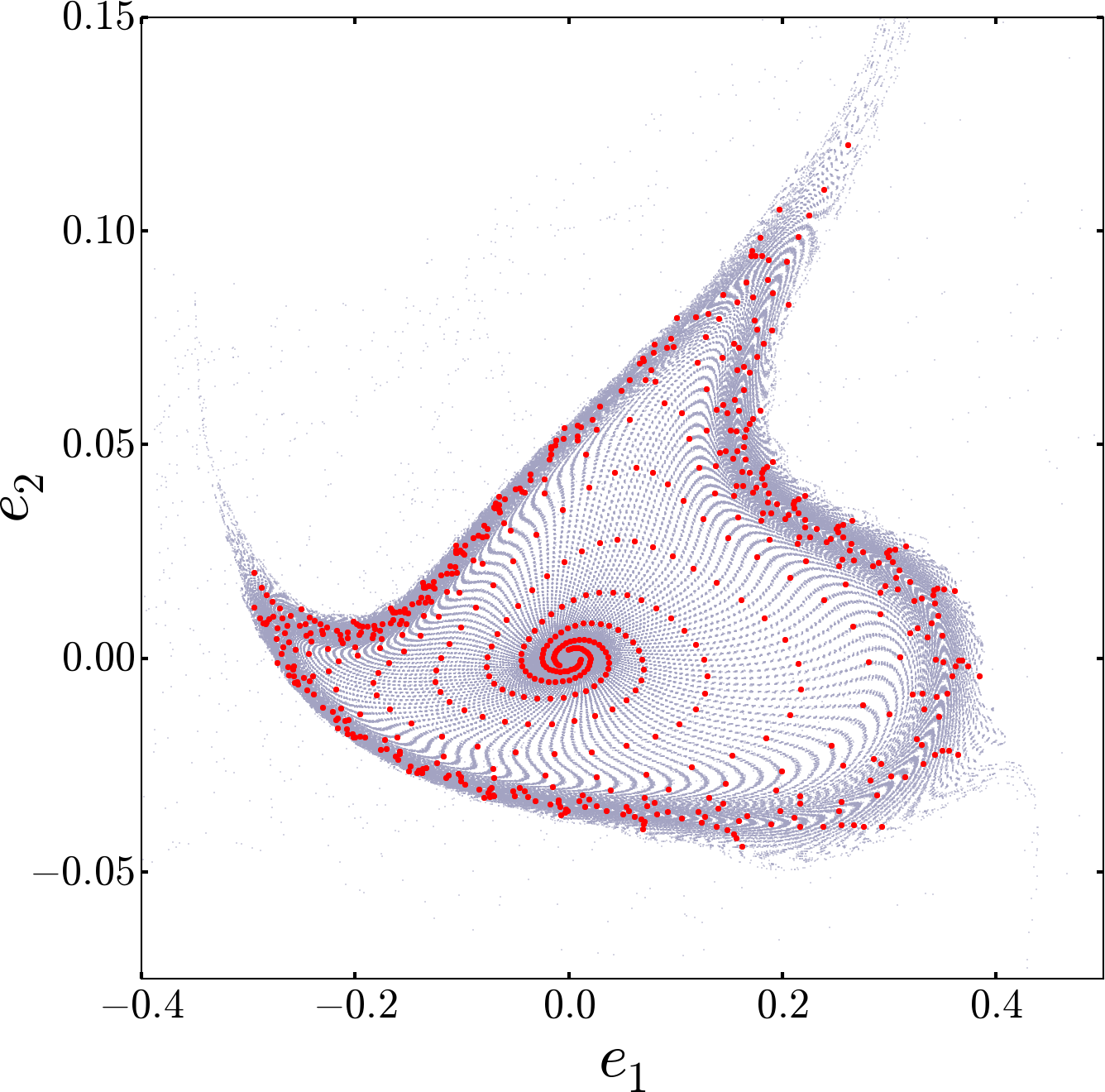
Figure 4: Unstable manifold (gray) of $p_{0}$ on the Poincaré section (18) and an individual trajectory (red) within, system size $L=21.30$.

Assume that $\delta\tilde{a}(0)$ is a small perturbation to $\tilde{a}_{p_{0}}$ that lies in the plane spanned by $({\rm Re}\,[\tilde{V}_{1}],\,{\rm Im}\,[\tilde{V}_{1}])$. Then there exists a coefficient vector $c=(c_{1},c_{2})^{T}$, with which we can express $\delta\tilde{a}(0)$ in this plane as

$$\delta\tilde{a}(0)=Wc\,,$$ (19)

where $W=[{\rm Re}\,[\tilde{V}_{1}],\,{\rm Im}\,[\tilde{V}_{1}]]$ has real and imaginary parts of the Floquet vector $\tilde{V}_{1}$ on its columns. Without a loss of generality, we can rewrite $c$ as $c=\delta rR(\theta)c^{(1)}$, where $c^{(1)}=(1,0)^{T}$ and $R(\theta)$ is a $[2\!\times\!2]$ rotation matrix. Thus (19) can be expressed as $\delta\tilde{a}(0)=\delta rWR(\theta)c^{(1)}$. In the linear approximation, discrete time dynamics $\delta\tilde{a}(n{T_{p_{0}}})$ is given by

$$\delta\tilde{a}(n{T_{p_{0}}})=|\Lambda_{1}|^{n}\delta rWR(\theta-n\arg\Lambda_{1})c^{(1)}\,,$$ (20)

which can then be projected onto the Poincaré section (18) by acting from the left with the projection operator

$$\mathbb{P}(\tilde{a}_{{\cal P}})={\bf 1}-\frac{\tilde{v}(\tilde{a}_{{\cal P}})\otimes\tilde{v}(\tilde{a}_{p_{0}})}{\langle\tilde{v}(\tilde{a}_{{\cal P}}),\,\tilde{v}(\tilde{a}_{p_{0}})\rangle}\,,$$ (21)

computed at $\tilde{a}_{{\cal P}}=\tilde{a}_{p_{0}}$. In (21), $\otimes$ denotes the outer product. Defining $\delta\tilde{a}_{{\cal P}}\equiv\mathbb{P}(\tilde{a}_{{\cal P}})\delta\tilde{a}$ for a small perturbation $\delta\tilde{a}$ to the point $\tilde{a}_{{\cal P}}$ on the Poincaré section, discrete time dynamics of $\delta\tilde{a}_{{\cal P}}$ in the Poincaré section is given by

$$\delta\tilde{a}_{{\cal P}}[n]=|\Lambda_{1}|^{n}\delta rW_{{\cal P}}R(\theta-n\arg\Lambda_{1})c^{(1)}\,,$$ (22)

where $W_{{\cal P}}=[{\rm Re}\,[\tilde{V}_{1,{\cal P}}],\,{\rm Im}\,[\tilde{V}_{1,{\cal P}}]]=\mathbb{P}(\tilde{a}_{p_{0}})W$, and $n$ is the discrete time variable counting returns to the Poincaré section. In the Poincaré section, the solutions (22) define ellipses which expand and rotate respectively by factors of $|\Lambda_{1}|$ and $\arg\Lambda_{1}$ at each return. In order to resolve the unstable manifold, we start trajectories on an elliptic band parameterized by $(\delta,\phi)$, such that the starting point in the band comes to the end of it on the first return, hence totality of these points cover the unstable manifold in the linear approximation. Such set of perturbations are given by

$$\delta\tilde{a}_{{\cal P}}(\delta,\phi)=\epsilon|\Lambda_{1}|^{\delta}W_{{\cal P}}R(\phi)c^{(1)}\,,\quad\mbox{where }\delta\in[0,1)\,,\,\phi\in[0,2\pi)\,,$$ (23)

and $\epsilon$ is a small number. We set $\epsilon=10^{-3}$ and discretize (23) by taking $12$ equidistant points in $[0,1)$ for $\delta$ and $36$ equidistant points in $[0,2\pi)$ for $\phi$ and integrate each $\tilde{a}_{p_{0}}+\delta\tilde{a}_{{\cal P}}(\delta,\phi)$ forward in time. Fig. 4 shows the unstable manifold of $p_{0}$ resolved by this procedure at system size $L=21.30$, for which the torus surrounding $p_{0}$ appears to be unstable as the points approaching to it first slow down and then leave the neighborhood in transverse direction. In order to illustrate this better, we marked an individual trajectory in fig. 4 color red. In fig. 5 we show initial points that go into the calculation, and their first three returns in order to illustrate the principle of the method.

[capbesideposition=left,center,capbesidewidth=0.3]figure[] \begin{overpic}[width=260.17464pt]{UnstMan21p31ret3Zoompng} \put(16.0,12.0){\includegraphics[height=121.41306pt]{UnstMan21p31ret3png}} \end{overpic}

Figure 5: Initial points (black) on the Poincaré section for unstable manifold computation and their first (red), second (green), and third (blue) returns. Inset: zoomed out view of the initial points and their first three returns.

As we continue increasing the system size, we find that at $L\approx 21.36$, trace of the invariant torus disappears and two new periodic orbits $p_{1}$ and $p_{2}$ emerge in the neighborhood of $p_{0}$. Both of these orbits appear as period 3 periodic orbits in the Poincaré map. While $p_{1}$ is unstable (found by a Newton search), $p_{2}$ is initially stable with a finite basin of attraction. The unstable manifold of $p_{0}$ connects heteroclinically to the stable manifolds of $p_{1}$ and $p_{2}$. As we show in fig. 6, resolving the unstable manifold of $p_{0}$ enables us to locate these heteroclinic connections between periodic orbits. Note that 1-dimensional stable manifold of $p_{1}$ separates the unstable manifold of $p_{0}$ in two pieces. Green and blue orbits in fig. 6 appear to be at two sides of this invariant boundary: while one of them converges to $p_{2}$, the other leaves the neighborhood to explore other parts of the state space that are not captured by the Poincaré section, following the unstable manifold of $p_{1}$.

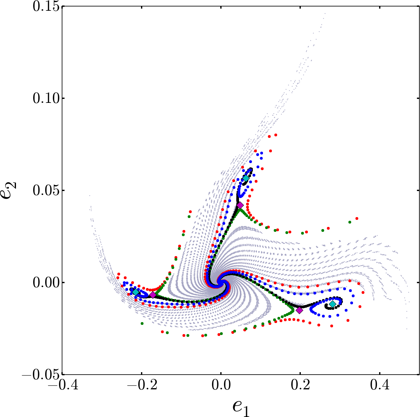
Figure 6: Unstable manifold (gray) of $p_{0}$ on the Poincaré section (18) at $L=21.36$. Colored dots correspond to different individual trajectories within the unstable manifold, with qualitatively different properties. Diamond shaped markers correspond to the period-3 orbits $p_{1}$ (magenta) and $p_{2}$ (cyan).

As the system size is increased, $p_{2}$ becomes unstable at $L\approx 21.38$. At $L\approx 21.477$ the two complex unstable Floquet multipliers collide on the real axis and at $L\approx 21.479$ one of them crosses the unit circle. After this bifurcation, we were no longer able to continue this orbit. At $L=21.48$, the spreading of the $p_{0}$’s unstable manifold becomes more dramatic, and its boundary is set by the 1-dimensional unstable manifold of $p_{1}$, as shown in fig. 7. We compute the unstable manifold of $p_{1}$ similarly to (23), by integrating

$$\tilde{a}_{{\cal P}}(\delta)=\tilde{a}_{p_{1},{\cal P}}\pm\epsilon\Lambda_{1}^{\delta}\tilde{V}_{1,{\cal P}}\,,\quad\mbox{where }\delta\in[0,1)\,.$$ (24)

$\Lambda_{1}$ and $\tilde{V}_{1}$ in (24) are the unstable Floquet multiplier and the corresponding Floquet vector of $\tilde{a}_{p_{1}}$, and the initial conditions (24) cover the unstable manifold of $\tilde{a}_{p_{1}}$ in the linear approximation.

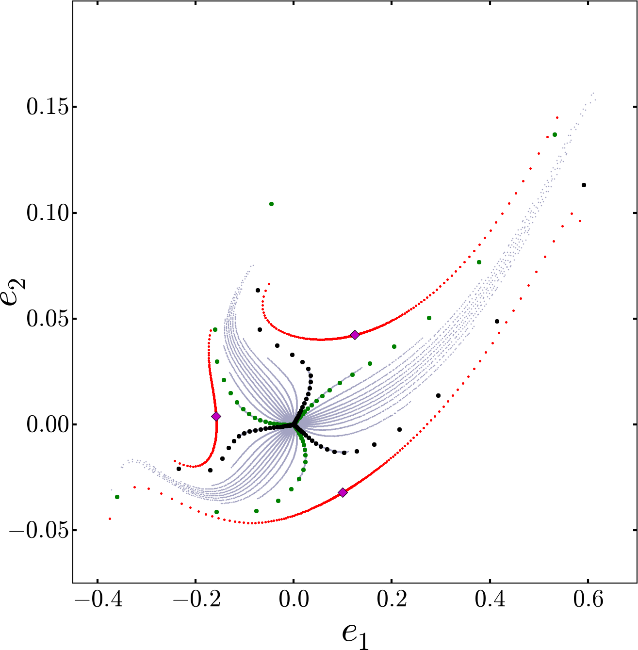
Figure 7: Unstable manifold of $p_{0}$ (gray) and two orbits (black and green) within at $L=21.48$. Red points lie on the 1-dimensional unstable manifold of $p_{1}$ (magenta).

A negative real Floquet multiplier of $p_{1}$ crosses the unit circle at $L\approx 21.6$ leading to “drifting” dynamics in the associated unstable direction. Such “symmetry-breaking” bifurcations of relative periodic orbits with $\textrm{C}_{2}$ symmetry are ubiquitous in many physical settings: Earlier examples are studies of reduced-order models of convection KnoWei81 , forced pendulum DBHL82 , and Duffing oscillator NoFre82 , which reported that symmetry breaking bifurcations precede period doubling route to chaos. A key observation was made by Swift and Wiesenfeld SwiWie84 , who showed in the context of periodically driven damped pendulum that Poincaré map associated with the symmetric system is the second iterate of another “reduced” Poincaré map, which identifies symmetry-equivalent points. They then argue that $\textrm{C}_{2}$-symmetric periodic orbits generically do not undergo period doubling bifurcations when a single parameter of the system varied. More recent works MarLopBla04 ; BlMaLo05 adapt ref. SwiWie84 ’s reduced Poincaré map to fluid systems in order to study their bifurcations in the presence of symmetries. For a review of the symmetry-breaking bifurcations in fluid dynamics, see ref. CraKno91 .

As in the previous cases, in order to investigate the dynamics of the system at this stage, we compute and visualize the unstable manifold of $p_{1}$.

Similarly to (23) and (24), the 2-dimensional unstable manifold of $p_{1}$ is approximately covered by initial conditions

$$\tilde{a}_{{\cal P}}(\delta,\phi)=\tilde{a}_{p_{1},{\cal P}}+\epsilon\left[|\Lambda_{1}|^{\delta}\cos\phi\,\tilde{V}_{1,{\cal P}}+|\Lambda_{2}|^{\delta}\sin\phi\,\tilde{V}_{2,{\cal P}}\right]$$ (25)

where $\delta\in[0,1)\,,\;\phi\in[0,2\pi)$. At system size $L=21.7$, we set $\epsilon=10^{-3}$ and discretize (25) by choosing $10$ and $36$ equally spaced values for $\delta$ and $\phi$, respectively. First $38$ returns of orbits generated according to (25) are shown in fig. 8 as red points along with the unstable manifold of $p_{0}$ (gray). Note that, unlike fig. 7, in fig. 8 there is no clear separation on the unstable manifold of $p_{0}$. This is because the connection of $p_{0}$’s unstable manifold to $p_{1}$ is no longer captured by the Poincaré section (18) after the unstable manifold of $p_{1}$ becomes 2-dimensional. Yet, unstable manifold of $p_{1}$ still shapes that of $p_{0}$.

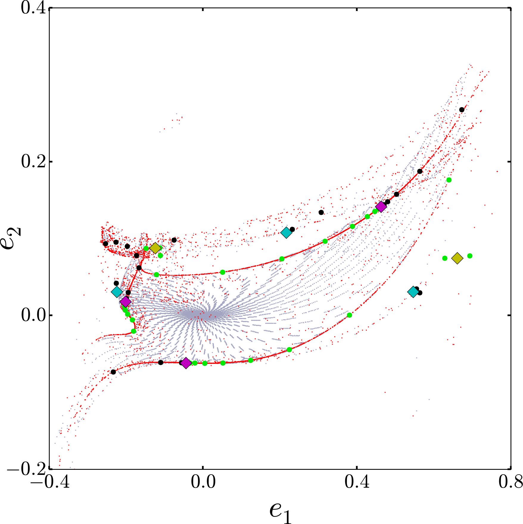
Figure 8: Unstable manifolds of $p_{0}$ (gray) and $p_{1}$ (red) on the Poincaré section (18) at $L=21.7$. Magenta, cyan, and yellow diamond markers respectively indicate the Poincaré section points of $p_{1}$, $p_{3}$, and $p_{4}$. Green and black dots correspond to two individual orbits started on the linear approximation to the unstable manifold of $p_{1}$, which visit neighborhoods of $p_{3}$ and $p_{4}$ respectively.

Since the leading Floquet exponent $\mu_{1}$ of $p_{1}$ is approximately an order of magnitude larger than $\mu_{2}$ (see table 1), unstable manifold of $p_{1}$ appears as if it is 1-dimensional in fig. 8. However, it is absolutely crucial to study this manifold in $2$ dimensions as different initial conditions in this 2-dimensional manifold connect to the regions of state space with qualitatively different dynamics. In order to illustrate this point, we have marked two individual trajectories on the unstable manifold of $p_{1}$ with black and green in fig. 8. After observing that these orbits have nearly recurrent dynamics, we ran Newton searches in their vicinity and found two new periodic orbits $p_{3}$ and $p_{4}$, marked respectively with cyan and yellow diamonds on fig. 8. In the full state space $p_{3}$ is a pre-periodic orbit (9), whereas $p_{4}$ is a relative periodic orbit (7) with a non-zero drift. We show a time segment of the orbit marked green on fig. 8 without symmetry reduction, as color-coded amplitude of the scalar field $u(x,\tau)$ in fig. 9 (a). For comparison we also show two repeats of $p_{1}$ (bottom) and $p_{4}$ (top) in fig. 9 (b). Fig. 9 suggests that this orbit leaves the neighborhood of $p_{1}$ following a heteroclinic connection to $p_{4}$.

[capbesideposition=left,center,capbesidewidth=0.4]figure[] \begin{overpic}[height=195.12767pt]{KSHetCon21p7conf} \put(0.5,-1.0){(a)} \end{overpic}  \begin{overpic}[height=195.12767pt]{KSHetCon21p7POsconf} \put(0.5,-1.0){(b)} \end{overpic}

Figure 9: (a) Space-time visualization of a segment of the orbit marked green on fig. 8 as it leaves the neighborhood of $p_{1}$ and enters the neighborhood of $p_{4}$. (b) Space-time visualizations of $p_{1}$ (bottom) and $p_{4}$ (top).

In fig. 8, some of the red points appear on the unstable manifold of $p_{0}$. These points corresponds to trajectories that leave the unstable manifold of $p_{1}$, come back after exploring other parts of the state space and follow unstable manifold of $p_{0}$. We could have excluded these points by showing shorter trajectories for higher values of $\delta$ in (25) in fig. 8, however we chose not to do so in order to stress that visualizations of unstable manifolds of periodic orbits are not restricted to the dynamics within a small neighborhood of a periodic orbit, but in fact they illuminate the geometry of the flow in a finite part of the strange attractor.

An interesting feature of the bifurcation scenario studied here is the apparent destabilization of the invariant torus before its breakdown. Note that in fig. 4 the trajectories within the unstable manifold of $p_{0}$ diverge in normal direction from the region that was inhabited by a stable 2-torus for lower values of $L$. This suggest that the invariant torus has become normally hyperbolic Feniche71 . This torus could be computed by the method of ref. LCC06 , but our goal here is more modest, what we have computed already amply demonstrates the utility of our $\textrm{O}(2)$ symmetry reduction. Note also that the stable period-3 orbit $p_{2}$ in fig. 6 has a finite basin of attraction, and the trajectories which do not fall into it leave its neighborhood. In typical scenarios involving generation of stable - unstable pairs of periodic orbits within an invariant torus (see e.g. ref. arnold82 ), the torus becomes a heteroclinic connection between the periodic orbit pair. Here the birth of the period-3 orbits appears to destroy the torus.

5 Summary and future directions

The two main results presented here are: 1) a new method for reducing the $\textrm{O}(2)$-symmetry of PDEs, and 2) a symmetry-reduced state space Poincaré  section visualization of 1- and 2-dimensional unstable manifolds of Kuramoto-Sivashinsky periodic orbits.

Our method for the computation of unstable manifolds is general and can find applications in many other ODE and PDE settings. The main idea here is a generalization of Gibson et al. GHCW07 method for visualizations of the unstable manifolds of equilibria, originally applied to plane Couette flow, a setting much more complex then the current paper. All our computations are carried out for the full Kuramoto-Sivashinsky equation (1), in 30 dimensions, and it is remarkable how much information is captured by the 2- and 3-dimensional projections of the $\textrm{O}(2)$ symmetry-reduced Poincaré sections - none of that structure is visible in the full state space.

The Kuramoto-Sivashinsky $\textrm{O}(2)$ symmetry reduction method described here might require modifications when applied to other problems. For example, for PDEs of space dimensions larger then one, there can be more freedom in choosing the phase fixing condition (10). This indeed is the case for shear flows with both homogeneous (streamwise and spanwise translation invariant) and inhomogeneous (wall-normal) directions. When adapting the first Fourier mode slice method to such problems, one should experiment with the dependence of the phase fixing condition on the inhomogeneous coordinate such that the slice fixing phase is uniquely defined for state space regions of interest; see chapter 3 of ref. BudanurThesis for details. Ref. WiShCv15 makes this choice for pipe flow by taking a ‘typical state’ in the turbulent flow, setting all streamwise Fourier modes other than the first one to zero, and using this state as a “slice template”. Another point to be taken into consideration for canonical shear flows is that their symmetry group is $\textrm{SO}(2)\times\textrm{O}(2)$. So far, continuous symmetry reduction in pipe flows ACHKW11 ; WiShCv15 were confined to settings, where an imposed symmetry in conjugacy class of spanwise reflection disallows spanwise rotations. When no such restriction is present, one needs two conditions for fixing both streamwise and spanwise translations. These conditions must be chosen such that the order at which continuous symmetries are reduced does not matter. For direct products of commuting $\textrm{SO}(2)$ symmetries, this is a straightforward task and outlined in section 3 of ref. BudanurThesis . An application of these ideas to the pipe flow is going to appear in a future publication BudHof17 .

Furthermore, while invariant polynomials similar to (16) can be constructed for any problem with a reflection symmetry, an intermediate step is necessary if the action of reflection $\sigma$ symmetry is not the sign flip of a subset of coordinates. In that case, one should first decompose the state space into symmetric and antisymmetric subspaces by computing $a_{S}=(1/2)[a+{D}(\sigma)a]$ and $a_{A}=(1/2)[a-{D}(\sigma)a]$, respectively, and construct invariants analogous to (16) for elements of $a_{A}$ that are not strictly zero. Generalizations of this approach to richer discrete symmetries, such as dihedral groups, remains an open problem, with potential application to systems such as the Kolmogorov flow PlaSirFit91 ; Faraz15 .

Bifurcation scenarios similar to the one studied here are ubiquitous in high-dimensional systems. For example, Avila et al. AvMeRoHo13 study of transition to turbulence in pipe flow, and Zammert and Eckhardt’s study of the plane Poiseuille flow ZamEck15 both report torus bifurcations of relative periodic orbits along transitions to chaos. We believe that the methods presented in this paper can lead to a deeper understanding of these scenarios.

While unstable manifold visualizations of periodic orbits in the symmetry-reduced state space illustrates bifurcations of these orbits, our motivation for investigating such objects is not a study of bifurcations, but ultimately a partition of the turbulent flow’s state space into qualitatively different regions, and construction of the corresponding symbolic dynamics. Fig. 8 and fig. 9 demonstrate our progress in this direction: we are able to identify symmetry breaking heteroclinic connections from non-drifting solutions to the drifting ones. Such observations would have been very hard to make without reducing symmetries of the system, since each relative periodic orbit has a reflection copy, corresponding to a solution drifting in the other direction; and each such solution has infinitely many copies obtained by translations.

Appendix A Computational details

Throughout this paper, we used the $16$ Fourier mode truncation of Kuramoto-Sivashinsky equation (2), which renders the state space $30$-dimensional. Sufficiency of this truncation was demonstrated for $L=22$ in ref. SCD07 . In all our computations, we integrate (12) and its gradient system numerically, using a general purpose adaptive integrator odeint from scipy.integrate scipy , which is a wrapper of lsoda from ODEPACK library hindmarsh1983 . Note that (12) is singular if $\hat{b}_{1}=0$, i.e., whenever the first Fourier mode vanishes. This singularity can be regularized by a time-rescaling if a fixed time step integrator is desired BudCvi14 .

Transformation of trajectories and tangent vectors to the fully symmetry-reduced state space (17) is applied as post-processing. For a trajectory $\hat{a}(\tau)$, we simply apply the reflection reducing transformation to obtain the trajectory as $\tilde{a}(\tau)=\tilde{a}(\hat{a}(\tau))$. Velocity field (12) transforms to (17) by acting with the Jacobian matrix

$$\tilde{v}(\tilde{a})=\frac{d\tilde{a}(\hat{a})}{d\hat{a}}\hat{v}(\hat{a})\,.$$

Floquet vectors transform to the fully symmetry-reduced state space similarly, however, their computations in the first Fourier mode slice requires some care. Remember that the reflection symmetry remains after the continuous symmetry reduction, and its action is represented by (13). Thus, denoting finite time flow induced by (12) by ${\hat{f}^{\tau}(\hat{a})}$, pre-periodic orbit  within the slice satisfies

$$\hat{a}_{pp}=\hat{{D}}(\sigma){\hat{f}^{{T_{p}}}(\hat{a}_{pp})}\,,$$

with its linear stability given by the spectrum of the Jacobian matrix

$$\hat{J}_{\!{}_{pp}}=\hat{{D}}(\sigma)\hat{J}^{{T_{p}}}(\hat{a}_{pp})\,,$$

where $\hat{J}^{{T_{p}}}(\hat{a}_{pp})$ is the Jacobian matrix of the flow function ${\hat{f}^{{T_{p}}}(\hat{a}_{pp})}$. Thus, in order to find the Floquet vectors in fully symmetry-reduced representation, we first find the eigenvectors $\hat{V}$ of the Jacobian matrix $\hat{J}_{\!{}_{pp}}$ and then transform them as $\tilde{V}(\tilde{a})={d\tilde{a}(\hat{a}_{pp})}/{d\hat{a}}\,\hat{V}(\hat{a})\,.$

References

- (1) L. Kadanoff, C. Tang, Proc. Natl. Acad. Sci. USA 81, 1276 (1984). DOI 10.1073/pnas.81.4.1276
- (2) S. Toh, T. Itano, J. Fluid Mech. 481, 67 (2003)
- (3) J.D. Skufca, J.A. Yorke, B. Eckhardt, Phys. Rev. Lett. 96, 174101 (2006). DOI 10.1103/PhysRevLett.96.174101
- (4) T.M. Schneider, B. Eckhardt, J. Yorke, Phys. Rev. Lett. 99, 034502 (2007). DOI 10.1103/PhysRevLett.99.034502
- (5) Y. Duguet, A.P. Willis, R.R. Kerswell, J. Fluid Mech. 613, 255 (2008). DOI 10.1017/S0022112008003248
- (6) M. Avila, F. Mellibovsky, N. Roland, B. Hof, Phys. Rev. Lett. 110, 224502 (2013). DOI 10.1103/PhysRevLett.110.224502
- (7) J.F. Gibson, J. Halcrow, P. Cvitanović, J. Fluid Mech. 611, 107 (2008). DOI 10.1017/S002211200800267X
- (8) J.F. Gibson, Channelflow: A spectral Navier-Stokes simulator in C++. Tech. rep., U. New Hampshire (2013). URL http://Channelflow.org. Channelflow.org
- (9) A.P. Willis, Openpipeflow: Pipe flow code for incompressible flow. Tech. rep., U. Sheffield (2014). URL http://Openpipeflow.org. Openpipeflow.org
- (10) R. Bowen, Equilibrium States and the Ergodic Theory of Anosov Diffeomorphisms (Springer, Berlin, 1975)
- (11) P. Cvitanović, R. Artuso, R. Mainieri, G. Tanner, G. Vattay, Chaos: Classical and Quantum (Niels Bohr Inst., Copenhagen, 2016). URL http://ChaosBook.org
- (12) S. Smale, Bull. Amer. Math. Soc. 73, 747 (1967). DOI 10.1090/S0002-9904-1967-11798-1
- (13) M.C. Gutzwiller, J. Math. Phys. 12, 343 (1971). DOI 10.1063/1.1665596
- (14) D. Ruelle, Bull. Amer. Math. Soc 82, 153 (1976)
- (15) D. Ruelle, Inv. Math. 34, 231 (1976). DOI 10.1007/BF01403069
- (16) P. Cvitanović, Phys. Rev. Lett. 61, 2729 (1988). DOI 10.1103/PhysRevLett.61.2729
- (17) R. Artuso, E. Aurell, P. Cvitanović, Nonlinearity 3, 325 (1990). DOI 10.1088/0951-7715/3/2/005
- (18) R. Artuso, E. Aurell, P. Cvitanović, Nonlinearity 3, 361 (1990). DOI 10.1088/0951-7715/3/2/006
- (19) R. Mainieri, P. Cvitanović, in Chaos: Classical and Quantum (Niels Bohr Inst., Copenhagen, 2016). URL http://ChaosBook.org/paper.shtml#appendHist
- (20) F. Christiansen, P. Cvitanović, V. Putkaradze, Nonlinearity 10, 55 (1997). DOI 10.1088/0951-7715/10/1/004
- (21) Y. Kuramoto, T. Tsuzuki, Progr. Theor. Phys. 55, 356 (1976). DOI 10.1143/PTP.55.356
- (22) G.I. Sivashinsky, Acta Astronaut. 4, 1177 (1977). DOI 10.1016/0094-5765(77)90096-0
- (23) P. Holmes, J.L. Lumley, G. Berkooz, Turbulence, Coherent Structures, Dynamical Systems and Symmetry (Cambridge Univ. Press, Cambridge, 1996)
- (24) P. Cvitanović, R.L. Davidchack, E. Siminos, SIAM J. Appl. Dyn. Syst. 9, 1 (2010). DOI 10.1137/070705623. URL http://arXiv.org/abs/0709.2944
- (25) E.L. Rempel, A.C. Chian, E.E. Macau, R.R. Rosa, Chaos 14, 545 (2004). DOI 10.1063/1.1759297
- (26) E.L. Rempel, A.C. Chian, Phys. Rev. E 71, 016203 (2005). DOI 10.1103/PhysRevE.71.016203
- (27) Y. Lan, P. Cvitanović, Phys. Rev. E 78, 026208 (2008). DOI 10.1103/PhysRevE.78.026208. URL http://arxiv.org/abs/0804.2474
- (28) E.L. Rempel, A.C. Chian, R.A. Miranda, Phys. Rev. E 76, 056217 (2007). DOI 10.1103/PhysRevE.76.056217
- (29) J.M. Greene, J.S. Kim, Physica D 33, 99 (1988). DOI 10.1016/S0167-2789(98)90013-6
- (30) D. Armbruster, J. Guckenheimer, P. Holmes, SIAM J. Appl. Math. 49, 676 (1989). DOI 10.1137/0149039
- (31) I.G. Kevrekidis, B. Nicolaenko, J.C. Scovel, SIAM J. Appl. Math. 50, 760 (1990). DOI 10.1137/0150045
- (32) R.F. Williams, Publ. Math. IHES 50, 73 (1979). DOI 10.1007/BF02684770
- (33) E. Hopf, Bereich. Sächs. Acad. Wiss. Leipzig, Math. Phys. Kl. 94, 19 (1942)
- (34) J. Neimark, Dokl. Akad. Nauk SSSR 129, 736 (1959). In Russian
- (35) R.J. Sacker, Commun. Pure Appl. Math. 18, 717 (1965). DOI 10.1002/cpa.3160180409
- (36) E. Cartan, La méthode du repère mobile, la théorie des groupes continus, et les espaces généralisés, Exposés de Géométrie, vol. 5 (Hermann, Paris, 1935)
- (37) M.J. Field, Trans. Amer. Math. Soc. 259, 185 (1980). DOI 10.1090/S0002-9947-1980-0561832-4
- (38) M. Krupa, SIAM J. Math. Anal. 21, 1453 (1990). DOI 10.1137/0521081
- (39) N.B. Budanur, P. Cvitanović, R.L. Davidchack, E. Siminos, Phys. Rev. Lett. 114, 084102 (2015). DOI 10.1103/PhysRevLett.114.084102
- (40) K. Gatermann, Computer Algebra Methods for Equivariant Dynamical Systems (Springer, New York, 2000)
- (41) P. Chossat, R. Lauterbach, Methods in Equivariant Bifurcations and Dynamical Systems (World Scientific, Singapore, 2000)
- (42) D. Hilbert, Math. Ann. 42, 313 (1893). DOI 10.1007/BF01444162
- (43) E. Noether, Math. Ann. 77, 89 (1915). DOI 10.1007/BF01456821
- (44) R. Gilmore, C. Letellier, The Symmetry of Chaos (Oxford Univ. Press, Oxford, 2007)
- (45) E. Siminos, P. Cvitanović, Physica D 240, 187 (2011). DOI 10.1016/j.physd.2010.07.010
- (46) N.B. Budanur, D. Borrero-Echeverry, P. Cvitanović, Chaos 25, 073112 (2015). DOI 10.1063/1.4923742
- (47) E. Siminos, Recurrent spatio-temporal structures in presence of continuous symmetries. Ph.D. thesis, School of Physics, Georgia Inst. of Technology, Atlanta (2009). URL http://ChaosBook.org/projects/theses.html
- (48) A.P. Willis, P. Cvitanović, M. Avila, J. Fluid Mech. 721, 514 (2013). DOI 10.1017/jfm.2013.75
- (49) R. Miranda, E. Stone, Phys. Lett. A 178, 105 (1993). DOI 10.1016/0375-9601(93)90735-I
- (50) P. Cvitanović, D. Borrero-Echeverry, K. Carroll, B. Robbins, E. Siminos, Chaos 22, 047506 (2012). DOI 10.1063/1.4758309
- (51) E. Knobloch, N. Weiss, Phys. Let. A 85, 127 (1981). DOI 10.1016/0375-9601(81)90882-3
- (52) D. D’Humieres, M.R. Beasley, B.A. Huberman, A. Libchaber, Phys. Rev. A 26, 3483 (1982). DOI 10.1103/PhysRevA.26.3483
- (53) S. Novak, R.G. Frehlich, Phys. Rev. A 26, 3660 (1982). DOI 10.1103/PhysRevA.26.3660
- (54) J.W. Swift, K. Wiesenfeld, Phys. Rev. Lett. 52, 705 (1984). DOI 10.1103/PhysRevLett.52.705
- (55) F. Marques, J.M. Lopez, H.M. Blackburn, Physica D 189, 247 (2004). DOI 10.1016/j.physd.2003.09.041
- (56) H.M. Blackburn, F. Marques, J.M. Lopez, J. Fluid Mech. 522, 395 (2005). DOI 10.1017/S0022112004002095
- (57) J.D. Crawford, E. Knobloch, Ann. Rev. Fluid Mech. 23, 341 (1991). DOI 10.1146/annurev.fl.23.010191.002013
- (58) N. Fenichel, Indiana Univ. Math. J. 21, 193 (1971). DOI 10.1512/iumj.1972.21.21017
- (59) Y. Lan, C. Chandre, P. Cvitanović, Phys. Rev. E 74, 046206 (2006). DOI 10.1103/PhysRevE.74.046206
- (60) V.I. Arnolʹd, Geometrical Methods in the Theory of Ordinary Differential Equations (Springer, Berlin, 1982)
- (61) N.B. Budanur, Exact Coherent Structures in Spatiotemporal Chaos: From Qualitative Description to Quantitative Predictions. Ph.D. thesis, School of Physics, Georgia Inst. of Technology, Atlanta (2015). URL http://ChaosBook.org/projects/theses.html
- (62) A.P. Willis, K.Y. Short, P. Cvitanović, Phys. Rev. E 93, 022204 (2016). DOI 10.1103/PhysRevE.93.022204
- (63) N.B. Budanur, B. Hof. State space geometry of the laminar-turbulent boundary in pipe flow (2017). In preparation
- (64) N. Platt, L. Sirovich, N. Fitzmaurice, Phys. Fluids A 3, 681 (1991). DOI 10.1063/1.858074
- (65) M. Farazmand, J. Fluid M. 795, 278 (2016). DOI 10.1017/jfm.2016.203
- (66) S. Zammert, B. Eckhardt, Phys. Rev. E 91, 041003 (2015). DOI 10.1103/PhysRevE.91.041003
- (67) E. Jones, T. Oliphant, P. Peterson, et al. SciPy: Open source scientific tools for Python (2001). URL http://www.scipy.org
- (68) A.C. Hindmarsh, in Scientific Computing, vol. 1, ed. by R.S. Stepleman (North-Holland, Amsterdam, 1983), pp. 55–64. URL https://computation.llnl.gov/casc/nsde/pubs/u88007.pdf