Abstract

We study the dynamics of a second-order difference equation that is derived from a planar Ricker model of two-stage biological populations. We obtain sufficient conditions for global convergence to zero in the non-autonomous case. This gives general conditions for extinction in the biological context. We also study the dynamics of an autonomous special case of the equation that generates multistable periodic and non-periodic orbits in the positive quadrant of the plane.

1 Introduction

Planar systems of type

$$x_{n+1} =\sigma_{1,n}y_{n}+\sigma_{2,n}x_{n}$$ (1)

$$y_{n+1} =\beta_{n}x_{n}e^{\alpha_{n}-c_{1,n}x_{n}-c_{2,n}y_{n}}$$ (2)

where $\alpha_{n},\beta_{n},\sigma_{i,n},c_{i,n}$ are non-negative numbers for $i=1,2$ and $n\geq 0$ have been used to model single-species, two-stage populations (e.g. juvenile and adult); see [2]–[4], [6] and [11]. The exponential function that defines the time and density dependent fertility rate classifies the above system as a Ricker model. The coefficients $\sigma_{i,n}$ are typically composed of the natural survival rates $s_{i}$ and possibly other factors. For example, they may include harvesting parameters, as in [6] and [11]:

$$\sigma_{i}=(1-h_{i})s_{i},\quad\beta=(1-h_{1})b,\quad c_{1}=(1-h_{1})\gamma,\quad c_{2}=0$$ (3)

All parameters in (3) are assumed to be independent of $n$. In this case, $h_{i},s_{i}\in[0,1]$, $i=1,2$ denote harvest rates and natural survival rates, respectively. The study in [6] shows that the system (1)-(2) under (3) generates a wide range of different behaviors: the occurrence of periodic and chaotic behavior and phenomena such as bubbles and the counter-intuitive “hydra effect” (an increase in harvesting yields an increase in the over-all population) are established for the autonomous system

$$x_{n+1} =(1-h_{1})s_{1}y_{n}+(1-h_{2})s_{2}x_{n}$$

$$y_{n+1} =(1-h_{1})bx_{n}e^{\alpha-(1-h_{1})\gamma x_{n}}.$$

Our results in this paper complement the existing literature, e.g. [1]–[4], [6] and [11]. In the next section we obtain general results on the uniform boundedness and convergence to zero for the non-autonomous system (1)-(2). We also dicuss a refinement of the convergence to zero results when the parameters of the system are periodic (simulating extinction in a periodic environment). In particular, these results show that convergence to zero occurs even if the mean value of $\sigma_{2,n}$ exceeds 1.

In Section 3 we study the dynamics of orbits for a mathematically interesting special case of (1)-(2) in which $\sigma_{2,n}=0.$ This special case was studied with constant parameters (autonomous case) in [3] where conditions for the occurrence of a globally attracting positive fixed point as well as a two-cycle (not globally attracting) were obtained. Conditions implying the occurrence of the two-cycle are of particular interest to us. In this case, the system reduces to a second-order equation with a nonhyperbolic positive fixed point. A semiconjugate factorization of this equation is known (see below) even with variable parameters and we use it to prove the occurrence of complex dynamics, including multiple stable (or multistable) periodic and non-periodic solutions generated from different initial values. Our results also extend the period-two result in [3] to a wider parameter range while allowing some parameters to be periodic.

2 Uniform boundedness and global convergence to zero

For the system (1)-(2) we generally assume that for all $n\geq 0$:

$$\alpha_{n},\beta_{n},\sigma_{i,n},c_{i,n} \geq 0,\quad i=1,2$$ (4)

$$\beta_{n},\sigma_{1,n} >0\ \text{for inifinitely many }n$$

2.1 General results

We begin with a simple, yet useful lemma.

Lemma 1

Let $\alpha>0$, $0<\beta<1$ and $x_{0}\geq 0.$ If for all $n\geq 0$

$$x_{n+1}\leq\alpha+\beta x_{n}$$ (5)

then for every $\varepsilon>0$ and all sufficiently large values of $n$

$$x_{n}\leq\frac{\alpha}{1-\beta}+\varepsilon.$$

Proof. Let $u_{0}=x_{0}$ and note that every solution of the linear, first-order equation $u_{n+1}=\alpha+\beta u_{n}$ converges to its fixed point $\alpha/(1-\beta).$ Further,

$$x_{1} \leq\alpha+\beta x_{0}=\alpha+\beta u_{0}=u_{1}$$

$$x_{2} \leq\alpha+\beta x_{1}\leq\alpha+\beta u_{1}=u_{2}$$

and by induction, $x_{n}\leq u_{n}.$ Since $u_{n}\,\rightarrow\,\alpha/(1-\beta)$ for every $\varepsilon>0$ and all sufficiently large $n$

$$x_{n}\leq u_{n}\leq\frac{\alpha}{1-\beta}+\varepsilon.$$

 

The following result from the literature is quoted as a lemma. See [8] for the proof and some background and references on this result which holds in a more general setting than discussed here.

Lemma 2

Let $\alpha\in(0,1)$ and assume that the functions $f_{n}:[0,\infty)^{k+1}\rightarrow[0,\infty)$ satisfy the inequality

$$f_{n}(u_{0},\ldots,u_{k})\leq\alpha\max\{u_{0},\ldots,u_{k}\}$$ (6)

for all $(u_{0},\ldots,u_{k})\in[0,\infty)$ and all $n\geq 0$. Then for every solution $\{x_{n}\}$ of the difference equation

$$x_{n+1}=f_{n}(x_{n},x_{n-1},\ldots,x_{n-k})$$ (7)

the following is true

$$x_{n}\leq\alpha^{n/(k+1)}\max\{x_{0},x_{-1}\ldots,x_{-k}\}.$$ (8)

Note that (6) implies that $x_{n}=0$ is a constant solution of (7) and further, (8) implies that this solution is globally exponentially stable.

Theorem 3

Assume that (4) holds and further, let $\alpha_{n}$ be bounded and $\limsup_{n\rightarrow\infty}\sigma_{2,n}<1$.

(a) If $\sigma_{1,n}$ is bounded and there is $M>0$ such that $\beta_{n}\leq Mc_{1,n}$ for all $n\geq 0$ then every orbit of (1)-(2) in $[0,\infty)^{2}$ is uniformly bounded.

(b) If $\beta_{n}$ is bounded and the following inequality holds then all orbits of (1)-(2) in $[0,\infty)^{2}$ converge to (0,0):

$$\limsup_{n\rightarrow\infty}\left(\sigma_{1,n}\beta_{n}e^{\alpha_{n}}+\sigma_{2,n}\right)<1.$$ (9)

Proof. (a) For $u,v\geq 0$ and all $n\geq 0$ define

$$\phi_{n}(u,v)=\beta_{n}e^{\alpha_{n}-c_{1,n}u-c_{2,n}v}$$

If $c_{1,n}\not=0$ for all $n$ then elementary calculus yields

$$u\phi_{n}(u,v)\leq u\phi_{n}\left(\frac{1}{c_{1,n}},0\right)=\frac{\beta_{n}}{c_{1,n}}e^{\alpha_{n}-1}$$ (10)

If $c_{1,n}=0$ for some $n$ then $\beta_{n}\leq Mc_{1,n}=0$ and $\phi_{n}(u,v)=0$ for such $n$.

Next, by the hypotheses there are numbers $M_{1},M_{2}>0$ and $\bar{\sigma}\in(0,1)$ such that for all sufficiently large values of $n$

$$\sigma_{1,n}\leq M_{1},\quad\alpha_{n}\leq M_{2},\quad\sigma_{2,n}\leq\bar{\sigma}$$

Since $\beta_{n}\leq Mc_{1,n}$, it follows that for $u,v\geq 0$ and all $n$

$$u\phi_{n}(u,v)\leq Me^{M_{2}-1}\doteq M_{0}$$

It follows that $y_{n}\leq M_{0}$ for $n\geq 1$ so by (1)

$$x_{n+1}\leq M_{0}M_{1}+\sigma_{2,n}(u,v)x_{n}\leq M_{0}M_{1}+\bar{\sigma}x_{n}$$

Next, applying Lemma 1 with $\varepsilon=\bar{\sigma}/(1-\bar{\sigma})$ we obtain for all (large) $n$

$$0\leq x_{n}\leq\frac{M_{0}M_{1}+\bar{\sigma}}{1-\bar{\sigma}}$$

as claimed.

(b) If $\phi_{n}$ is as defined in (a) above then (2) implies that

$$y_{n}\leq\beta_{n}e^{\alpha_{n}}x_{n-1}$$

By (9) there is $\delta\in(0,1)$ such that $\sigma_{1,n}\beta_{n}e^{\alpha_{n}}+\sigma_{2,n}\leq\delta$ for all (large) $n$ so from (1) it follows that

$$x_{n+1} \leq\beta_{n}e^{\alpha_{n}}\sigma_{1,n}x_{n-1}+\sigma_{2,n}x_{n}$$

$$\leq\left(\sigma_{1,n}\beta_{n}e^{\alpha_{n}}+\sigma_{2,n}\right)\max\{x_{n},x_{n-1}\}$$

$$\leq\delta\max\{x_{n},x_{n-1}\}$$

Lemma 2 now implies that $\lim_{n\rightarrow\infty}x_{n}=0.$ Further, since both $\alpha_{n}$ and $\beta_{n}$ are bounded, there is $\mu>0$ such that $\beta_{n}e^{\alpha_{n}}\leq\mu$ for all $n$. Thus,

$$\lim_{n\rightarrow\infty}y_{n}\leq\mu\lim_{n\rightarrow\infty}x_{n-1}=0$$

and the proof is complete.   

Remark 4

1. The hypotheses of the above theorem allow the parameters to contain arbitrary low-level fluctuations, a feature of possible interest in some modeling applications.

2. In Part (a) of the above corollary it is more essential to have $c_{1,n}\not=0$ than $\beta_{n}$ be bounded. Indeed, unbounded solutions occur in the following autonomous linear system

$$x_{n+1} =\sigma_{1}y_{n}+\sigma_{2}x_{n}$$

$$y_{n+1} =\beta e^{\alpha}x_{n}$$

in which $c_{1,n}=0$ for all $n$ and $\beta_{n}=\beta$ is bounded. Note that

$$x_{n+2}=\sigma_{1}y_{n+1}+\sigma_{2}x_{n+1}=\beta e^{\alpha}\sigma_{1}x_{n}+\sigma_{2}x_{n+1}$$

It is evident that unbounded solutions exist unless $\sigma_{1}\beta e^{\alpha}\leq 1-\sigma_{2}$. This is a severe restriction resembling that in Part (b) of the above corollary.

2.2 Global convergence to zero with periodic parameters

Theorem 3 gives general sufficient conditions for the convergence of all non-negative orbits of the planar system to (0,0). In this section we assume that all parameters are periodic and study convergence to zero in this more restricted setting. In particular, the results in this section indicate that global convergence to zero may occur even if (9) does not hold; see Section 2.3 below. Recall from the proof of Theorem 3 that

$$x_{n+1}\leq\beta_{n}e^{\alpha_{n}}\sigma_{1,n}x_{n-1}+\sigma_{2,n}x_{n}.$$ (11)

The right hand side of the above inequality is a linear expression. Consider the linear difference equation

$$u_{n+1}=a_{n}u_{n}+b_{n}u_{n-1},\qquad a_{n+p_{1}}=a_{n},\ b_{n+p_{2}}=b_{n}$$ (12)

where the sequences $a_{n},b_{n}$ have periods $p_{1},p_{2}$ that are positive integers. If $p=\operatorname{lcm}(p_{1},p_{2})$ is the least common multiple of the two periods, we say that the linear difference equation (12) is periodic with period $p.$ We assume that

$$a_{n},b_{n}\geq 0,\quad n=0,1,2,\ldots$$ (13)

In the biological setting, these parameters are defined as follows:

$$a_{n}=\sigma_{2,n},\quad b_{n}=\beta_{n}e^{\alpha_{n}}\sigma_{1,n}$$ (14)

Of interest is the fact that the biological parameters $\alpha_{n},\beta_{n},\sigma_{1,n}$ need not be periodic in order for $a_{n},b_{n}$ to be periodic. As long as the combination of parameters $\beta_{n}e^{\alpha_{n}}\sigma_{1,n}$ is periodic along with $\sigma_{2,n}$ we obtain periodicity. This allows greater flexibility in defining some of the system parameters.

By Lemma 2 every solution of (12) converges to zero if $a_{n}+b_{n}<1$ for all $n.$ However, it is known that convergence to zero may occur even when $a_{n}+b_{n}$ exceeds 1 (for infinitely many $n$ in the periodic case). We use the approach in [9] to examine the consequences of this issue when the planar system has periodic parameters. The following result is an immediate consequence of Theorem 13 in [9].

Lemma 5

Assume that (12) has period $p\geq 1$ and $\delta_{j},\theta_{j}$ for $j=1,2,\ldots,p$ are obtained by iteration from the real initial values

$$\delta_{0}=0,\ \delta_{1}=1;\quad\theta_{0}=1,\ \theta_{1}=0$$ (15)

Suppose that the quadratic polynomial

$$\delta_{p}r^{2}+(\theta_{p}-\delta_{p+1})r-\theta_{p+1}=0$$ (16)

is proper, i.e. not $0=0$ and has a real root $r_{1}\not=0.$ If the recurrence

$$r_{n+1}=a_{n}+\frac{b_{n}}{r_{n}}$$ (17)

generates nonzero real numbers $r_{2},\ldots,r_{p}$ then $\{r_{n}\}_{n=1}^{\infty}$ is periodic with preiod $p$ and yields a semiconjuagte factorization of (12) into a pair of first order equations as follows:

$$t_{n+1} =-\frac{b_{n}}{r_{n}}t_{n},\quad t_{1}=u_{1}-r_{1}u_{0}$$ (18)

$$u_{n+1} =r_{n+1}u_{n}+t_{n+1}.$$ (19)

For an introduction to the concept of semiconjuagte factorization see [7] which also contains the application of this method to linear equations over algebraic fields. A more general application of semiconjugate factorization to linear equations in rings appeares in [9].

The sequence $\{r_{n}\}$ that is generated by (17) is said to be an eigensequence of (12). Eigenvalues are constant eigensequences, since if $p=1$ in Lemma 5 then (16) reduces to

$$r^{2}-\delta_{2}r-\theta_{2}=0\quad\text{or\quad}r^{2}-a_{1}r-b_{1}=0$$

The last equation is recognizable as the charateristic polynomial of (12).

Each of the equations (18) and (19) readily yields a solution by iteration as follows

$$t_{n} =t_{1}(-1)^{n-1}\left(\frac{b_{1}b_{2}\cdots b_{n-1}}{r_{1}r_{2}\cdots r_{n-1}}\right),$$ (20)

$$u_{n} =r_{n}r_{n-1}\cdots r_{2}u_{1}+r_{n}r_{n-1}\cdots r_{3}t_{2}+\cdots r_{n}t_{n-1}+t_{n}$$

$$=r_{n}r_{n-1}\cdots r_{2}r_{1}u_{0}+\sum_{i=1}^{n-1}r_{n}r_{n-1}\cdots r_{i+1}t_{i}+t_{n}$$ (21)

Lemma 6

Suppose that the numbers $\delta_{n}$ and $\theta_{n}$ are defined as in Lemma 5, although here we do not assume that (12) is periodic. Then

(a) $\theta_{n}=0$ for all $n\geq 2$ if and only if $b_{1}=0.$

(b) If (13) holds then for all $n\geq 2$

$$\delta_{n} \geq a_{1}a_{2}\cdots a_{n-1},\quad\theta_{n}\geq b_{1}a_{2}\cdots a_{n-1}$$ (22)

$$\delta_{2n-1} \geq b_{2}b_{4}\cdots b_{2n-2},\quad\theta_{2n}\geq b_{1}b_{3}\cdots b_{2n-1}$$ (23)

Proof. (a) Let $b_{1}=0.$ Then $\theta_{2}=b_{1}=0$ and since $\theta_{1}=0$ by definition it follows that $\theta_{3}=0.$ Induction completes the proof that $\theta_{n}=0$ if $n\geq 2.$ The converse is obvious since $b_{1}=\theta_{2}.$

(b) Since $\delta_{2}=a_{1}$ and $\theta_{2}=b_{1}$ the stated inequalities hold for $n=2.$ If (22) is true for some $k\geq 2$ then

$$\delta_{k+1} =a_{k}\delta_{k}+b_{k}\delta_{k-1}\geq a_{k}\delta_{k}\geq a_{1}a_{2}\cdots a_{k-1}a_{k}$$

$$\theta_{k+1} =a_{k}\theta_{k}+b_{k}\theta_{k-1}\geq a_{k}\theta_{k}\geq b_{1}a_{2}\cdots a_{k-1}a_{k}$$

Now, the proof is completed by induction. The proof of (23) is similar since

$$\delta_{3}=a_{2}\delta_{2}+b_{2}\delta_{1}\geq b_{2}\quad\text{and\quad}\theta_{4}=a_{3}\theta_{3}+b_{3}\theta_{2}\geq b_{3}b_{1}$$

and if (23) holds for some $k\geq 2$ then

$$\delta_{2k+1} \geq b_{2k}\delta_{2k-1}\geq b_{2}b_{4}\cdots b_{2k-2}b_{2k}$$

$$\theta_{2k+2} \geq b_{2k+1}\theta_{2k}\geq b_{1}b_{3}\cdots b_{2k-1}b_{2k+1}$$

which establishes the induction step.   

Lemma 7

Assume that (13) holds with $a_{i}>0$ for $i=1,\ldots,p$ and (12) is periodic with period $p\geq 2.$ Then

(a) Equation (12) has a positive eigensequence $\{r_{n}\}$ of period $p.$

(b) If $b_{i}>0$ for $i=1,\ldots,p$ then

$$r_{1}r_{2}\cdots r_{p}=\frac{1}{2}\left(\delta_{p+1}+\theta_{p}+\sqrt{(\delta_{p+1}-\theta_{p})^{2}+4\delta_{p}\theta_{p+1}}\right)$$ (24)

Hence, $r_{1}r_{2}\cdots r_{p}<1$ if

$$\delta_{p}\theta_{p+1}<(1-\delta_{p+1})(1-\theta_{p})$$ (25)

(c) If $b_{i}<1$ for $i=1,\ldots,p$ then $r_{1}r_{2}\cdots r_{p}>b_{1}b_{2}\cdots b_{p}.$

Proof. (a) Lemma 6 shows that $\delta_{i}>0$ for $i=2,\ldots,p+1.$ Now, either (i) $b_{1}>0$ or (ii) $b_{1}=0.$ In case (i), the root $r^{+}$ of the quadratic polynomial (16) is positive since by Lemma 6 $\theta_{p+1}>0$ and thus

$$r^{+}=\frac{\delta_{p+1}-\theta_{p}+\sqrt{(\delta_{p+1}-\theta_{p})^{2}+4\delta_{p}\theta_{p+1}}}{2\delta_{p}}>\frac{\delta_{p+1}-\theta_{p}+\left|\delta_{p+1}-\theta_{p}\right|}{2\delta_{p}}\geq 0.$$

If $r_{1}=r^{+}$ then from (17) $r_{i}=a_{i-1}+b_{i-1}/r_{i-1}\geq a_{i-1}>0$ for $i=2,\ldots,p+1.$ Thus by Lemma 5, (12) has a unitary (in fact, positive) eigensequence of period $p.$ If $b_{1}=0$ then by Lemma 6 $\theta_{p}=\theta_{p+1}=0$ and (16) reduces to

$$\delta_{p}r^{2}-\delta_{p+1}r=0$$

which has a root $r^{+}=\delta_{p+1}/\delta_{p}>0.$ As in the previous case it follows that (12) has a positive eigensequence of period $p.$

(b) To estalish (24), let $r_{1}=r^{+}$ and note that (16) can be written as

$$r_{1}=\frac{\delta_{p+1}r_{1}+\theta_{p+1}}{\delta_{p}r_{1}+\theta_{p}}$$ (26)

Since $\{r_{n}\}$ has period $p$, $r_{p+1}=r_{1}$ so from (17) and the definition of the numbers $\delta_{n}$ and $\theta_{n}$ it follows that

$$a_{p}+\frac{b_{p}}{r_{p}} =r_{p+1}=\frac{\delta_{p+1}r_{1}+\theta_{p+1}}{\delta_{p}r_{1}+\theta_{p}}=\frac{(a_{p}\delta_{p}+b_{p}\delta_{p-1})r_{1}+a_{p}\theta_{p}+b_{p}\theta_{p-1}}{\delta_{p}r_{1}+\theta_{p}}$$

$$=\frac{a_{p}(\delta_{p}r_{1}+\theta_{p})+b_{p}(\delta_{p-1}r_{1}+\theta_{p-1})}{\delta_{p}r_{1}+\theta_{p}}$$

$$=a_{p}+\frac{b_{p}}{(\delta_{p}r_{1}+\theta_{p})/(\delta_{p-1}r_{1}+\theta_{p-1})}$$

Since $b_{p}\not=0$ it follows that

$$r_{p}=\frac{\delta_{p}r_{1}+\theta_{p}}{\delta_{p-1}r_{1}+\theta_{p-1}}$$

We claim that if $b_{i}\not=0$ for $i=1,\ldots,p$ then

$$r_{p-j}=\frac{\delta_{p-j}r_{1}+\theta_{p-j}}{\delta_{p-j-1}r_{1}+\theta_{p-j-1}},\quad j=0,1,\ldots,p-2$$ (27)

This claim is easily seen to be true by induction; we showed that it is true for $j=0$ and if (27) holds for some $j$ then by (17)

$$a_{p-j-1}+\frac{b_{p-j-1}}{r_{p-j-1}} =r_{p-j}=\frac{(a_{p-j-1}\delta_{p-j-1}+b_{p-j-1}\delta_{p-j-2})r_{1}+(a_{p-j-1}\theta_{p-j-1}+b_{p-j-1}\theta_{p-j-2})}{\delta_{p-j-1}r_{1}+\theta_{p-j-1}}$$

$$=\frac{a_{p-j-1}(\delta_{p-j-1}r_{1}+\theta_{p-j-1})+b_{p-j-1}(\delta_{p-j-2}r_{1}+\theta_{p-j-2})}{\delta_{p-j-1}r_{1}+\theta_{p-j-1}}$$

$$=a_{p-j-1}+\frac{b_{p-j-1}(\delta_{p-j-2}r_{1}+\theta_{p-j-2})}{\delta_{p-j-1}r_{1}+\theta_{p-j-1}}$$

from which it follows that

$$r_{p-j-1}=\frac{\delta_{p-j-1}r_{1}+\theta_{p-j-1}}{\delta_{p-j-2}r_{1}+\theta_{p-j-2}}$$

and the induction argument is complete. Now, using (27) we obtain

$$r_{p}r_{p-1}\cdots r_{2}r_{1}=\frac{\delta_{p}r_{1}+\theta_{p}}{\delta_{p-1}r_{1}+\theta_{p-1}}\frac{\delta_{p-1}r_{1}+\theta_{p-1}}{\delta_{p-2}r_{1}+\theta_{p-2}}\cdots\frac{\delta_{2}r_{1}+\theta_{2}}{\delta_{1}r_{1}+\theta_{1}}r_{1}=\delta_{p}r_{1}+\theta_{p}$$ (28)

Given that $r_{1}=r^{+}$ (28) implies that

$$r_{1}r_{2}\cdots r_{p} =\delta_{p}\frac{\delta_{p+1}-\theta_{p}+\sqrt{(\delta_{p+1}-\theta_{p})^{2}+4\delta_{p}\theta_{p+1}}}{2\delta_{p}}+\theta_{p}$$

$$=\frac{1}{2}\left(\delta_{p+1}+\theta_{p}+\sqrt{(\delta_{p+1}-\theta_{p})^{2}+4\delta_{p}\theta_{p+1}}\right)$$

and (24) is obtained. Hence, $r_{1}r_{2}\cdots r_{p}<1$ if

$$\delta_{p+1}+\theta_{p}+\sqrt{(\delta_{p+1}-\theta_{p})^{2}+4\delta_{p}\theta_{p+1}}<2$$

Upon rearranging terms and squaring:

$$(\delta_{p+1}-\theta_{p})^{2}+4\delta_{p}\theta_{p+1}<4-4(\delta_{p+1}+\theta_{p})+(\delta_{p+1}+\theta_{p})^{2}$$

which reduces to (25) after straightforward algebraic manipulations.

(c) First, assume that $p$ is odd. Then by (23)

$$\delta_{p}\theta_{p+1}=(b_{2}b_{4}\cdots b_{p-1})(b_{1}b_{3}\cdots b_{p})=b_{1}b_{2}\cdots b_{p}$$

so from (24)

$$r_{1}r_{2}\cdots r_{p}>\sqrt{\delta_{p}\theta_{p+1}}=\sqrt{b_{1}b_{2}\cdots b_{p}}$$

If $b_{i}<1$ for $i=1,\ldots,p$ then $b_{1}b_{2}\cdots b_{p}<1$ so $\sqrt{b_{1}b_{2}\cdots b_{p}}>b_{1}b_{2}\cdots b_{p}$ as required. Now let $p$ be even. Then from (24) and (23)

$$r_{1}r_{2}\cdots r_{p}>\frac{\delta_{p+1}+\theta_{p}}{2}\geq\frac{b_{2}b_{4}\cdots b_{p}+b_{1}b_{3}\cdots b_{p-1}}{2}$$

If $b_{i}<1$ for $i=1,\ldots,p$ then $b_{2}b_{4}\cdots b_{p}\geq b_{1}b_{2}\cdots b_{p}$ and$\ b_{1}b_{3}\cdots b_{p-1}\geq b_{1}b_{2}\cdots b_{p}$ and the proof is complete.   

Theorem 8

Assume that the sequences $\beta_{n}e^{\alpha_{n}}\sigma_{1,n}$ and $\sigma_{2,n}$ are strictly positive and periodic and let $p$ be the least common multiple of their periods. All non-negative orbits of (1)-(2) converge to (0,0) if $\beta_{i}e^{\alpha_{i}}\sigma_{1,i}<1$ for $i=1,\ldots,p$ and (25) holds.

Proof. Let $\{u_{n}\}$ be a solution of the linear equation (12) with $a_{n},b_{n}$ defined by (14). If $u_{0}=x_{0}$ and $u_{1}=x_{1}$ then by (11)

$$x_{2} \leq\beta_{0}e^{\alpha_{0}}\sigma_{1,1}x_{0}+\sigma_{2,1}x_{1}=\beta_{0}e^{\alpha_{0}}\sigma_{1,1}u_{0}+\sigma_{2,1}u_{1}=u_{2}$$

$$x_{3} \leq\beta_{1}e^{\alpha_{1}}\sigma_{1,2}x_{2}+\sigma_{2,2}x_{2}\leq\beta_{1}e^{\alpha_{1}}\sigma_{1,2}u_{1}+\sigma_{2,2}u_{2}=u_{3}$$

By induction it follows that $x_{n}\leq u_{n}.$ If (25) holds then by Lemma 7, $\lim_{n\rightarrow\infty}u_{n}=0$ so $\{x_{n}\}$ converges to 0. Further, $\lim_{n\rightarrow\infty}y_{n}=0$ as in the proof of Theorem 3 and the proof is complete.   

Recall that the individual sequences $\alpha_{n},\beta_{n},\sigma_{1,n}$ need not be periodic; see the note following (14). Therefore, Theorem 8 applies to the system (1)-(2) even if the system itself is not periodic as long as the combination $\beta_{n}e^{\alpha_{n}}\sigma_{1,n}$ of parameters is periodic along with $\sigma_{2,n}.$

2.3 Stocking strategies that do not prevent extinction

Condition (25) involves the numbers $\delta_{j},\theta_{j}$ rather than the coefficients of (12) directly. To illustrate the biological significance of this condition with regard to extinction, consider the case of period $p=2$ in which the role of $a_{i}$, $b_{i}$ is more apparent. Inequality (25) in this case is

$$\delta_{2}\theta_{3} <(1-\delta_{3})(1-\theta_{2})$$

$$a_{1}a_{2}b_{1} <(1-b_{2}-a_{1}a_{2})(1-b_{1})$$

Simple manipulations reduce the last inequality to

$$a_{1}a_{2}<(1-b_{1})(1-b_{2}).$$ (29)

In this form, it is easy to see the signficance of (25) with regard to extinction. For if $b_{1},b_{2}<1$ then (29) holds even if $a_{1}>1$ or $a_{2}>1$ so global convergence to (0,0) my occur when (9) does not hold. Further, it is possible that (29) holds, together with arbitrarily large mean value

$$\frac{a_{1}+a_{2}}{2}>1$$ (30)

if, say $a_{1}\rightarrow 0$ as $a_{2}\rightarrow\infty$. In population models this implies that if (29) holds with

$$a_{i}=\sigma_{2,i},\quad b_{i}=\beta_{i}e^{\alpha_{i}}\sigma_{1,i}\qquad i=1,2$$

then extinction may still occur after restocking the adult population so that the mean value of the composite parameter $\sigma_{2,n}$ exceeds unity by a wide margin.

3 Complex multistable behavior

In this section we consider the reduced system

$$x_{n+1} =\sigma_{1,n}y_{n}$$ (31)

$$y_{n+1} =\beta_{n}x_{n}e^{\alpha_{n}-c_{1,n}x_{n}-c_{2,n}y_{n}}$$ (32)

where we assume that

$$\sigma_{1,n},c_{1,n},c_{2,n},\beta_{n}>0,\text{\quad}\alpha_{n}\geq 0.$$ (33)

In the context of stage-structured models the assumption $\sigma_{2,n}=0$ applies in particular, to the case of a semelparous species, i.e. an organism that reproduces only once before death. Additional interpretations in terms of harvesting, migrations or other factors may be possible if $\sigma_{2,n}$ includes additional factors beyond the natural adult survival rate.

The system (31)-(32) with $c_{2,n}=0$ has been studied in the literature; for instance, an autonomous version is discussed in [6] and [11]. The assumption $c_{2,n}>0,$ which adds greater inter-species competition into the stage-structured model, leads to theoretical issues that are not well-understood. We proceed by folding he system (31)-(32) to a second-order difference equation. The process here is simple and self-contained but for a broader introduction and other applications of folding to the study of discrete planar systems we refer to [10].

From (31) we obtain $y_{n}=x_{n+1}/\sigma_{1,n}$. Now using (31) and (32) we obtain:

$$x_{n+2}=\sigma_{1,n+1}\beta_{n}x_{n}e^{\alpha_{n}-c_{1,n}x_{n}-c_{2,n}y_{n}}=\sigma_{1,n}\beta_{n}x_{n}e^{\alpha_{n}-c_{1,n}x_{n}-(c_{2,n}/\sigma_{1,n})x_{n+1}}$$

This can be written more succinctly as

$$x_{n+1}=x_{n-1}e^{a_{n}-c_{1,n}x_{n-1}-(c_{2,n}/\sigma_{1,n})x_{n}}$$ (34)

where

$$a_{n}=\alpha_{n}+\ln(\beta_{n}\sigma_{1,n+1}).$$

3.1 Fixed points, global stability

It is useful to start by examining the fixed points of (34) when all parameters are constants, i.e. if (31)-(32) is an autonomous system. Then (34) takes the form of the autonomous difference equation:

$$x_{n+1}=x_{n-1}e^{a-c_{1}x_{n-1}-(c_{2}/\sigma_{1})x_{n}}$$ (35)

This equation clearly has a fixed point at 0. The following is consequence of Theorem 3(b).

Corollary 9

Assume that the system (31)-(32) is autonomous, i.e. $\alpha_{n}=\alpha$, $\beta_{n}=\beta$, $\sigma_{1,n}=\sigma_{1}$, $c_{1,n}=c_{1}$ and $c_{2,n}=c_{2}$ are constants for all $n$.

(a) If $a=\alpha+\ln(\beta\sigma_{1})<0$ then 0 is the unique fixed point of (35) in $[0,\infty)$ and all positive solutions of (35) converge to zero.

(b) The eigenvalues of the linearization of (35) at 0 are $\pm e^{a/2}$; thus, 0 is locally asymptotically stable if $a<0.$

If $a>0$ then (35) has exactly two fixed points: 0 and a positive fixed point

$$\bar{x}=\frac{a\sigma_{1}}{c_{1}\sigma_{1}+c_{2}}.$$

Substituting $r_{n}=c_{1}x_{n}$ in (35) yields

$$r_{n+1}=r_{n-1}e^{a-r_{n-1}-br_{n}},\quad b=\frac{c_{2}}{\sigma_{1}c_{1}}$$ (36)

The positive fixed point of this equation is

$$\bar{r}=\frac{a}{1+b}=c_{1}\bar{x}.$$

The next result is proved in [3].

Theorem 10

Let $a\in(0,1]$.

(a) If $b\in(0,1)$ (i.e. $c_{2}<\sigma_{1}c_{1}$) then the positive fixed point $\bar{r}$ of (36) is a global attractor of all of its positive solutions.

(b) If $b=1$ (i.e. $c_{2}=\sigma_{1}c_{1}$) then every non-constant, positive solution of (36) converges to a 2-cycle whose consecutive points satisfy $r_{n}+r_{n+1}=a,$ i.e. the mean value of the limit cycle is the fixed point $\bar{r}=a/2.$

The two-cycle in Theorem 10(b) is not unique–it is determined by the initial values. We derive the precise mechanism that explains this, and much more complex behavior below. In particular, we extend Part (b) of Theorem 10 by showing that it holds for $a\in(0,2]$ and even some parameters need not be constants.

3.2 Order reduction

The semiconjugate factorization method that we used earlier for linear equations also applies to (34) if the following condition holds:

$$c_{2,n}=\sigma_{1,n}c_{1,n}\quad n=0,1,2,\ldots$$ (37)

In the autonomous case this reduces to the condition in Theorem 10(b), i.e. $c_{2}=\sigma_{1}c_{1}.$ This condition that is restrictive but admissible in a biological sense, leads to interesting nonhypberbolic dynamics that we explore in the remainder of this paper.

If (37) holds then we substitute $r_{n}=c_{1,n}x_{n}$ in (34) to obtain

$$r_{n+1}=\frac{c_{1,n+1}}{c_{1,n-1}}r_{n-1}e^{a_{n}-r_{n-1}-r_{n}}$$

which can be written as

$$r_{n+1} =r_{n-1}e^{d_{n}-r_{n-1}-r_{n}}$$ (38)

$$d_{n} =a_{n}+\ln[c_{1,n+1}/c_{1,n-1}].$$

Note that if $c_{1,n}$ has period 2 or is constant then $c_{1,n+1}=c_{1,n-1}$ so $d_{n}=a_{n}.$ In any case, a solution $x_{n}=r_{n}/c_{1,n}$ of (34) is derived in terms of a solution of (38) when (37) holds.

Equation (38) admits a semiconjugate factorization that splits it into two equations of order one. Using the concept of form symmetry from [7], we define

$$t_{n}=\frac{r_{n}}{r_{n-1}e^{-r_{n-1}}}$$

for each $n\geq 1$ and note that

$$t_{n+1}t_{n}=\frac{r_{n+1}}{r_{n}e^{-r_{n}}}\frac{r_{n}}{r_{n-1}e^{-r_{n-1}}}=\frac{r_{n+1}}{r_{n-1}e^{-r_{n-1}-r_{n}}}=e^{d_{n}}$$

or equivalently,

$$t_{n+1}=\frac{e^{d_{n}}}{t_{n}}.$$ (39)

Now

$$r_{n+1}=e^{d_{n}}r_{n-1}e^{-r_{n-1}}e^{-r_{n}}=e^{d_{n}}\frac{r_{n}}{t_{n}}e^{-r_{n}}=\frac{e^{d_{n}}}{t_{n}}r_{n}e^{-r_{n}}=t_{n+1}r_{n}e^{-r_{n}}$$ (40)

The pair of equations (39) and (40) constitute the semiconjugate factorization of (38):

$$t_{n+1} =\frac{e^{d_{n}}}{t_{n}},\quad t_{0}=\frac{r_{0}}{r_{-1}e^{-r_{-1}}}$$ (41)

$$r_{n+1} =t_{n+1}r_{n}e^{-r_{n}}$$ (42)

Every solution $\{r_{n}\}$ of (38) is generated by a solution of the system (41)-(42). Using the initial values $r_{-1},r_{0}$ we obtain a solution $\{t_{n}\}$ of the first-order equation (41). This solution is then used to obtain a solution of (42), and thus also of (38).

3.3 Complex behavior for the autonomous equation

If $p=1$ then $d_{n}$ is constant, say $d_{n}=d$ for all $n$. In this case (38) reduces to the autonomous equation:

$$r_{n+1}=r_{n-1}e^{d-r_{n-1}-r_{n}}$$ (43)

although (34) may not be autonomous, e.g. if $c_{1,n}$ has period 2, as noted above.

If $d<0$ then Corollary 9 implies that all solutions of (43) converge to 0. Let $d>0$ so that there is a positive fixed point

$$\bar{r}=\frac{d}{2}>0.$$

The eigenvalues of the linearization of (43) at $\bar{r}$ are $-1$ and $-d/2$, showing in particular that $\bar{r}$ is nonhyperbolic. The behavior of solutions of (43) is sufficiently unusual that we use the numerical simulation depicted in Figure 1 to motivate the subsequent discussion.

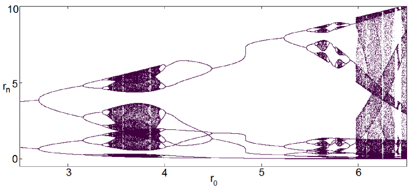
Figure 1: Bifurcation of multiple stable solutions in the state-space

In Figure 1, $d=4.5$, $r_{-1}=d/2=2.25$ is fixed and $r_{0}\in(0,\infty)$ acts as a bifurcation parameter. The changing values of $r_{0}$ are shown on the horizontal axis in the range 2.5 to 6.5. For every grid value of $r_{0}$ in the indicated range, 300 points of the corresponding solution $\{r_{n}\}$ are plotted vertically. In this figure, coexisting solutions with periods 2, 4, 8 and 16 are easily identified. The solutions shown in Figure 1 are stable since they are generated by numerical simulation, so that qualitatively different, stable solutions exist for (43) for different initial values. In the remainder of this section we explain this abundance of multistable solutions for (43) using the reduction (41)-(42).

All solutions of (41) with constant $d_{n}=d$ and $t_{0}\neq e^{d/2}$ are periodic with period 2:

$$\left\{t_{0},\frac{e^{d}}{t_{0}}\right\}=\left\{\frac{r_{0}}{r_{-1}e^{-r_{-1}}},\frac{r_{-1}e^{d-r_{-1}}}{r_{0}}\right\}.$$

Hence the orbit of each nontrivial solution $\{r_{n}\}$ of (43) in its state-space, namely, the $(r_{n},r_{n+1})$-plane, is restricted to the class of curve-pairs

$$g_{0}(r,t_{0})=t_{0}re^{-r}\quad\text{and\quad}g_{1}(r,t_{0})=t_{1}re^{-r},\quad t_{1}=\frac{e^{d}}{t_{0}}$$ (44)

These one-dimensional mappings form the building blocks of the two-dimensional, standard state-space map $F$ of (43), i.e.

$$F(u,r)=(r,ue^{d-u-r}).$$

There are, of course, an infinite number of initial value-dependent curve-pairs for the map $F.$

The next result indicates the specific mechanism for generating the solutions of (43) from its semiconjugate factorization.

Lemma 11

Let $d>0$ and let $\{r_{n}\}$ be a solution of (43) with initial values $r_{-1},r_{0}>0$.

(a) For $k=0,1,2,\ldots$ and $t_{0}$ as defined in (41)

$$r_{2k+1}=g_{1}\circ g_{0}(r_{2k-1},t_{0}),\quad r_{2k+2}=g_{0}\circ g_{1}(r_{2k},t_{0})$$

Thus, the odd terms of every solution of (43) are generated by the class of one-dimensional maps $g_{1}\circ g_{0}$ and the even terms by $g_{0}\circ g_{1}$;

(b) If the initial values  $r_{-1},r_{0}$ satisfy

$$r_{0}=r_{-1}e^{d/2-r_{-1}}$$ (45)

then $g_{0}(r,t_{0})=g_{1}(r,t_{0})=re^{d/2-r}$; i.e. the two curves $g_{0}$ and $g_{1}$ coincide with the curve

$$g(r)\doteq re^{d/2-r}$$

The trace of $g$ contains the fixed point $(\bar{r},\bar{r})$ in the state-space and is invariant under $F.$

Proof. (a) For $k=0,1,2,\ldots$ (42) implies that

$$r_{2k+1} =t_{2k+1}r_{2k}e^{-r_{2k}}=t_{1}r_{2k}e^{-r_{2k}}=g_{1}(r_{2k},t_{0})$$

$$r_{2k} =t_{2k}r_{2k-1}e^{-r_{2k-1}}=t_{0}r_{2k-1}e^{-r_{2k-1}}=g_{0}(r_{2k-1},t_{0})$$

Therefore,

$$r_{2k+1}=g_{1}(g_{0}(r_{2k-1},t_{0}),t_{0})=g_{1}\circ g_{0}(r_{2k-1},t_{0})$$

A similar calculation shows that

$$r_{2k+2}=g_{0}(g_{1}(r_{2k},t_{0}),t_{0})=g_{0}\circ g_{1}(r_{2k},t_{0})$$

and the proof of (a) is complete.

(b) Note that $g(\bar{r})=\bar{r}e^{d/2-\bar{r}}=\bar{r}$ so the trace of $g$ contains $(\bar{r},\bar{r}).$ The curves $g_{0},g_{1}$ coincide if $t_{0}=e^{d}/t_{0}$, i.e. $t_{0}=e^{d/2}.$ This happens if the initial values  $r_{-1},r_{0}$ satisfy (45). In this case, $(r_{-1},r_{0})$ is clearly on the trace of $g$ and by (42)

$$r_{1}=t_{1}r_{0}e^{-r_{0}}=\frac{e^{d}}{t_{0}}r_{0}e^{-r_{0}}=t_{0}r_{0}e^{-r_{0}}=g(r_{0})$$

Therefore, the point $(r_{0},r_{1})$ is also on the trace of $g.$ Since $t_{n}=t_{0}$ for all $n$ if $t_{0}=e^{d/2}$ the same argument applies to $(r_{n},r_{n+1})$ for all $n$ and completes the proof by induction.   

Note that the invariant curve $g$ does not depend on initial values. There is also the following useful fact about $g$.

Lemma 12

The mapping $g$ has a period-three point for $d\geq 6.26.$

Proof. Let $a=d/2.$ The third iterate of $g$ is

$$g^{3}(r)=r\exp(3a-r-2re^{a-r}+e^{a-re^{a-r}})$$

In particular,

$$g^{3}(1)<\exp(3a-1-e^{a-1})\doteq h(a)$$

Solving $h(a)=1$ numerically yields the estimate $a\approx 3.12.$ Since $h(a)$ is decreasing if $a>2.1$ it follows that $h(a)<1$ if $a\geq 3.13$. Therefore, $g^{3}(1)<1$ for $d\geq 6.26.$ Further, for $\varepsilon\in(0,a)$

$$g^{3}(a-\varepsilon) >(a-\varepsilon)\exp\left[2a+\varepsilon-2(a-\varepsilon)e^{\varepsilon}+e^{a(1-e^{\varepsilon})}\right]$$

$$>(a-\varepsilon)\exp[e^{-a(e^{\varepsilon}-1)}-2a(e^{\varepsilon}-1)]$$

For sufficiently small $\varepsilon$ the exponent is positive so we may assert that

$$g^{3}(1)<1<a-\varepsilon<g^{3}(a-\varepsilon)$$

Hence, there is a root of $g^{3}(r)$, or a period-three point of $g$ in the interval $(1,a)$ if $a\geq 3.13$, i.e. $d\geq 6.26$.   

The function compositions in Lemma 11 are specifically the following mappings:

$$g_{1}\circ g_{0}(r,t_{0}) =re^{d-r-t_{0}re^{-r}},$$

$$g_{0}\circ g_{1}(r,t_{0}) =re^{d-r-t_{1}re^{-r}},\quad t_{1}=\frac{e^{d}}{t_{0}}.$$

To simplify our notation, for each $t\in(0,\infty)$ define the class of functions $f_{t}:(0,\infty)\rightarrow(0,\infty)$ as

$$f_{t}(r)=re^{d-r-tre^{-r}}.$$

We also abbreviate $f_{t_{0}}$ as $f_{0}$, $f_{t_{1}}$ as $f_{1}$, $g_{0}(\cdot,t_{0})$ as $g_{0}$ and $g_{1}(\cdot,t_{0})$ as $g_{1}$. Then we see from the preceding discussion that

$$g_{1}\circ g_{0}=f_{0},\quad g_{0}\circ g_{1}=f_{1}.$$ (46)

According to Lemma 11, iterations of $f_{0}$ generate the odd-indexed terms of a solution of (43) and iterations of $f_{1}$ generate the even-indexed terms.

The next result furnishes a relationship between $f_{i}$ and $g_{i}$ for $i=0,1.$

Lemma 13

Let $t_{0}\in(0,\infty)$ be fixed and $t_{1}=e^{d}/t_{0}.$ Then

$$f_{1}\circ g_{0}=g_{0}\circ f_{0}\quad\text{and\quad}f_{0}\circ g_{1}=g_{1}\circ f_{1}.$$ (47)

Proof. This may be established by straightforward calculation using the definitions of the various functions, or alternatively, use (46) to obtain

$$f_{1}\circ g_{0}=\left(g_{0}\circ g_{1}\right)\circ g_{0}=g_{0}\circ(g_{1}\circ g_{0})=g_{0}\circ f_{0}$$

This proves the first equality in (47) and the second equality is proved similarly.   

The equalities in (47) are not conjugacies since $g_{0}$ and $g_{1}$ are not one-to-one. However, the following is implied.

Lemma 14

(a) If $\{s_{1},s_{2},\ldots,s_{q}\}$ is a $q$-cycle of $f_{0},$ i.e. a solution (listed in the order of iteration) of

$$s_{n+1}=f_{0}(s_{n})=s_{n}e^{d-s_{n}-t_{0}s_{n}e^{-s_{n}}}$$ (48)

with minimal (or prime) period $q\geq 1$ then $\{g_{0}(s_{1}),g_{0}(s_{2}),\ldots,g_{0}(s_{q})\}$ is a $q$-cycle of $f_{1},$ i.e. a solution of

$$u_{n+1}=f_{1}(u_{n})=u_{n}e^{d-u_{n}-t_{1}u_{n}e^{-u_{n}}}$$ (49)

with period $q$ (listed in the order of iteration). Similarly, if $\{u_{1},u_{2},\ldots,u_{q}\}$ is a $q$-cycle of $f_{1},$ i.e. a solution of (49) with minimal period $q\geq 1$ then $\{g_{1}(u_{1}),g_{1}(u_{2}),\ldots,g_{1}(u_{q})\}$ is a $q$-cycle of $f_{0},$ i.e. solution of (48) with period $q$.

(b) If $\{s_{n}\}$ is a non-periodic solution of (48) then $\{g_{0}(s$${}_{n})\}$ is a non-periodic solution of (49). Similarly, if $\{u_{n}\}$ is a non-periodic solution of (49) then $\{g_{1}(u_{n})\}$ is a non-periodic solution of (48).

Proof. (a) By the hypothesis, $f_{0}(s_{n+q})=s_{n}$ for all $n$ and in the order of iteration

$$f_{0}(s_{k})=s_{k+1}\quad\text{for }k=1,\ldots,q-1\text{\quad and\quad}f_{0}(s_{q})=s_{1}.$$

By Lemma 13,

$$f_{1}(g_{0}(s_{n+q}))=g_{0}(f_{0}(s_{n+q}))=g_{0}(s_{n})$$

and also

$$f_{1}(g_{0}(s_{k})) =g_{0}(f_{0}(s_{k}))=g_{0}(s_{k+1})\quad\text{for }k=1,\ldots,q-1,$$

$$f_{1}(g_{0}(s_{q})) =g_{0}(f_{0}(s_{q}))=g_{0}(s_{1})$$

It follows that $\{g_{0}(s_{1}),g_{0}(s_{2}),\ldots,g_{0}(s_{q})\}$ is a periodic solution of (49) with period $q$, listed in the order of iteration. The rest of (a) is proved similarly.

(b) Let $\{s_{n}\}$ be a solution of (48) such that $\{g_{0}(s$${}_{n})\}$ is a periodic solution of (49). Then $\{g_{1}(g_{0}(s$${}_{n}))\}$ is a periodic solution of (48) by (a). Since $g_{1}(g_{0}(s$${}_{n}))=f_{0}(s_{n})$ by (46) we may conclude that there is a positive integer $q$ such that $f_{0}^{q}(s_{n})=f_{0}(s_{n})=s_{n+1}$ for all $n.$ Thus $s_{n+1}=f_{0}^{q-1}(s_{n+1})$ for all $n$ and it follows that $\{s_{n}\}$ is a periodic solution of (48). This proves the first assertion in (b); the second assertion is proved similarly.   

The next result concerns the local stability of the periodic solutions of (48) and (49).

Lemma 15

If $\{s_{1},s_{2},\ldots,s_{q}\}$ is a periodic solution of (48) with minimal period $q$ such that $s_{k}\not=1$ for $k=1,2,\ldots,q$ and

$$\prod\limits_{k=1}^{q}f_{0}^{\,\prime}(s_{k})<1$$ (50)

then $\{g_{0}(s_{1}),\ldots,g_{0}(s_{q})\}$ is a solution of (49) of period $q$ with $\prod\limits_{k=1}^{q}f_{1}^{\,\prime}(g_{0}(s_{k}))<1.$ Similarly, if $\{u_{1},u_{2},\ldots,u_{q}\}$ is a periodic solution of (49) with $u_{k}\not=1$ for $k=1,2,\ldots,q$ and

$$\prod\limits_{k=1}^{q}f_{1}^{\,\prime}(u_{k})<1$$

then $\{g_{1}(u_{1}),g_{1}(u_{2}),\ldots,g_{1}(u_{q})\}$ is a solution of (48) of period $q$ with $\prod\limits_{k=1}^{q}f_{0}^{\,\prime}(g_{1}(u_{k}))<1.$

Proof. By Lemma 13 and the chain rule

$$f_{1}^{\prime}(g_{0}(r))g_{0}^{\prime}(r)=g_{0}^{\prime}(f_{0}(r))f_{0}^{\prime}(r)$$

Now $g_{0}^{\prime}(r)=(1-r)t_{0}e^{-r}\not=0$ if $r\not=1$. Thus if $s_{k}\not=1$ for $k=1,2,\ldots,q$ then

$$\prod\limits_{k=1}^{q}f_{1}^{\,\prime}(g_{0}(s_{k})) =\frac{g_{0}^{\prime}(f_{0}(s_{1}))f_{0}^{\prime}(s_{1})}{g_{0}^{\prime}(s_{1})}\frac{g_{0}^{\prime}(f_{0}(s_{2}))f_{0}^{\prime}(s_{2})}{g_{0}^{\prime}(s_{2})}\cdots\frac{g_{0}^{\prime}(f_{0}(s_{q}))f_{0}^{\prime}(s_{q})}{g_{0}^{\prime}(s_{q})}$$

$$=\frac{g_{0}^{\prime}(s_{2})f_{0}^{\prime}(s_{1})}{g_{0}^{\prime}(s_{1})}\frac{g_{0}^{\prime}(s_{3})f_{0}^{\prime}(s_{2})}{g_{0}^{\prime}(s_{2})}\cdots\frac{g_{0}^{\prime}(s_{1})f_{0}^{\prime}(s_{q})}{g_{0}^{\prime}(s_{q})}$$

$$=\prod\limits_{k=1}^{q}f_{0}^{\,\prime}(s_{k})<1$$

The second assertion is proved similarly.   

We are now ready to explain some of what appears in Figure 1.

Theorem 16

Let $d>0.$

(a) Except among solutions whose initial values satisfy (45) there are no positive solutions of (43) that are periodic with an odd period.

(b) If $d\geq 6.26$ then (43) has periodic solutions of all possible periods, including odd periods, as well as chaotic solutions in the sense of Li and Yorke.

(c) Let $r_{-1},r_{0}>0$ be given initial values and define $t_{0}$ by (41). Assume that $t_{0}\not=e^{d/2}$ and the sequence of iterates $\{f_{0}^{n}(r_{-1})\}$ of the map $f_{0}$ converges to a minimal $q$-cycle $\{s_{1},\ldots,s_{q}\}$. Then the corresponding solution $\{r_{n}\}$ of (43) converges to the cycle $\{s_{1},g_{0}(s_{1}),\ldots,s_{q},g_{0}(s_{q})\}$ of minimal period $2q$ in the sense that

$$\lim_{k\rightarrow\infty}|r_{2(k+j)-1}-s_{j}|=\lim_{k\rightarrow\infty}|r_{2(k+j)}-g_{0}(s_{j})|=0\quad\text{for}\quad j=1,\ldots,q$$ (51)

(d) If $\{s_{1},\ldots,s_{q}\}$ in (c) satisfies (50) and $s_{j}\not=1$ for $j=1,\ldots,q$ then for intial values $r_{-1}^{\prime}>0$ and $r_{0}^{\prime}=g_{0}(r_{-1}^{\prime})$ where $|r_{-1}^{\prime}-r_{-1}|$ is sufficiently small, the sequence $\{f_{0}^{n}(r_{-1}^{\prime})\}$ converges to $\{s_{1},\ldots,s_{q}\}$ and (51) holds.

(e) Let $r_{-1},r_{0}>0$ be given initial values and define $t_{0}$ by (41). If the sequence of iterates $\{f_{0}^{n}(r_{-1})\}$ of the map $f_{0}$ is non-periodic then (43) has a non-periodic solution.

Proof. (a) This statement is an immediate consequence of Lemma 11 since the number of points in a cycle must divide two, i.e. the number of curves $g_{0},g_{1}$. An exception occurs when (45) holds and the curves $g_{0},g_{1}$ coincide.

(b) Suppose that the initial values $r_{-1},r_{0}$ satisfy (45). Then $g_{0}=g_{1}=g$ and the trace of $g$ contains the orbits of (43) since the trace of $g$ is invariant by Lemma 11. By Lemma 12 $g$ has a period-three point if $d\geq 6.24$ and in this case, (43) has solutions with all possible periods in the state-space, including odd periods. In addition, iterates of $g$ also exhibit chaos in the sense of [5]. For (43) this is manifested in the state-space on the trace of $g$ if the initial point $(r_{-1},r_{0})$ is on the trace of $g$. For arbitrary initial values, odd periods do not occur by (a) and chaotic behavior generally occurs on the pair of curves $g_{0},g_{1}$; see the Remark following this proof.

(c) This is an immediate consequence of Lemmas 11 and 14.

(d) If $|r_{-1}^{\prime}-r_{-1}|$ is sufficiently small then Lemma 15 implies that the sequence $\{f_{0}^{n}(r_{-1}^{\prime})\}$ converges to $\{s_{1},\ldots,s_{q}\}$. Now, if $r_{0}^{\prime}=g_{0}(r_{-1}^{\prime})$ then $r_{0}^{\prime}/r_{-1}^{\prime}e^{r_{-1}^{\prime}}=t_{0}$ and thus, (51) holds by Part (c).

(e) This is clear from Lemmas 11 and 14.   

Remark 17

1. Theorem 16 explains how qualitatively different solutions in Figure 1 are generated by different initial values. Changes in the initial value $r_{0}$ of (43) while $r_{-1}$ is fixed result, by (41) in changes in the parameter value $t_{0}$ in the mapping $f_{0}$. The one-dimensional map $f_{0}$ generates different types of orbits with different values of $t_{0}$ in the conventional way that is explained by the basic theory. All of these orbits, combined with the iterates of the shadow map $f_{1}$ appear in the state-space of (43) as points on the aforementioned pair of curves.

2. Part (d) of Theorem 16 explains the sense in which the solutions of (43) are stable and therefore appear as shown in Figure 1. This is not local or linearized stability since if $r_{0}^{\prime}\not=g_{0}(r_{-1}^{\prime})$ then

$$t_{0}^{\prime}=\frac{r_{0}^{\prime}}{r_{-1}^{\prime}e^{-r_{-1}^{\prime}}}\not=t_{0}$$

and with the different parameter value $t_{0}^{\prime}$, $\{f_{0}^{n}(r_{-1}^{\prime})\}$ may not converge to $\{s_{1},\ldots,s_{q}\}$ even if $|r_{-1}^{\prime}-r_{-1}|$ is small enough to imply local convergence for the iterates of $f_{0}$ defined with the original value $t_{0}$.

3. In Parts (a) and (b) of Theorem 16 if the initial point is not on the trace of $g$ then the occurrence of all possible even periods and chaotic behavior is observed for smaller values of $d.$ In fact, since $g$ involves $d/2$ but $f_{0}$ involves $d$ it follows that $f_{0}$ actually has period 3 points for $d\geq 3.13$ if the initial values yield a sufficiently small value of $t_{0}.$ In Figure 2 a stable three-cycle is identified for $d=3.6$ and initial values satisfying $r_{0}=r_{-1}e^{-r_{-1}}$ (so that $t_{0}=1$). Odd periods do not occur for (43) in this case but all possible even periods, as well as chaotic behavior (on curve-pairs) do occur.

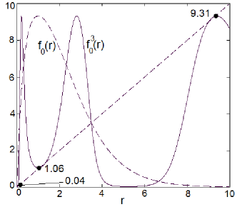
Figure 2: Occurrence of period 3 for the associated interval map

3.4 Further results: convergence to two-cycles

The preceding results indicate that the solutions of (48) and (49) determine the solutions of (43). From Theorem 16 it is evident that complex behavior tends to occur when $d$ is sufficiently large. Otherwise, the solutions of (43) tend to behave more simply as noted in Theorem 10. We now consider the occurrence of two-cycles for a range of values of $d$ that are not too large but extend the range in Theorem 10(b), by examining the following first-order difference equation that is derived from (48) and (49)

$$r_{n+1}=r_{n}e^{d-r_{n}-\gamma r_{n}e^{-r_{n}}},\quad\gamma>0$$ (52)

Lemma 18

If $0<d\leq 2$ then (52) has a unique positive fixed point $\bar{x}$.

Proof. Existence: Let $\eta(x)=d-x-\gamma xe^{-x}$. The nonzero fixed points of (52) must satisfy $e^{\eta(x)}=1$, i.e. $\eta(x)=0$. Since $\eta(0)=d>0$ and $\eta(d)=-\gamma de^{-d}<0$ there is a real number $\bar{x}\in(0,a)$ such that $\eta(\bar{x})=0$. This proves existence.

Uniqueness: Note that $\eta^{\prime}(x)=-1-\gamma e^{-x}+\gamma xe^{-x}$.

Case 1: $\gamma\leq e$; The function $xe^{-x}$ is maximized on $(0,\infty)$ at $h(1)=e^{-1}$ so

$$\eta^{\prime}(x)=-1-\gamma e^{-x}+\gamma xe^{-x}\leq-1+1-\gamma e^{-x}=-\gamma e^{-x}<0$$

It follows that $\eta(x)$ is decreasing on $(0,\infty)$ for this case and has a unique zero that occurs at $\bar{x}$.

Case 2: $e<\gamma<e^{2}$; Consider the function $p(x)=x+\gamma xe^{-x}$. Now

$$p^{\prime}(x)=1+\gamma e^{-x}-\gamma xe^{-x}=e^{-x}(e^{x}+\gamma-\gamma x)$$

The function $q(x)=e^{x}+\gamma-\gamma x$ attains a minimum value at $x=\ln(\gamma)$ since $q^{\prime}(x)=e^{x}-\gamma$. Furthermore,

$$q(\ln(\gamma))=2\gamma-\gamma\ln(\gamma)=\gamma(2-\ln(\gamma))>0$$

for $\gamma<e^{2}$. This implies that $p^{\prime}(x)>0$ on $(0,\infty)$ and therefore $p(x)$ is increasing on $(0,\infty)$. Since $\eta(x)=d-p(x)$, this implies that $\eta(x)$ is decreasing on $(0,\infty)$ and therefore it has a unique zero that occurs at $\bar{x}$.

Case 3: $\gamma>e^{2}$; In this case, we know that $\eta(x)$ is decreasing on $[0,1]$ and $\eta(x)<0$ for $x\in[d,\infty)$. Thus it remains to establish that $\eta(x)<0$ on $(1,d)$.

$$\eta(x)=d-x-\gamma xe^{-x}<d-1-e^{2-x}<d-2\leq 0$$

Thus $\eta(x)$ has a unique zero that occurs at $\bar{x}$ and this completes the proof for all the above cases.   

The above observations also indicate that $\eta(x)>0$ for $x\in(0,\bar{x})$ and $\eta(x)<0$ for $x\in(\bar{x},\infty)$, which we will use in our further analysis. Before examining the stability profile of $\bar{x}$, we need to explore the properties of the function $f(x)$.

Since $f(x)=xe^{d-x-\gamma xe^{-x}}=xe^{\eta(x)}$, then $f^{\prime}(x)=e^{\eta(x)}+x\eta^{\prime}(x)e^{\eta(x)}$. By direct calculations, $f^{\prime}(x)$ can be written as

$$f^{\prime}(x)=e^{\eta(x)}(1-x)(1-\gamma xe^{-x})$$

It follows that $f$ has critical points when $x=1$ and $1-\gamma xe^{-x}=0$. Now we consider the function $\phi(x)=1-\gamma xe^{-x}$, which has a critical point at $x=1$, since $\phi^{\prime}(x)=\gamma e^{-x}(1-x)$. Hence it is decreasing on $(0,1)$ and increasing on $(1,\infty)$ and $\phi(1)=1-\frac{\gamma}{e}$ is the minimum of the function.

(i) When $\gamma<e$, then $\phi(1)>0$, so $\phi(x)>0$ on $(0,\infty)$, hence $f(x)$ has only one critical point at $x=1$. When $\gamma=e,\phi(1)=0$, and again, the only critical point of $f(x)$ occurs at $x=1$. We further break down the case of $\gamma\leq e$ into the following subcases:

a. When $d<1+\frac{\gamma}{e}$, $\eta(1)=d-1-\frac{\gamma}{e}<0$, thus $\bar{x}<1$. Moreover, $f(1)=d-1-\frac{\gamma}{e}<1$, which lets us conclude that $f(x)<1$ for all $x\in(0,\infty)$.

b. When $d\geq 1+\frac{\gamma}{e}$, $\eta(1)=d-1-\frac{\gamma}{e}\geq 0$. This implies that $\bar{x}>1$ if $d>1+\frac{\gamma}{e}$ and $\bar{x}=1$ if $d=1+\frac{\gamma}{e}$.

(ii) When $\gamma>e,\phi(1)<0$, so $f(x)$ has three critical points at $x^{\prime}<1,x^{\prime}=1,x^{\prime\prime}>1$.

On $(0,x^{\prime})$, $1-x>0$ and $\phi(x)>0$, so $f$ is increasing. On $(x^{\prime},1)$, $1-x>0$ and $\phi(x)<0$, so $f$ is decreasing. On $(1,x^{\prime\prime})$, $1-x<0$ and $\phi(x)<0$, so $f$ is increasing. On $(x^{\prime\prime},\infty)$, $1-x<0$ and $\phi(x)>0$, so $f$ is decreasing. By the above observations, it follows that $x^{\prime},x^{\prime\prime}$ are local maxima and $1$ is a minimum point. Next observe that

$$f(1)=e^{2-1-\frac{\gamma}{e}}<1$$

Given that $\gamma x^{\prime}e^{-x^{\prime}}=\gamma x^{\prime\prime}e^{-x^{\prime\prime}}=1$,

$$f(x^{\prime})=x^{\prime}e^{d-x^{\prime}-\gamma x^{\prime}e^{-x^{\prime}}}=x^{\prime}e^{d-x^{\prime}-1}<x^{\prime}e^{2-x^{\prime}-1}=x^{\prime}e^{1-x^{\prime}}$$

Similarly, $f(x^{\prime\prime})<x^{\prime\prime}e^{1-x^{\prime\prime}}$. Now, the function $s(x)=xe^{1-x}$ attains its maximum at $x=1$, since $s^{\prime}(x)=(1-x)e^{1-x}$. Since $s(1)=1$, this implies that $s(x)<1$ for all $x\neq 1,x>0$. This implies that $f(x^{\prime}),f(x^{\prime\prime})<1$ as well, thus for this case $f(x)<1$ for all $x\in(0,\infty).$

Now we establish the global stability of $\bar{x}$.

Lemma 19

If $0<d\leq 2$ then every solution to (52) from positive initial values converges to $\bar{x}$.

Proof. We establish convergence to $\bar{x}$ by showing that $|f(x)-\bar{x}|<|x-\bar{x}|$ for $x\neq\bar{x}$. This is equivalent to

$$x <f(x)<2\bar{x}-x\;\;\text{for}\;\;x<\bar{x}$$ (53a)

$$x >f(x)>2\bar{x}-x\;\;\text{for}\;\;x>\bar{x}$$ (53b)

The first inequalities in (53a-53b) are straightforward to establish: since $\eta(x)>0$ for $x<\bar{x}$ and $\eta(x)<0$ for $x>\bar{x}$, then $f(x)=xe^{\eta(x)}>x$ if $x<\bar{x}$ and $f(x)=xe^{\eta(x)}<x$ if $x>\bar{x}$.

To establish the second inequalities in (53a)-(53b), let

$$t(x)=f(x)+x-2\bar{x}$$

Notice that $t(0)=-2\bar{x}<0$ and $t(\bar{x})=0$. We now show that the inequalities $f(x)<2\bar{x}-x$ for $x<\bar{x}$ and $f(x)>2\bar{x}-x$ for $x>\bar{x}$ are equivalent to $t(x)<0$ for $x<\bar{x}$ and $t(x)>0$ for $x>\bar{x}$, respectively. We establish this by showing that $t(x)$ is strictly increasing on $(0,\infty)$, i.e.

$$t^{\prime}(x)=f^{\prime}(x)+1>0\;\;\text{for}\;\;x>0$$

We establish the above result by considering two cases: Case 1: $\gamma\leq e$; recall that $f(x)$ is maximized at the unique critical point $x=1$. Thus $f^{\prime}(x)>0$ for $x<1$ and $f^{\prime}(x)<0$ for $x>1$. We also showed that $1-\gamma xe^{-x}>0$ for $x>0$. Thus for all $x>1$, since $d\leq 2$

$$|f^{\prime}(x)| \leq e^{2-x-\gamma xe^{-x}}(x-1)(1-\gamma xe^{-x})$$

$$=(x-1)e^{1-x}e^{1-\gamma xe^{-x}}(1-\gamma xe^{-x})$$

$$<e^{-1}e^{1-\gamma xe^{-x}}(1-\gamma xe^{-x})$$

$$=e^{-\gamma xe^{-x}}(1-\gamma xe^{-x})<1$$

i.e. $t^{\prime}(x)>0$ for $x>0$ and inequalities in (53a)-(53b) follow.

Case 2: $\gamma>e$; in this case, $f(x)$ has three critical points occurring at $x^{\prime}<1$, $1$ and $x^{\prime\prime}>1$, where $x^{\prime}$ and $x^{\prime\prime}$ are maxima and $1$ is a minimum. Thus

$$f^{\prime}(x) >0\;\;\text{and}\;\;1-\gamma xe^{-x}>0\;\;\text{for}\;\;x\in(0,x^{\prime})$$

$$f^{\prime}(x) <0\;\;\text{and}\;\;1-\gamma xe^{-x}<0\;\;\text{for}\;\;x\in(x^{\prime},1)$$

$$f^{\prime}(x) >0\;\;\text{and}\;\;1-\gamma xe^{-x}<0\;\;\text{for}\;\;x\in(1,x^{\prime\prime})$$

$$f^{\prime}(x) <0\;\;\text{and}\;\;1-\gamma xe^{-x}>0\;\;\text{for}\;\;x\in(x^{\prime\prime},\infty)$$

Thus $f^{\prime}(x)<0$ if either $x<1$ and $1-\gamma xe^{-x}<0$ or $x>1$ and $1-\gamma xe^{-x}>0$. If $x<1$ and $1-\gamma xe^{-x}<0$, then

$$|f^{\prime}(x)| \leq e^{2-x-\gamma xe^{-x}}(1-x)(\gamma xe^{-x}-1)$$

$$=(\gamma xe^{-x}-1)e^{1-\gamma xe^{-x}}e^{1-x}(1-x)$$

$$<e^{-1}e^{1-x}(1-x)$$

$$=e^{-x}(1-x)<1$$

If $x>1$ and $1-\gamma xe^{-x}>0$, then

$$|f^{\prime}(x)| \leq e^{2-x-\gamma xe^{-x}}(x-1)(1-\gamma xe^{-x})$$

$$=(x-1)e^{1-x}(1-\gamma xe^{-x})e^{1-\gamma xe^{-x}}$$

$$<e^{-1}e^{1-\gamma xe^{-x}}(1-\gamma xe^{-x})$$

$$=e^{-\gamma xe^{-x}}(1-\gamma xe^{-x})<1$$

In either case, if $f(x)$ is decreasing then $-1<f^{\prime}(x)<0$, thus $t^{\prime}(x)=f^{\prime}(x)+1>0$, thus $t(x)$ is increasing for $x>0$, from which the second inequalities in (53a)-(53b) follow.   

By Lemmas 11 and 19, the even and odd terms of (43) converge to $M=\bar{x}_{t_{0}}>0$ and $m=\bar{x}_{t_{1}}>0$, proving the existence and stability of a two-cycle in the sense described in Theorem 16(c). Since $M$ and $m$ must satisfy

$$m=Me^{d-M-m}\;\;\text{and}\;\;M=me^{d-m-M}$$

and

$$Mm=mMe^{2d-2(M+m)}\;\;\text{i.e.}\;\;\;e^{2d-2(M+m)}=1$$

we conclude that $M+m=d$. Thus the following extension of Theorem 10(b) is obtained.

Theorem 20

Let $0<d\leq 2.$ Then every non-constant, positive solution of (43) converges, in the sense of Theorem 16(c), to a two-cycle $\{\rho_{1},\rho_{2}\}$ that satisfy $\rho_{1}+\rho_{2}=d,$ i.e. the mean value of the limit cycle is the fixed point $\bar{r}=d/2.$

As previously mentioned, (43) is valid when $c_{1,n}>0$ has period 2. In this case, the solution of (34) corresponding to $\{r_{n}\}$ of (43) is $x_{n}=r_{n}/c_{1,n}$ which also converges to a sequence of period 2. Thus we have the following corollary.

Corollary 21

Assume in the system (31)-(32) that $\sigma_{1,n}=\sigma_{1}$, $\alpha_{n}=\alpha$, $\beta_{n}=\beta$ are positive constants and $c_{2,n}=\sigma_{1}c_{1,n}$ for all $n$ where $c_{1,n}$ has period two with $c_{1,2k-1}=\xi_{1}$ and $c_{1,2k}=\xi_{2}$ where $\xi_{1},\xi_{2}>0$.

(a) If $\alpha+\ln(\sigma_{1}\beta)\in(0,2]$ then every orbit $\{(x_{n},y_{n})\}$ is determined as

$$x_{n}=\frac{r_{n}}{c_{1,n}},\quad y_{n}=\frac{r_{n+1}}{\sigma_{1}c_{1,n+1}}.$$

(b) Every orbit in the positive quadrant converges to a two-cycle

$$\left\{\left(\frac{\rho_{1}}{\xi_{1}},\frac{\rho_{2}}{\sigma_{1}\xi_{2}}\right),\left(\frac{\rho_{2}}{\xi_{2}},\frac{\rho_{1}}{\sigma_{1}\xi_{1}}\right)\right\}$$

where $\rho_{i}=\lim_{k\rightarrow\infty}r_{2k-i}$ for $i=1,2$ and $\rho_{1}+\rho_{2}=\alpha+\ln(\sigma_{1}\beta).$

3.5 A concluding remark on multistability

We finally mention a feature of (43) that may make its multistable nature less surprising. Consider the following class of nonautonomous first-order equations

$$x_{n+1}=x_{n}e^{\gamma_{n}-\theta_{n}x_{n}}$$

where $\gamma_{n},\theta_{n}$ are given sequences of period 2 with $\theta_{n}>0$ for all $n$. The change of variable $u_{n}=\theta_{n}x_{n}$ reduces this equation to

$$u_{n+1}=u_{n}e^{c_{n}-u_{n}},\quad c_{n}=\gamma_{n}+\ln\frac{\theta_{n+1}}{\theta_{n}}$$ (54)

This equation can be written as

$$u_{n+1}=u_{n-1}e^{c_{n-1}-u_{n-1}}=u_{n-1}e^{c_{n-1}+c_{n}-u_{n-1}-u_{n}}$$

Since $c_{n}$ has period 2, the sum $c_{n-1}+c_{n}=d$ is a constant and (43) is obtained.

If $r_{-1}=u_{0}$ and $r_{0}=u_{1}=u_{0}e^{c_{0}-u_{0}}$ then the corresponding solution of (43) is the solution of (54) with the arbitrary initial value $u_{0}.$ Therefore, all solutions of (54) appear among the solutions of (43) but not conversely. In fact, if $c_{n}^{\prime}$ is any other sequence of period 2 such that $c_{n}^{\prime}+c_{n-1}^{\prime}=d$ then while

$$u_{n+1}=u_{n}e^{c_{n}^{\prime}-u_{n}}$$

is a different equation than (54), it yields exactly the same second-order equation (43). Hence, the following assertion is justified:

Proposition 22

The solutions of (43) include the solutions of all first-order equations of type (54) with $c_{n}+c_{n-1}=d.$

The coexistence of solutions of so many different first-order equations among the solutions of (43) is a further indication of the diversity of solutions that the latter may exhibit.

4 Conclusion and future directions

In this paper we examine the dynamics of the non-autonomous system (1)-(2) whose special cases appear in stage-structured models of populations that are of Ricker type, or overcompensatory. In Section 2 we obtain conditions that imply uniform boundedness as well as global convergence to zero with variable parameters. In biological models these results give general conditions for the species’ extinction. We have also shown that in periodic environments certain stocking strategies do not prevent extinction.

In Section 3 we study the dynamics of a special case of the system that is mathematically interesting. We use semiconjugate factorization to show that in a wider range of parameters than what is considered in [3] complex and multistable behavior occurs.

The results in Section 3 concern Equation (43) which is autonomous (even if the system is not). For future investigation one may consider the more general, non-autonomous equation (38) with periodic $d_{n}.$ Preliminary work on this periodic case shows that the dynamics of (38) where $d_{n}$ has an odd period (including the autonomous case $p=1$) is substantially and qualitatively different from the case where $d_{n}$ has an even period.

Another generalization of (43), namely the autonomous equation

$$r_{n+1}=r_{n-1}e^{d-br_{n-1}-cr_{n}}$$ (55)

where $b,c>0$ exhibits different dynamics than (43) when $b\not=c.$ In particular, we expect that mulitstable orbits will not occur although complex behavior is possible. There is currently no comprehensive study of the dynamics of (55) that we are aware of so obtaining significant details on the dynamics of this equation would be desirable.

References

• [1] Ackleh, A.S. and Jang, S.R.-J., A discrete two-stage population model: continuous versus seasonal reproduction, J. Difference Eq. Appl. 13, 261-274, 2007
• [2] Cushing, J.M., A juvenile-adult model with periodic vital rates, J. Math Biology, 53, pp.520-539, 2006
• [3] Franke, J.E., Hoag, J.T. and Ladas, G., Global attractivity and convergence to a two-cycle in a difference equation, J. Difference Eq. Appl. 5, 203-209, 1999
• [4] Giordano, G. and Lutscher, F., Harvesting and predation of a sex- and age-structured population, J. Biol. Dyn. 5, 600-618, 2011
• [5] Li, T-Y and Yorke, J.A., Period three implies chaos, Amer. Math. Monthly 82, 985-992, 1975
• [6] Liz, E. and Pilarczyk, P., Global dynamics in a stage-sturctured discrete-time population model with harvesting, J. Theor. Biol. 297, 148-165, 2012
• [7] Sedaghat, H., Form Symmetries and Reduction of Order in Difference Equations, CRC Press, Boca Raton, 2011
• [8] Sedaghat, H., Global attractivity in a class of non-autonomous, nonlinear, higher-order difference equations, J. Difference Eq. and Appl., 19, 1049-1064, 2013
• [9] Sedaghat, H., Semiconjugate factorizations of higher order linear difference equations in rings, J. Difference Eq. and Appl., 20, 251-270, 2014
• [10] Sedaghat, H., Folding, cycles and chaos in planar systems, J. Difference Eq. and Appl., 21, 1-15, 2015
• [11] Zipkin, E.F., Kraft, C.E., Cooch, E.G., and Sullivan, P.J., When can efforts to control nuisance and invasive species backfire? Ecol. Appl. 19, 1585-1595, 2009