The binned bispectrum estimator: template-based and non-parametric CMB non-Gaussianity searches

Abstract

We describe the details of the binned bispectrum estimator as used for the official 2013 and 2015 analyses of the temperature and polarization CMB maps from the ESA Planck satellite. The defining aspect of this estimator is the determination of a map bispectrum (3-point correlation function) that has been binned in harmonic space. For a parametric determination of the non-Gaussianity in the map (the so-called $f_{\mathrm{NL}}$ parameters), one takes the inner product of this binned bispectrum with theoretically motivated templates. However, as a complementary approach one can also smooth the binned bispectrum using a variable smoothing scale in order to suppress noise and make coherent features stand out above the noise. This allows one to look in a model-independent way for any statistically significant bispectral signal. This approach is useful for characterizing the bispectral shape of the galactic foreground emission, for which a theoretical prediction of the bispectral anisotropy is lacking, and for detecting a serendipitous primordial signal, for which a theoretical template has not yet been put forth. Both the template-based and the non-parametric approaches are described in this paper.

1 Introduction

A fundamental question of observational cosmology is whether the primordial cosmological perturbations were precisely Gaussian, or whether small departures from exact Gaussianity can be detected at a statistically significant level and then characterized. Here the qualification ‘primordial’ is essential because our goal is to probe the new physics at play in the very early Universe. However, it is also important to study the non-Gaussianity that was subsequently imprinted at late times through known processes, in particular the nonlinear dynamics of gravitational clustering, in order to ‘decontaminate’ the primordial non-Gaussianity. Observations of the cosmic microwave background (CMB) anisotropies in temperature and polarization are particularly well-suited to addressing this fundamental question, as they provide a clean probe of the initial conditions because most (but not all) of the CMB anisotropy was imprinted well before nonlinear effects became important.

Non-Gaussianity is a vast subject because Gaussian stochastic processes are the exception rather than the rule, comprising a set of measure zero within the space of all possible stochastic processes for generating an initial state. Given the highly exceptional nature of the stochastic processes that are exactly Gaussian, there is a great need to identify departures from Gaussianity that are in some sense theoretically well-motivated. Bispectral non-Gaussianity may be regarded as the leading-order correction to exact Gaussianity in some sort of a perturbative expansion.

Early investigations of the statistics of large-scale structure of the universe, mainly on grounds of simplicity, assumed Gaussian statistics before there was a well-motivated theoretical explanation for why the primordial cosmological perturbations should be very nearly Gaussian. However in the mid-1980s the calculation of the cosmological perturbations generated from quantum vacuum fluctuations during inflation provided a theoretical justification for using Gaussian statistics to model the large-scale structure. Indeed Gaussianity was proclaimed as being one of the core predictions of inflation.

Inflation however does not predict exact Gaussianity no matter what model of inflation is assumed. It cannot be modeled by a free field theory because at a minimum the gravitational sector is nonlinear. Additional nonlinearity will of course also arise from other sources, such as for example from the nonlinearity of the inflationary potential. The departures from Gaussianity predicted within the framework of single-field inflation were calculated by Maldacena [1] and by Acquaviva et al. [2]. Many other inflation models have been introduced in the literature that can produce non-negligible non-Gaussianity. For example, models where multiple scalar fields play a role during inflation, where isocurvature perturbations are generated, or where inflation starts in an excited vacuum state. In some string-based models, as well as in some modified gravity or effective-field theories, the kinetic part of the inflaton Lagrangian can be non-standard, leading to novel bispectral signatures. Deviations from the pure slow-roll phase in the inflaton potential can also produce oscillations in the bispectrum. See e.g., [3] or [4, 5] for a review.

Under the assumption of statistical isotropy, the bispectrum of the map of a scalar quantity reduces to a function of three multipole numbers $B_{\ell_{1}\ell_{2}\ell_{3}}$, where the bispectrum is symmetric under permutations and vanishes unless the $\ell$-triplet satisfies the triangle inequality [6]. If we include polarization, which in turn can be decomposed into $E$ and $B$ components, then the bispectrum needs to be generalized to $B^{p_{1}p_{2}p_{3}}_{\ell_{1}\ell_{2}\ell_{3}}$, where $p_{1},p_{2},p_{3}=T,E$ (we will not consider $B$-polarization in this paper). If we insist on exploiting the highest possible spectral resolution of the CMB maps (not necessarily the best idea), then the number of reduced bispectral coefficients that can be measured is huge, scaling with $\ell_{\mathrm{max}}$ as $\ell_{\mathrm{max}}^{3}$, and the individual coefficients are too contaminated by noise to be useful in detecting bispectral Gaussianity. A major and unavoidable contribution to this noise arises from cosmic variance — that is, from the departures from zero of $B^{p_{1}p_{2}p_{3}}_{\ell_{1}\ell_{2}\ell_{3}}$ that would occur even if the underlying stochastic process were exactly Gaussian. While Gaussianity requires that the expectation value of the bispectral coefficients, calculable only in the limit of an infinite number of sky realizations, vanishes, the value calculated for any single sky realization will include fluctuations about this expectation value. For this reason, in order to make any meaningful detection of bispectral non-Gaussianity in the data, it is necessary to combine, in one way or another, many measured bispectral coefficients in order to make the signal stand out over the noise.

There are basically two situations to be considered. If we have a simple parametric model for the expected pattern of bispectral non-Gaussianity (generally parameterized by an amplitude called $f_{\mathrm{NL}}$), then an optimal estimator can be constructed by summing the observed bispectral coefficients over $\ell_{1},\ell_{2},\ell_{3}$ using inverse variance weighting. Another situation to be considered involves non-parametric reconstruction of the bispectrum, where we do not have a specific template in mind, but want to smooth the bispectrum in order to reduce the noise and see whether there is a broad signal that stands out over the noise at a statistically significant level. This latter approach is particularly relevant for studying the bispectral properties of foregrounds, for which a theory of the expected shape of the bispectral non-Gaussianity is lacking.

Combining the bispectral coefficients is not only required from the physical point of view (to obtain statistically significant results), but also computationally: computing $\mathcal{O}(\ell_{\mathrm{max}}^{3})$ bispectral coefficients for each map is not feasible in practice. A natural solution, motivated by the second case mentioned above as well as the observation that many of the templates of the first case are very smooth, is to bin the bispectrum in harmonic space. This is the basis of the binned bispectrum estimator, which was first described in [7], and which is the subject of this paper (see also [8] for an independent investigation of the binned bispectrum estimator, and [9] for a first rudimentary flat-sky estimator based on a binned bispectrum applied to the MAXIMA data). The binned bispectrum estimator has established itself as one of the three main bispectrum estimators used successfully for the official analysis of the Planck data, both in 2013 [4] and in 2015 [5]. The other two are the KSW estimator [10, 11, 12] and the modal estimator [13, 14, 15], and we will now briefly describe the main methodological differences between these three estimators. In addition, other bispectrum estimators exist, based on wavelets (e.g. [16]), needlets (e.g. [17]), and Minkowski functionals (e.g. [18]) (see [4] for more complete references).

The KSW estimator (separable template fitting) is based on the observation that if the primordial bispectrum template is separable as a function of $k_{1},k_{2},k_{3}$ (or alternatively the CMB bispectrum template is separable as a function of $\ell_{1},\ell_{2},\ell_{3}$ modulo a possible overall integral over $r$, the radial distance towards the surface of last scattering), then the terms in the optimal estimator for $f_{\mathrm{NL}}$ can be reordered as a product of terms depending only on $k_{1},\ell_{1}$, terms depending only on $k_{2},\ell_{2}$, and terms depending only on $k_{3},\ell_{3}$ (within an overall integral over $r$). This significantly reduces the computational cost (by effectively replacing a three-dimensional integral and sum by the product of three one-dimensional integrals and sums), at the cost of losing the ability for full bispectrum reconstruction. The KSW estimator is fast, but only works for separable templates and can only be used for the first case mentioned above (template fitting).

The modal estimator builds on the idea of the KSW estimator by first expanding the theoretical bispectrum templates and the bispectrum of the map in a basis of separable templates, the so-called modes. (For the Planck 2015 analysis two pipelines were used, one with a basis of 600 polynomials, and the other with 2000.) The coefficients of the individual modes are then computed using the KSW technique. In this way one can in principle treat any bispectrum template, separable or not, as well as reconstruct the full bispectrum of the map. These advantages come at the cost of often needing a large number of modes for sufficient convergence, which can become computationally heavy.

The binned bispectrum estimator does not use the KSW technique and keeps the full three-dimensional sum. The required computational reduction comes from reducing the number of terms in the sum by binning the bispectrum in harmonic space, as will be discussed in detail in this paper. In this way one can do both template fitting (with templates that do not need to be separable) and full bispectrum reconstruction as mentioned above. Moreover, the estimator is very fast when applied to a map, has a convenient modular structure (which means for example that one can analyze an additional template without having to rerun the map), and gives the dependence of $f_{\mathrm{NL}}$ on $\ell$ as a free bonus. The possible drawback is that the method works only for bispectra that are relatively smooth (or have rapid oscillations only in a limited $\ell$-range) in order for a limited number of bins (about 50–60 in practice) to suffice.

The basic output of the binned bispectrum estimator is a binned, or coarse-grained, pseudo-bispectrum. Here ‘pseudo’ indicates that full-sky spherical harmonic transforms have been applied to a masked sky, so that the recovered $a_{\ell m}$ coefficients are in fact a convolution of the real CMB multipole coefficients with the multipole coefficients of the mask. How one corrects for the artefacts of the mask is discussed in detail in Section 4. Below we shall almost always assume the presence of a mask but will omit the qualification ‘pseudo’. The coarse-grained pseudo-bispectrum can be combined with a library of theoretical templates by means of an inner product that generates optimally matched filters. This approach was described in [7], where it was shown that with a modest number of bins, the loss of information compared to an unbinned analysis is negligible. One can thus determine the so-called $f_{\mathrm{NL}}$ parameter for various templates, but one can also construct other estimators, for example to look for the acoustic peaks in the bispectrum (see [7]).

Section 2 describes the binned bispectrum and how it is calculated from a sky map. Because there have been many refinements of the binned estimator (such as its generalization to include polarization) since the previous paper, we will discuss the parametric analysis in detail in Section 3. As mentioned above, Section 4 describes how to deal with the masked sky. The implementation details of the code are discussed in Section 5. The binned bispectrum can also be used to carry out a non-parametric, or model-independent, analysis. In such an analysis the binned bispectrum can be smoothed to search for a serendipitous statistically significant signal of bispectral non-Gaussianity in the CMB for which templates have not yet been proposed, or to characterize the bispectral properties of foregrounds without a well-motivated theoretical template. The construction of the full smoothed bispectrum is treated in Section 6. The smoothing complicates the statistical analysis of the significance of any non-Gaussian features because it introduces correlations between neighbouring bins. In Section 7 we develop a method to address this complication and provide an illustration by applying it to the bispectrum of a realistic map containing a Gaussian CMB and radio point sources. Some conclusions are presented in Section 8. Appendix A provides both a further discussion of the templates of Section 3 and a further illustration of the techniques of Section 6 by presenting two-dimensional cross-sections of the smoothed template bispectra.

2 Binned bispectrum estimator

2.1 Binned bispectrum

In this paper we define the bispectrum by means of the expectation value

$$B_{\ell_{1}\ell_{2}\ell_{3}}^{p_{1}p_{2}p_{3}}=\left\langle\int d\hat{\Omega}\,M_{\ell_{1}}^{p_{1}}(\hat{\Omega})M_{\ell_{2}}^{p_{2}}(\hat{\Omega})M_{\ell_{3}}^{p_{3}}(\hat{\Omega})\right\rangle$$ (2.1)

where $M_{\ell}^{p}(\hat{\Omega})$ is a map (as a function of position $\hat{\Omega}$ on the celestial sphere) where all but the $(2\ell+1)$ components having multipole number $\ell$ in the spherical harmonic decomposition have been filtered out, so that

$$M_{\ell}^{p}(\hat{\Omega})=\sum_{m=-\ell}^{+\ell}a_{\ell m}^{p}Y_{\ell m}(\hat{\Omega}).$$ (2.2)

The label $p$ refers in general to either temperature ($T$), $E$-polarization ($E$), or $B$-polarization ($B$), although in this paper we will only consider the former two. Inserting the expansion (2.2) into (2.1) and using the Gaunt integral $\int d\hat{\Omega}\,Y_{\ell_{1}m_{1}}Y_{\ell_{2}m_{2}}Y_{\ell_{3}m_{3}}=\sqrt{N_{\triangle}}\left(\begin{smallmatrix}\ell_{1}&\ell_{2}&\ell_{3}\cr m_{1}&m_{2}&m_{3}\cr\end{smallmatrix}\right)$, we find that

$$B_{\ell_{1}\ell_{2}\ell_{3}}^{p_{1}p_{2}p_{3}}=\sqrt{N_{\triangle}^{\ell_{1}\ell_{2}\ell_{3}}}\sum_{m_{1},m_{2},m_{3}}\begin{pmatrix}\ell_{1}&\ell_{2}&\ell_{3}\cr m_{1}&m_{2}&m_{3}\cr\end{pmatrix}\langle a_{\ell_{1}m_{1}}^{p_{1}}a_{\ell_{2}m_{2}}^{p_{2}}a_{\ell_{3}m_{3}}^{p_{3}}\rangle,$$ (2.3)

where we have defined

$$N_{\triangle}^{\ell_{1}\ell_{2}\ell_{3}}\equiv\frac{(2\ell_{1}+1)(2\ell_{2}+1)(2\ell_{3}+1)}{4\pi}\begin{pmatrix}\ell_{1}&\ell_{2}&\ell_{3}\cr 0&0&0\cr\end{pmatrix}^{2},$$ (2.4)

which may be interpreted as the number of possible $(\ell_{1},\ell_{2},\ell_{3})$ triangles on the celestial sphere. (This quantity is sometimes denoted as $h_{\ell_{1}\ell_{2}\ell_{3}}^{2}$ in the literature.) The quantity $\langle a_{\ell_{1}m_{1}}^{p_{1}}a_{\ell_{2}m_{2}}^{p_{2}}a_{\ell_{3}m_{3}}^{p_{3}}\rangle$ is the CMB angular bispectrum, while the quantity $B_{\ell_{1}\ell_{2}\ell_{3}}^{p_{1}p_{2}p_{3}}/N_{\triangle}^{\ell_{1}\ell_{2}\ell_{3}}$ is known as the reduced bispectrum.

From these equations we can derive two mathematical properties of the bispectrum. Firstly, the bispectrum is symmetric under the simultaneous interchange of its three multipole numbers $\ell_{1},\ell_{2},\ell_{3}$ and its three polarization indices $p_{1},p_{2},p_{3}.$ This means that it is sufficient to consider only the subspace $\ell_{1}\leq\ell_{2}\leq\ell_{3}$. It should be noted, however, that once we have both temperature and polarization, imposing this condition means that we no longer have the freedom to rearrange the polarization indices, so that for example the $TTE$, $TET$, and $ETT$ combinations correspond to three distinct bispectra. Secondly, because of the presence of the Wigner $3j$-symbol with all $m$’s equal to zero in (2.4), both the parity condition ($\ell_{1}+\ell_{2}+\ell_{3}$ even) and the triangle inequality (consisting of $|\ell_{1}-\ell_{2}|\leq\ell_{3}\leq\ell_{1}+\ell_{2}$ and permutations thereof) must be satisfied. Otherwise the bispectrum coefficient vanishes. Note that the parity condition is a consequence of our starting point (2.1). One could also define the angle-averaged bispectrum as in (2.3) but without the $\sqrt{N_{\triangle}}$ factor in front. That expression would still include parity-odd modes as well in principle. The parity condition is a selection rule that results under the assumption that the underlying stochastic process is invariant under spatial inversion, which is the case for example for most scalar field models of inflation. In that case the odd-parity bispectrum can only be noise from cosmic variance and thus is not worth analyzing. In this paper we do not consider parity-odd combinations involving $B$-polarization or chiral models where parity is not a good symmetry (like in the standard electroweak model). See for example [20, 21, 22] for studies of parity-odd bispectra.

To compute the observed bispectrum with the maximum possible resolution, we would simply evaluate the integral over the sky of triple products of maximally filtered observed sky maps

$$B_{\ell_{1}\ell_{2}\ell_{3}}^{p_{1}p_{2}p_{3},\mathrm{obs}}=\int d\hat{\Omega}\,M_{\ell_{1}}^{p_{1},\mathrm{obs}}(\hat{\Omega})M_{\ell_{2}}^{p_{2},\mathrm{obs}}(\hat{\Omega})M_{\ell_{3}}^{p_{3},\mathrm{obs}}(\hat{\Omega})$$ (2.5)

for each distinct triplet satisfying the above selection rules. (In practice this integral is evaluated as a sum over pixels.) The total number of triplets would be $\mathcal{O}(10^{7})$ for a WMAP or $\mathcal{O}(10^{9})$ for a Planck temperature map.

But we can also use broader filters for the integral in (2.5), as we shall see later with very little loss of information because a modest resolution in $\ell$ suffices for many physically motivated templates for which the predicted $B_{\ell_{1}\ell_{2}\ell_{3}}^{p_{1}p_{2}p_{3}}$ varies slowly with its $\ell$ arguments. We end up having to compute only $\mathcal{O}(10^{4})$ bin triplets, leading to an enormous reduction in the computational resources required. We divide the $\ell$-range $[\ell_{\mathrm{min}},\ell_{\mathrm{max}}]$ into subintervals denoted by $\Delta_{i}=[\ell_{i},\ell_{i+1}-1]$ where $i=0,\ldots,(N_{\mathrm{bins}}-1)$ and $\ell_{N_{\mathrm{bins}}}=\ell_{\mathrm{max}}+1$, so that the filtered maps are

$$M_{i}^{p}(\Omega)=\sum_{\ell\in\Delta_{i}}\sum_{m=-\ell}^{+\ell}a_{\ell m}^{p}Y_{\ell m}(\hat{\Omega}),$$ (2.6)

and we use these instead of $M_{\ell}^{p}$ in the expression for the bispectrum (2.5). The binned bispectrum is

$$B_{i_{1}i_{2}i_{3}}^{p_{1}p_{2}p_{3},\mathrm{obs}}=\frac{1}{\Xi_{i_{1}i_{2}i_{3}}}\int d\hat{\Omega}\,M_{i_{1}}^{p_{1},\mathrm{obs}}(\hat{\Omega})M_{i_{2}}^{p_{2},\mathrm{obs}}(\hat{\Omega})M_{i_{3}}^{p_{3},\mathrm{obs}}(\hat{\Omega})$$ (2.7)

where $\Xi_{i_{1}i_{2}i_{3}}$ is the number of $\ell$ triplets within the $({i_{1},i_{2},i_{3}})$ bin triplet satisfying the triangle inequality and parity condition selection rule. Because of this normalization factor, $B_{i_{1}i_{2}i_{3}}^{p_{1}p_{2}p_{3}}$ may be considered an average over all valid $B_{\ell_{1}\ell_{2}\ell_{3}}^{p_{1}p_{2}p_{3}}$ inside the bin triplet.

2.2 Variance

We start by considering only the temperature bispectrum. The covariance of the bispectra $B_{\ell_{1}\ell_{2}\ell_{3}}$ and $B_{\ell_{4}\ell_{5}\ell_{6}}$ equals the average of the product minus the product of the averages. Under the assumption of weak non-Gaussianity the calculation simplifies significantly. In that case one can neglect the average value of the bispectra, and the average of the product,

$$\langle B_{\ell_{1}\ell_{2}\ell_{3}}B_{\ell_{4}\ell_{5}\ell_{6}}\rangle= \sqrt{N_{\triangle}^{\ell_{1}\ell_{2}\ell_{3}}N_{\triangle}^{\ell_{4}\ell_{5}\ell_{6}}}$$

$$\times\sum_{\tiny\begin{array}[]{c@{}c@{}c}m_{1},&m_{2},&m_{3},\\ m_{4},&m_{5},&m_{6}\\ \end{array}}\!\!\!\!\begin{pmatrix}\ell_{1}&\ell_{2}&\ell_{3}\cr m_{1}&m_{2}&m_{3}\cr\end{pmatrix}\begin{pmatrix}\ell_{4}&\ell_{5}&\ell_{6}\cr m_{4}&m_{5}&m_{6}\cr\end{pmatrix}\langle a_{\ell_{1}m_{1}}a_{\ell_{2}m_{2}}a_{\ell_{3}m_{3}}a_{\ell_{4}m_{4}}^{*}a_{\ell_{5}m_{5}}^{*}a_{\ell_{6}m_{6}}^{*}\rangle$$ (2.10)

(using the fact that $B$ is real so that $B=B^{*}$), can be rewritten as the product of three power spectra $C_{\ell}\equiv\langle a_{\ell m}a_{\ell m}^{*}\rangle$ using Wick’s theorem

$$\langle a_{\ell_{1}m_{1}} a_{\ell_{2}m_{2}}a_{\ell_{3}m_{3}}a_{\ell_{4}m_{4}}^{*}a_{\ell_{5}m_{5}}^{*}a_{\ell_{6}m_{6}}^{*}\rangle=C_{\ell_{1}}C_{\ell_{2}}C_{\ell_{3}}[\delta_{\ell_{1}\ell_{4}}\delta_{\ell_{2}\ell_{5}}\delta_{\ell_{3}\ell_{6}}\delta_{m_{1}m_{4}}\delta_{m_{2}m_{5}}\delta_{m_{3}m_{6}}$$

$$+(14)(26)(35)+(15)(24)(36)+(15)(26)(34)+(16)(24)(35)+(16)(25)(34)],$$ (2.11)

using obvious shorthand to denote the other permutations of $\delta$-functions. Due to the $\delta$-functions, the covariance matrix is diagonal, so we need to consider only the (diagonal) variance of $B_{\ell_{1}\ell_{2}\ell_{3}}$. We use the identity

$$\sum_{m_{1}m_{2}m_{3}}\begin{pmatrix}\ell_{1}&\ell_{2}&\ell_{3}\cr m_{1}&m_{2}&m_{3}\cr\end{pmatrix}\begin{pmatrix}\ell_{1}&\ell_{2}&\ell_{3}\cr m_{1}&m_{2}&m_{3}\cr\end{pmatrix}=1$$ (2.12)

and the fact that for even parity of $\ell_{1}+\ell_{2}+\ell_{3}$ the columns of the Wigner $3j$-symbol can be permuted to obtain

$${\rm Var}(B_{\ell_{1}\ell_{2}\ell_{3}})=g_{\ell_{1}\ell_{2}\ell_{3}}N_{\triangle}^{\ell_{1}\ell_{2}\ell_{3}}C_{\ell_{1}}C_{\ell_{2}}C_{\ell_{3}}\equiv V_{\ell_{1}\ell_{2}\ell_{3}}$$ (2.13)

with $g_{\ell_{1}\ell_{2}\ell_{3}}$ equal to 6, 2, or 1, depending on whether 3, 2, or no $\ell$’s are equal, respectively, and $N_{\triangle}$ defined as in (2.4). Similarly the variance of the binned bispectrum $B_{i_{1}i_{2}i_{3}}=({\Xi_{i_{1}i_{2}i_{3}}})^{-1}\sum_{\ell_{1}\in\Delta_{1}}\sum_{\ell_{2}\in\Delta_{2}}\sum_{\ell_{3}\in\Delta_{3}}B_{\ell_{1}\ell_{2}\ell_{3}}$ is given by

$${\rm Var}(B_{i_{1}i_{2}i_{3}})=\frac{g_{i_{1}i_{2}i_{3}}}{(\Xi_{i_{1}i_{2}i_{3}})^{2}}\sum_{\ell_{1}\in\Delta_{1}}\sum_{\ell_{2}\in\Delta_{2}}\sum_{\ell_{3}\in\Delta_{3}}N_{\triangle}^{\ell_{1}\ell_{2}\ell_{3}}C_{\ell_{1}}C_{\ell_{2}}C_{\ell_{3}}\equiv V_{i_{1}i_{2}i_{3}}$$ (2.14)

with $g_{i_{1}i_{2}i_{3}}$ equal to 6, 2, or 1, depending on whether 3, 2, or no $i$’s are equal, respectively. The $\delta$-functions in (2.11) lead here to conditions of equality on the bins, since due to the sum over all $\ell$’s inside a bin, $\delta_{\ell_{a}\ell_{b}}$ will always give 1 if $\ell_{a}$ and $\ell_{b}$ are in the same bin, and 0 if not.

With the noise and beam smoothing present in a real experiment, (2.14) becomes

$$V_{i_{1}i_{2}i_{3}}=\frac{g_{i_{1}i_{2}i_{3}}}{(\Xi_{i_{1}i_{2}i_{3}})^{2}}\sum_{\ell_{1}\in\Delta_{1}}\sum_{\ell_{2}\in\Delta_{2}}\sum_{\ell_{3}\in\Delta_{3}}N_{\triangle}^{\ell_{1}\ell_{2}\ell_{3}}(b_{\ell_{1}}^{2}C_{\ell_{1}}+N_{\ell_{1}})(b_{\ell_{2}}^{2}C_{\ell_{2}}+N_{\ell_{2}})(b_{\ell_{3}}^{2}C_{\ell_{3}}+N_{\ell_{3}})$$ (2.15)

where $b_{\ell}$ is the beam transfer function and $N_{\ell}$ the instrument noise power spectrum. This expression is exact only for an axisymmetric beam and isotropic noise; otherwise it is an approximation (because the beam and noise properties would include off-diagonal matrix elements). For a Gaussian beam, the beam transfer function is typically specified by the full width at half maximum $\theta_{\mathrm{FWHM}}$ (in radians), so that $b_{\ell}=\exp\left[-\frac{1}{2}\ell(\ell+1)\theta^{2}_{\mathrm{FWHM}}/(8\ln 2)\right].$ A pixel window function $w_{\ell}$ to account for pixelization effects is combined with the beam transfer function according to $b_{\ell}\rightarrow w_{\ell}b_{\ell}$.

For bispectral elements including both $T$ and $E$, the variance is replaced by the covariance matrix in polarization space, whose expression without binning is

$$\mathrm{Covar}(B_{\ell_{1}\ell_{2}\ell_{3}}^{p_{1}p_{2}p_{3}},B_{\ell_{1}\ell_{2}\ell_{3}}^{p_{4}p_{5}p_{6}})=g_{\ell_{1}\ell_{2}\ell_{3}}N_{\triangle}^{\ell_{1}\ell_{2}\ell_{3}}(\tilde{C}_{\ell_{1}})^{p_{1}p_{4}}(\tilde{C}_{\ell_{2}})^{p_{2}p_{5}}(\tilde{C}_{\ell_{3}})^{p_{3}p_{6}}\equiv V_{\ell_{1}\ell_{2}\ell_{3}}^{p_{1}p_{2}p_{3}p_{4}p_{5}p_{6}},$$ (2.16)

where

$$\tilde{C}_{\ell}=\left(\begin{array}[]{cc}(b_{\ell}^{T})^{2}C_{\ell}^{TT}+N_{\ell}^{T}&b_{\ell}^{T}b_{\ell}^{E}C_{\ell}^{TE}\\ b_{\ell}^{T}b_{\ell}^{E}C_{\ell}^{TE}&(b_{\ell}^{E})^{2}C_{\ell}^{EE}+N_{\ell}^{E}\end{array}\right).$$ (2.17)

Here noise uncorrelated in $T$ and $E$ has been assumed. Similarly, for the binned case

$$\mathrm{Covar}(B_{i_{1}i_{2}i_{3}}^{p_{1}p_{2}p_{3}},B_{i_{1}i_{2}i_{3}}^{p_{4}p_{5}p_{6}}) =\frac{g_{i_{1}i_{2}i_{3}}}{(\Xi_{i_{1}i_{2}i_{3}})^{2}}\sum_{\ell_{1}\in\Delta_{1}}\sum_{\ell_{2}\in\Delta_{2}}\sum_{\ell_{3}\in\Delta_{3}}N_{\triangle}^{\ell_{1}\ell_{2}\ell_{3}}(\tilde{C}_{\ell_{1}})^{p_{1}p_{4}}(\tilde{C}_{\ell_{2}})^{p_{2}p_{5}}(\tilde{C}_{\ell_{3}})^{p_{3}p_{6}}$$

$$\equiv V_{i_{1}i_{2}i_{3}}^{p_{1}p_{2}p_{3}p_{4}p_{5}p_{6}}.$$ (2.18)

Some subtleties arise in the derivation of equation (2.16). The covariance matrix is in principle an $8\times 8$ matrix, given that there are 8 independent polarized bispectra $TTT$, $TTE$, $TET$, $TEE$, $ETT$, $ETE$, $EET$, and $EEE$. As mentioned before, note that for example $TTE$ and $TET$ are not the same: each polarization index $p_{i}$ is coupled to a multipole index $\ell_{i}$, and cannot be exchanged due to the restriction $\ell_{1}\leq\ell_{2}\leq\ell_{3}$ that we will always impose in order to reduce computation time. A naive calculation of this $8\times 8$ matrix appears to lead to a more complicated expression in the case of equal $\ell$’s that is not proportional to $g_{\ell_{1}\ell_{2}\ell_{3}}$. However, one should treat the cases where two or three $\ell$’s are equal separately. For example, when $\ell_{2}=\ell_{3}$, one can exchange the last two polarization indices and one finds that $TTE=TET$ and $ETE=EET$. Hence in that case there are only 6 independent bispectra, and the covariance matrix is $6\times 6$. Similarly, when all three $\ell$’s are equal, the covariance matrix is $4\times 4$.

However, it turns out that as far as computing $f_{\mathrm{NL}}$ is concerned, when evaluating the sum in (3.27), properly treating the special cases where $\ell$’s are equal by reducing the dimension of the covariance matrix and bispectrum vector, the final result is identical to the following calculation: taking the covariance matrix to be the $8\times 8$ matrix as computed in the case of all $\ell$’s unequal, multiplying it by $g_{\ell_{1}\ell_{2}\ell_{3}}$, and then computing the sum in (3.27) directly without treating the cases of equal $\ell$’s separately. This second computation is much more convenient from a practical point of view. Finally it can be shown that the latter expression of the covariance matrix can be rewritten as the separable product involving only $2\times 2$ matrices in (2.16).

Similarly it can be shown that the variances of the combinations $B^{T2E}\equiv TTE+TET+ETT$ and $B^{TE2}\equiv TEE+ETE+EET$ used for the smoothed bispectrum (see Section 6) are also recovered correctly when using (2.16) or (2.18). Here one should use of course that Var($B^{T2E}$) = Var($TTE$) + Var($TET$) + Var($ETT$) + 2 Covar($TTE,TET$) + 2 Covar($TTE,ETT$) + 2 Covar($TET,ETT$), and similarly for Var($B^{TE2}$). So in the end, while one should remember the caveats regarding (2.16) and (2.18) in the case of equal $\ell$’s or $i$’s, for the practical purposes of this paper they can be used without any problem.

2.3 Linear correction term

The definition of the bispectrum in (2.1) assumes a rotationally invariant CMB sky and that the bispectral expectation values have even parity (as a consequence of the parity invariance of the underlying stochastic process, which we assume here). Because of rotational invariance, the $m$ dependence of the expectation can be factored out, and the sample reduced bispectral coefficients provide a lossless compression of the data concerning the bispectrum. However, in a real experiment as opposed to idealized observations of the primordial sky, two sources of anisotropy arise that break rotational invariance and require corrections to the bispectrum estimation to avoid spurious results.

The first is anisotropic superimposed instrument noise, due to for example an anisotropic scanning pattern of the satellite. The second is anisotropy introduced by a mask needed to remove the brightest parts of our galaxy and the strongest point sources. These two anisotropic ‘contaminants’, unlike for example foreground contaminants, cannot be removed by cleaning and must be accounted for in the analysis. These anisotropic contaminants can mimic a primordial bispectrum signal. For example, due to an anisotropic scanning pattern of the experiment, certain (large-scale) areas of the sky may have less (small-scale) noise than other areas. This correlation between large and small scales produces a contaminant bispectrum that peaks in the squeezed limit (bispectrum configurations with one small $\ell$ and two large ones). As explained in the next Section, that is also where the primordial so-called local shape has its main signal. Since the CMB and the noise are uncorrelated, the effect will average out to zero in the central value of the bispectrum over a large number of maps (no bias), but it will increase the variance. And while an unbiased estimator will find the correct central value when averaged over a large number of maps, a larger variance does mean that there is more chance to find a value far from the true one when applied to a single map.

These contaminants can be mitigated by subtracting from the cubic expression of the observed bispectrum given in (2.5) or (2.7) a linear correction term, as shown in [23, 12], that is,

$$B_{i_{1}i_{2}i_{3}}^{p_{1}p_{2}p_{3},\mathrm{obs}}\rightarrow\Bigl{(}B_{i_{1}i_{2}i_{3}}^{p_{1}p_{2}p_{3},\mathrm{obs}}-B_{i_{1}i_{2}i_{3}}^{p_{1}p_{2}p_{3},\mathrm{lin}}\Bigr{)}.$$ (2.19)

‘Cubic’ and ‘linear’ here mean cubic and linear in the observed map, respectively. The linear correction term is

$$B_{i_{1}i_{2}i_{3}}^{p_{1}p_{2}p_{3},\mathrm{lin}}=\int d\hat{\Omega} \left[M_{i_{1}}^{p_{1},\mathrm{obs}}\left\langle M_{i_{2}}^{p_{2},G}M_{i_{3}}^{p_{3},G}\right\rangle\right.$$

$$\left.+M_{i_{2}}^{p_{2},\mathrm{obs}}\left\langle M_{i_{1}}^{p_{1},G}M_{i_{3}}^{p_{3},G}\right\rangle+M_{i_{3}}^{p_{3},\mathrm{obs}}\left\langle M_{i_{1}}^{p_{1},G}M_{i_{2}}^{p_{2},G}\right\rangle\right],$$ (2.20)

where the average is over Gaussian CMB maps with the same beam, (anisotropic) noise, and mask as the observed map. The effect of the linear correction term on the measured value and variance of $f_{\mathrm{NL}}$ (see Section 3) is illustrated in great detail in Section 4. With this correction applied as well as an appropriate treatment of the masked regions that will be discussed in Section 4, we will see that we once again have an effectively optimal estimator of the bispectrum of the sky.

3 Parametric bispectrum estimation

Once the binned bispectrum of a map has been determined, it can be compared with the theoretical bispectra predicted by early Universe models. In particular the so-called $f_{\mathrm{NL}}$ parameter can be determined, which is a measure of the amplitude of the bispectrum, corresponding roughly to the bispectrum divided by the power spectrum squared, although this ratio is generally a momentum-dependent function and not a constant.

3.1 Bispectrum templates

3.1.1 Standard primordial and foreground templates

Since the temperature and $E$-polarization fluctuations are assumed to originate in density fluctuations produced in the early Universe, for example during inflation, the predicted values of the power spectrum and the bispectrum of the maps can be expressed in terms of the primordial power spectrum $P(k)$ and bispectrum $B(k_{1},k_{2},k_{3})$ of the gravitational potential $\Phi$ and the radiation transfer functions $\Delta_{\ell}^{p}(k)$. One finds (see e.g. [24])

$$C_{\ell}^{p_{1}p_{2}}=\frac{2}{\pi}\int_{0}^{\infty}k^{2}dk\,P(k)\Delta_{\ell}^{p_{1}}(k)\Delta_{\ell}^{p_{2}}(k)$$ (3.1)

and

$$B_{\ell_{1}\ell_{2}\ell_{3}}^{p_{1}p_{2}p_{3},\mathrm{th}}=N_{\triangle}^{\ell_{1}\ell_{2}\ell_{3}}\left(\frac{2}{\pi}\right)^{3}\int_{0}^{\infty}\!\!\!k_{1}^{2}dk_{1}\int_{0}^{\infty}\!\!\!k_{2}^{2}dk_{2}\int_{0}^{\infty}\!\!\!k_{3}^{2}dk_{3} \Bigl{[}\Delta_{\ell_{1}}^{p_{1}}(k_{1})\Delta_{\ell_{2}}^{p_{2}}(k_{2})\Delta_{\ell_{3}}^{p_{3}}(k_{3})B(k_{1},k_{2},k_{3})$$

$$\times\int_{0}^{\infty}\!\!\!r^{2}dr\,j_{\ell_{1}}(k_{1}r)j_{\ell_{2}}(k_{2}r)j_{\ell_{3}}(k_{3}r)\Bigr{]}$$ (3.2)

where the $j_{\ell}$ are spherical Bessel functions. This expression should be multiplied by $f_{\mathrm{NL}}$ to find the full bispectrum, but we consider $f_{\mathrm{NL}}$ an unknown parameter to be determined from the data and define the theoretical bispectrum template $B^{\mathrm{th}}$ assuming $f_{\mathrm{NL}}=1$. The radiation transfer functions can be computed with freely available computer codes like CAMB. The power spectrum is generally parametrized by its amplitude $A$, pivot scale $k_{0}$, and reduced spectral index $\tilde{n}$ as $P(k)=A(k/k_{0})^{-3+\tilde{n}}$.

Many inflation or other early Universe models predict a primordial bispectrum that can be approximated by one (or a combination) of only a few distinct shapes in momentum space (see e.g. [25, 26]). Hence it makes sense to search for these canonical shapes. However, it should be kept in mind that these shapes are only approximations, and with sufficient sensitivity and resolution the difference between slightly different templates that all fall within the same approximate category can be resolved. Inflation models can also produce shapes that are very different from the canonical shapes, for example with localized features or oscillations. See [5] for an overview of all the different shapes that were tested using the Planck 2015 data, as well as more complete references. The purpose of this paper is not to give an exhaustive list of templates, but to describe the methodology of the binned bispectrum estimator, providing only the most common templates as examples. In principle any bispectrum shape can be investigated with the binned bispectrum estimator, as long as it lends itself well to binning (either by being smooth everywhere, or by having rapid features only in a small region of $\ell$-space, where the bin density can be increased without the total number of bins becoming too large).

One often discussed property of templates is separability. A primordial template is separable if the primordial bispectrum $B(k_{1},k_{2},k_{3})$ can be written as a product $f_{1}(k_{1})f_{2}(k_{2})f_{3}(k_{3})$, or as the sum of a few of such terms. Similarly, at the level of the bispectrum of the CMB, separability means that it can be written as a (sum of a few) product(s) $f_{1}(\ell_{1})f_{2}(\ell_{2})f_{3}(\ell_{3})$. From (3.2) we see that separability of $B(k_{1},k_{2},k_{3})$ implies separability of the reduced bispectrum $B_{\ell_{1}\ell_{2}\ell_{3}}/N_{\triangle}^{\ell_{1}\ell_{2}\ell_{3}}$, except for the overall integral over $r$. Separability is a crucial feature for the oldest $f_{\mathrm{NL}}$ estimator (KSW, [10]), which can only handle separable templates (the integral over $r$ is not a problem), but is of no importance for the binned bispectrum estimator, which does not require any separation of factors in the bispectrum templates.

The most well-known primordial bispectrum type is the so-called local bispectrum,

$$B^{\mathrm{local}}(k_{1},k_{2},k_{3})=2[P(k_{1})P(k_{2})+P(k_{1})P(k_{3})+P(k_{2})P(k_{3})].$$ (3.3)

It is called local because in real space it corresponds to the local relation $\Phi(\boldsymbol{x})=\Phi_{G}(\boldsymbol{x})+f_{\mathrm{NL}}^{\mathrm{local}}(\Phi_{G}^{2}(\boldsymbol{x})-\langle\Phi_{G}\rangle^{2})$ where the subscript $G$ denotes the linear (Gaussian) part. Squeezed configurations where one $k$ (or $\ell$) is much smaller than the other two contribute the most to the local bispectrum. The local bispectrum shape is typically produced in multiple-field inflation models on superhorizon scales (see e.g. [25, 27]), or by other mechanisms that act on superhorizon scales, such as curvaton models (see e.g. [28]).

The two other canonical primordial shapes are the equilateral and orthogonal templates. The equilateral bispectrum is dominated by equilateral configurations where all $k$’s (or $\ell$’s) are approximately equal, and is typically produced at horizon crossing in inflation models with higher-derivative or other non-standard kinetic terms (or rather, the equilateral bispectrum is a separable approximation to the bispectrum produced in such models, see [23]). It is given by

$$B^{\mathrm{equi}}(k_{1},k_{2},k_{3})= -6[P(k_{1})P(k_{2})+(\mathrm{2\ perms})]-12\,P^{2/3}(k_{1})P^{2/3}(k_{2})P^{2/3}(k_{3})$$

$$+6[P(k_{1})P^{2/3}(k_{2})P^{1/3}(k_{3})+(\mathrm{5\ perms})].$$ (3.4)

The orthogonal bispectrum [29] has been constructed to be orthogonal to the equilateral shape in such a way that the bispectrum predicted by generic single-field inflation models can be written as a linear combination of the equilateral and orthogonal shapes. It gets its main contribution from configurations that are peaked both on equilateral and on flattened triangles (where two $k$’s are approximately equal and the third is approximately equal to their sum), with opposite sign, and is given by

$$B^{\mathrm{ortho}}(k_{1},k_{2},k_{3})= -18[P(k_{1})P(k_{2})+(\mathrm{2\ perms})]-48\,P^{2/3}(k_{1})P^{2/3}(k_{2})P^{2/3}(k_{3})$$

$$+18[P(k_{1})P^{2/3}(k_{2})P^{1/3}(k_{3})+(\mathrm{5\ perms})].$$ (3.5)

It should be noted that the orthogonal shape is not at all orthogonal to the local shape (as sometimes incorrectly stated in older literature). It has a large correlation (about 40–50%) with the local shape at Planck resolution (see Section 3.3 and Table 1).

In addition to these three shapes, it is also interesting to look for non-primordial contaminant bispectra, either to study these foregrounds or to remove them. In the first place a bispectrum will be produced by diffuse extra-galactic point sources. These can generally be divided into two populations: unclustered and clustered sources. The former are radio and late-type infrared galaxies, while the latter are dusty star-forming galaxies constituting the cosmic infrared background (CIB). Secondly, gravitational lensing of the CMB will produce a bispectrum that mimics the local shape, because there is a correlation between the lenses that produce modifications to the CMB power spectrum on small scales and the integrated Sachs-Wolfe effect on large scales (both are due to the same mass distribution at low redshift).

The unclustered sources can be assumed to be distributed according to a Poissonian distribution, and hence have a white noise power spectrum (i.e., with an amplitude independent of $\ell$). Then their bispectrum has a very simple theoretical shape [24]:

$$B_{\ell_{1}\ell_{2}\ell_{3}}^{\mathrm{unclust}}=N_{\triangle}^{\ell_{1}\ell_{2}\ell_{3}}\,b_{\mathrm{ps}}$$ (3.6)

where $b_{\mathrm{ps}}$, the amplitude of the unclustered point source bispectrum, is the parameter that can be determined in the same way as the $f_{\mathrm{NL}}$ parameters for the primordial templates. Like most foregrounds, but unlike primordial signals, the amplitude depends on the frequency channel, which allows a multi-frequency experiment like Planck to (partially) clean these contaminants from its maps. The above relation is valid both in temperature and in polarization. However, since not all point sources are polarized, the amplitude $b_{\mathrm{ps}}$ is not the same in temperature and polarization, with the difference depending on the mean polarization fraction of the point sources. Without taking into account that fraction, it would not make sense to look at the mixed $TTE$ and $TEE$ components of its bispectrum, nor to try to determine $b_{\mathrm{ps}}$ jointly from temperature and polarization maps. In practice for Planck the contribution from polarized point sources is negligible (see [5]), so that we might as well consider it a temperature-only template.

The clustered point sources (CIB) have a more complicated bispectrum. A simple template that fits the data well was established in [30] (see also [5]):

$$B_{\ell_{1}\ell_{2}\ell_{3}}^{\mathrm{CIB}}=N_{\triangle}^{\ell_{1}\ell_{2}\ell_{3}}\,b_{\mathrm{CIB}}\left[\frac{(1+\ell_{1}/\ell_{\mathrm{break}})(1+\ell_{2}/\ell_{\mathrm{break}})(1+\ell_{3}/\ell_{\mathrm{break}})}{(1+\ell_{0}/\ell_{\mathrm{break}})^{3}}\right]^{q},$$ (3.7)

where the index is $q=0.85$, the break is located at $\ell_{\mathrm{break}}=70$, and $\ell_{0}=320$ is the pivot scale for normalization. In addition, $b_{\mathrm{CIB}}$ is the amplitude parameter to be determined. As for the unclustered point sources, it depends on the frequency. The CIB is found to be negligibly polarized, so that the above template is only used in temperature.

The theoretical shape for the lensing-ISW bispectrum was worked out in [31, 32, 33] and is given by

$$B_{\ell_{1}\ell_{2}\ell_{3}}^{p_{1}p_{2}p_{3},\mathrm{lensISW}}=N_{\triangle}^{\ell_{1}\ell_{2}\ell_{3}}\Bigl{[} C_{\ell_{2}}^{p_{2}\phi}C_{\ell_{3}}^{p_{1}p_{3}}f_{\ell_{1}\ell_{2}\ell_{3}}^{p_{1}}+C_{\ell_{3}}^{p_{3}\phi}C_{\ell_{2}}^{p_{1}p_{2}}f_{\ell_{1}\ell_{3}\ell_{2}}^{p_{1}}+C_{\ell_{1}}^{p_{1}\phi}C_{\ell_{3}}^{p_{2}p_{3}}f_{\ell_{2}\ell_{1}\ell_{3}}^{p_{2}}$$

$$+C_{\ell_{3}}^{p_{3}\phi}C_{\ell_{1}}^{p_{1}p_{2}}f_{\ell_{2}\ell_{3}\ell_{1}}^{p_{2}}+C_{\ell_{1}}^{p_{1}\phi}C_{\ell_{2}}^{p_{2}p_{3}}f_{\ell_{3}\ell_{1}\ell_{2}}^{p_{3}}+C_{\ell_{2}}^{p_{2}\phi}C_{\ell_{1}}^{p_{1}p_{3}}f_{\ell_{3}\ell_{2}\ell_{1}}^{p_{3}}\Bigr{]}.$$ (3.8)

Here $C_{\ell}^{T\phi}$ and $C_{\ell}^{E\phi}$ are the temperature/polarization-lensing potential cross power spectra, while the CMB power spectra $C_{\ell}^{TT}$, $C_{\ell}^{TE}$, $C_{\ell}^{EE}$ should be taken to be the lensed $TT$, $TE$, $EE$ power spectra. The functions $f_{\ell_{1}\ell_{2}\ell_{3}}^{p}$ are defined by

$$f_{\ell_{1}\ell_{2}\ell_{3}}^{T} =\frac{1}{2}\left[\ell_{2}(\ell_{2}+1)+\ell_{3}(\ell_{3}+1)-\ell_{1}(\ell_{1}+1)\right],$$

$$f_{\ell_{1}\ell_{2}\ell_{3}}^{E} =\frac{1}{2}\left[\ell_{2}(\ell_{2}+1)+\ell_{3}(\ell_{3}+1)-\ell_{1}(\ell_{1}+1)\right]\left(\begin{array}[]{ccc}\ell_{1}&\ell_{2}&\ell_{3}\\ 2&0&-2\end{array}\right)\left(\begin{array}[]{ccc}\ell_{1}&\ell_{2}&\ell_{3}\\ 0&0&0\end{array}\right)^{-1},$$ (3.13)

if $\ell_{1}+\ell_{2}+\ell_{3}$ is even and $\ell_{1},\ell_{2},\ell_{3}$ satisfy the triangle inequality, and zero otherwise. Using some mathematical properties of the Wigner 3j-symbols we find that, under the same conditions as above, the ratio of the two Wigner 3j-symbols can be computed explicitly as

$$\left(\begin{array}[]{ccc}\ell_{1}&\ell_{2}&\ell_{3}\\ 2&0&-2\end{array}\right)\left(\begin{array}[]{ccc}\ell_{1}&\ell_{2}&\ell_{3}\\ 0&0&0\end{array}\right)^{-1}=$$ (3.18)

$$\Bigl{\{}[\ell_{2}(\ell_{2}+1)-\ell_{1}(\ell_{1}+1)-\ell_{3}(\ell_{3}+1)][\ell_{2}(\ell_{2}+1)-\ell_{1}(\ell_{1}+1)-\ell_{3}(\ell_{3}+1)+2]$$

$$-2\ell_{1}(\ell_{1}+1)\ell_{3}(\ell_{3}+1)\Bigr{\}}\>\Bigl{[}4(\ell_{1}-1)\ell_{1}(\ell_{1}+1)(\ell_{1}+2)(\ell_{3}-1)\ell_{3}(\ell_{3}+1)(\ell_{3}+2)\Bigr{]}^{-\frac{1}{2}}.$$ (3.19)

Note that there is no unknown amplitude parameter in front of this template: its $f_{\mathrm{NL}}$ parameter should be unity. A further discussion of the templates presented in this Section can be found in Appendix A, where we present two-dimensional sections of the template bispectra according to the techniques described in Section 6.

3.1.2 Isocurvature non-Gaussianity

The generalization of the binned bispectrum $f_{\mathrm{NL}}$ estimator to the case where non-Gaussian isocurvature components are present in addition to the standard adiabatic component was treated in [34, 35]. For completeness we summarize the results here. In fact this boils down to the joint analysis of a number of additional templates.

We make two simplifying assumptions: we consider only the local shape and assume the same spectral index for the primordial isocurvature power spectrum and the isocurvature-adiabatic cross power spectrum as for the adiabatic power spectrum. In that case the primordial bispectrum can be written as

$$B^{IJK}(k_{1},k_{2},k_{3})=2f_{\rm NL}^{I,JK}P(k_{2})P(k_{3})+2f_{\rm NL}^{J,KI}P(k_{1})P(k_{3})+2f_{\rm NL}^{K,IJ}P(k_{1})P(k_{2}),$$ (3.20)

where $I,J,K$ label the different modes (adiabatic and isocurvature). (Note that unlike the expressions before, we here include the $f_{\mathrm{NL}}$ parameter in the expression for the theoretical bispectrum.) The invariance of this expression under the simultaneous interchange of two of these indices and the corresponding momenta means that $f_{\rm NL}^{I,JK}=f_{\rm NL}^{I,KJ}$, explaining the presence of the comma, and reducing the number of independent $f_{\mathrm{NL}}$ parameters (from 8 to 6 in the case of two modes). Inserting this expression into (3.2), where $\Delta_{\ell_{1}}^{p_{1}}(k_{1})\Delta_{\ell_{2}}^{p_{2}}(k_{2})\Delta_{\ell_{3}}^{p_{3}}(k_{3})$ should be replaced by $\sum_{I,J,K}\Delta_{\ell_{1}}^{p_{1}\,I}(k_{1})\Delta_{\ell_{2}}^{p_{2}\,J}(k_{2})\Delta_{\ell_{3}}^{p_{3}\,K}(k_{3})$, finally leads to the result

$$B_{\ell_{1}\ell_{2}\ell_{3}}^{p_{1}p_{2}p_{3},\mathrm{th}}=\sum_{I,J,K}f_{\rm NL}^{I,JK}B_{\ell_{1}\ell_{2}\ell_{3}}^{p_{1}p_{2}p_{3}\,I,JK},$$ (3.21)

where

$$B_{\ell_{1}\ell_{2}\ell_{3}}^{p_{1}p_{2}p_{3}\,I,JK}=6\int_{0}^{\infty}r^{2}dr\,\alpha^{p_{1}\,I}_{(\ell_{1}}(r)\beta^{p_{2}\,J}_{\ell_{2}}(r)\beta^{p_{3}\,K}_{\ell_{3})}(r),$$ (3.22)

with

$$\alpha^{p\,I}_{\ell}(r)\equiv\frac{2}{\pi}\int k^{2}dk\,j_{\ell}(kr)\,\Delta^{p\,I}_{\ell}(k),\qquad\qquad\beta^{p\,I}_{\ell}(r)\equiv\frac{2}{\pi}\int k^{2}dk\,j_{\ell}(kr)\,\Delta^{p\,I}_{\ell}(k)\,P(k).$$ (3.23)

Here we use the notation $(\ell_{1}\ell_{2}\ell_{3})\equiv[\ell_{1}\ell_{2}\ell_{3}+5\,{\rm perms}]/3!$ and it should be kept in mind that the $\ell_{i}$ and $p_{i}$ are always kept together (so the $p_{i}$ are also permuted in the same way).

We can conclude that including the possibility of isocurvature non-Gaussianity in our investigations means that we have to replace the single local adiabatic bispectrum template by the family of templates (3.22), each with their individual $f_{\mathrm{NL}}$ parameter. In particular, if we assume the presence of only a single isocurvature mode in addition to the adiabatic one (i.e. one of cold dark matter, neutrino density, or neutrino velocity), we have six local $f_{\mathrm{NL}}$ parameters to determine instead of just one, and these should always be estimated jointly (see Section 3.3). Two-dimensional sections of the isocurvature bispectra can be found in Appendix A.

3.2 $f_{\mathrm{NL}}$ estimation

We start by considering the case where we have only temperature. In order to estimate $f_{\mathrm{NL}}$ using a template $B_{\ell_{1}\ell_{2}\ell_{3}}^{\mathrm{th}}$, the estimator

$${\hat{f}}_{\mathrm{NL}}=\frac{\left\langle B^{\mathrm{th,exp}},B^{\mathrm{obs}}\right\rangle}{\left\langle B^{\mathrm{th,exp}},B^{\mathrm{th,exp}}\right\rangle}$$ (3.24)

is constructed using the inner product

$$\langle B^{A},B^{B}\rangle^{\mathrm{no\ binning}}=\sum_{\ell_{1}\leq\ell_{2}\leq\ell_{3}}\frac{B^{A}_{\ell_{1}\ell_{2}\ell_{3}}B^{B}_{\ell_{1}\ell_{2}\ell_{3}}}{V_{\ell_{1}\ell_{2}\ell_{3}}}.$$ (3.25)

This definition satisfies the mathematical axioms of an inner product as long as bin triplets with infinite variance are excluded from the sum. The theoretical bispectrum for the experiment is related to the theoretically predicted infinite angular resolution bispectrum by the relation $B^{\mathrm{th,exp}}_{\ell_{1}\ell_{2}\ell_{3}}=b_{\ell_{1}}b_{\ell_{2}}b_{\ell_{3}}B^{\mathrm{th,f_{\mathrm{NL}}=1}}_{\ell_{1}\ell_{2}\ell_{3}}$. For the binned estimator the template is first binned as $B^{\mathrm{th,exp}}_{i_{1}i_{2}i_{3}}=(\sum_{\ell_{1}\in\Delta_{1}}\sum_{\ell_{2}\in\Delta_{2}}\sum_{\ell_{3}\in\Delta_{3}}B^{\mathrm{th,exp}}_{\ell_{1}\ell_{2}\ell_{3}})/\Xi_{i_{1}i_{2}i_{3}}$ and then the above estimator can be used with the binned version of the inner product:

$$\langle B^{A},B^{B}\rangle^{\mathrm{binned}}=\sum_{i_{1}\leq i_{2}\leq i_{3}}\frac{B_{i_{1}i_{2}i_{3}}^{A}B_{i_{1}i_{2}i_{3}}^{B}}{V_{i_{1}i_{2}i_{3}}}.$$ (3.26)

One sees that the above estimator is of the form ${\hat{f}}_{\mathrm{NL}}\propto\sum[(B^{\mathrm{th}})^{2}/V][B^{\mathrm{obs}}/B^{\mathrm{th}}]$ (where from now on we drop the explicit “exp” label). Since $V_{i_{1}i_{2}i_{3}}$ is the theoretical estimate of the variance of $B_{i_{1}i_{2}i_{3}}^{\mathrm{obs}}$ in the approximation of weak non-Gaussianity, the estimator is inverse variance weighted: $B^{\mathrm{obs}}/B^{\mathrm{th}}$ is an estimate of $f_{\mathrm{NL}}$ based on a single bin triplet, and all these estimates are combined, weighted by the inverse of their variance, $V/(B^{\mathrm{th}})^{2}$. The proportionality factor $1/\langle B^{\mathrm{th}},B^{\mathrm{th}}\rangle$ is the normalization of the weights and gives the theoretical (Gaussian) estimate for the variance of the total estimator $\hat{f}_{\mathrm{NL}}$. This is the same as saying that $\langle B^{\mathrm{th}},B^{\mathrm{th}}\rangle$ is the $\chi^{2}$ or $(S/N)^{2}$ of the estimator in the case $f_{\mathrm{NL}}=1$.

The generalization of the $f_{\mathrm{NL}}$ estimator to include polarization in the case without binning was worked out in [11]. In that case the inner product (3.25) should be replaced by

$$\langle B^{A},B^{B}\rangle^{\mathrm{no\ binning}}=\sum_{\ell_{1}\leq\ell_{2}\leq\ell_{3}}\!\sum_{\tiny\begin{array}[]{c@{}c@{}c}p_{1},&p_{2},&p_{3},\\ p_{4},&p_{5},&p_{6}\\ \end{array}}\!\!\!\!\!\!B_{\ell_{1}\ell_{2}\ell_{3}}^{p_{1}p_{2}p_{3},A}(V^{-1})_{\ell_{1}\ell_{2}\ell_{3}}^{p_{1}p_{2}p_{3}p_{4}p_{5}p_{6}}B_{\ell_{1}\ell_{2}\ell_{3}}^{p_{4}p_{5}p_{6},B},$$ (3.27)

which involves the inverse of the covariance matrix given in (2.16). Computing this inverse simply implies inverting the three $2\times 2$ matrices $\tilde{C}_{\ell}$ given in (2.17).

Deriving an equivalent expression for the binned estimator is straightforward, as long as one keeps in mind that one should first bin the elements of the covariance matrix (since that corresponds to the covariance matrix of the binned bispectrum) and only afterwards compute the inverse. Trying to bin directly the elements of the inverse covariance matrix (or one divided by these elements) is incorrect and leads to wrong results (in particular for bins where $C_{\ell}^{TE}$ crosses zero). So in the end the generalization of the binned bispectrum estimator to include polarization is given by the prescription that the inner product (3.26) should be replaced by

$$\langle B^{A},B^{B}\rangle^{\mathrm{binned}}=\sum_{i_{1}\leq i_{2}\leq i_{3}}\!\sum_{\tiny\begin{array}[]{c@{}c@{}c}p_{1},&p_{2},&p_{3},\\ p_{4},&p_{5},&p_{6}\\ \end{array}}\!\!\!\!\!\!B_{i_{1}i_{2}i_{3}}^{p_{1}p_{2}p_{3},A}(V^{-1})_{i_{1}i_{2}i_{3}}^{p_{1}p_{2}p_{3}p_{4}p_{5}p_{6}}B_{i_{1}i_{2}i_{3}}^{p_{4}p_{5}p_{6},B},$$ (3.28)

involving the inverse of the binned covariance matrix given in (2.18). However, since the multiplication with $N_{\triangle}^{\ell_{1}\ell_{2}\ell_{3}}$ in combination with the binning couples the three $\tilde{C}_{\ell}$ matrices in (2.18) together, the covariance matrix can only be inverted as a full $8\times 8$ matrix that is no longer separable in $\ell$. Fortunately this non-separability is irrelevant for the binned bispectrum estimator.

We can quantify how much the estimator variance increases due to binning, compared with an ideal estimator without binning:

$$R\equiv\frac{{\rm Var}(\hat{f}_{\mathrm{NL}}^{\mathrm{ideal}})}{{\rm Var}(\hat{f}_{\mathrm{NL}}^{\mathrm{binned}})}=\frac{\langle B^{\mathrm{th}},B^{\mathrm{th}}\rangle^{\mathrm{binned}}}{\langle B^{\mathrm{th}},B^{\mathrm{th}}\rangle^{\mathrm{no\ binning}}}.$$ (3.29)

$R$ is a number between 0 and 1. The closer $R$ is to 1, the better the binned approximation for the template under consideration. To show that $0\leq R\leq 1$ we need to rewrite (3.29) in terms of a single inner product definition. It can be checked straightforwardly that the binned inner product of the theoretical bispectrum can be rewritten as the exact inner product (no binning) of the bispectrum template defined below:

$$\langle B^{\mathrm{th}},B^{\mathrm{th}}\rangle^{\mathrm{binned}}=\langle B^{\mathrm{bin}},B^{\mathrm{bin}}\rangle^{\mathrm{no\ binning}},$$ (3.30)

where

$$B_{\ell_{1}\ell_{2}\ell_{3}}^{p_{1}p_{2}p_{3},\mathrm{bin}}\equiv\frac{1}{\Xi_{i_{1}i_{2}i_{3}}}\frac{g_{i_{1}i_{2}i_{3}}}{g_{\ell_{1}\ell_{2}\ell_{3}}}\!\!\!\!\sum_{\tiny\begin{array}[]{c@{}c@{}c}p_{4},&p_{5},&p_{6},\\ p_{7},&p_{8},&p_{9}\\ \end{array}}\!\!\!\!\!\!V_{\ell_{1}\ell_{2}\ell_{3}}^{p_{1}p_{2}p_{3}p_{4}p_{5}p_{6}}(V^{-1})_{i_{1}i_{2}i_{3}}^{p_{4}p_{5}p_{6}p_{7}p_{8}p_{9}}B_{i_{1}i_{2}i_{3}}^{p_{7}p_{8}p_{9},\mathrm{th}}$$ (3.31)

with $(i_{1},i_{2},i_{3})$ the bin triplet that contains the $\ell$-triplet $(\ell_{1},\ell_{2},\ell_{3})$. In addition it is simple to show that

$$\langle B^{\mathrm{bin}},B^{\mathrm{bin}}\rangle^{\mathrm{no\ binning}}=\langle B^{\mathrm{bin}},B^{\mathrm{th}}\rangle^{\mathrm{no\ binning}}.$$ (3.33)

Now we can rewrite $R$ as

$$R=\frac{\langle B^{\mathrm{bin}},B^{\mathrm{bin}}\rangle^{\mathrm{no\ binning}}}{\langle B^{\mathrm{th}},B^{\mathrm{th}}\rangle^{\mathrm{no\ binning}}}=\frac{\langle B^{\mathrm{bin}},B^{\mathrm{th}}\rangle^{\mathrm{no\ binning}}}{\langle B^{\mathrm{th}},B^{\mathrm{th}}\rangle^{\mathrm{no\ binning}}}=\frac{(\langle B^{\mathrm{bin}},B^{\mathrm{th}}\rangle^{\mathrm{no\ binning}})^{2}}{\langle B^{\mathrm{th}},B^{\mathrm{th}}\rangle^{\mathrm{no\ binning}}\langle B^{\mathrm{bin}},B^{\mathrm{bin}}\rangle^{\mathrm{no\ binning}}}.$$ (3.34)

From the first expression, given that $\langle x,x\rangle\geq 0$ for an inner product, we see that $R\geq 0$. And the last expression implies that $R\leq 1$ using the Cauchy-Schwarz inequality.

3.3 Joint estimation

If more than one of the above bispectrum shapes are expected to be present in the data, then a joint estimation of the different $f_{\mathrm{NL}}$ parameters is required. For this the Fisher matrix

$$F_{IJ}=\langle B^{I},B^{J}\rangle,$$ (3.35)

where $I,J$ label the theoretical shapes (for example local and equilateral), is a crucial quantity. The optimal estimation of the $f_{\mathrm{NL}}$ parameter for shape $I$ is given by

$$\hat{f}_{\mathrm{NL}}^{I}=\sum_{J}(F^{-1})_{IJ}\langle B^{J},B^{\mathrm{obs}}\rangle.$$ (3.36)

The estimate of the variance of $\hat{f}_{\mathrm{NL}}^{I}$ is $(F^{-1})_{II}$. If, on the other hand, the $\hat{f}_{\mathrm{NL}}^{I}$ parameters would have been estimated independently using (3.24) (as if there is only one bispectrum shape present, but it is unknown which), then their variance is given by $1/F_{II}$.

Another useful quantity to define is the symmetric correlation matrix

$$C_{IJ}\equiv\frac{F_{IJ}}{\sqrt{F_{II}F_{JJ}}}$$ (3.37)

giving the correlation coefficients between any two bispectrum shapes. By construction $-1\leq C_{IJ}\leq+1$, with $C_{IJ}=-1,0,+1$ meaning that the two shapes are fully anti-correlated, uncorrelated, or fully correlated, respectively. Note that one could also define a correlation matrix using the inverse of the Fisher matrix instead of the Fisher matrix itself in (3.37). That would give us the correlation of the $f_{\mathrm{NL}}$ parameters, while (3.37) represents the correlation of the templates. As an example we show the correlation coefficients between the templates of Section 3.1.1 in Table 1.

	Local	Equil	Ortho	LensISW	UnclustPS	CIB
Local	1	0.21	-0.44	0.28	0.002	0.006
Equilateral		1	-0.05	0.003	0.008	0.03
Orthogonal			1	-0.15	-0.003	-0.001
Lensing-ISW				1	-0.005	-0.03
Unclustered point sources					1	0.93
CIB point sources						1

Table 1: Correlation coefficients between the theoretical templates of Section 3.1.1, as defined in (3.37). The numbers are computed using the characteristics of the Planck experiment and are for temperature. We see a large correlation between local and orthogonal and between local and lensing-ISW. Equilateral and orthogonal are mostly uncorrelated, and the correlation between the point source templates and the primordial ones is negligible.

Suppose that we had only two shapes with non-zero correlation, but the amplitude of the second was fixed by theory (as is the case for example for the lensing-ISW template that has no unknown amplitude parameter). If the theory was fully trusted, it would be a shame to do a joint estimation, with the associated increase in variance. In that case the influence of the second shape on the first is more properly treated as a known bias that can be subtracted without increasing the variance. The size of the bias can be found from (3.36), by using the second equation ($I=2$) to eliminate $\langle B^{(2)},B^{\mathrm{obs}}\rangle$ from the first equation ($I=1$). After expressing the elements of the inverse Fisher matrix in terms of the elements of the Fisher matrix, the resulting equation for the first $f_{\mathrm{NL}}$ parameter simplifies to:

$$\hat{f}_{\mathrm{NL}}^{(1)}=\frac{1}{F_{11}}\langle B^{(1)},B^{\mathrm{obs}}\rangle-\frac{F_{12}}{F_{11}}f_{\mathrm{NL}}^{(2)},$$ (3.38)

the second term being the bias correction. Here $f_{\mathrm{NL}}^{(2)}$ is the known $f_{\mathrm{NL}}$ parameter of the second shape, most likely equal to one if the known amplitude was included in the template (as is the case for example for the lensing-ISW template). The variance of $\hat{f}_{\mathrm{NL}}^{(1)}$ is not influenced by the bias correction and remains equal to $1/F_{11}$, the same as for a single shape. This result can easily be generalized to more than two shapes.

4 Masking and filling in

The region near the galactic plane and around extragalactic point sources where reliable subtraction of contaminants is not possible must be masked to prevent contamination of the primordial bispectrum. Masking introduces a number of problems for estimating the bispectrum because the process of filtering maps is nonlocal. If we naively analyze a masked map in which the masked pixels are set to zero — or better yet, set equal to the average value of the unmasked part of the map — by filtering it, say with a high pass filter, we would observe a deficit of small scale power around the edges of the mask. A filter in frequency space moves around the small scale power in real space. The power is smeared, so that if there is no small scale power in the masked region, power from the unmasked region escapes into the masked region without there being a compensating flux returning from the masked region. Another edge effect tending to increase the small scale power around the border of the unmasked region results if there is a jump discontinuity. Such a discontinuity contains spurious small scale power that bleeds into the unmasked region after filtering. It is therefore important to introduce artificially the right amount of small scale power into the masked region and to avoid spurious jumps in the maps so that the two fluxes cancel after filtering. This process of filling in the masked regions is also known as ‘inpainting’.

Before showing quantitatively how masking affects the determination of $f_{\mathrm{NL}}$, we first have to determine what the effect on the error bars would be if we had none of these problems, but only less data due to the reduced fraction of the sky. When the bispectrum is determined according to (2.7), it should be multiplied with a factor $1/f_{\mathrm{sky}}$ to correct for the partial sky coverage [10], where $f_{\mathrm{sky}}$ is the fraction of the sky that is left unmasked. In practice this is done automatically when the integral is replaced by a sum over the pixels: the product of maps is summed over all unmasked pixels, divided by the number of unmasked pixels, and multiplied by $4\pi$. In addition, the partial sky coverage increases the variance of the estimator, the theoretical estimate of which becomes $1/(f_{\mathrm{sky}}\langle B^{\mathrm{th,exp}},B^{\mathrm{th,exp}}\rangle)$. If the mask is not too large, this simple prescription for the variance works quite well.

	No linear correction			With linear correction
	Local	Equil	Ortho	Local	Equil	Ortho
No mask, isotropic noise
$TTT$	-0.1 $\pm$ 4.1	2 $\pm$ 58	5 $\pm$ 24	-0.1 $\pm$ 4.1	3 $\pm$ 57	4 $\pm$ 25
$EEE$	0.4 $\pm$ 24	-11 $\pm$ 170	6 $\pm$ 92	0.4 $\pm$ 24	-11 $\pm$ 171	7 $\pm$ 94
No mask, anisotropic noise
$TTT$	5.7 $\pm$ 84	2 $\pm$ 58	2 $\pm$ 35	-0.2 $\pm$ 4.2	3 $\pm$ 57	4 $\pm$ 24
$EEE$	-23 $\pm$ 736	-22 $\pm$ 193	15 $\pm$ 197	0.4 $\pm$ 24	-20 $\pm$ 195	7 $\pm$ 94
Galactic mask, isotropic noise
– No filling in
$TTT$	-0.2 $\pm$ 5.5	11 $\pm$ 78	-1 $\pm$ 58	0.3 $\pm$ 5.1	6 $\pm$ 70	6 $\pm$ 32
$EEE$	5 $\pm$ 32	-5 $\pm$ 199	1 $\pm$ 108	2 $\pm$ 28	-9 $\pm$ 202	3 $\pm$ 109
– Diffusive filling in
$TTT$	0.8 $\pm$ 6.2	6 $\pm$ 70	4 $\pm$ 28	0.3 $\pm$ 4.6	7 $\pm$ 69	4 $\pm$ 29
$EEE$	5 $\pm$ 31	-8 $\pm$ 196	1 $\pm$ 109	2 $\pm$ 28	-8 $\pm$ 198	2 $\pm$ 110
Point source mask, isotropic noise
– No filling in
$TTT$	-0.7 $\pm$ 9.2	3 $\pm$ 73	6 $\pm$ 51	-0.4 $\pm$ 8.4	3 $\pm$ 65	7 $\pm$ 36
$EEE$	1 $\pm$ 27	-7 $\pm$ 170	10 $\pm$ 92	0.1 $\pm$ 23	-7 $\pm$ 170	9 $\pm$ 89
– Diffusive filling in
$TTT$	0.2 $\pm$ 6.3	2 $\pm$ 59	5 $\pm$ 25	-0.3 $\pm$ 4.3	3 $\pm$ 58	4 $\pm$ 24
$EEE$	-0.1 $\pm$ 26	-0.1 $\pm$ 172	13 $\pm$ 98	-0.5 $\pm$ 24	-3 $\pm$ 173	12 $\pm$ 97
Gal + ps mask, anisotropic noise
– No filling in
$TTT$	0.3 $\pm$ 77	10 $\pm$ 93	3 $\pm$ 87	-0.7 $\pm$ 9.4	5 $\pm$ 76	10 $\pm$ 39
$EEE$	-27 $\pm$ 719	-11 $\pm$ 214	17 $\pm$ 247	2 $\pm$ 30	-14 $\pm$ 207	4 $\pm$ 101
– Diff. filling in of ps mask only
$TTT$	1.6 $\pm$ 85	10 $\pm$ 78	-2 $\pm$ 70	0.02 $\pm$ 5.4	5 $\pm$ 71	7 $\pm$ 32
$EEE$	-27 $\pm$ 752	-5 $\pm$ 213	16 $\pm$ 243	2 $\pm$ 31	-13 $\pm$ 210	2 $\pm$ 109
– Diff. filling in of both masks
$TTT$	2.7 $\pm$ 87	6 $\pm$ 72	3 $\pm$ 44	-0.04 $\pm$ 5.0	6 $\pm$ 69	4 $\pm$ 29
$EEE$	-26 $\pm$ 756	-9 $\pm$ 210	16 $\pm$ 242	2 $\pm$ 31	-13 $\pm$ 208	1 $\pm$ 110

Table 2: Importance of filling in and of the linear correction term for determining $f_{\mathrm{NL}}$ in the presence of a mask and anisotropic noise. The results are based on a set of 100 Gaussian CMB simulations at Healpix resolution $n_{\mathrm{side}}=2048$ with power spectrum according to the Planck 2013 release values. The simulations include smoothing by a 5 arcmin FWHM Gaussian beam and noise based on a white noise power spectrum with amplitude $1.5\times 10^{-17}$ for temperature and $6\times 10^{-17}$ for E polarization (in units made dimensionless by dividing by the CMB mean temperature $T_{0}=2.7255$ K). Where relevant the noise has been made anisotropic by modulating it using the hit count map of the Planck 143 GHz channel of the 2013 release. The maps are analyzed with the binned bispectrum estimator using 54 bins and $\ell_{\mathrm{max}}=2500$, and 100 maps were used for the linear correction term. The masks used are shown in Fig. 1.

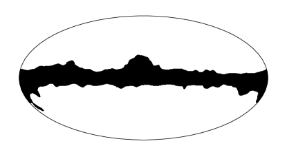
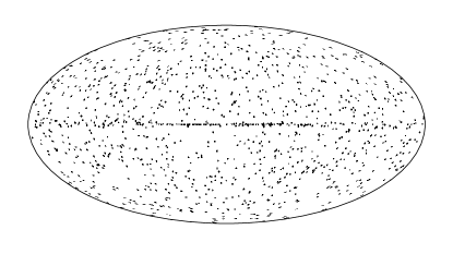
Figure 1: The galactic (left) and point source mask (right) used in Table 2. The galactic mask is the $f_{\mathrm{sky}}=0.80$ galactic mask included in the Planck 2013 release, and the point source mask is the one based on the Planck LFI 30 GHz channel from the 2013 release (with a $4\sigma$ threshold level), which has $f_{\mathrm{sky}}=0.96$. The combined mask has $f_{\mathrm{sky}}=0.77$.

To illustrate quantitatively the problems encountered in determining $f_{\mathrm{NL}}$ with a mask, we applied a series of tests to simulated CMB maps as described in Table 2. The masks used are shown in Fig. 1 while the details of the simulations are described in the caption of the Table. We find that when missing data in the masked regions are naively replaced with the average of the unmasked part of the map (the “no filling in” lines in the Table), the estimates of $f_{\mathrm{NL}}$ are unbiased but have much larger variance than expected, at least in temperature. The expected increase in the standard deviation is only a factor $1/\sqrt{f_{\mathrm{sky}}}$ (i.e., $1.12$ for the galactic mask and $1.02$ for the point sources) and in particular for the point source mask we observe wider error bars in temperature for all three shapes. Including the linear correction term (2.20) in the estimator reduces this effect to some extent, but in temperature this is clearly not enough. The effect of the point source mask on the local shape is exacerbated when the holes are smaller. For example, replacing the 2013 Planck LFI 30 GHz point source mask with the 2013 Planck HFI 100 GHz channel mask (with a $5\sigma$ threshold level), which has a much smaller beam and hence smaller holes ($f_{\mathrm{sky}}=0.99$), increases the “no filling in, no linear correction” error bars for the local shape from 9.2 to 29.5 (while the error bars for equilateral and orthogonal become smaller). These results demonstrate the need for a suitable filling in of the missing data in the masked regions of the temperature map, in particular for the point source mask.

The simplest filling in method is diffusive filling in, which despite its simplicity worked extremely well and was subsequently adopted for the other Planck bispectrum estimators (KSW and modal) as well. It became the common method in both the 2013 and 2015 Planck releases. After filling the masked regions with the average of the unmasked part of the map as above, we fill each masked pixel with the average value of its neighboring pixels and this procedure is iterated. We found that 2000 iterations sufficed for the Planck maps. One can implement the iterative procedure in two different ways: compute the average of the neighbors on the current iteration (Gauss-Seidel method, where some of the neighbor pixels will already have been updated and others not) or on the previous iteration kept in a buffer (Jacobi method, where all neighbor pixels will be on the previous iteration). While the Gauss-Seidel implementation is anisotropic, we found that this has no impact on the results, while on the contrary the faster convergence of that implementation is an advantage. This scheme solves a discretized version of Laplace’s equation for the pixels where there is no data with the boundary of the unmasked region providing Dirichlet boundary data. [See [36] for a discussion of how this scheme is related to constrained random Gaussian realizations for filling in the missing data.] While this sort of ‘harmonic averaging’ is simple to implement and dulls the sharp edges, it appears at first glance not to remedy the problem of missing small-scale power described above, as the resulting maps have clearly visible bald spots, see Fig. 2. However, unlike apodization which only dulls the edges, the diffusive filling in scheme does create small scale structure inside close to the boundary of the mask. Given that during harmonic transforms it is the wavelength of the modes that determines how far they propagate, this is exactly what we need: the short wavelengths can only propagate small distances and hence need only be reconstructed close to the edges. Fig. 3 illustrates both how the contamination due to the presence of the point source mask is localized around the holes and how filling in remedies this problem. We use the Planck HFI 100 GHz point source mask (with the smaller holes) for this Figure, since the effect is larger and more apparent there.

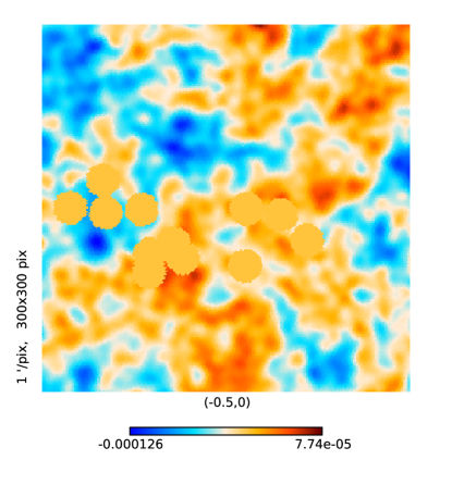
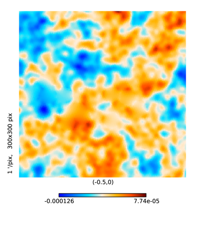
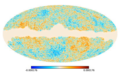
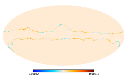
Figure 2: The top two panels show a zoom of a Gaussian CMB map with holes from the 2013 Planck HFI 100 GHz point source mask, before (left) and after diffusive filling in (right) with 2000 iterations. The bottom left panel shows what filling in the galactic mask looks like, with the bottom right panel showing the difference between the maps with and without filling in. The units are dimensionless ($\Delta T/T_{0}$).

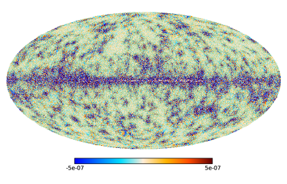
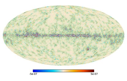
Figure 3: Here we take one of the Gaussian CMB maps and filter out all modes except $\ell\in[1500,1549]$ in three different ways. First we take the unmasked map, filter it, and mask the result (1). Secondly, we take the map, mask it with the 2013 Planck HFI 100 GHz point source mask, then filter it and mask again (2). Finally, the third map (3) is the same as the second one, except that we have performed diffusive filling in on the masked map before filtering. On the left is shown the difference $(2)-(1)$ (no filling in), while on the right we have $(3)-(1)$ (with filling in). The units are dimensionless ($\Delta T/T_{0}$).

After masking, filling in, and filtering the maps, we mask them once again before integrating over products of maps. The masked region is never directly used in the calculation of the bispectrum, but the filling in is crucial to avoid the influence of the masked region spreading out over the sky when filtering the maps, as explained above. In addition the average of the filtered maps outside the mask is subtracted to remove any monopole. If this is not done small-scale power (whose origin is from the two-point function) will combine with this monopole to masquerade as (local) bispectral power, and this ‘aliasing’ can be a large effect.

Other more sophisticated filling in techniques include nonlinear methods based on sparsity (see [37, 38, 39]) or constrained Gaussian realizations [36]. Alternatively, and even better for bispectrum determination, one can perform a full inverse covariance weighting (Wiener filtering) of the maps (see e.g., [40, 41]). However as the results in Table 2 show, these methods do not appear necessary, as a combination of diffusive filling in and the linear correction term leads to results that are effectively optimal for the temperature maps (meaning they cannot be distinguished from the optimal results within the error bars). For $E$ polarization the situation is even simpler, at least at the Planck resolution and sensitivity. Not even diffusive filling in is required. Just applying the linear correction term appears sufficient. However as a precaution we also applied diffusive filling in to the $Q$ and $U$ maps for the Planck analysis.

Table 2 also highlights the importance of the linear correction term when there is anisotropic noise. While there is hardly any impact for the equilateral shape and no bias for any shape, for the local shape the error bars simply explode when we add anisotropic noise to the map, both for temperature and for the $E$ polarization mode. (For an explanation see Section 2.3.) However including the linear correction term described in Section 2.3 suffices to recover the same error bars as in the ideal case. As can be seen from (2.20), the linear correction to the bispectrum of a given map, and hence to the $f_{\mathrm{NL}}$ parameters via (3.24), involves the average over a large number of Gaussian maps. In Fig. 4 we show the histogram of the individual contributions of 199 Gaussian maps to the linear correction part of $f_{\mathrm{NL}}$ for one of the maps from the “no mask, anisotropic noise” case of Table 2. The corresponding mean values are for $T$: local $165\pm 0.5$, equilateral $-4\pm 8$, orthogonal $-40\pm 4$, and for $E$: local $-415\pm 3$, equilateral $-20\pm 24$, orthogonal $119\pm 11$. As expected we see a hugely significant linear correction for local, a very significant correction for orthogonal (due to the large correlation with local), and no significant correction for equilateral. The error bars on the linear correction term for a single map are much smaller (in this case of 199 maps about a factor 7) than the error bars on the values of the different $f_{\mathrm{NL}}$ parameters determined from 100 maps in Table 2, indicating that we have used enough maps to determine the linear correction. Another way of representing the importance of the linear correction term in the presence of anisotropic noise is shown in the scatter plot of Fig. 5.

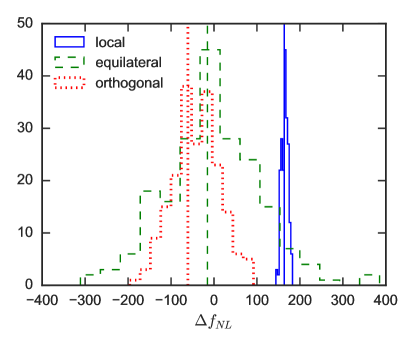
Figure 4: Histogram of the contribution of 199 individual Gaussian maps to the linear correction part of $f_{\mathrm{NL}}$ for one of the maps from the “no mask, anisotropic noise” case of Table 2, for both temperature (left) and $E$ polarization (right). Results are shown for the local (blue), equilateral (green), and orthogonal (red) shapes. The vertical lines correspond to the cubic (uncorrected) part of $f_{\mathrm{NL}}$ for that map.

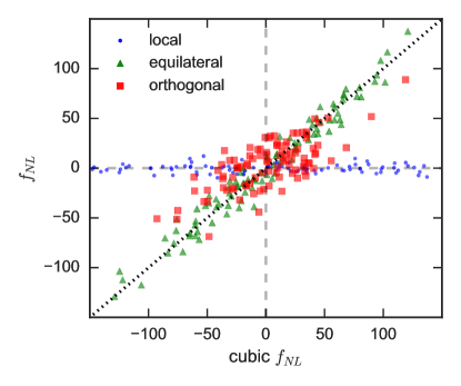
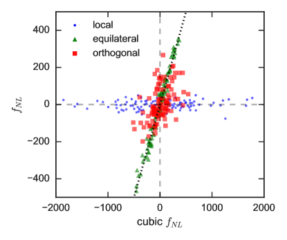
Figure 5: Scatter plot of the values of $f_{\mathrm{NL}}$ without linear correction (horizontal axis) against the values including linear correction (vertical axis), for the 100 maps of the “no mask, anisotropic noise” case of Table 2. Results are shown for temperature (left) and $E$ polarization (right) and for the local (blue), equilateral (green), and orthogonal (red) shapes. We clearly see the huge effect of the linear correction term for the local shape (where a wide range of uncorrected values all map onto a small range of corrected values, without any apparent correlation), some effect for orthogonal, and no effect for equilateral (where the corrected and uncorrected values are very similar and highly correlated).

5 Implementation of the estimator

A significant advantage of the binned bispectrum estimator is that it divides the bispectral analysis and determination of $f_{\mathrm{NL}}$ into three separate parts, the first two of which are completely independent. The first, slow, part is the computation of the raw binned bispectrum of the map under consideration, including its linear correction. The second, much faster, part involves the computation and subsequent binning of the theoretical bispectrum templates one wants to test and of the expected bispectrum covariance. Finally, the third, extremely fast, part (that runs in less than about a minute) is where the different analyses (for example for different templates) are carried out using the raw binned bispectrum from part 1 and the quantities from part 2 as an input. In the case of $f_{\mathrm{NL}}$ determination, this last part corresponds to the evaluation of the sum over the bins and polarization indices in the inner product (3.28) used in (3.24).

This approach has several advantages. Firstly, the full (binned) bispectrum is a natural output of the code and can be studied on its own without a particular template in mind. Such an analysis will be the subject of the last Sections of the paper. Secondly, there is no need for the bispectrum template to be separable, since nowhere in the method does the need arise to split up the template into a separable form. Thirdly, once the bispectrum of a map has been computed, modifications to the theoretical analysis (like for example testing additional templates) is fast, since there is no need to rerun the observational part (which consumes by far the most time). This is in contrast with competing estimators such as the KSW estimator, where the theoretical and observational steps are mixed together (a separation is instead made in terms of $\ell_{1},\ell_{2},\ell_{3}$), so that the full code has to be rerun for any new template. Fourthly, with the binned bispectrum estimator the dependence of $f_{\mathrm{NL}}$ on $\ell$ is obtained almost for free, simply by leaving out bins from the sum when computing the final inner product. In particular this has been used to study the dependence on $\ell_{\mathrm{min}}$ and $\ell_{\mathrm{max}}$ in the Planck analysis. Finally, the binned bispectrum estimator compares favorably to the other estimators in terms of speed: it is very fast on a single map.

The only disadvantage of this method is that the templates that can be studied accurately have to be reasonably smooth, or if not then any rapid changes should be limited to a small part of $\ell$-space, in order for the template to be well approximated by a binned template with a not too large number of bins. For most primordial and foreground templates studied so far, this is not a problem. Moreover, even for templates that do not satisfy this criterion, the binned bispectrum estimator could still perform quite well. For example, among the templates discussed in Sections 3.1.1 and 3.1.2, only the lensing-ISW template cannot be easily binned. For a typical Planck binning the overlap is of the order of 60–70% (as opposed to 95% or higher for all the other templates considered). Nevertheless the binned bispectrum estimator gives unbiased results even for this template, with error bars that are only slightly widened.

The code has been written mainly in Python, using some routines written in C. It is run on the computers of the Centre de Calcul de l’Institut National de Physique Nucléaire et de Physique des Particules (CC-IN2P3) in Lyon, France and any explicit remarks about computing time refer to that system.

5.1 Theoretical part

The theoretical part of the code consists of two steps: first determining the unbinned theoretical bispectrum and power spectrum, and second, computing from these spectra the binned bispectrum templates $B^{\mathrm{th}}_{i_{1}i_{2}i_{3}}$ and the inverse of the binned covariance matrix $(V^{-1})_{i_{1}i_{2}i_{3}}^{p_{1}p_{2}p_{3}p_{4}p_{5}p_{6}}$, see (3.24) and (3.28). This also requires experimental inputs in the form of the beam transfer function $b_{\ell}$ and the noise power spectrum $N_{\ell}$.

The first step is in some sense not really part of the estimator code. We have a code to compute all the bispectra discussed in Sections 3.1.1 and 3.1.2, but in principle an explicitly computed theoretical bispectrum from any source could be used here. In our code we use the radiation transfer functions $\Delta_{\ell}^{p\,I}$ (with $p$ the polarization index and $I$ the isocurvature index) computed with CAMB (slightly modified to write them to file, since these are not a normal output of CAMB) to compute the primordial templates (3.2). For separable templates, this is a fast calculation, since the triple integral over $k_{1},k_{2},k_{3}$ becomes a product of single integrals. For non-separable templates a brute force calculation is much slower, but while one might look for smarter ways to compute such bispectrum templates, it should not be forgotten that (for a given cosmology) for use in the binned bispectrum estimator, a template has to be computed only once. Hence even a slow calculation might be acceptable. While this code can also compute the power spectra from the radiation transfer functions according to (3.1), in practice we use the power spectra computed by CAMB. These power spectra are used in the covariance matrix and some foreground bispectrum templates. This code is similar to the code described in [7], except for the inclusion of additional primordial templates and the generalization to polarization and isocurvature. Since the calculation of the $N_{\triangle}^{\ell_{1}\ell_{2}\ell_{3}}$ in real time is fast enough, these are no longer precomputed and stored. The primordial bispectra are precomputed only on a grid (with $\Delta\ell$ increasing to about 10 at high $\ell$). This is denser than the binning, and thus accurate enough for the smooth local, equilateral, and orthogonal templates.

The second step involves the binning of the bispectrum templates and the covariance matrix. The calculation of the covariance matrix from the power spectra as well as the calculation of the foreground templates is done directly in this step. As was seen in Section 3.1.1, the foreground templates are simpler to compute than the primordial templates, since there are no integrals, so there is no need to precompute them, the required values can be computed in real time while binning. As for the precomputed primordial templates, since these have been precomputed only on a grid, other values are computed by three-dimensional linear interpolation. While we developed a tetrahedral integration scheme to speed up the calculation of all binned quantities, as described in [7], recently we have moved away from using it. Given that the theoretical computation is much faster than the observational computation, there is no point in making additional approximations to speed it up. Performing an exact calculation of the binned quantities (where the quantities are explicitly computed for each value of $\ell_{1},\ell_{2},\ell_{3}$ and then summed over the bin) is fast enough. We can thus also directly compute the overlap between the binned and the exact template using (3.29).

The final output of this step consists of two files: one containing the binned theoretical bispectrum for all requested shapes, polarization and isocurvature components; and another containing the inverse of the binned covariance matrix for all polarization components. In addition the exact Fisher matrix (3.35) (without binning) is produced to allow for the estimation of the accuracy of the binning approximation using (3.29).

5.2 Choice of binning

The choice of binning is an important part of the implementation. In theory the idea is very simple: one chooses the binning that makes the overlap parameter $R$ defined in (3.29) as close to one as possible. In practice this is not so simple, since both the number of bins and all the bin boundaries are free parameters. Fortunately $R$ does not depend strongly on the exact binning choice. Moreover, one does not need $R=1$ to obtain results statistically indistinguishable from the exactly optimal results. For example, even with $R=0.95$, which is about the lowest overlap for any of the templates considered in the Planck analysis (except for lensing-ISW), the increase in the standard deviation is only 2.6%. This should be compared to the 5% uncertainty in the standard deviation due to its determination from 200 maps. Note that the code allows the use of separate binnings for the $T$-only, the $E$-only, and the full $T+E$ analyses, although for reasons related to time a single binning was used for the Planck analysis.

We developed three optimization tools: one that checks which bin boundary can be removed with the smallest decrease of $R$ (reducing the number of bins by one), one that checks where a bin boundary can be added with the largest increase in $R$ (increasing the number of bins by one; the bin boundary is added in the exact center of an existing bin), and one that tries moving all the bin boundaries by a given amount (relative to the size of the bin) and tells for which bin this increases $R$ the most (leaving the number of bins unchanged). For all of them one can indicate which shapes and polarizations (meaning $T$ and/or $E$) should be taken into account. These three tools are then used iteratively to optimize the binning used as starting point, until no more significant improvements are obtained (as defined by a certain threshold in the change of $R$). The starting point is arbitrary. For example a simple log-linear binning (with bin sizes increasing logarithmically at low $\ell$, up to a certain value of $\ell$, after which the binning becomes linear) or a binning that has already been partially optimized in another way can be used. The latter could for example be done using the method described in [7], which can provide a good starting point. (That method produces suboptimal binnings and can benefit significantly from the procedure described here.) While this method can likely be optimized further, for the Planck analysis the binning obtained in this way produces effectively optimal results.

5.3 Observational part

The observational component of the code consists of two parts: one to compute the cubic part of the bispectrum of the map according to (2.7), and the other to compute the linear correction according to (2.20). First the map is fully prepared, which can be as simple as reading an existing map and doing the masking and filling in, or involve the creation of CMB and noise realizations. It is then saved in the form of $a_{\ell m}$’s for later use with the linear correction term, or for reproducibility in the case of generated random realizations.

The maps are then filtered according to (2.6). This leads to some practical issues that had to be resolved, since in principle we need to hold twice ($T$ and $E$) 50–60 maps (one for each bin) of Planck resolution ($n_{\mathrm{side}}=2048$) in memory for this calculation. However our computer system has a limit of 16 GB per processor, which makes this impossible. We managed to save space in two ways. In the first place, while all the preprocessing of the maps is done in double precision, the final filtered maps are only kept in single precision, which saves a factor two in memory. Tests have shown that this has no significant impact on the final result for $f_{\mathrm{NL}}$. Secondly, it is unnecessary to use $n_{\mathrm{side}}=2048$ precision for the maps that contain only low-$\ell$ bins. Hence the filtered maps of bins up to about $\ell=800$ are produced at $n_{\mathrm{side}}=1024$, which saves a factor of four in memory for those maps (the number of pixels in the map is $12\,n_{\mathrm{side}}^{2}$), as well as speeding up the final computation where three maps have to be multiplied and summed (see (2.7)). Using the nested Healpix format, it is easy to multiply maps of different $n_{\mathrm{side}}$ together.

We have developed two different ways of computing the linear correction term of a map. In the first method, which was used for the Planck analysis and the analyses for this paper, each job treats one of the Gaussian maps (see (2.20)), which is preprocessed and filtered as above, and the filtered maps are held in memory. Then a filtered map of only the first bin of the observed map is created and all required sums of products involving that map are computed. Next this process is repeated for the second bin of the observed map, etc. The final result of this job is a temporary file with a linear correction term computed with just one Gaussian map. Once all jobs have finished (with the results for the other Gaussian maps), the results are summed and averaged to obtain the final linear correction term for the map. This whole process (preprocessing the map and computing the cubic and linear terms) for a single map at Planck resolution for all $T+E$ (including mixed) components takes a few hours, which is quite fast compared to other bispectrum estimators. (Computing the theoretical part is much faster and requires only a single job, so can easily be done on the side.) With this method one can simply add more Gaussian maps to the linear correction term at a later stage if required, and investigate its convergence as a function of the number of Gaussian maps. However, this first method of computing the linear correction term scales very badly with the number of observed maps. Since the object $\langle M_{i_{1}}^{p_{1},G}M_{i_{2}}^{p_{2},G}\rangle$ in (2.20) is too large to compute directly and save to file, if one has a set of similar maps (for example to compute error bars), the linear correction term has to be recomputed for each map in the same way as above, making this a very slow process.

For this reason we recently developed another way to compute the linear correction term. This second method is based on the observation that while the object $\langle M_{i_{1}}^{p_{1},G}M_{i_{2}}^{p_{2},G}\rangle$ (consisting of 6612 maps for a full $T+E$ calculation in the case of 57 bins) is too large to handle, saving it in the form of $a_{\ell m}$’s is doable. Moreover, we make use of the fact that when multiplying several masked maps together (all with the same mask), it is enough if only one of the maps is masked. Hence if the observed map in (2.20) is properly masked, the Gaussian maps can be left unmasked (since the Gaussian maps are based on simulations, they are full-sky maps). This has the advantage that no filling-in needs to be performed on these maps, which would otherwise be required before conversion to $a_{\ell m}$’s, as explained in section 4. By limiting the number of considered bins per job in such a way that both the filtered maps for those bins and all the product maps involving those bins can be kept in memory at the same time, one job can compute the full average for the considered bins by treating one Gaussian map after the other. Only at the end are the final maps converted to $a_{\ell m}$ format and written to disk. This precomputation for the linear correction term can be run with a modest number of jobs (about 100) in a reasonable amount of time (less than a day for 200 maps). Once the precomputation has finished, the linear correction for any map can be quickly computed using (2.20). Each job reads in a number of product maps (i.e. for certain values of $i_{1}$ and $i_{2}$; the number being determined by memory considerations), and converts them back to pixel space. They are then multiplied with the filtered observed maps as explained above for the first method. The main difference is that the results are now for the full average of all the Gaussian maps, instead of for a single one. Another (small) advantage of this second method is that at this step we only need to multiply two maps together and not three. Once all jobs are finished, the temporary files containing results for different $i_{1}$-$i_{2}$ bins are combined to get the full linear correction for the observed maps. While this second method with precomputation is slower if one is only interested in a single map, its much better scaling with the number of maps makes it by far the preferred method when dealing with a set of maps, for example to compute error bars.

The final result of this part are two files for each map, one containing the binned cubic-only bispectrum of the map and the second its linear correction, both containing all requested polarization components. These can then be combined with the results from the theoretical part to compute $f_{\mathrm{NL}}$ according to (3.24), which takes less than a minute even when producing convergence plots and dependence on $\ell$ as well, or be studied directly without the assumption of a theoretical template, as discussed in Section 6.

6 Smoothed binned bispectrum

The previous Sections described how the binned bispectrum of a map can be analysed parametrically by computing the $f_{\mathrm{NL}}$ parameters corresponding to a selection of theoretically motivated templates. But one advantage of the binned bispectrum estimator is that the full (binned) three-dimensional bispectrum is a direct output of the code, which can be studied non-parametrically, thus searching for any deviations from Gaussianity even when no suitable template is available. Here we describe the smoothing procedure that must first be applied to the binned bispectrum in order to enhance the signal-to-noise of any possible non-Gaussian features, which otherwise would remain hidden in the noise. The next Section describes the statistical analysis subsequently applied to this smoothed binned bispectrum to assess the statistical significance of any non-Gaussian features appearing as extreme values.

We first normalize the binned data by dividing by the square root of the expected bin variance, so that each bin triplet in the absence of a bispectral signal would have noise obeying a normalized Gaussian distribution. Thus for the bin triplets for which there is data, we define

$${\cal B}_{i_{1}i_{2}i_{3}}^{TTT}=\frac{B_{i_{1}i_{2}i_{3}}^{TTT}}{\sqrt{V_{i_{1}i_{2}i_{3}}^{TTTTTT}}},\qquad{\cal B}_{i_{1}i_{2}i_{3}}^{EEE}=\frac{B_{i_{1}i_{2}i_{3}}^{EEE}}{\sqrt{V_{i_{1}i_{2}i_{3}}^{EEEEEE}}},$$

$${\cal B}_{i_{1}i_{2}i_{3}}^{T2E}=\frac{B_{i_{1}i_{2}i_{3}}^{T2E}}{\sqrt{\mathrm{Var}(B^{T2E})_{i_{1}i_{2}i_{3}}}},\qquad{\cal B}_{i_{1}i_{2}i_{3}}^{TE2}=\frac{B_{i_{1}i_{2}i_{3}}^{TE2}}{\sqrt{\mathrm{Var}(B^{TE2})_{i_{1}i_{2}i_{3}}}}.$$ (6.1)

For the mixed $T$ and $E$ components we analyzed only the combinations $B^{T2E}\equiv TTE+TET+ETT$ and $B^{TE2}\equiv TEE+ETE+EET$, with corresponding variance Var($B^{T2E}$) = Var($TTE$) + Var($TET$) + Var($ETT$) + 2 Cov($TTE,TET$) + 2 Cov($TTE,ETT$) + 2 Cov($TET,ETT$), and similarly for Var($B^{TE2}$). This projection entails a loss of information but allows the same analysis to be used as for $TTT$, as described below. Results for the unsymmetrized mixed bispectra will be discussed in a future publication.

As discussed in Section 2.1, only bin triplets containing $\ell$’s that satisfy both the parity condition and the triangle inequality contain data. However, among the bin triplets containing data, we noticed that some triplets systematically produced outliers. It turned out that these bin triplets contained very few valid $\ell$-triplets [for example, the hypothetical bin triplet $([50,100],[50,100],[200,300])$ would contain only one valid $\ell$-triplet (100,100,200), since the triangle inequality imposes that $l_{3}\leq l_{1}+l_{2}$]. While the theoretical variance calculation is exact, the computation of the observed bispectrum using Healpix spherical harmonic transforms contains some numerical inaccuracies, so that the bispectrum in points outside the triangle inequality is not zero but contains leakage. For bin triplets like the above example with many $\ell$-triplets violating the triangle inequality, a significant mismatch between the theoretical and the actual standard deviation of the bispectrum in that bin is observed. The obvious solution is to remove such bin triplets from the data. Moreover, the statistical analysis described in the next Section assumes that bin triplets contain many valid $\ell$-triplets in order for Gaussian statistics to apply to the noise from cosmic variance, which constitutes another reason to exclude such triplets. After some experimentation, we adopted the selection criterion that the ratio of valid $\ell$-triplets to the ones satisfying only the parity condition (but not the triangle inequality) in a bin triplet should be at least 1%, finding this a good threshold for rejecting systematic outliers. The results are insensitive to the precise threshold used. For the Planck binning with 57 bins (which is used for the results in this Section and the next), this criterion excluded 293 out of 13020 bin triplets.

If we were looking for a sharp bispectral feature of a linewidth narrow compared to the binwidth, there would be no motivation to smooth. We would simply examine the statistical significance of the extreme values of the renormalized binned bispectrum described above taking into account the look elsewhere effect. However for broad features, as are likely to arise from galactic foregrounds, smoothing increases statistical significance by averaging over and thus diminishing the noise. One approach would be to use binning with a range of bin widths, but this approach has the disadvantage that the statistical significance for detecting a feature depends on how it is situated relative to the neighbouring bin boundaries. Instead we rather smooth using a Gaussian kernel and renormalize so that in the absence of a signal the single pixel distribution function is again a unit Gaussian. For a Gaussian kernel $K_{\sigma_{\mathrm{bin}}}$ of width $\sigma_{\mathrm{bin}}$, we have

$$\mathcal{B}^{p_{1}p_{2}p_{3},\text{smoothed}}_{i_{1}i_{2}i_{3}}=\sum_{i^{\prime}_{1}}\sum_{i^{\prime}_{2}}\sum_{i^{\prime}_{3}}K_{\sigma_{\text{bin}}}(i_{1}-i^{\prime}_{1},i_{2}-i^{\prime}_{2},i_{3}-i^{\prime}_{3})\mathcal{B}^{p_{1}p_{2}p_{3}}_{i^{\prime}_{1}i^{\prime}_{2}i^{\prime}_{3}}$$ (6.2)

where the Gaussian smoothing kernel

$$K_{\sigma_{\text{bin}}}(\Delta i_{1},\Delta i_{2},\Delta i_{3})=\left(2\pi{\sigma_{\mathrm{bin}}}^{2}\right)^{-3/2}~{}\exp\left[-\frac{1}{2}\frac{{\Delta i_{1}}^{2}+{\Delta i_{2}}^{2}+{\Delta i_{3}}^{2}}{{\sigma_{\mathrm{bin}}}^{2}}\right]$$ (6.3)

is used. Numerically the kernel is applied in the Fourier domain.

Without boundaries this smoothing and renormalization procedure would be straightforward. However near the boundary the Gaussian smoothing kernel would extend into the region where there is no data. To minimize boundary effects, we first extend the fundamental domain (where $i_{1}\leq i_{2}\leq i_{3}$) to the five identical domains obtained by permuting $(i_{1},i_{2},i_{3})$ and pad with zero data beyond the boundaries of this extended domain as well as for triplets inside the domain for which there is no data. The smoothing causes power to leak out into the zero padded regions, and to correct for this leakage, we construct a mask consisting of ones in the domain of definition and zeros outside. After smoothing the signal-to-noise bispectrum $\mathcal{B}$, we renormalize by dividing by the mask that has undergone the same smoothing procedure. For the bin triplet statistic to be a Gaussian of unit variance, we generate 1000 Monte Carlo realizations going through the same procedure and compute the variance, with which we divide our smoothed renormalized bispectrum.

The result using different smoothing lengths is illustrated in Fig. 6 as two-dimensional slices showing $\mathcal{B}$ as a function of $\ell_{1}$ and $\ell_{2}$ for a fixed bin in $\ell_{3}$. As a further illustration, to show what certain known non-Gaussian features look like in this representation, we present in Appendix A slices of the smoothed theoretical template bispectra from Sections 3.1.1 and 3.1.2. With the color scale used in Fig. 6, both dark red and dark blue represent extreme values with small $p$ values if Gaussianity is assumed, and thus suggest the presence of statistically significant bispectral non-Gaussianity. A correct analysis of the significance would also take into account the look elsewhere effect — that is, that the small probability to exceed, calculated for a fixed bin, is too small because it does not reflect that an improbable value could have occured in any of a number of bins. The analysis of this issue is complicated by the correlations between the bins that result from the smoothing, an issue analyzed in the next Section.

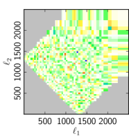
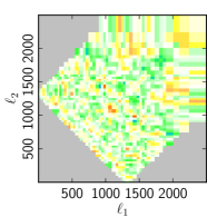
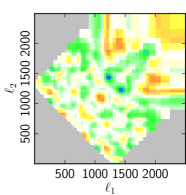
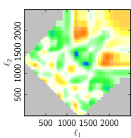
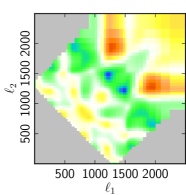
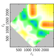
Figure 6: Effect of different smoothing lengths on the bispectrum of one of the Gaussian maps from Table 2 with galactic and point source masks and anisotropic noise. From left to right and top to bottom are shown: no smoothing, smoothing using $\sigma_{\mathrm{bin}}=$ 0.5, 1, 1.5, 2, 2.5 and 3. The slices correspond to $\ell_{3}\in[1291,1345]$.

7 Statistical analysis

This Section addresses how to assess the statistical significance of possible bispectral non-Gaussianity in the binned bispectrum that has been smoothed according to the procedure described in the previous Section. Even in the case of a Gaussian sky, where before the smoothing over bins has been applied the single-bin distribution function is a normalized Gaussian for which the values in distinct bins are statistically independent, after this smoothing procedure fluctuations in neighboring bins become correlated, complicating the analysis. We consider here how to deal with this complication.

In the absence of smoothing, we face the following statistical problem. We have a binned bispectrum that has been rescaled so that we have $N$ bins and the bispectrum value in each bin $x_{i},$ where $i=1,\ldots,N$, has a probability distribution function well approximated by a normalized Gaussian distribution. Moreover, values in different bins are almost statistically independent. The quadratic correlation vanishes, but some of the higher order joint correlations do not precisely vanish, a feature that we shall neglect here. The corrections to Gaussianity and to statistical independence are suppressed when $\ell$ is large and when there are many $\ell$-triplets containing data in a bin. Thus we have the distribution function

$$p(x_{1},\ldots,x_{N})=(2\pi)^{-N/2}~{}\exp\left[-\frac{1}{2}\sum_{i=1}^{N}{x_{i}}^{2}\right],$$ (7.1)

and since we are interested in extreme values, we define two new derived statistics

$$X_{\mathrm{min}}=\min(x_{1},\ldots,x_{N});\qquad X_{\mathrm{max}}=\max(x_{1},\ldots,x_{N}),$$ (7.2)

and accordingly define the $p$-values

$$p_{\mathrm{min}}(X)=P(X_{\mathrm{min}}<X);\qquad p_{\mathrm{max}}(X)=P(X_{\mathrm{max}}>X)$$ (7.3)

where $X_{\mathrm{min}}$ and $X_{\mathrm{max}}$ are the derived random variables defined above. If either of these $p$-values are extremely small, then we have evidence of bispectral non-Gaussianity directly in the unsmoothed binned bispectrum, and this $p$-value can be converted into a $\sigma$ for the normal distribution using the inverse error function as is customary.

For this simple unsmoothed case it is not hard to give the probability distribution function for the extreme value statistics $X_{\mathrm{min}}$ and $X_{\mathrm{max}}$. Given the (complementary) cumulative distribution function for the normal distribution (integrating from right to left)

$$\Phi(x)=\frac{1}{\sqrt{2\pi}}\int_{x}^{+\infty}dt~{}\exp\left[-\frac{1}{2}t^{2}\right],$$ (7.4)

the analogous distribution for the maximum extreme value for $N$ variates is given by

$$\Phi_{\mathrm{max}}(X_{\mathrm{max}};N)=1-\Bigl{(}1-\Phi(X_{\mathrm{max}})\Bigr{)}^{N}$$ (7.5)

and we may straightforwardly obtain an analogous expression for the case of the minimum value. (Below we shall only give results for the case of the maximum.) For $X\gg 1$ we obtain an approximation to $\Phi_{\mathrm{max}}(X_{\mathrm{max}};N)$ by inserting the following expression [42]

$$\ln\Bigl{[}\Phi(X)\Bigr{]}\approx-\left[\frac{X^{2}}{2}+\ln(X)+\frac{1}{2}\ln(2\pi)\right]$$ (7.6)

into (7.5).

When we consider extreme values of multivariate Gaussian distributions with correlations, there is, as far as we know, no way of obtaining an analytic result for the extreme value distribution for $\Phi_{\mathrm{max}}(X_{\mathrm{max}})$. After the smoothing described in the previous Section is applied, the probability distribution defined in (7.1) must be replaced with

$$p({\bf x})=(2\pi)^{-N/2}~{}\exp\left[-\frac{1}{2}{\bf x}^{T}{\bf C}~{}{\bf x}\right]$$ (7.7)

where the correlation matrix ${\bf C}$ has all ones on the diagonal, but also a lot of positive off-diagonal elements as the result of the smoothing process, rather than all zeros away from the diagonal. It is these off-diagonal elements that prevent us from solving analytically for the extreme value statistic probability distribution function.

Instead we postulate an Ansatz to approximate the cumulative distribution function (CDF) of the extreme value statistic $\Phi_{\mathrm{max}}$, which has one adjustable parameter $N_{\mathrm{eff}}$, the effective number of independent bins, which will be smaller than the actual number of bins $N$ as the result of the smoothing. The Ansatz states that the CDF given in (7.5) [and approximated using (7.6)] holds where $N$ has been replaced with $N_{\mathrm{eff}}$. For a given level of smoothing, we fit $N_{\mathrm{eff}}$ to the tail of the CDF, which has been determined empirically by Monte Carlo simulations. We then assess the quality of the approximation, in particular in the tail of the distribution where $X$ is very large, which is the range of values of particular interest here. It should be stressed that we do not need a good approximation to the entire CDF. It suffices to have an approximation that works well asymptotically, in the extreme tail of the distribution where $p$-values cannot feasibly be obtained by Monte Carlo methods. Thus the Ansatz serves as an asymptotic approximation for the tail of the distribution.

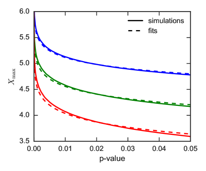
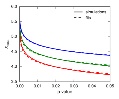
Figure 7: Fitting the extreme values of the smoothed bispectrum. The horizontal axis gives the $p$-value and the vertical axis the maximum bin deviation in number of $\sigma$. The solid curves show the CDFs for the smoothed $64^{3}$ cubes (figure on the left) for $\sigma_{\mathrm{smoothing}}=2,5,$ and $10$ (respectively from top to bottom blue, green and red) and for the more realistic situation (figure on the right) for $\sigma_{\mathrm{smoothing}}=1,2,$ and $3$ as described in the main text. We show only the 5% most extreme values, since we are interested in the extreme tail of the distribution. The dashed curves show non-linear least square fits to these curves using the Ansatz where a distribution with a smaller number $N_{\mathrm{eff}}$ degrees of freedom is used to approximate the distribution with correlations between bins. Here (from top to bottom in the figure on the left) $N_{\mathrm{eff}}=61900,3709,$ and $351$ are used to represent the $64^{3}=2.6\times 10^{5}$ degrees of freedom with various degrees of correlation as the result of the smoothing (see the main text for the values of the figure on the right). The fit provides a good approximation, especially at the small $p$-values that are of the greatest interest for this application.

To demonstrate the validity of our Ansatz in a simplified context very similar to the case of interest, we generate a three-dimensional periodic cubic lattice filled with $64^{3}$ independent realizations of a normal Gaussian random variable. This cube is then smoothed using a Gaussian smoothing kernel with widths $\sigma_{\mathrm{smoothing}}=2,5,$ and $10$. The smoothed cube is rescaled so that the variable at each lattice point has unit variance. For each smoothing width, the extreme value statistic (maximum) is taken for $10^{6}$ realizations and only the greatest $5\%$ of the extreme values are retained. Fig. 7 (left) shows the empirical CDF for the extreme values, which are compared to the functional form of the Ansatz for the best-fit values of $N_{\mathrm{eff}}$ according to the approximation given in (7.6).

The above discussion demonstrates that an extreme value distribution for $N_{\mathrm{eff}}$ independent Gaussian variates can be used to approximate the distribution for $N_{\mathrm{bin}}$ variates with correlations due to smoothing. However, the geometry of the allowed bins is complicated and must be taken into account. Thus simulations must be carried out to determine $N_{\mathrm{eff}}$ for a given smoothing scale in the more realistic case of the actual bins used for the bispectrum analysis. We show that the Ansatz is still a good approximation also in this case in Fig. 7 (right). We generate random numbers in the domain of definition of the binned bispectrum, and smooth it as for the real data. Restricting to those bin triplets that contain enough valid data (see the discussion in Section 6), these simulations are a good approximation to a Gaussian CMB map’s bispectrum.

We now illustrate this method by applying it to a realistic situation. We add a point source map to a simulated Gaussian CMB map with anisotropic noise, generated as described in the caption of Table 2. The point source simulation was created with the Planck Sky Model, at 143 GHz, with a beam with a FWHM of 5 arcmin, and contains faint infrared sources, as described in [43], and faint radio sources with the improved parameters described in [44]. The galactic and point source masks were applied as described in Section 4.

The binned bispectrum of this map was evaluated applying the linear correction and the filling in procedure, and the $f_{\rm NL}$’s were determined individually for each of the templates described in Section 3.1.1. The unclustered point source contribution was detected with high significance in this contaminated map: $b_{\rm ps}=(64.8\pm 0.8)\times 10^{-29}$. This signal is much stronger than the one detected in the cleaned Planck maps, but of the same order of magnitude as the forecast at 217 GHz (see [5]). No statistically significant detection of a nonzero $f_{\rm NL}$ was obtained for the other templates, with the exception of the CIB template. But the CIB bispectrum has significant overlap with the unclustered point source bispectrum (see Table 1), so this result is not surprising. The nonzero result for $b_{\mathrm{CIB}}$ disappears in a joint analysis of the unclustered point source and CIB templates. Finally we smooth the bispectrum with a few different values of the smoothing length, namely $\sigma_{\rm smoothing}=1,2,3$.

Apart from studying the contaminated bispectrum, we can also try to remove the estimated point source contribution from the measured binned bispectrum, simply by subtracting the corresponding smoothed template (3.6) with the measured amplitude. We can then check if there are remaining non-Gaussian features in this cleaned bispectrum using the method described above. Table 3 gives the maximum bin values for the bispectrum before and after the template cleaning is applied. The minima are not given because the inclusion of the point sources tends to gives a positive bispectral contribution. The $p$-values were calculated using simulations of $10^{6}$ Gaussian realizations and fitting the CDF for $N_{\mathrm{eff}}$ to the empirical distribution. We found that the smoothing lengths $\sigma_{\mathrm{smoothing}}=1,2,$ and $3$ correspond to $N_{\mathrm{eff}}=8664,1948,$ and $588$ respectively. We see that a highly statistically significant detection is found using the above procedure on the uncleaned bispectrum. We also observe that the template cleaning procedure is successful; however, some detectable unsubtracted residual remains. This residual, however, has little overlap with the known theoretically motivated primordial templates.

Smoothing	Before		After
length	template cleaning		template cleaning
($\sigma_{\mathrm{smoothing}}$)	$X_{max}$	$p$-value	$X_{max}$	$p$-value
1	33.4	$e^{-553}$	5.1	$1.5\times 10^{-3}$
2	51.2	$e^{-1308}$	3.6	0.15
3	59.2	$e^{-1751}$	4.4	$3.3\times 10^{-3}$

Table 3: Maximum bin values and associated $p$-values for the bispectrum of a simulated Gaussian CMB + point sources map before and after cleaning of the point source contribution, for various values of the smoothing length. See main text for a more detailed explanation.

8 Conclusions

This paper gives a detailed description of the binned bispectrum estimator, which is one of the three estimators used for the official 2013 and 2015 Planck analyses. The estimator determines the full three-dimensional bispectrum of a map, binned in harmonic space. This binned bispectrum can then be combined with a library of theoretical bispectrum templates to determine the so-called $f_{\mathrm{NL}}$ parameters. This aspect of the binned bispectrum estimator was first described in [7], but many new developements took place since that paper was published and are detailed here. These include the treatment of the masked sky using diffusive filling in, a method which was subsequently adopted by the other bispectrum estimators, and the generalization to include polarization. The binned bispectrum estimator code is fast, has a convenient modular structure, separability of the templates is not required, and the dependence of $f_{\mathrm{NL}}$ on $\ell$ is obtained automatically, thus providing additional information.

Moreover, the binned bispectrum of the map can also be used directly for non-parametric (blind) non-Gaussianity searches. This is useful to investigate the non-Gaussianity of those foregrounds for which there is no theoretically motivated template, or to check for any non-Gaussian primordial signal in a cleaned map beyond the standard templates. For this purpose the binned bispectrum is first smoothed with a Gaussian kernel to increase the statistical significance of any broad features and make them stand out above the noise. The smoothing complicates the statistical analysis of the significance of non-Gaussian features by introducing correlations between neighbouring bins. In this paper we described how to address this complication using approximated extreme value statistics. We illustrated this procedure on the bispectrum of a realistic map that contains a Gaussian CMB and radio point sources, both before and after cleaning the bispectrum with the point source template.

Further applications of the binned bispectrum estimator can be found in the Planck analyses of 2013 [4] and 2015 [5]. In those papers we determined the $f_{\mathrm{NL}}$ values for various theoretical templates, and showed the full smoothed binned bispectrum of the cleaned Planck sky map. A statistical analysis of the Planck smoothed bispectrum according to the method described here will be given in the next Planck release. Applications of the binned bispectrum estimator to foreground maps in order to determine their smoothed bispectra and characterize their non-Gaussianities are planned for a future paper. These bispectra can then be used as templates in a parametric estimation to investigate if contamination remains in cleaned maps.

To conclude we add some comments regarding the possibility of extending our binned estimator methodology to the trispectrum. The reduced trispectrum depends on five scalar variables, which we can represent in the following way. First there are the lengths of the sides of the quadrilateral $\ell_{1}$, $\ell_{2}$, $\ell_{3}$, and $\ell_{4}$. Since the quadrilateral must close, we can write (in the flat-sky approximation for simplicity): $\boldsymbol{\ell}_{1}+\boldsymbol{\ell}_{2}+\boldsymbol{\ell}_{3}+\boldsymbol{\ell}_{4}=\boldsymbol{0}$. But unlike in the case of a triangle, for which the lengths of the sides create a rigid polygon with all angles between the sides determined, for the quadrilateral an ‘internal brace’ is needed to render it rigid. We must additionally specify one more parameter, which we could for example take to be $\ell_{12}=|\boldsymbol{\ell}_{1}+\boldsymbol{\ell}_{2}|$, and now the quadrilateral would be completely rigid, at least in the two-dimensional context that is of interest here. To generalize the technique using filtered maps developed in this paper for the bispectrum to the trispectrum, we cannot simply multiply four filtered maps and take the average. We must, with the parameterization used above for the trispectrum, after taking the products of the filtered $\ell_{1}$ and $\ell_{2}$ maps, apply the $\ell_{12}$ filter before multiplying by the filtered $\ell_{3}$ and $\ell_{4}$ maps, and then take the average in the final step. In other words, writing $F_{1}$ to indicate filtering with respect to the $\ell_{1}$ bin, etc., and $M$ for the CMB map:

$$\mathrm{Trispectrum}_{i_{1}i_{2}i_{3}i_{4}i_{12}}=\int d\hat{\Omega}\,F_{12}(F_{1}(M)F_{2}(M))F_{3}(M)F_{4}(M).$$ (8.1)

This extension will be explored in a future paper.

Acknowledgements: We thank Ata Karakci for providing the simulated radio point source maps generated using the Planck Sky Model, Guillaume Patanchon for useful discussions, and Franz Elsner for useful remarks regarding the lensing-ISW template. The Planck non-Gaussianity working group, in particular the estimator subgroup consisting of James Fergusson, Michele Liguori, Alessandro Renzi, and BvT, provided a stimulating environment for estimator development. We acknowledge the use of the CAMB (http://camb.info) and Healpy (Python version of HEALPix [45]) software packages. We gratefully acknowledge the IN2P3 Computer Centre (http://cc.in2p3.fr) for providing computing resources. BR acknowledges funding from the French Ministère de l’enseignement supérieur et de la recherche and from the Research Council of Norway.

Appendix A Two-dimensional sections of the smoothed theoretical bispectra

To illustrate the smoothed signal-to-noise bispectrum $\mathcal{B}$ that we introduced in Section 6 and to show what certain known types of non-Gaussianity look like, we present here slices of the theoretical template bispectra that we discussed in Sections 3.1.1 and 3.1.2. In Fig. 8 we show the normalized smoothed templates (with smoothing length $\sigma_{\mathrm{bin}}=2$) for six theoretical shapes: local, equilateral, orthogonal, lensing-ISW, unclustered point sources, and CIB (clustered) point sources. All are shown both for $TTT$ and $EEE$, except the point source templates which are $TTT$-only, and for two different slices: $\ell_{3}\in$ [700, 741] and $\ell_{3}\in$ [1291, 1345]. The templates have been normalized with the expected standard deviation assuming the standard Planck cosmology and the same noise and beam properties as in Section 4. Moreover, the templates have been multiplied by such values of $f_{\mathrm{NL}}$ as would lead to a $30\sigma$ detection given those noise and beam properties. Obviously that means different values of $f_{\mathrm{NL}}$ for each template as they all have different error bars. Explicitly these error bars $\sigma_{f_{\mathrm{NL}}}$ are for $TTT$: local 4.7, equilateral 61, orthogonal 32, lensing-ISW 0.21, unclustered point sources $7.0\times 10^{-30}$, CIB point sources $3.6\times 10^{-28}$; and for $EEE$: local 24, equilateral 178, orthogonal 95, lensing-ISW 3.0.

In the three primordial templates, we see the bispectral acoustic oscillations. For the local shape, as expected, the signal is peaked in the squeezed limit (i.e., for a small $\ell_{1}$ and a large $\ell_{2}$ and $\ell_{3}$). The equilateral shape, on the other hand, is peaked for configurations where all $\ell$’s are equal, although that is difficult to see in these Figures since they show just one bin in $\ell_{3}$ and the value is also modulated by the acoustic oscillations. The orthogonal shape explores configurations in the equilateral and flattened ($\ell_{1}+\ell_{2}\approx\ell_{3}$ with $\ell_{1}\approx\ell_{2}$) domains, the latter being visible in the Figures, although again modulated by the acoustic oscillations. We also see its anti-correlation with the local shape (see Table 1). The lensing-ISW signal is highly concentrated in the squeezed limit, and hence has a large correlation with the local shape. The point source templates are featureless and the statistical weight is concentrated for configurations where all three $\ell$’s are large.

Figs. 9 and 10 show the isocurvature templates discussed in Section 3.1.2. Considering only the adiabatic mode together with one isocurvature mode (for which we take consecutively cold dark matter density isocurvature, neutrino density isocurvature, and neutrino velocity isocurvature) gives six independent bispectrum templates. These are denoted respectively by $aaa$, $aai$, $aii$, $iaa$, $iai$, and $iii$ with $a$ for adiabatic and $i$ for isocurvature (see Section 3.1.2 for more details). Since the pure adiabatic $aaa$ template is just the standard local template from Fig. 8, it is not shown here again. The other five templates correspond to one row in the Figures. The different rows then correspond to the different isocurvature modes and different polarization components, as explained in the captions. The difference between the two Figures is the choice of bin for $\ell_{3}$.

Since we want to show the relative size of these templates, we use a normalization different from the first Figure. The smoothed bispectra are still normalized with the same expected standard deviation as before, but they all have $f_{\mathrm{NL}}=1$. Hence their signal-to-noise ratios are all very small and vary a lot from one template to another, so we have chosen a logarithmic colour scale over a large range. Since the isocurvature templates are all based on the local shape, they are peaked in the squeezed limit. The cold dark matter isocurvature case falls faster as a function of $\ell$ than the others (its power spectrum is proportional to $\ell^{-4}$ instead of $\ell^{-2}$). The colour scale was chosen to make apparent which regions are positive and which are negative. We see that, as is the case for the power spectrum, the acoustic oscillations are not in phase for different isocurvature sources.

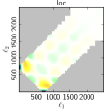
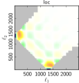
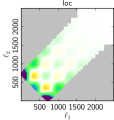
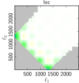
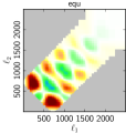
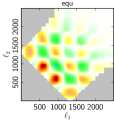
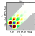
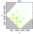
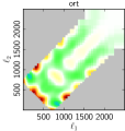
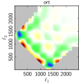
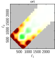
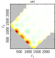
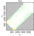
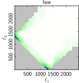
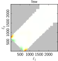
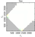
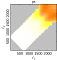
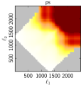
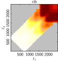
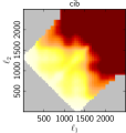
Figure 8: Smoothed theoretical templates for (from top to bottom) the local, equilateral, orthogonal, lensing-ISW, unclustered point sources, and CIB (clustered) point sources shapes, as defined in Section 3.1.1. The templates are normalized by the expected standard deviation of the bispectrum (using the beam and noise characteristics of Section 4), so that a dimensionless signal-to-noise bispectrum results. Moreover, they have all been multiplied by such $f_{\mathrm{NL}}$ values as would give a $30\sigma$ detection. The first two columns are for $TTT$, respectively for $\ell\in$ [700, 741] and $\ell\in$ [1291, 1345], while the two last columns show the same $\ell$ ranges, but for $EEE$. Except for the last line, which contains both point source templates for $TTT$ only.

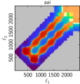
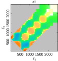
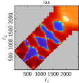
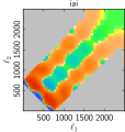
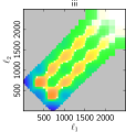
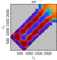
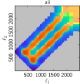
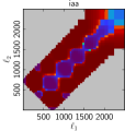
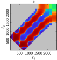
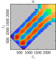
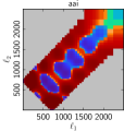
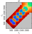
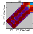
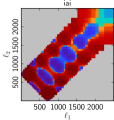
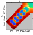
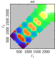
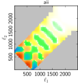
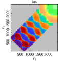
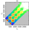
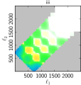
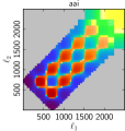
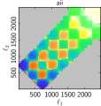
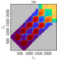
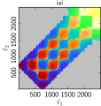
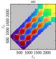
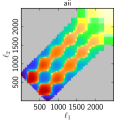
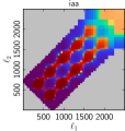
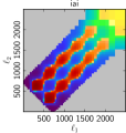
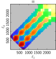
Figure 9: Smoothed theoretical isocurvature bispectra for $\ell_{3}\in$ [700, 741]. The first row presents the 5 different $TTT$ bispectra one can have when considering just the adiabatic and the cold dark matter density isocurvature mode, excluding the purely adiabatic bispectrum. The second and third row are the same, but taking instead the neutrino density and neutrino velocity isocurvature mode, respectively. Finally the last three rows are similar to the first three, but for $EEE$. The bispectra, all with $f_{\mathrm{NL}}=1$, have been normalized by the expected standard deviation assuming the beam and noise characteristics of Section 4, so that a dimensionless signal-to-noise bispectrum results. The colour scale is logarithmic (with the white in the middle corresponding to values smaller than $10^{-9}$ in absolute value).

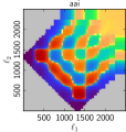
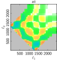
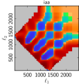
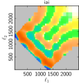
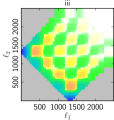
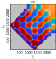
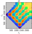
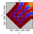
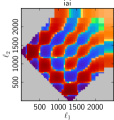
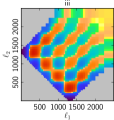
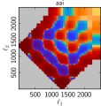
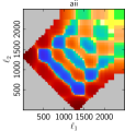
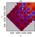
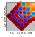
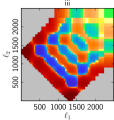
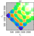
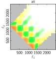
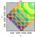
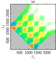
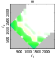
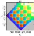
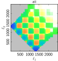
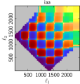
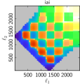
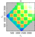
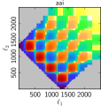
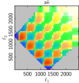
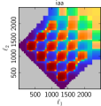
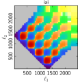
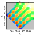
Figure 10: Similar to Fig. 9, but for $\ell_{3}\in$ [1291, 1345].

References

- [1] J. M. Maldacena, Non-Gaussian features of primordial fluctuations in single field inflationary models, JHEP 0305 (2003) 013, [astro-ph/0210603].
- [2] V. Acquaviva, N. Bartolo, S. Matarrese, and A. Riotto, Second order cosmological perturbations from inflation, Nucl.Phys. B667 (2003) 119–148, [astro-ph/0209156].
- [3] M. Liguori, E. Sefusatti, J. R. Fergusson, and E. P. S. Shellard, Primordial Non-Gaussianity and Bispectrum Measurements in the Cosmic Microwave Background and Large-Scale Structure, Advances in Astronomy 2010 (2010) 73, [arXiv:1001.4707].
- [4] Planck Collaboration, Planck 2013 Results. XXIV. Constraints on primordial non-Gaussianity, Astron.Astrophys. 571 (2014) A24, [arXiv:1303.5084].
- [5] Planck Collaboration, Planck 2015 results. XVII. Constraints on primordial non-Gaussianity, arXiv:1502.01592.
- [6] X. Luo, The Angular bispectrum of the cosmic microwave background, Astrophys. J. 427 (1994) L71, [astro-ph/9312004].
- [7] M. Bucher, B. Van Tent, and C. Carvalho, Detecting Bispectral Acoustic Oscillations from Inflation Using a New Flexible Estimator, Mon. Not. Roy. Astron. Soc. 407 (2010) 2193–2206, [arXiv:0911.1642].
- [8] B. Casaponsa, R. B. Barreiro, E. Martinez-Gonzalez, A. Curto, M. Bridges, and M. P. Hobson, Exploring local fNL estimators based on the binned bispectrum, Mon. Not. Roy. Astron. Soc. 434 (2013) 796, [arXiv:1305.0671].
- [9] M. G. Santos et al., Multiple methods for estimating the bispectrum of the Cosmic Microwave Background with application to the MAXIMA data, Mon. Not. Roy. Astron. Soc. 341 (2003) 623, [astro-ph/0211123].
- [10] E. Komatsu, D. Spergel, and B. Wandelt, Measuring primordial non-Gaussianity in the cosmic microwave background, Astrophys.J. 634 (2005) 14–19, [astro-ph/0305189].
- [11] A. Yadav, E. Komatsu, and B. Wandelt, Fast Estimator of Primordial Non-Gaussianity from Temperature and Polarization Anisotropies in the Cosmic Microwave Background, Astrophys.J. 664 (2007) 680–686, [astro-ph/0701921].
- [12] A. Yadav, E. Komatsu, B. Wandelt, M. Liguori, F. Hansen, et al., Fast Estimator of Primordial Non-Gaussianity from Temperature and Polarization Anisotropies in the Cosmic Microwave Background II: Partial Sky Coverage and Inhomogeneous Noise, Astrophys.J. 678 (2008) 578–582, [arXiv:0711.4933].
- [13] J. R. Fergusson, M. Liguori, and E. P. S. Shellard, General CMB and Primordial Bispectrum Estimation I: Mode Expansion, Map-Making and Measures of f_NL, Phys. Rev. D82 (2010) 023502, [arXiv:0912.5516].
- [14] J. R. Fergusson, M. Liguori, and E. P. S. Shellard, The CMB Bispectrum, JCAP 1212 (2012) 032, [arXiv:1006.1642].
- [15] J. R. Fergusson, Efficient optimal non-Gaussian CMB estimators with polarisation, Phys. Rev. D90 (2014), no. 4 043533, [arXiv:1403.7949].
- [16] A. Curto, E. Martinez-Gonzalez, and R. B. Barreiro, On the optimality of the spherical Mexican hat wavelet estimator for the primordial non-Gaussianity, Mon. Not. Roy. Astron. Soc. 412 (2011) 1038, [arXiv:1007.2181].
- [17] X. Lan and D. Marinucci, The needlets bispectrum, Electronic Journal of Statistics 2 (2008) 332–367, [arXiv:0802.4020].
- [18] A. Ducout, F. Bouchet, S. Colombi, D. Pogosyan, and S. Prunet, Non Gaussianity and Minkowski Functionals: forecasts for Planck, Mon. Not. Roy. Astron. Soc. 429 (2013) 2104, [arXiv:1209.1223].
- [19] D. Munshi and A. Heavens, A New Approach to Probing Primordial Non-Gaussianity, Mon. Not. Roy. Astron. Soc. 401 (2010) 2406, [arXiv:0904.4478].
- [20] M. Kamionkowski and T. Souradeep, The Odd-Parity CMB Bispectrum, Phys. Rev. D83 (2011) 027301, [arXiv:1010.4304].
- [21] M. Shiraishi, M. Liguori, and J. Fergusson, General parity-odd CMB bispectrum estimation, JCAP 1405 (2014) 008, [arXiv:1403.4222].
- [22] M. Shiraishi, M. Liguori, and J. R. Fergusson, Observed parity-odd CMB temperature bispectrum, JCAP 1501 (2015), no. 01 007, [arXiv:1409.0265].
- [23] P. Creminelli, A. Nicolis, L. Senatore, M. Tegmark, and M. Zaldarriaga, Limits on non-gaussianities from wmap data, JCAP 0605 (2006) 004, [astro-ph/0509029].
- [24] E. Komatsu and D. Spergel, Acoustic signatures in the primary microwave background bispectrum, Phys.Rev. D63 (2001) 063002, [astro-ph/0005036].
- [25] D. Babich, P. Creminelli, and M. Zaldarriaga, The Shape of non-Gaussianities, JCAP 0408 (2004) 009, [astro-ph/0405356].
- [26] J. Fergusson and E. Shellard, The shape of primordial non-Gaussianity and the CMB bispectrum, Phys.Rev. D80 (2009) 043510, [arXiv:0812.3413].
- [27] E. Tzavara and B. Van Tent, Bispectra from two-field inflation using the long-wavelength formalism, JCAP 1106 (2011) 026, [arXiv:1012.6027].
- [28] N. Bartolo, S. Matarrese, and A. Riotto, On non-Gaussianity in the curvaton scenario, Phys. Rev. D69 (2004) 043503, [hep-ph/0309033].
- [29] L. Senatore, K. Smith, and M. Zaldarriaga, Non-Gaussianities in Single Field Inflation and their Optimal Limits from the WMAP 5-year Data, JCAP 1001 (2010) 028, [arXiv:0905.3746].
- [30] F. Lacasa, A. Penin, and N. Aghanim, Non-Gaussianity of the cosmic infrared background anisotropies – I. Diagrammatic formalism and application to the angular bispectrum, Mon. Not. Roy. Astron. Soc. 439 (2014), no. 1 123–142, [arXiv:1312.1251].
- [31] D. Goldberg and D. Spergel, Microwave background bispectrum. 2. A probe of the low redshift universe, Phys.Rev. D59 (1999) 103002, [astro-ph/9811251].
- [32] K. Smith and M. Zaldarriaga, Algorithms for bispectra: Forecasting, optimal analysis, and simulation, Mon.Not.Roy.Astron.Soc. 417 (2011) 2–19, [astro-ph/0612571].
- [33] A. Lewis, A. Challinor, and D. Hanson, The shape of the CMB lensing bispectrum, JCAP 1103 (2011) 018, [arXiv:1101.2234].
- [34] D. Langlois and B. Van Tent, Hunting for Isocurvature Modes in the CMB non-Gaussianities, Class.Quant.Grav. 28 (2011) 222001, [arXiv:1104.2567].
- [35] D. Langlois and B. Van Tent, Isocurvature modes in the CMB bispectrum, JCAP 1207 (2012) 040, [arXiv:1204.5042].
- [36] M. Bucher and T. Louis, Filling in cosmic microwave background map missing data using constrained Gaussian realizations, Mon. Not. Roy. Astron. Soc. 424 (2012) 1694–1713, [arXiv:1109.0286].
- [37] P. Abrial, Y. Moudden, J. Starck, B. Afeyan, J. Bobin, J. Fadili, and M. Nguyen, Morphological Component Analysis and Inpainting on the Sphere: Application in Physics and Astrophysics, J. Fourier Analysis and Applications 6 (2007) 729.
- [38] P. Abrial, Y. Moudden, J.-L. Starck, J. Fadili, J. Delabrouille, et al., CMB data analysis and sparsity, Statistical Methodology 5 (2008) 289, [arXiv:0804.1295].
- [39] L. Perotto, J. Bobin, S. Plaszczynski, J.-L. Starck, and A. Lavabre, Reconstruction of the CMB lensing for Planck, Astron. & Astroph. 519 (2010) 4, [arXiv:0903.1308].
- [40] K. Smith, L. Senatore, and M. Zaldarriaga, Optimal limits on from WMAP 5-year data, JCAP 0909 (2009) 006, [arXiv:0901.2572].
- [41] F. Elsner and B. Wandelt, Efficient Wiener filtering without preconditioning, Astron. Astrophys. 549 (2013) A111, [arXiv:1210.4931].
- [42] M. Abramowitz and I. Stegun, Handbook of Mathematical Functions. Dover Publications, 1965.
- [43] J. Delabrouille et al., The pre-launch Planck Sky Model: a model of sky emission at submillimetre to centimetre wavelengths, Astron. Astrophys. 553 (2013) A96, [arXiv:1207.3675].
- [44] Planck Collaboration, Planck 2015 results. XII. Full Focal Plane simulations, arXiv:1509.06348.
- [45] K. M. Gorski, E. Hivon, A. J. Banday, B. D. Wandelt, F. K. Hansen, M. Reinecke, and M. Bartelman, HEALPix - A Framework for high resolution discretization, and fast analysis of data distributed on the sphere, Astrophys. J. 622 (2005) 759–771, [astro-ph/0409513].