On the evolution of particle-puffs in turbulence

Abstract

We study the evolution of turbulent puffs by means of high-resolution numerical simulations. Puffs are bunches of passive particles released from an initially spherical distribution at regular time intervals of the order of the Kolmogorov time. The instantaneous shapes of particle puffs, in particular their asphericity and prolateness, are characterized by measuring the gyration tensor. Analysis has been performed by following, up to one large scale eddy-turn-over time, more than $10^{4}$ different puffs, each made of 2000 particle tracers, emitted from different places in a homogeneous and isotropic turbulent fluid with Taylor-scale Reynolds number $Re_{\lambda}\sim 300$. We also analyze the probability of hitting a given target placed downstream with respect to the local wind at the time of emission, presenting data for three different cases: (i) without any reconstruction of the shape, i.e. considering the bunch of point tracers, and approximating the particle-puff as a (ii) sphere or as an (iii) ellipsoid. The results show a strong dependence on the fluctuations of the instantaneous wind at the moment of the emission and appear to be robust with respect to the approximations (i)-(iii).

1 Introduction

Understanding the dispersion and evolution of particles in turbulent flows is a fundamental problem with applications in different fields ranging from atmospheric and oceanic sciences [1, 2, 3, 4, 5, 6] to chemical engineering and astrophysics [7, 8, 9, 10] and even behavioral biology [11]. At high Reynolds numbers, molecular diffusion is negligible and turbulence dominates the transport of momentum, temperature, humidity, salinity and of all other chemical species possibly present in the environment. Turbulent diffusion can be studied from an Eulerian point of view, following the evolution of a concentration field [12, 13] or using a Lagrangian approach in terms of particle tracers advected by the flow [14, 15].

In this paper we discuss an important set-up, namely when particles are emitted as a puff, localized in time and in space. The main aim is to understand the evolution of the shapes of these particle-puffs, quantifying the time evolution of both the growth rate of their typical size and the deviation from a perfect spherical shape. The evolution is followed from the initial instant, when each particle puff is spherical and with size $\sim\eta$, the turbulent Kolmogorov scale, up to the final time of order of one eddy turnover time, when the bunches of particles have reached a typical scale as big as the largest eddy correlation length. We quantify the initial distortion from the spherical shape induced by the intermittent and intense stretching of the local gradients and the shape’s evolution for intermediate times, when the characteristic bunch size is within the inertial range of scales. Because of the many-body nature of our experiments, one expects different informations with respect to those obtained measuring the well known two-particles Richardson dispersion [14, 16, 17], still anticipating however some connections between the two.

As always in passive transport problems [15], there is a one-to-one dictionary that maps Lagrangian concepts into Eulerian ones. Here, the Eulerian counterpart of puff dispersion is the emission of a passive scalar field from a localized source. This problem has many relevant applications, from environmental fluid mechanics, e.g. the dispersal of noxious chemicals in the atmosphere or in the oceans [18], to biology, e.g. long-range olfactory communication through the emission of volatile pheromones [19]. The statistics and dynamics of the concentration field at a distance from the emitting source can thus be put in direct correspondence with puff dispersion. Notably, the alternation of clear-air (blanks) and chemically-loaded pockets (whiffs) that is observed away from the source is connected with the probability that a puff hits a target at a distance from the point where it has been delivered, and among the events where the concentration is detectable, large intensities are due to puffs that disperse poorly (see e.g. [11] for a detailed explanation). Turbulence, therefore, plays a major role in determining the intensity and the temporal structure of the signal, by shaping the information content of the odor message in the case of olfactory communication, or by affecting the probability of reaching lethal doses in environmental applications.

The paper is organized as follows. In Section 2, we introduce and analyze the main quantities which have been used to characterize the puff geometry, namely asphericity and prolateness, which, together with the radius of gyration, summarize the geometrical information contained in the gyration tensor. We show that the most important signature in the two observables is that they approach a peak value, corresponding to maximally elongated puffs, at a time $t\sim 10\tau_{\eta}$. We understand this phenomenology as due to the physics of the dissipative range where the puff, being still of size $\sim\mathcal{O}(\eta)$, is controlled by the stretching rate. Indeed, we show that the initial evolution of these observables can be reasonably estimated considering the bunch stretched with exponential rates given by the three Lyapunov exponents of the underlying fluid. Another remarkable result is obtained for longer times, when we measure a very slow recovery of the isotropic shape, revealing that the typical puff is non spherical, at least, as far as the evolution pertains to spatial and temporal scales in the inertial range. In Section 3, we exploit the link between the Eulerian and Lagrangian language and use the statistics of puffs hitting a given target to estimate the probability of time durations of blanks and whiffs typical of passive scalar fields emitted from a point source. We find that the fluctuations of the instantaneous wind at the instant of the emission are crucial to identify the right downstream direction where to place the target. Moreover, we show that the probability of observing a whiff or a blank lasting for a time $t$ has a power law behavior for small times in fair agreement with the prediction obtained in [11], using dimensional estimate based on exit-time statistics of turbulent diffusion.

2 Evolution of particle-puff geometry due to turbulence

The data analyzed in this paper have been previously obtained in [20] from a direct numerical simulations (DNS) of the Navier-Stokes equations in three dimensions with an isotropic and homogeneous large-scale forcing in a tri-periodic domain. As explained in [20], each puff is composed of $N_{P}$ particles, emitted from a point-like source within the simulation box. Particle bunches are initially distributed uniformly in a sphere of size of order of the Kolmogorov length scale $\eta$, and are emitted one by one every Kolmogorov time, $\tau_{\eta}$, till about one large-scale eddy turnover time, $T_{E}$, for a total of 80 emissions per source. The total integration time of the DNS is of about $2T_{E}$. Table 1 summarizes the main parameters the DNS.

$Re_{\lambda}$	$N^{3}$	$\eta$	$\Delta x$	$\varepsilon$	$\tau_{\eta}$
280	$1024^{3}$	0.005	0.006	0.81	0.033
$T_{E}/\tau_{\eta}$	$u_{rms}$	$N_{P}$	$N_{sou}$	$N_{puff}$	$T_{traj}/\tau_{\eta}$
80	1.7	2000	256	20480	160

Table 1: Main parameters of DNS (all dimensional quantities are expressed in simulations units): $Re_{\lambda}$ Taylor-scale-based Reynolds number, $N^{3}$ grid resolution, $\eta$ and $\tau_{\eta}$ Kolmogorov length and time scales, $\Delta x$ grid spacing, $\varepsilon$ mean energy dissipation, $\nu$ kinematic viscosity, $T_{E}$ large-scale eddy turnover time, $u_{rms}$ root-mean-square velocity, $N_{P}$ number of particle tracers within each puff, $N_{sou}$ number of localized sources within the simulation box, $N_{puff}$ total number of puffs in the simulation domain, $T_{traj}$ maximal duration of particle trajectories. The numerical domain is cubic, with periodic boundary conditions in all directions; a fully dealiased pseudo-spectral algorithm with second order Adams-Bashforth time-stepping has been used. The statistically isotropic and homogeneous external forcing injects energy in the first low-wavenumber shells, by keeping constant in time their spectral content, see [21].

Once emitted, the particle puffs are transported and deformed by the turbulent flow. At least at low-order, we can describe their main geometrical features by measuring the gyration tensor, $\textbf{G}(t)$, with elements

$$G^{ij}(t)=\frac{1}{N_{P}}\sum_{n=1}^{N_{P}}(r^{i}_{n}(t)-r^{i}_{CM}(t))(r^{j}_{n}(t)-r^{j}_{CM}(t)),\ \ \ i,j=x,y,z$$ (1)

where $r^{i}_{n}(t)$ is the $i$-th coordinate of the $n$-th particle of a given bunch after a time $t$ from its emission, and the subscript ${\it CM}$ stands for the center of mass. In particular, the three eigenvalues, $\{g_{i}(t)\}_{i=1}^{3}$, of $\textbf{G}(t)$ bear information about both the size and the shape of the puffs (see, e.g., [22, 23]). For instance, their sum, corresponding to the trace of the gyration tensor, provides the squared radius of gyration $R_{G}^{2}(t)$, namely the bunch characteristic size approximated with a sphere of radius $R_{G}(t)$:

$$\sum_{i=1}^{3}G^{ii}(t)=\sum_{i=1}^{3}g_{i}(t)=R_{G}^{2}(t)\$$ (2)

On the other hand, the three eigenvalues corresponds to the square of the semi-axes of the ellipsoid which best approximates the particle bunch. In Figure 1 we show a schematic picture of the evolution of a given puff, and we explain the link between the bunch shape and both $R_{G}$ and the eigenvalues $g_{i}$.

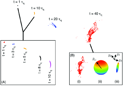
Figure 1: Evolution of a given puff in space, showed at four different instants of time between $t=1\tau_{\eta}$ and $t=40\tau_{\eta}$. (A): the same puff evolution showed between $t=1\tau_{\eta}$ and $t=10\tau_{\eta}$, to illustrate how the puff undergoes a big deformation at small times, passing from a spherical shape to an elongated one. (B): the puff for $t=40\tau_{\eta}$ in the main picture is here represented (i) with the individual particles composing it, (ii) approximated with a sphere of radius $R_{G}$ (the black arrow) or (iii) approximated with an ellipsoid of axes $\sqrt{g_{i}}$, with $i=1,2,3$, and orientation given by the direction of the three eigenvectors of the gyration tensor (the three black arrows). Both the sphere and the ellipsoid are centered in the center of mass of the puff.

A first glimpse into the evolution of puffs can be obtained by looking at the behavior of the three eigenvalues averaged over all sources and emissions, $\langle g_{i}(t)\rangle$, as a function of the time from their emission (Figure 2).

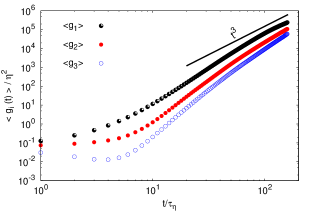
Figure 2: Log-log plot of the evolution of the mean eigenvalues $\langle g_{1}\rangle$, $\langle g_{2}\rangle$ and $\langle g_{3}\rangle$ of the gyration tensor $\textbf{G}(t)$ versus time. The straight line is proportional to $t^{3}$ and corresponds to the Richardson law (3). The three eigenvalues start with very close values (not shown), typical of a spherical bunch, and then separate quickly, to end up with slightly different values, which means that on average the bunch does not return to a spherical shape.

Two regimes are easily detectable. At short times, when the puff size is below or comparable to the Kolmogorov length scale, the dynamics is expected to be controlled by the dissipative range physics and thus by the exponential stretching rates. In other terms, ignoring effects due to stretching rates fluctuations [24, 25], we can approximatively assume that the eigenvalues $g_{i}$ are linked to the Lyapunov exponents $\lambda_{i}$ through the relation $\lambda_{i}\approx\ln\langle g_{i}(t)\rangle/2t$. The factor 2 in the denominator comes from the fact that the gyration tensor is quadratic in particle separations. The Lyapunov exponents characterizing the dynamics of particle tracers in turbulent flows have been measured in several studies [26, 27, 28], here we refer to the values measured in [28]: $\lambda_{1}\sim 0.14/\tau_{\eta}$, $\lambda_{2}\sim 0.04/\tau_{\eta}$, and $\lambda_{3}=-\lambda_{2}-\lambda_{1}$, as $\Sigma_{i}\lambda_{i}=0$, due to fluid incompressibility. In Figure 2 we can see that $\langle g_{1}(t)\rangle$ grows faster than the other two, being associated with $\lambda_{1}$, $\langle g_{2}(t)\rangle$ grows slower, whereas $\langle g_{3}(t)\rangle$ decreases initially due to the fact that $\lambda_{3}$ is negative, indicating that at the early stage of the evolution the spherical bunch tends to preserve the volume while fluid gradients deform it.

At a later time, for $t\gtrsim 10\tau_{\eta}$ all three typical sizes are inside the inertial range, we would then expect the Richardson scaling for all eigenvalues [27, 29]:

$$\langle g_{i}(t)\rangle=g_{R}\epsilon t^{3}$$ (3)

where $g_{R}$ is the universal Richardson constant and $\epsilon$ is the mean energy dissipation of the fluid. As one can see from the figure, this scaling behavior is barely achieved only for large times in agreement also with the behavior of the eigenvalues of the inertia tensor for particle tetrads [27]. This deviation from Richardson can be explained as due to the contamination induced by the fluctuations of the viscous scale leading to the presence of bunches of various sizes (even of order $\eta$) also at long times after the emission, see [20, 30] for a detailed study of this effects on the same data set. It is interesting to remark, that the three curves tend to proceed parallel when inside the inertial range. They show a tendency to converge to the same value only at very long times when the dynamics is essentially diffusive, as above the largest scale of turbulence velocity correlations are washed out. This means that in the inertial range the single puff, either never recovers isotropy (i.e. a spherical shape) or it does it very slowly. This is an important observation as it tells us that it would be wrong to describe a typical puff evolving in a turbulent flow in terms of a spherical shape, even if the underlying turbulence is isotropic.

In the remainder of this section we quantify these deviations from spherical symmetry. To this aim we adopt two well known quantities [31, 32] defined in terms of the eigenvalues of $\textbf{G}(t)$, the asphericity and prolateness. The asphericity is given by the normalized variance of the three eigenvalues,

$$A(t)=\frac{1}{6}\sum_{i=1}^{3}\frac{(g_{i}(t)-\overline{g(t)})^{2}}{\overline{g(t)}^{2}}$$ (4)

where $\overline{g(t)}=\sum_{i=1}^{3}g_{i}(t)/3$. Clearly, we have that $A$ ranges from $0$, when all eigenvalues are equal and the bunch is spherical, to 1 with only one eigenvalue different from zero, meaning a totally aspherical bunch. The prolateness:

$$P(t)=\frac{\prod_{i=1}^{3}(g_{i}(t)-\overline{g(t)})}{\overline{g(t)}^{3}}\$$ (5)

is defined in the interval $[-1/4,2]$ and tells us whether the shape of the bunch is oblate or prolate. In particular, $P(t)>0$ means $g_{1}\gg g_{2}\approx g_{3}$, i.e. the bunch has a prolate shape becoming a rod in the limit $P=2$, while $P(t)<0$ means $g_{1}\approx g_{2}\gg g_{3}$ that is the bunch is oblate, tending to a disk for $P=-1/4$.

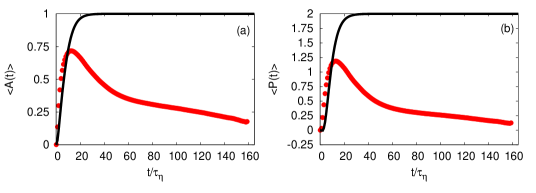
Figure 3: (a): Lin-Lin plot of the mean asphericity $\langle A(t)\rangle$ versus time (points). The value at time $t=0$ is very small $\approx 10^{-3}$, because the bunch is injected with a spherical shape. At the end of its evolution $\langle A(t)\rangle$ does not return close to zero, that is the bunch does not recover a spherical shape. The solid black line approximating the initial growth is evaluated assuming the Lyapunov dynamics for the eigenvalues, i.e. replacing $g_{i}(t)$ with $e^{2\lambda_{i}t}$ (see text for the Lyapunov values). The peak in the real evolution of the asphericity corresponds to $t/\tau_{\eta}\approx 13$, i.e. the time when the size of the puffs starts to be dominated by non-linear effects. (b): the same discussion for the asphericity applies to the prolateness.

In Figure 3a-b we show the evolution of the asphericity and prolateness, averaged over all emissions, $\langle A(t)\rangle$ and $\langle P(t)\rangle$, respectively. As at the emission time $t=0$ each particle bunch is injected uniformly within a sphere of radius $\sim\mathcal{O}(\eta)$, the initial values are close to zero $\langle A(0)\rangle\sim\mathcal{O}(10^{-3})$ and $\langle P(0)\rangle\sim\mathcal{O}(10^{-6})$.

At initial times, while the bunch size is within the dissipation range (for $t\lesssim 10\tau_{\eta}$), the asphericity grows very rapidly, reaching a peak value $\approx 0.7$ at $t\approx 13\tau_{\eta}$. This means that the dissipative scale stretching mechanism is very efficient in transforming the sphere in a prolate ellipsoid, as confirmed by the average prolateness (Fig. 3b) which reaches a peak value $\approx 1.2$ when $\langle A(t)\rangle$ is maximal. This kind of evolution is indeed expected due to the presence of two positive Lyapunov exponents [26, 27, 28]. As shown in Figure 3, the initial growth of both asphericity and prolateness is well captured by their approximations obtained from (4) and (5) by replacing $g_{i}(t)$ with $e^{2\lambda_{i}t}$. We notice that the actual data grow slightly faster than that predicted by the Lyapunov exponent approximation, this discrepancy might be due to the fact that we neglected fluctuations of the stretching rates [24, 25]. Notice that at time long enough the (linear) approximation reaches the asymptotic values typical of a rod like structure, as the approximation does not include neither folding mechanism nor the physics of the inertial range with the Richardson diffusion.

After the peak, both the asphericity and the prolateness show a slow decay toward lower values, but even for times larger than the large-scale eddy turnover time, the shape of the bunch does not return spherical. Clearly, at very long times, where only diffusion is taking place, we expect to recover a spherically symmetric puff, but this does not seem to be the case within the inertial range.

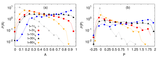
Figure 4: Probability density functions for the asphericity (a) and the prolateness (b), at various times, $t=1\tau_{\eta}(\Diamond)$, $t=3\tau_{\eta}(\square)$, $t=10\tau_{\eta}(\bigcirc)$, $t=30\tau_{\eta}(\bigtriangleup)$, $t=80\tau_{\eta}(\bigtriangledown)$. Even at large times there is still a considerable number of puffs far from having a spherical shape.

In Figure 4a-b we show the probability density functions (PDFs) for the asphericity and the prolateness, respectively, at various times. After a time interval of approximately $t\sim 10\tau_{\eta}$, that corresponds to the peak values of Figure 3a-b, we observe that turbulent stretching has produced bunches with all possible values of $A$ and $P$ with a higher probability for very elongated ellipsoid. For later times, a slow return toward the spherical values is observed, with the development of a peak at $A=P=0$. Notice however that, even for very large times, both PDFs show the presence of a large sub-set of bunches that are far from being spherical, a clear and important legacy of small-scale turbulent fluctuations for the whole time history of every bunch.

3 Blanks and whiffs

In view of the presence of a non negligible set of bunches with a non-spherical shape one might want to assess the effects of shape distribution on the probability of hitting a target and how this impacts the concentration statistics in a given point downstream of the emitting source. In particular, we are interested to compare three different cases: (i) considering the puff as formed by individual particles, (ii) approximating it as a sphere with a radius given by its mean radius of gyration or (iii) approximating it as an ellipsoid with the three main axes given at any time by the value of the three eigenvalues $g_{i}(t)$. Of course the probability to hit the target will strongly depend on the presence (or absence) of a mean wind, on the distance between the source and the target and on the wiggling motion of the center of mass of the puff induced by turbulent fluctuations. In the present case, because of the absence of a steady mean wind, we have always conditioned the position downstream of the target to be aligned with the direction of the velocity in the position of the source at the instant of the emission. We also adopted a definition of (local) mean wind based on the average displacement of the center of mass of all puffs emitted by the same source. We found that the results do not depend too strongly on the adopted definition provided the target is at distance lower than the large scale of the flow. Indeed the local wind being a large scale quantity will persist on the time scale of the largest length scale. In absence of this fine tuning, the probability to hit the target decreases to values that are not statistically significant (not shown). For sake of definiteness, the target has always been taken spherical, of radius $R=4\eta$ and placed at distance $D=40\eta$ from the source, along the direction given by the (local) mean wind.

Figure 5: Histogram of the signal of the concentration of particles for a single source. The target is placed at a distance $D=40\eta$ from the source, along the direction given by the mean wind, and all the values of concentration are divided by the total number of particles that compose a puff. Periods of presence of signal (whiffs) and of absence of signal (blanks) can be distinguished.

Notwithstanding the huge data set, the lack of a stable mean wind makes this kind of measurement very delicate, as the puff is advected by the mean velocity of its center of mass, which is a highly fluctuating quantity if the puff has a relatively small size. As a result only rarely the bunches hit the target and the signal given by the superposition of the puff with the target is very intermittent. The only stable probability we could measure is the time elapsed between two consecutive hits (the time span of a blank $t_{b}$), and the time duration of a detection (the time span of a whiff $t_{w}$), independently of the amount of particles detected. Both times are predicted to have a power law distribution at least for short durations, when the determination of a blank or a whiff is due to the three-dimensional diffusive motion of the center of mass of the bunch around the target [11]:

$$P(t_{b})\sim t_{b}^{-3/2};\qquad P(t_{w})\sim t_{w}^{-3/2}$$ (6)

According to this picture, the beginning of a whiff occurs when the puff is barely within the target, i.e. the center of the bunch is at a distance of order $R_{G}$ from the target. The end of the whiff will occur when the puff first exits from the target. Therefore, the duration is distributed as the first exit time for a diffusion process, whence the power law $3/2$ in (6). For events of a longer duration an exponential tail should emerge (see [11] for a detailed modelization at all times). Similarly, the duration $t_{b}$ of blanks is the time needed for a diffusing puff that has lost contact from the target to regain contact with it. It follows from arguments symmetric to those discussed for the whiffs that blank intervals are distributed as $t^{-3/2}$ as well.

The signal of the concentration of particles within the target for a specific source is presented in Figure 5. The heights of the histogram represent the values of concentration divided by the total number of particles in a bunch. These are evaluated integrating over all the time the bunch remains within the target. The signal is intermittent and very similar to those obtained experimentally, and we can distinguish periods of absence of signal (blanks) and periods of presence of signal (whiffs). Blanks correspond to the case in which the bunch does not intersect the target and passes by. On the contrary whiffs correspond to the case in which the bunch is partially or entirely inside the target. As from equation (2) we can consider the bunch not only as a discrete object composed of particles, but also as a sphere of radius $R_{G}$ or as an ellipsoid with semi-axes given by $\sqrt{g_{1}}$, $\sqrt{g_{2}}$ and $\sqrt{g_{3}}$. In all these three cases, we can reconstruct the probability density functions of blanks and whiffs.

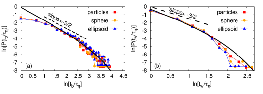
Figure 6: PDF of the duration $t_{b}$ of blanks (a), i.e. time intervals without signal, and PDF of the duration $t_{w}$ of whiffs (b), i.e. time intervals with signal, for the bunch considered as composed of particles ($\square$) and approximated with a sphere ($\bigcirc$) and an ellipsoid ($\bigtriangleup$). On the axes, the natural logarithms of $t_{b}$ $(t_{w})$ and $P(t_{b})$ $(P(t_{w}))$ are reported. The dashed line has slope equal to -3/2 and represents the expected trend for small times, $P(t_{b})\sim t_{b}^{-3/2}$ for blanks and $P(t_{w})\sim t_{w}^{-3/2}$ for whiffs, while the solid line represents the expected trend for the entire PDF, $P(t_{b})\sim t_{b}^{-3/2}e^{-t_{b}/T}$ for blanks and $P(t_{w})\sim t_{w}^{-3/2}e^{-t_{w}/T}$ for whiffs. The PDFs are obtained considering a threshold value for concentration, i.e. not considering in the signals, as for instance the one shown in Figure 5, heights smaller than $10^{-2}$.

The PDF of the blanks is shown in Figure 6a, for the bunch taken as discrete and approximated with a sphere and an ellipsoid. The dashed black line represents the law we expect the three cases will follow for small $t_{b}$s, i.e. (6), while the solid black line is the expected trend for the entire PDF, i.e. equation (6) times an exponential term $\sim e^{-t_{b}/T}$. Very short blanks tend to be less frequent, as it is unlikely that a puff crosses the target, leaves it and then hits back after a time of order $\tau_{\eta}$. The PDF of the whiffs is instead shown in Figure 6b. Since blanks and whiffs are complementary, we expect the same law. In this case we expect instead few whiffs of long duration. Even without a well defined mean wind we could have obtained satisfying results, which suggest blanks and whiffs are two robust observables. As far as our statistics is concerned, using the real discrete shape, the spherical or ellipsoidal approximation has no consequences regarding the probability distribution functions. If this remains the case also with a larger statistics and/or in presence of a mean stable wind is an interesting and open question that we cannot answer within the present data set. However, the argument used in [11] (and briefly discussed above) to derive (6) is rather general depending on the diffusive motion of the center of mass and thus the behavior (6) is not expected to depend too strongly on the representation of the puff.

4 Conclusions

We have studied the evolution of shape of more than $10^{4}$ different puffs transported by a turbulent flow, by means of asphericity and prolateness, following the puffs up to one large-scale eddy turnover time. The puff is emitted spherical in the flow, and we have found a strong distortion of the shape at small times, that is also in agreement with assuming the Lyapunov dynamics for the characteristic dimensions of the puff. Moreover, we have found that notwithstanding the isotropic nature of turbulence, puffs do not fully recover a spherical shape at longer times for a threefold reason: (i) small-scale stretching quickly and strongly distorts the puff (ii) the recovery of isotropy in the inertial range is slow (algebraic) [33] (iii) the inertial range has a limited extent. As a result, the memory of the Lagrangian dynamics in the dissipative range is kept for long times. We have also analyzed the probability of hitting a given target placed downstream with respect to the local wind at the time of emission, in the three cases of the puff considered as a discrete bunch of particles, as a sphere, and as an ellipsoid. We have found a good agreement with the predictions for the probability densities of time periods with and without hits. These results point to the conclusion that the concentration statistics is only mildly affected by the asphericity of the puffs. Our analysis, possibly extended to include the effect of mean wind and shear, may provide valuable suggestions to improve Lagrangian models of puff release in the environment [34, 35, 36].

References

References

- Csanady [1973] G.T. Csanady, Turbulent diffusion in the environment, Ed. D. Reidel Publishing Company, 1973.
- Bennett [1984] A. F. Bennett, Relative dispersion: local and nonlocal dynamics, J. Atmos. Sci., 41 (1984) 1881-1886.
- Lacorata et al. [2008] G. Lacorata, A. Mazzino, U. Rizza, 3D chaotic model for subgrid turbulent dispersion in large eddy simulations, J. Atmos. Sci., 65 (2008) 2389-2401.
- Ollitraut et al. [2005] M. Ollitraut, C. Gabillet, A.C. De Verdiére, Open ocean regimes of relative dispersion, J. Fluid Mech., 533 (2005) 381-407.
- Poulain & Zambianchi [2007] P.M. Poulain, E. Zambianchi, Surface circulation in the central Mediterranean Sea as deduced from Lagrangian drifters in the 1990s, Cont. Shelf Res., 27 (2007) 981-1001.
- LaCasce [2010] J.H. LaCasce, Relative displacement probability distribution functions from balloons and drifters, J. Mar. Res., 68 (2010) 433-457.
- Baldyga & Bourne [1999] J. Baldyga, J.R. Bourne, Turbulent mixing and chemical reactions, Wiley, 1999.
- Hill [1976] J. C. Hill, Homogeneous turbulent mixing with chemical reaction, Annu. Rev. Fluid Mech., 8 (1976) 135-161.
- Lepreti et al. [2012] F. Lepreti, V. Carbone, V.I. Abramenko, V. Yurchyshyn, P.R. Goode, V. Capparelli, A. Vecchio, Turbulent pair dispersion photospheric bright points, Astrophys. J. Lett., 759 (2012) L17.
- Elmegreen [2010] B.G. Elmegreen, A. Burkert, Accretion-driven turbulence and the transition to global instability in young galaxy disks, Astrophys. J., 712 (2010) 294-302.
- Celani et al. [2014] A. Celani, E. Villermaux, M. Vergassola, Odor landscapes in turbulent environments, Phys. Rev. X, 4 (2014) 041015
- Dimotakis [2005] P.E. Dimotakis, Turbulent mixing, Annu. Rev. Fluid Mech., 37 (2005) 329-356.
- Warhaft [2000] Z. Warhaft, Passive scalars in turbulent flows, Annu. Rev. Fluid Mech., 32 (2000) 203-240.
- Sawford [2001] B. Sawford, Turbulent relative dispersion, Annu. Rev. Fluid Mech., 33 (2001) 289-317.
- Falkovich et al. [2001] G. Falkovich, K. Gawȩdzki, M. Vergassola, Particles and fields in fluid turbulence, Rev. Mod. Phys., 73 (2001) 913-975.
- Richardson [1926] L.F. Richardson, Atmospheric diffusion shown on a distance-neighbour graph, Proc. R. Soc. London, Ser A, 110 (1926) 709-737.
- Salazar & Collins [2009] J.P.L.C. Salazar, L.R. Collins, Two-particle dispersion in isotropic turbulent flows, Annu. Rev. Fluid Mech., 41 (2009) 405-432.
- Devaull et al. [1995] G.E. Devaull, J.A. King, R.J. Lantzy, D.J. Fontaine, Understanding atmospheric dispersion of accidental releases, Wiley-AIChE, 1995.
- Wyatt [2003] T.D. Wyatt, Pheromones and animal behavior, Cambridge University Press, 2003.
- Biferale et al. [2014] L. Biferale, A. Lanotte, R. Scatamacchia, F. Toschi, Intermittency in the relative separations of tracers and of heavy particles in turbulent flows, J. Fluid Mech., 757 (2014) 550-572.
- Chen et al. [1993] S. Chen, G.D. Doolen, R.H. Kraichnan, Z.S. She, On statistical correlations between velocity increments and locally averaged dissipation in homogeneous turbulence, Phys. Fluids A, 5 (1993) 458-463.
- Chertkov et al. [1999] M. Chertkov, A. Pumir, B.I. Shraiman, Lagrangian tetrad dynamics and the phenomenology of turbulence, Phys. Fluids, 11 (1999) 2394-2410.
- Toschi & Bodenschatz [2009] F. Toschi, E. Bodenschatz, Lagrangian properties of particles in turbulence, Annu. Rev. Fluid Mech., 41 (2009) 375-404.
- Fujisaka [1983] H. Fujisaka, Statistical dynamics generated by fluctuations of local Lyapunov exponents, Prog. Theor. Phys. 70 (1983) 1264-1275.
- Benzi et al. [1985] R. Benzi, G. Paladin, G. Parisi, A. Vulpiani, Characterisation of intermittency in chaotic systems, J. Phys. A: Math. Gen., 18 (1985) 2157-2165.
- Girimaji & Pope [1990] S.S. Girimaji, S.B. Pope, Material-element deformation in isotropic turbulence, J. Fluid Mech., 220 (1990) 427-458.
- Biferale et al. [2005b] L. Biferale, G. Boffetta, A. Celani, B.J. Devenish, A. Lanotte, F. Toschi, Multi-particle dispersion in fully developed turbulence, Phys. Fluids, 17 (2005) 111701.
- Bec et al. [2006b] J. Bec, L. Biferale, G. Boffetta, M. Cencini, S. Musacchio, F. Toschi, Lyapunov exponents of heavy particles in turbulence, Phys. Fluids, 18 (2006) 091702.
- Pumir et al [2000] A. Pumir, B.I. Shraiman, M. Chertkov, Geometry of Lagrangian dispersion in turbulence, Phys. Rev. Lett., 85 (2000) 5324-5327.
- Scatamacchia et al. [2012] R. Scatamacchia, L. Biferale, F. Toschi, Extreme events in the dispersions of two neighboring particles under the influence of fluid turbulence, Phys. Rev. Lett., 109 (2012) 144501.
- Aronovitz et al. [1986] J.A. Aronovitz, D.R. Nelson, Universal features of polymer shapes, J. Phys., 47 (1986) 1445-1456.
- Blavatska et al. [2010] V. Blavatska, W. Janke, Shape anisotropy of polymers in disordered environment, J. Chem. Phys., 133 (2010) 184903.
- Biferale & Procaccia [2005] L. Biferale, I. Procaccia, Anisotropy in turbulent flows and in turbulent transport, Phys. Rep., 414 (2005) 43-164.
- Haan et al. [1995] P. de Haan, M.W. Rotach, A puff-particle dispersion model, Int. J. Environment and Pollution, 5 (1995) 350-359.
- Haan et al. [1998] P. de Haan, M.W. Rotach, A novel approach to atmospheric dispersion modelling: The Puff-Particle Model, Q. J. R. Meteorol. Soc., 124 (1998) 2771-2792.
- Reynolds [2000] A.M. Reynolds, On the application of a Lagrangian Particle-Puff Model to elevated sources in surface layers with neutral stability, J. Applied Meteorol., 39 (2000) 1218-1228.