The role of the Havriliak-Negami relaxation in the description of local structure of Kohlrausch’s function in the frequency domain. Part I

Abstract

An improved approximation via Havriliak-Negami (HN) functions to the Fourier Transform (FT) of certain Weibull distributions, $-\psi_{\beta}$, (the time derivative of the Kohlrausch-Williams-Watts function), is given for a large interval of frequencies: $\omega/2\pi\in[0,10^{12}]$ if $0<\beta\leq 1$ and $\omega/2\pi\in[0,10^{7}]$ if $1<\beta\leq 2$. The model is free from the usual numerical distortions, or restrictions associated to sampling step and finite size, present in similar adjustments to complex relaxation functions. Further indicates that the identification of (FT) Weibull data with a double HN approximant, $\psi_{\beta}\simeq\mathcal{A}p_{2}HN$, is quite exact locally even though the parameters involved should vary adiabatically with the frequency, i.e. $\{\alpha_{1,2},\gamma_{1,2},\tau_{1,2},\lambda\}(\omega)$. This fact is the base for the high sensibility of the parameter models, as functions of $\beta$, to the available data and sampling associated errors. Presumably is also the root of the different proposals for asymptotic traits of $\alpha\cdot\gamma(\beta)_{1,2}|_{\omega\rightarrow\infty}$ functions found in scientific literature.

¹Instituto de Física Fundamental, IFF-CSIC, Serrano 123, Madrid ES-28006, Spain

²Departamento de Química, Facultad de Ciencias del Mar, ULPGC, Campus Universitario de Tafira, Las Palmas de G. Canaria ES-35017, Spain

Introduction

The Kohlrausch relaxation function, $\phi_{K,\beta}(t)\equiv\exp-t^{\beta}$, $0\leq t<\infty$, $\beta\leq 1$, initially proposed to explain the discharge of capacitors [1], has found later several applications in many fields not directly related to electrostatics. And while it was half-forgotten in the scientific literature which was more worried about practical applications, it did not dissapear at any time of the mathematical heritage due to the deep connections that such function and its sequel, $\beta>1$, have with number theory [2, 3, 4, 5, 6, 7], stable distributions in probability [8, 9, 10, 11, 12, 13, 14], theta function extensions [15, 16], or the special functions obtained from certain kernels of Mellin-Barnes type transformations employed in fractional calculus [17, 18, 19, 20, 21, 22, 23]. However it is a result of its use by Williams and Watts [24], in the field of characterization of dielectric properties of polymers [24, 25, 26], that its employment became ubiquitous in many areas of Physics and Chemistry. Hereafter not only associated with specific electrical phenomena but a plethora of them in the most diverse fields. It emerges in luminiscence [27, 28, 29, 30, 31, 32, 33], supercooled glasses [34, 35, 36], capacitors [1, 37, 38, 39], rheology [40, 41, 42], spin glasses [34], torsion of galvanometric threads [43], dielectric spectroscopy [28, 39, 44, 45, 46, 47, 48, 49], magnetic resonance [50, 51, 52], autocorrelation functions in molecular dynamics [27, 29, 50, 53], econophysics [54, 55], protein folding [20, 33, 56, 57, 58] and even astrophysics [59].

Since it shows up in many branches of physics of complex systems [38, 58, 60, 61, 62] and soft matter [34, 40, 45, 48, 63, 64, 65], among others, seems not be linked to a precise interaction or a particular physico-chemical phenomenon, instead it is more appropriate to associate it to an emergent property. In such a case any ensemble of interacting elements organized in multiscale clusters whose local relaxations, or restructuring bonds, proceed to jumps with random wait times of type $t^{-a}$ should present an autocorrelation, or decay, of Kohlrausch’s nature [35, 40, 42, 62, 66, 67, 68, 69]. Thus its hierarchical structure, and possibly experimental difficulties, advises us to study this relaxation not only through its response along time but also in other spaces of representation, such as of frequency [37, 49, 53, 65, 70, 71, 72, 73, 74]. An exhaustive account of the distribution of intermolecular configurational energies, characteristic relaxation times –real or virtual–, and frequency response will give us a valuable set of techniques to tie in different analytical and laboratory procedures. And indeed such possibilities are available since the Transforms of Fourier and Laplace, ($\omega-$space and $\tau-$space respectively), exist for the case $0<\beta\leq 2$ [8, 9, 10, 12, 13]. Either as a convergent series or an asymptotic one, according to subcases $0<\beta\leq 1$ and $1<\beta\leq 2$ and depending on we are talking about high or low frequency [8, 9, 10, 12, 13, 75].

Unfortunately these series present several problems of convergence mainly near zero, and in particular the best known of them shows up an essential singularity and the others are simply asymptotic [10, 12, 13, 25, 26, 75], i. e. non convergent as a whole, and with coefficients associated to the special function gamma, $\Gamma$, over the entire reals which makes calculations more tedious than in other simpler expressions [44, 50, 76, 77]. This makes the sum of such series a burdensome task which is possible to get round with numerical methods or resummation of series [51, 75, 78, 79]. Nowadays both techniques allow a direct and quick calculation of Laplace and Fourier Transforms with enough accuracy to be of great utility in spectral filtering, or analysis, of laboratory data [75, 78]. Nevertheless could be missed a concise mathematical formula to give account, even approximately, of the mentioned transforms to accelerate the calculations or evaluate repeatedly such functions [53, 65, 70]. The latter is usually a must in optimization since the multiple evaluation of objective functions with variational parameters increases drastically computational loads. Genetic algorithms are a good example of this problem. On the other hand a short analytical expression makes it easier to compare with the most common mathematical functions in the complex domain which are already used in the field of dielectric relaxation, such as Debye [80], Cole-Cole [81], Cole-Davidson [82], Havriliak-Negami [83, 84] and others.

We use the notation $\chi_{\beta}(\omega)=$ $\int_{0}^{\infty}e^{-i\omega t}\phi_{K,\beta}(t)\mathrm{d}t$ for the one-sided Fourier transform of the Kohlrausch function and $\psi_{\beta}(\omega)=$ $-\int_{0}^{\infty}e^{-i\omega t}\frac{d}{dt}\phi_{K,\beta}(t)\mathrm{d}t$ for minus the transformation of the Weibull distribution. They are both related in $\omega-$space by the algebraic closure relationship $\psi_{\beta}(\omega)+i\omega\chi_{\beta}(\omega)$ $=1$. In this way it is indistinct to work with $\psi_{\beta}$ or $\chi_{\beta}$, the former is however preferable since it allows to remove a pole and obliterates any singularity in the neighborhood of $\omega\approx 0$ while using the resummation formula for the original series of inverse powers of $\omega^{\beta}$ which describes $\chi_{\beta}$, (for more details see Ref. [51]). Other advantages of employing $\psi_{\beta}$ are homogeneity, boundedness and similarity of this family of functions if the shape parameter $\beta$ is varied, as we pointed out previously [53]. We will improve this reference, and others similar in nature [37, 49, 70, 71], extending the limits imposed by numerical samplings in $t-$space and making consistent the description of high frequencies decays for $\psi_{\beta}$ with a unique set of strict Havriliak-Negami functions when $\beta\leq 1$, and with set of same kind although parametrically extended if $\beta>1$ [53]. Besides we will show how the apparently supernumerary parameters of the Havriliak-Negami function [83, 84], $\frac{1}{(1+(i\omega\tau_{HN})^{\text{$\alpha$}})^{\gamma}}$, $0<\alpha,\gamma\leq 1$, when approximating the mentioned transform are uniquely determined by the parameter $\beta$. Thus these models with such strong dependency $\{\alpha,\gamma,\text{$\tau$}\}(\beta)$ are equated with others quite new of less parameters [65].

1 Analytical considerations

1.1 The asymptotes of the data

As it was shown [53], a double approximant of Havriliak-Negami functions describe fairly well the FFT of the derivative of the Kohlrausch function as well as the Cole-Davidson-Kohlrausch family [53, 65]. Being the main source of error an small impairment of the fit in the low frequencies. Nevertheless as the FFT is obtained from the original function by means of a finite window sampling, which in the Fourier space is reflected as a convolution with a sinc function, a round off of the spectra in the high frequency border of the domain is obtained. Consequently the asymptotic behaviour of the original function and the approximant will differ, at least in the high frequency domain limits. Besides, due to the smearing of the peaks when the numerical transformation is involved, a difference between the theoretical FT and that of the numerically sampled function is expected. This is why the double approximant fitted to the numerical transformation possibly increments even more than its mathematical limitations the difference with the FT of $\beta t^{\beta-1}e^{-t^{\beta}}$ at the low frequencies. The question raised is then how sensitive are the parameters obtained in the optimization to this deformation, inasmuch as the asymptotic behaviour of the Kohlrausch’s (or Weibull’s [85, 86]) Fourier Transform has been indexed to them (v.gr. $\alpha_{i}\cdot\gamma_{i}=\alpha_{i}\cdot\gamma_{i}(\beta)$ and the rest are functions of $\beta$ too) [70, 71, 87].

To assess the influence of finite-size deformation in the parameters obtained by fitting a couple of Havriliak-Negami functions to the Fourier Transform, $\psi_{\beta}(\omega)$, we have performed two different simulations of it with a general purpose mathematics package (Mathematica^TM). The aim is to obtain accuracy and avoid numerical oscillations as far as possible, the latter a characteristic of the integrals involved that makes difficult results at very high frequencies, as well as to get the proper asymptotic behaviour of the tails.

As it was for the FFT case the first series comprehends frequencies from $\nu=0$ to $\nu$ = 500.0005 in steps of $\delta\nu$ = 1/999.999, being $\omega=2\pi\nu$ [53]. The range of parameter $\beta$ simulated is (0, 2.00], and two subintervals of different traits are analyzed independently. One $\beta\in$(0,1.00] the other $\beta\in$(1.00,2.00] with test points chosen as {0,1}.xy with x = {0,1,2,3,4,5,6,7,8,9} and y = {0,2,5,8} and the end point $\beta$ = 2.00.

For the second series the $\beta$ points are the same aforementioned but the choice for the interval of frequencies is different for each of the cases $\beta\leq$1 and $\beta>$1. So if $\beta\leq$1, $\nu\in$[0,10¹²] and for $\beta>$1, $\nu\in$[0,10⁷] and the reason for these distinct intervals is the increasing numerical noise that overshadows the signal. This makes any calculation useless beyond $\nu$ = 10⁷ for $\beta>$1 and mostly for $\beta\gtrsim$1.90. Besides the steps of frequencies are not homogeneous in the whole interval as they were in the first series; they are now in this way only in logarithmic scale. This is, in the interval $\nu\in$[0,10^-5] the step takes the value $\delta\nu$ = 10^-8, and in each interval $\nu\in$($10^{a_{i}},10^{a_{i}+1}$] the increment is $\delta\nu_{i}=9*10^{a_{i}-3}$ with $a_{i}$ any integer of set {-5,-4,…,-1,0,1,…,11,12} if $\beta\leq$1, or set {-5,-4,…,-1,0,1,…,6,7} if $\beta>$1. So with this second series it is possible to sample a wider domain not affordable with the fine grain step we used in the first series, the drawback here is the different implicit ’weight’ the points acquired in both series when the fitting to a double Havriliak-Negami approximant is made.

The reason for such a large domain of frequencies it is not the reconstruction purpose, as was shown that a domain of low to medium frequencies, (i.e. $\nu\in$[0,500.0005]), were enough to depict the function $e^{-t^{\beta}}$ quite accurately by means of inverse FFT of $\chi_{\beta}(\omega)$ [53]. Nor, of course, the physical reconnaissance by means of dielectric spectroscopy as usually is done in polymer or metallurgical sciences because just one type of relaxation is rarely presented in isolation. Usually different kind of relaxations, associated to several size scales and diverse phenomena, are registered together in contiguous domains of frequency spoiling each diagram the head and tail of its neighbors. Rather we are interested in tails from a mathematical point of view, since a proper knowledge of the function –and this includes the exact tail shape–, will allow us to concoct the more precise approximant possible in the whole domain, and which should include the difficult-by-series description at low frequencies, i.e. near $\nu\sim 0$.

The modulus of function $\psi_{\beta}(\omega)$ presents the following asymptotic behaviour in the domain of frequencies: $|\psi_{\beta}(\omega)|$$\sim$1 when $\omega\rightarrow 0$ and $|\psi_{\beta}(\omega)|$$\sim$$\Gamma(\beta+1)/\omega^{\beta}$ as $\omega\rightarrow\infty$ being monotonically decreasing in the intermediate values. Nevertheless the interval of frequencies in which a significant amount of this dropping takes place depends strongly with the value of parameter $\beta$. While for values near to zero, $\beta\rightarrow 0$, the decrement of the signal is slow and mild, near to one, $\beta\sim 1$, is quicker and sharper. For example in the interval $\nu\in[0.001,500.0005]$, the initial values of $|\psi_{\beta}(\omega)|$ are: (0.665237, 0.793929, 0.999607, 0.999973, 0.999980) and the respective percentage drops are (14.462%, 56.382%, 98.429%, 99.931%, 99.968%), at the end of such domain, when $\beta$ is set to (0.02, 0.10, 0.50, 0.90, 1.00). This suggests important features about the functions $|\psi_{\beta}(\omega)|$, namely the plateau near $\nu\sim 0$ is growing in length as $\beta\rightarrow 1$, the mentioned evolution towards a steeper function, and consequently the less important contribution of the tails to the decrement as $\beta$ varies. Such behaviour is held and even exacerbated in the interval $1<\beta\leq 2$, not only because the drop is greater –(99.9851%, 99.9992%, 99.9999%) for $\beta\in${1.10, 1.50, 2.00}, with starting values (0.999985, 0.999992, 0.999996) of $|\psi_{\beta}(\omega)|$– but also a sudden change in the decreasing of the functions is perceived.

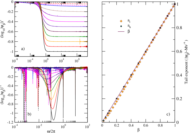
Figure 1: a) Logarithmic derivative of $\log_{10}|\psi_{\beta}(\omega)|$ vs. $\log_{10}(\omega/2\pi)$. b) Logarithmic second derivative of $\log_{10}|\psi_{\beta}(\omega)|$ vs. $\log_{10}(\omega/2\pi)$. c) Exponent $a$ of fitting $|\psi_{\beta}(\omega)|\sim\omega^{-a}$ to data tail. Subindex $l$ refers to a sampling of low to medium frequencies and subindex $h$ to a high frequencies one. Solid line would imply $a\equiv\beta$. See details in text. $\beta\leq 1$.

In order to avoid that these characteristics of the $|\psi_{\beta}|$ functions could make seem them belonging to a irregular family of functions ruled by a parameter, we shall change the scale of the abscissae axis and we will draw our attention to the first and second derivatives of such functions in the new scale. The choice for the axis is the decimal logarithmic scale of variable $\omega/2\pi$ and the first derivative to look at is $(\log_{10}|\psi_{\beta}|)^{\prime}$$\equiv\frac{d\log_{10}|\psi_{\beta}|}{d\log_{10}\nu}$. Obviously $(\log_{10}|\psi_{\beta}|)^{\prime\prime}$ represents the second derivative $\frac{d^{2}\log_{10}|\psi_{\beta}|}{d(\log_{10}\nu)^{2}}$.

With this depiction it is clear that each $(\log_{10}|\psi_{\beta}|)^{\prime}$ looks like a step whose height is greater as $\beta$ approaches 1 from 0, evolving the figure from a slope to a sharp jump around the same interval of frequencies, $\nu\in(10^{-2},10^{1})$, and being almost constant outside it. On the other hand the second derivative $(\log_{10}|\psi_{\beta}|)^{\prime\prime}$ is a smooth peak, almost symmetrical, and of contracting half-width, which maximum moves from $\nu_{max}\approx 10^{-2}$ to $\nu_{max}\approx 2\times 10^{-1}$ as $\beta$ goes to value $1.00$ from value $0.30$, (see figure 1a and b).

That is, there is a plateau for each function $|\psi_{\beta}|$, at low frequencies, and suddenly it bends in a neighborhood of $\nu\sim 10^{-1}$, till it reaches a constant potential decaying tail, which is reflected in the graphic of the first derivative as a very quick approach to its horizontal asymptote of value $\beta$. The greater the value of $\beta$ the quicker the approximation to the horizontal, i.e. for small values of $\beta$ a larger sampling of frequencies is necessary to fit the function $|\psi_{\beta}|$ with a potential decay $M\nu^{-a}$ and to get $a\approx\beta$. To quantify how long this frequency interval should be, we have split the domain of modulus of $\psi_{\beta}$ in two regions, one corresponding to the plateau and fall, which we discarded, and the other corresponding to the tail, being the mark at $\nu\approx 20$ and the end at $\nu=500.0005$ –denoted with subindex l –, or at $\nu=10^{12}$ –denoted h –, and we proceeded to adjust the tail to the generic function $M\nu^{-a}$, with $M$ and $a$ the parameters of the fit. (See figure 1). It is shown that both series of exponents, $a_{l}$ and $a_{h}$, follow closely the line corresponding to an ideal exponent $\beta$. The first series, that considering frequencies till $\nu=500.0005$, shows a slight bulge in the interval 0.10 $\leq\beta\leq$ 0.30 where the absolute error is greater although the relative error $(\beta-a_{l})/\beta$ is a monotonously decreasing result in the path from $\beta$ = 0.02 to $\beta$ = 1.00. As we pointed out, this is a consequence of the slower relaxation of the logarithmic slope, $(\log_{10}|\psi_{\beta}|)^{\prime}$, towards its asymptote for small values of beta and it doesn’t indicate at all a qualitative change in the behaviour of the modulus of $|\psi_{\beta}|$ that could break the trend of tail decaying as $\nu^{-\beta}$. Nor it suggests the need of a functional description for the low frequency part of $|\psi_{\beta}|$ for small betas different than for bigger ones. The second series corroborates this though as the absolute error $|\beta-a_{h}|$ is barely perceptible for the values of $\beta$ = 0.02, 0.05, 0.08 or 0.x0 with x $\in\{1,2,...,9\}$ and $\beta=1.00$. Needless to say that the relative error is even smaller than the previous case for each $\beta$, (see figure 1c).

Following this a question raises when an adjustment to a probe function, (v. gr. a sum Havriliak-Negami functions), is tried. Is the test function ’flexible enough’ to describe the whole range of frequencies? Or is it better to describe the original data with two ’maps’, one for low frequencies and the other for high ones and matching them conveniently in the frontier?

The question is not trivial, on one hand because the weight of the low frequency part competes with the weight of the high frequency part and the former distorts the potential behaviour we have just described, moving away from $-\beta$ the value of the exponent of tails. And in the other hand numerical samplings and manipulations, as in FFT, broke the tail trend and rounded it off affecting consequently the obtained values of parameters. These issues will be addressed in the following pages by means of sums of Havriliak-Negami functions fitted to data calculated almost symbolically.

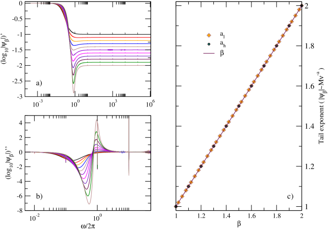
Figure 2: As in figure 1: a) Logarithmic derivative of $\log_{10}|\psi_{\beta}(\omega)|$ vs. $\log_{10}(\omega/2\pi)$. b) Logarithmic second derivative of $\log_{10}|\psi_{\beta}(\omega)|$ vs. $\log_{10}(\omega/2\pi)$. c) Exponent $a$ of tail for fitting $|\psi_{\beta}(\omega)|\sim\omega^{-a}$. Subindexes $l$ and $h$ refer to two different sampling ranges of medium and high frequencies, respectively. Solid line, again, signalizes ideal asymptotic tail $a\equiv\beta$. See text for explanations. $\beta>1$.

However some distinctions should be pointed out with the case $1<\beta\leq 2$, before to continue. Although both are the only ones with a positive density function of times of relaxation for all the stretched-squeezed exponentials [8, 9], $\exp(-t^{\beta})$, (i.e. with $\beta\in$$(0,\infty$)), they behave differently in the derivative and both show an obvious parametric discontinuity in the $t-$space. While for $\beta<1$ the minus derivative, $\beta t^{\beta-1}e^{-t^{\beta}}$, shows a singularity at $t=0$, the case $\beta>1$ presents a regular and continuous zero value though it pays the price of losing monotone decreasing behaviour of the former. Now it displays an increasing monotone growth and subsequently a decreasing monotone tail which saves the character of the positivity of the density function [8, 9]. They could be cases of a very different appearance or even to show a break in the continuity after doing the Fourier Transform for both but the real fact is that the parametric family of the first derivative transform, $\psi_{\beta}(\omega)$, does not present any oddity. Nonetheless the instance $\beta>1$ shows, truth is, a qualitatively different tail-to-body (i.e. tail to plateau and fall) response. While for the case $\text{$\beta$}<1$ the tail have the look of a natural extension of the fall, in the case $\beta>1$ there is an abrupt change of direction between the body fall at medium frequencies and the high frequency tail. We draw on to the representations of $(\log_{10}|\psi_{\beta}|)^{\prime}$ and $(\log_{10}|\psi_{\beta}|)^{\prime\prime}$ to explain the changes. (See figure 2). The first logarithmic derivative it is no longer a simple step, after the drop a narrow well is formed, (with the bottom at $\nu\lesssim 0.8$), and following this the line comes up and stabilizes at the selected value of $-\beta$, the same of the asymptote predicted by the series. What it is remarkable since the functional series from we obtained the expression for potential tail it is not converging in this case. (See figure 2a).

As a direct consequence of this new geometrical characteristic of the first derivative, the second logarithmic derivative presents two peaks, one negative and the other positive. The negative is a parametric continuation of the family shown for the case $\beta<1$, and has as a new property certain degree of skewness due to the presence of the second peak. Again the position of the maximum in OX axis grows in frequency and approaches to $\nu_{max}\lesssim 1$. It never reaches that ’high’ value for the interval $1\leq\beta\leq 2$, again because the second peak. The set of second peaks, looked at as a parametric family, accrues their maxima near to $\nu_{max}\sim 1$ as $\beta\rightarrow 2$. They are smaller than their corresponding partners. (See figure 2, there in the boxes of the first and second derivatives of $\log_{10}|\psi_{\beta}|$, for sake of clarity, are not depicted all the curves available but we have selected the last one of the previous group, $\beta=1$, the curves corresponding to $\beta=1.x0$ with $x\in$$\{1,2,...,9\}$ and $\text{$\beta$}=2.00$). The first peak corresponds to the fall of the body of the function $\log_{10}|\psi_{\beta}|$ and this one is even steeper than in the previous curves $\beta<1$ as the depth of the minimum grows in magnitude. The second peak, the positive, smaller in magnitude than the preceding negative, is a new phenomenology not seen in the previous case. It indicates a fold upwards in the curve $\log_{10}|\psi_{\beta}|$ in a very narrow region of frequencies as the short half-width of the peaks is developed in an interval with upper limit not beyond $\nu\sim 2$ as $\beta\rightarrow 2$. Of course for values of $\beta\lesssim 1.40$ the half-width is greater than this limit value but the height of the peak is so small compared to greater values of $\beta$ that the sidestep of the curve $\log_{10}|\psi_{\beta}|$ in this region is barely perceptible. (See figure 2b). Beyond this range of frequencies (i.e. $\nu\geq 10$) the ’activity’ of the second derivative, $(\log_{10}|\psi_{\beta}|)^{\prime\prime}$, is negligible and the function is mostly of a potential nature. In the figure 2c, as in the former case a graph of the exponent of tail vs. $\beta$ parameter is shown. We hold the same notation as before, $a_{l}$ for the result of the adjustment of $M\nu^{-a}$ to $\log_{10}|\psi_{\beta}|$, in the interval $\nu\in(20.0,500.0005]$ and $a_{h}$ for the fit in the range of $\text{$\nu$}\in(20.0,10^{7}]$. For the naked eye is quite difficult to distinguish the trend of these two sets of parameters from the result $a=\beta$, (solid line in the figure), what it points to an early high frequency tail very different in behaviour from the main body of the spectrum.

2 Common approaches

2.1 The asymptotic trends of 1-HN approximation

2.1.1 The stretched instance $\beta<1$

We have drawn two conclusions from the asymptotic behaviour of $|\psi_{\beta}|$. Firstly from a point of view of reconstruction in $t-$space only an small interval of low frequencies are needed to recover the main traits of the relaxation. Approximately the most significant part, –plateau, bend and fall–, happens in the range of $\nu\in[0,1]$ for most the betas and the tail almost stabilizes to its asymptotic functional form before $\nu<10$. And second this tail performs quite well as a potential decay of exponent $\beta$, i.e. $|\psi_{\beta}|\approx M\nu^{-\beta}$. Consequently, keeping in mind this two important features, and with the intention to design the best possible approximation, we shall test how the Havriliak-Negami function it sticks to the data, $|\psi_{\beta}|$, when we optimize the error between them. In short we wonder how the approximation in area distorts the desirable common path of the tails and reciprocally how the high frequency concomitance of the tails spoils the very low frequency description of a function, ($|\psi_{\beta}|$), which is steadier than its Havriliak-Negami alternate.

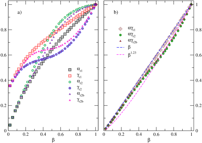
Figure 3: Left panel, a): Parameters $\alpha$ and $\gamma$ got from adjustment $\psi_{\beta}(\omega)\approx A*HN_{\alpha,\gamma}(\omega)$. The coarser step sampling, and $A\equiv 1$, is for mesh $r_{1}$. Finer steps are those of $r_{2}$, ($A\equiv 1$), and $r_{\text{2b}}$, $A\neq 1$). Right panel, b): Products $\alpha\cdot\gamma$ for the previous parameters. Dashed lines would correspond to situations $\alpha\cdot\gamma$$=\beta$ and $=\beta^{1.23}$.

To this end we made three related adjustments of the data in the interval $\nu\in[0,500.0005]$ to one Havriliak-Negami function. In the first case the sampling step in frequency interval was $\delta\nu=500/999.999$, that is a purged sample of the points used in the second and third cases, both with regular stride $\mbox{$\delta\nu$}=1/999.999$. Thus the influence of the body is practically eliminated and the tail is the responsible of the values of the parameters obtained for each beta. In the second case a standard fit is done, and in the third one the initial condition $HN_{\alpha,\gamma}(\omega=0)=1$ is relaxed to a free value, i.e. $\psi_{\beta}(\omega)\approx$ $A*HN_{\alpha,\gamma}(\omega)$ with $A$ to be determined in the optimization too. The idea behind this is to allow the Havriliak-Negami approximant compensates its lack of suitability in the very low frequencies, (there it doesn’t measure up, given its modulus is below $|\psi_{\beta}|$), and to soften the influence of the tail in relationship to the body part of data. The result, for $\beta<1$, points to the sensibility of $\alpha$ and $\gamma$ parameters to small changes in the approximation of $|\psi_{\beta}|$ area by $A*HN_{\alpha,\gamma}(\omega)$, –even with so small variations of $A$ as a maximum 6% around $\beta=0.32$–, and the sturdiness of tail influence on the asymptotic trend of $HN_{\alpha,\gamma}$.

In figure 3, to the left, we depict parameters $\alpha$ and $\gamma$ for the three referred cases, and in the right box the corresponding products $\alpha\cdot\gamma$ are graphed. In both boxes the subscripts $r_{1}$ are for the purged case, the $r_{2}$’s are for the common fit, $\psi_{\beta}\approx HN_{\alpha,\gamma}$, and the modified case $\psi_{\beta}\approx A*HN_{\alpha,\gamma}$ is denoted with $r_{2b}$.

We can see how $\alpha_{r1}(\beta)$ and $\gamma_{r1}(\beta)$ have a monotonous increasing behaviour and the curves only touch themselves at $\beta=1$. A changing picture when a finer mesh is used and the very low frequencies are added to the data, now the curves $\alpha_{r2}(\beta)$ and $\gamma_{r2}(\beta)$, still increasing ones that meet at $\beta=1$, cross one to the other within the interval (approx. at $0.32<\beta<0.35$). And the same happens to the extended approximation $A*HN_{\alpha,\gamma}$, though the crossover of $\alpha_{r2b}(\beta)$ and $\gamma_{r2b}(\beta)$ it is shifted to the right of the former ($0.42<\beta<0.45$). The $\alpha_{r?}(\beta)$ curves don’t change qualitatively, as their all first derivatives keep monotonously decreasing, but the $\gamma_{r?}(\beta)$’s do inasmuch as the first derivative suffers a transition from strictly decreasing function, ($r_{1}$), to one with a minimum (i.e. it decreases, halts and then increases for cases $r_{2}$ and $r_{2b}$). Besides for both families, $\alpha$ and $\gamma$, an apparent transition from $r_{1}$ to $r_{2}$ is observed in case $r_{2b}$. It suggests an enhancement of the weight of tail in detriment of plateau and fall weights, what it sounds logic insofar as the extended condition frees the constraint of approximating the low frequency zone by the correspondent region of Havriliak-Negami function, and this allows a greater influence on the remaining part by the data of high frequency. That is to say we do not provide to $HN_{\alpha,\gamma}(\omega)$ with a new functional flexibility, this should be achieved for example with additional terms, by contrast now the fit is obtained by coating, instead of adapting, the plateau of data. All this sets free the function tail to adapt itself to respective data tail. Consequently the appearance of transition that shows $r_{2b}$, stresses how carefully the design of the approximant, the method of optimization, the data absent of errors, and of course the frequency domain, should be done or chosen.

This is also seen in the graph of the tree products $\text{$\alpha$}\cdot\gamma_{r?}(\beta)$, (figure 3, right panel). The first one, $\alpha\cdot\gamma_{r1}$, follows heavily a straight line $y=\beta$, indeed a regression to $y=\beta^{a}$ gives $a=1.035$ with a correlation of $c.c.=0.999988$. The second and third cases ($r_{2}$ and $r_{2b}$), give $a=1.143$ with $c.c.=0.998633$ and $a=1.113$ with $c.c.=0.999004$ respectively. In all three cases the dependency deviates from proposed law $y=\beta^{1.23}$ [53, 70, 71], it is not much to say about $r_{1}$ since it holds data almost exclusively from tails, nevertheless $r_{2}$ and $r_{2b}$ maintain, by sampling, the information needed to reconstruct the original function to large times (i.e. low frequencies), and is quite significant that the approaching to the mentioned law is different according to the value $\beta$. When $0<\beta<0.6$ there is no closeness at all, and if $0.6<\beta<1.0$ the agreement is only due to the similar functional dependence, $\beta^{a}$. The point here is, as $\beta$ evolves from 0 to 1 the $(\log_{10}|\psi_{\beta}|)^{\prime}$ function takes form as an abrupt step which implies for $|\psi_{\beta}|$ a greater width for the plateau and a lesser magnitude and role for the tail, therefore while adjusting $\psi_{\beta}$ to a Havriliak-Negami function, a progression from tail dominated, ($y\sim m*\beta$, $m<1$), to body dominated fit, ($y\sim\beta^{a}$, $a>1$), will take place in product $\alpha\cdot\gamma(\beta)$. Logically this transition will be spoiled if the tails for small beta values does not develop properly and they are rounded off at the limits of an $\omega-$space finite interval, such thing happens for the FFT and is expected for an algorithm that erodes sharp characteristics whilst it determines the density of relaxation times [53, 89, 90]. In such circumstances each different procedure used will change the beta dependence of $\alpha\cdot\gamma$ in a particular and own way [49, 53, 70, 71].

Figure 4: Parameters, $\tau_{1,2}$ and $\lambda$ in the panel a, and in the b one $\alpha_{1,2}$ and $\gamma_{1,2}$, for an approximant $\mathcal{A}p_{2}HN_{\alpha,\gamma,\tau,\lambda}(\omega)$, as in Eq. 1, obtained adjusting the function to, ($r_{1}$), sampled data of $|\psi_{\beta}|$ in the range of medium frequencies. $\beta\leq 1$. Observe the similarities with a fit of same kind for high frequencies. Only $\lambda$ (medium) shows a behaviour more akin to low frequencies than to high ones. See figures 5 and 6. Dotted lines are just an aid for the eye.

2.1.2 The squeezed instance $\beta>1$

The linear approach to $\alpha\cdot\gamma(\beta)$ nevertheless fails, for same kind of samplings $r_{1}$, $r_{2}$ and $r_{2b}$, when $1<\beta<2$. In this region of control parameter $\beta$ a good empirical fitting will be $y=\beta$$+A_{1}(\beta-1)^{1.3}$$+A_{2}(\beta-1)^{3.7}$$+A_{3}(\beta-1)^{10}$ with a correlation of $0.999999$ for the three cases. Obviously the magnitude of parameters will vary being the look of $r_{1}$ different of $r_{2}$ or $r_{2b}$. While at first sight $r_{1}$ could seem a deviation from linearity easily corrected with a simple power of $(\beta-1)$ –it is possible to correct $y\sim\beta$ with a quadratic power to obtain a good agreement– the remaining two cases need more higher power terms to give the impression of a rapidly growing function. Besides in all cases $A_{i,r1}<<$$A_{i,r2b}<A_{i,r2}$, with $i=1,2,3$ and $A_{2}$ bigger than the other two $A^{\prime}s$, allowing the interpretation of $r_{2b}$ as an intermediate case between a tail dominant adjustment and a body dominant one. Exactly as in interval $0<\beta<1$, though with a great difference, the difficulty to obtain a behaviour that resembles the asymptotic trend of data $y\approx\beta$.

This hindrance should be borne in mind when making an approximation to $\psi_{\beta}$. As there is a sudden change of direction in the modulus from the dropping to the tail around $\nu\approx 1$ and a very fast decreasing of magnitude, any function showing monotony in decreasing and lack of oscillations or ripples will have large difficulties to follow the data from low to high frequencies. Therefore our choice, a description by a simple Havriliak-Negami approximant, won’t keep on track with tail inasmuch as the low frequency part of data is heavier and prevailing than the high frequency part and the fitting function too mild for dodging the twist presented by the second logarithmic derivative. Consequently, even when a residual quantity of data of such frequencies are present in the sample, the optimization process will balance towards a selection of parameters describing mainly the plateau and rise height of step rather than the tail. This is what happens with case $r_{1}$ which deviates from linearity $y=\beta$ and of course explains, when the whole sample of data is used in $r_{2}$ and $r_{2b}$, the explosion of product $\alpha\cdot\gamma(\beta)$, for $1<\beta<2$.

2.2 The asymptotic trends of 2-HN approximation

While the approximation of $\psi_{\beta}$ by means of one Havriliak-Negami function describes properly tail decaying of data for $\beta<1$, –although the asymptotic tendency of approximant suffers distortion because the matching to plateau zone–, it is clear from scientific literature that it is not enough to give an account of shape for the low frequencies [51, 53, 70, 87]. Neither is the case for $\beta>1$ as the advantage of picturing the high frequency asymptote is lost because tail weight in the optimization process can not offset plateau and drop predominance. However functional proximity can be improved adding a new H-N term for adapting to FFT of finite size temporal data [37, 53]. Is our intention to show that the same is true for the numerically calculated complex numbers $\psi_{\beta}(\omega)$ yet with an added feature, a right portrayal of the tail. Something that was not previously attained inasmuch as a finite window in the FFT distorted by convolution the high frequency part of spectrum. Our goal is then to show how this two terms approximant gives a good picture of both low and high frequencies. And how each term shares its contribution to the global approximation, a pertinent question because the roles of both terms will not be equal for cases $\beta<1$ and $\beta>1$.

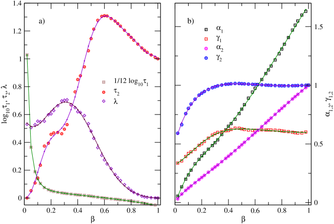
Figure 5: As in figure 4 parameters $\{\alpha_{1,2},\gamma_{1,2},\tau_{1,2},\lambda\}$ are calculated for a double approximant of Havriliak-Negami type. See Eq. 1. The frequency of data employed reaches up to $\nu\sim 10^{12}$ with $\beta\leq 1$. Lines are mathematical functions designed to describe these curves as dependent with variable $\beta$. See tables 1 and 2 in appendix.

2.2.1 The stretched case $\beta<1$

We have used the series of data till $\nu=500.0005$ in both versions $r_{2}$ (i.e. $\delta\nu_{r2}=1/999.999$), and $r_{1}$ ($\delta\nu_{r1}=500*\delta\nu_{r2}$) and the logarithmically homogeneous one $r_{sl}$ ($\delta\nu_{i,sl}=9*10^{a_{i}-3}$), until $\mbox{$\nu$}=10^{12}$, or $\mbox{$\nu$}=10^{7}$, for $\beta<1$ or $\beta>1$, respectively. The two terms approximant already described which will adjust data is

$$\mathcal{A}p_{2}HN_{\alpha,\gamma,\tau,\lambda}(\omega)=\sum_{s=1}^{2}\frac{\lambda_{s}}{(1+(i\tau_{s}\omega)^{\alpha_{s}})^{\gamma_{s}}}$$ (1)

with $\lambda_{1}\equiv\lambda$ and $\lambda_{1}+\lambda_{2}=1$.

Mesh sampling ($r_{1}$)

In figure 4 are presented the fitting parameters for case $r_{1}$ which is dominated by tail values in medium frequencies as the low frequencies are mainly absent by decimation. The right panel describes the responsible ones for the potential behaviour of tails, $\alpha_{1,2}$ and $\gamma_{1,2}$, and the left panel describes the characteristic times of both functions, $\tau_{1,2}$, plus share coefficient $\lambda$. In the left panel is convenient to take notice of a slowing varying lambda in interval $0.02\leq\beta\lesssim 0.6$ with a value near to 0.5 which suddenly drops to zero from $\beta\approx$ 0.60 to 1.00, also is remarkable the difference in magnitude between $\tau_{1}$ and $\tau_{2}$. While $\tau_{2}$ never exceeds the value of 1.1, $\tau_{1}$ requires of a decimal logarithmic scale to be shown in the same graph. It gives the idea of a dominant function associated with $\tau_{2}$ only corrected by the one associated with $\tau_{1}$ in the necessary zone of low frequencies, an oversimplified picture because is more accurate with values of $\beta$ near to 1.00 than with values near to 0.02 as both functions decay very slowly in this range of parameter $\beta$, due to small values of $\alpha_{1}$ and $\alpha_{2}$. However it is a good frame of reference to talk about the contribution of each $HN_{s=1,2}(\omega)$, so we’ll refer recurrently in these terms to them.

In the right panel two features should be noticed, first $\alpha_{2}$ and $\gamma_{2}$ do not cross one each other in line with what we saw while using only one Havriliak-Negami function to describe pruned data. And second in consonance with the fact that $\lambda$ diminishes in value approximating to zero and the numerical optimization is locked by only one $HN(\omega)$ function, $\alpha_{1}$ and $\gamma_{1}$ both present an apparent discontinuity at $\beta=1$. Although not all of these two functions is wrong as they cross themselves a property of $\alpha$ and $\gamma$ already shown in the case of approximating data, (low frequencies included), with only one Havriliak-Negami function. This fact enforces the idea of considering $HN_{1}(\omega)$ a backup for $HN_{2}(\omega)$ while fitting functions to data in low frequency zone. (See figure 4).

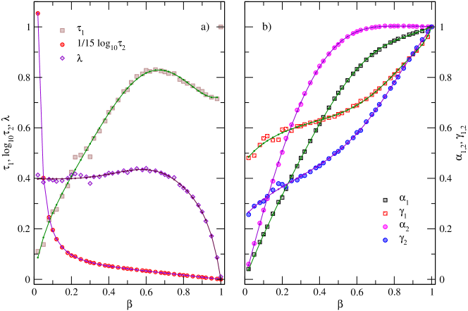
Figure 6: Parameters $\{\alpha_{1,2},\gamma_{1,2},\tau_{1,2},\lambda\}$ obtained after minimizing $\big{|}|\psi_{\beta}|-|\mathcal{A}p_{2}HN_{\alpha,\gamma,\tau,\lambda}(\omega)|\big{|}$ in the interval of frequencies $\nu\in[0,500.0005]$, with $\delta\nu=1/999.999$. $\beta\leq 1$. Solid lines are analytical rough estimates to describe the parameters. See tables 3 and 4 in appendix.

Mesh sampling ($r_{sl}$)

With the aim of testing this hypothesis, namely the residuary influence at low frequency of ancillary Havriliak-Negami function ($HN_{1}(\omega)$), a further adjustment to data with larger interval of frequencies is done. Now the sampling called logarithmically homogeneous, $r_{sl}$, is used as previous data have a very fine step $\delta\nu$, which makes computationally hard any optimization in a sensible amount of time. The interval of frequencies is now $\nu\in[1.00,10^{12}]$ for $\beta<1$ with the aforementioned step $\delta\nu_{i,sl}$ which changes in each decade of frequency. After calculations a new layout springs out as result for the parameters of approximant, this is shown in figure 5. We observe important differences, comparing to latter result, for every parameter. For share coefficient lambda the quick decreasing starts sooner, nearly $\beta\sim$ 0.4 and has opposite curvature to the prior case, besides the values attained in the interval $0<\beta\lesssim 0.4$ are comprised between 0.5 and 0.7 and do not seem steady as before. The curve for $\tau_{2}$ also suffers modifications, now is smoother and starts near zero for $\beta\sim 0$ and reaches one for $\beta=1$. This is in consonance with the errors and the final optimization for $r_{2}$ sampling case and suggests that the former curve for $r_{1}$ suffers from an strong source of error, possibly an interference between $HN_{1}(\omega)$ and $HN_{2}(\omega)$ in the initial interval $0.02\leq\beta<0.18$. A hint to explain such situation is to realize the opposite results of $\tau_{1}$ and $\alpha_{1}$. While $\tau_{1}$ would imply a very quick decay of $HN_{1}(\omega)$, the small value of $\alpha_{1}$ would slow down such decay, and would yield a non negligible contribution, something not to be expected from greater values of $\alpha_{1}$.

This balance allows a slight rivalry with the values of $HN_{2}(\omega)$ also dominated by a small $\alpha_{2}$. As a consequence of this equilibrium large fluctuations of $\tau_{2}$ in the neighborhood of $\beta\sim 0$ make sense. Finally we should add that interferences in the vicinity of $\beta\sim 1$ between $HN_{1}(\omega)$ and $HN_{2}(\omega)$ also occur affecting $\tau_{1}$, because for this curve a discontinuity happens at $\beta=1$ since $\tau_{1}(\beta=1)=1$ and $\tau_{1}(\beta\lesssim 1)<1$. And $\tau_{1}$ is not the only parameter with such discontinuity, $\alpha_{1}$ and $\gamma_{1}$ also take values quite far from their ideal amount of 1 near $\beta\lesssim 1$. (See figure 5). This pathology, partially consequence of a negligible $\lambda$, points to a minor and complementary role of $HN_{1}(\omega)$ describing $\psi_{\beta\lesssim 1}(\omega)$ tail. A trend which is the opposite when the beta values are small, as the change of almost every parameter curve in the neighborhood of $\beta\sim 0.4$ seems to suggest. It is worthy to note the coincidence of this turnaround with the fact the tails are not fully developed at very high frequencies for lesser values of beta than 0.4, at least when a comparison with greater values, (v. gr. $\beta>0.6$), is done. See figure 1, graph a. To finish we should like to remark the quasi constant behaviour of $\gamma_{1,2}$ in the interval $0.40\lesssim\beta<1$ and the quasilinear one of $\alpha_{1,2}$ in the whole interval of beta, making the relaxation of tails for $HN_{2}(\omega)$ nearer to a Cole-Cole type, ($\gamma\equiv 1$), than to a Cole-Davidson one, ($\alpha\equiv 1$). By contrast relaxation for $HN_{1}(\omega)$ still remains Havriliak-Negami in both cases $r_{1}$ and $r_{sl}$ though they are very different as a family of curves, (compare $\gamma_{1}$ in figures 4 and 5), inasmuch as $\gamma_{1}$ in $r_{1}$ is an increasing function for all the beta domain and $\gamma_{1}$ in $r_{sl}$ holds itself as quasi constant in the mentioned subinterval $\beta\in(0.4,1.0]$. Surely the lesser weight of medium and low frequencies in $r_{sl}$ with respect to $r_{1}$ takes its toll.

Mesh sampling ($r_{2}$)

Finally an adjustment to an $r_{2}$ sampling which includes many points corresponding to low frequencies is done, the result is that the roles of characteristics times $\tau_{1}$ and $\tau_{2}$ are interchanged. Now $\tau_{1}$ scale does not surpass the value of one. For betas near to one $\tau_{1}$ is around 0.7 and at $\beta=1$ is discontinuous, besides after a maximum located at $\beta\approx 0.62$ it decreases to 0.1 as $\beta\rightarrow 0.02$. Meanwhile $\tau_{2}$ is a monotonous decreasing curve from $\beta\sim 0$ to $\beta=1.00$ which can not be represented in the same scale as before unless decimal logarithms are taken and rescaling is done. (See left panel in figure 6). This suggests for the whole range of beta two scenarios, one in which the first term of the approximant, $HN_{1}(\omega)$, losses progressively importance as beta grows. It starts at $\beta\approx 0.62$ and ends when the approximant becomes degenerate $\mathcal{A}p_{2}HN_{\alpha,\gamma,\tau,\lambda\rightarrow 0}(\omega)\approx HN_{\{\alpha_{2},\gamma_{2},\tau_{2}\}\rightarrow\{1,1,1\}}(\omega)$, at $\beta=1.00$, (i.e. tends to a Debye relaxation as $\lambda\rightarrow 0$). This feature avoids the proper numerical determination of all parameters of $HN_{1}(\omega)$ and explain why $\tau_{1}$ is discontinuous, the optimization is locked by the suitability of $HN_{2}(\omega)$ and no further contribution of $HN_{1}(\omega)$ is possible. On the contrary, in the second scenario, ($0.02\leq\text{$\beta$}<0.62$), lambda, which takes values near to 0.4, shares out equal amount of contribution to each Havriliak-Negami term. Now the difference in contribution between both terms is due to the very distinct scale of time for $\tau_{1}$ and $\tau_{2}$, making one to be the complement of the other in this fit, while at the same time the tail asymptotic behaviour is mostly preserved. This situation allows to the approximant $\mathcal{A}p_{2}HN_{\alpha,\gamma,\tau,\lambda}(\omega)$ a description for a wide range of frequencies without excessive gap with data, $\psi_{\beta}(\omega)$. (See figure 9). Pairs $\alpha_{1},\gamma_{1}$ and $\alpha_{2},\gamma_{2}$ show a similar behaviour, –for each pair, the curves cross themselves and have similar shapes to the case of one Havriliak-Negami approximant (see figure 3)–, what is also consistent with a detailed description of plateau and drop, (i.e. the low frequencies), by jointly both Havriliak-Negami functions. (See right panel in figure 6).

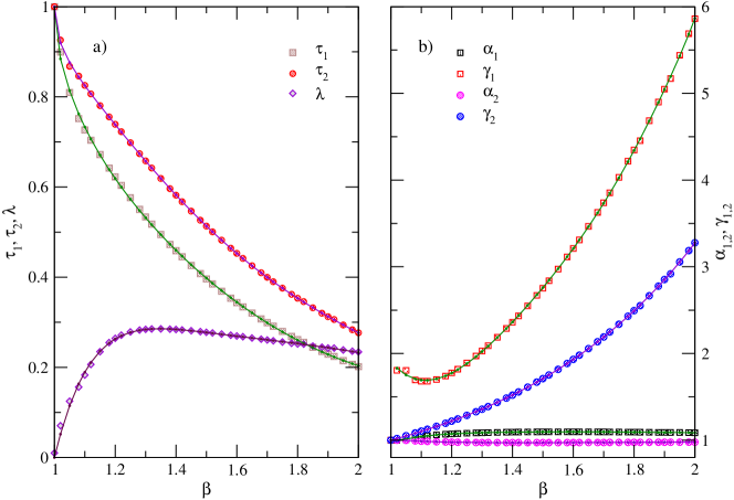
Figure 7: Parametric curves $\{\alpha_{1,2},\gamma_{1,2},\tau_{1,2},\lambda\}$ of a two-terms approximant, (see Eq. 1), for data, $|\psi_{\beta}|$, picked from interval $\nu\in[0,500.0005]$ with $\delta\nu=1/999.999$. $\beta\geq 1$. Solid lines are mathematical expressions tailored to adjust the curves. See tables 5 and 6 in appendix.

The empirical functions for the adjusting parameters $\alpha_{1,2}$, $\gamma_{1,2}$, $\tau_{1,2}$ and $\lambda$ are given in tables 1 and 2 for long frequency tails ($r_{sl}$), and in tables 3 and 4 for low to medium frequencies ($r_{2}$), all of them are written for interval $0<\beta\leq 1$ of control parameter.

2.2.2 The squeezed case $\beta>1$

However a different kind of results are obtained for the interval $1<\beta\leq 2$. We already pointed out how a sudden change in direction makes bend upwards the curve $|\psi_{\beta}(\omega)|$, which stabilizes in a potential tail at medium frequencies, after a very sharp dropping in the low to medium range of them. As a result the transition from plateau and rise height to tail is marked clearly by the decimal logarithmic curvature –which presents a chasm and a peak–, and consequently the adjustment to data by a Havriliak-Negami approximant is made more difficult, as the latter does not show such an extreme changes in curvature. The weight of low frequencies is bigger than the data corresponding to tail because their respective magnitude and total number of points, (for sampling $r_{2}$), thus the parameters obtained after optimization are those of a quick decaying function not following the natural asymptote. (See figure 7). Accordingly a global description of data would require necessarily a different two terms approximant of Havriliak-Negami type for the tail and every $\beta$. To obtain this we would proceed as before with an additional fit to a sampling like $r_{1}$ or $r_{sl}$ as both are pruned of low frequencies. In these cases they are sets of data weighting mostly the medium to high frequencies and the corresponding result will describe the tail asymptotic behaviour properly at the expense of not describing at all the plateau and its environs. Nevertheless the analysis $\alpha_{1,2}$, $\gamma_{1,2}$, $\tau_{1,2}$ and $\lambda$ as empirical functions of $\beta$ deals with remnant information of this neglected important part of the spectrum.

Figure 8: Parametric curves $\{\alpha_{1,2},\gamma_{1,2},\tau_{1,2},\lambda\}$ of an $\mathcal{A}p_{2}HN_{\alpha,\gamma,\tau,\lambda}$ function approximating data $|\psi_{\beta}|$ up to $\nu\sim 10^{7}$, in a homogeneous-like logarithmic pace. (See Eq. 1 and text). Notice the big dispersion of experimental points $\alpha_{1}$ and $\gamma_{1}$, and the correlated corresponding error of $\alpha_{2}$ and $\gamma_{2}$. It is remarkable that, even with this scattering of the parameters, the products $\alpha_{1}\cdot\gamma_{1}$ and $\alpha_{2}\cdot\gamma_{2}$ hold themselves extremely attached to a linear trend. (See figure 9c and d). Solid lines are rough proposals based on constraints given by same products. See tables 7 and 8 in appendix.

The triplet {$\alpha_{2}$, $\gamma_{2}$, $\tau_{2}$} is in both samplings, $r_{1}$ and $r_{sl}$, describable by means of smooth functions (v.gr. combination of exponentials and polynomials) and also is the case, except for some occasional dimple in $r_{sl}$, for the share coefficient $\lambda$. (See figure 8). Nonetheless it is not such a way for the triplet {$\alpha_{1}$, $\gamma_{1}$, $\tau_{1}$}. Though it could be possible to adjust $\tau_{1}$ with just one mathematical expression and the errors with data points wouldn’t be large, it won’t be the case for $\alpha_{1}$ and $\gamma_{1}$. (See right panel in figure 8). These last two curves are crooked, or even broken, in many points and do not show a defined trend, besides this happens for both cases $r_{1}$ and $r_{sl}$ but each in their own ways. Thus only a piecewise description is admissible for them. However this is not the treatment we are looking for the parameters as it would require an interpolating table, and certainly many errors, instead a simple formula. But not all is lost, paradoxically the product $\alpha_{1}\cdot\gamma_{1}$ is well behaved and can be fairly approximated to $\alpha_{1}\cdot\gamma_{1}\simeq 2\beta$ in case $r_{sl}$ and to $\alpha_{1}\cdot\gamma_{1}\simeq$ $-0.22+2.06\beta$ in case $r_{1}$. And meanwhile the product $\alpha_{2}\cdot\gamma_{2}$ is even closer and more correlated to a straight line, (i.e. $\alpha_{2}\cdot\gamma_{2}\simeq\beta$ with very small errors in both cases), than the previous product. The evident conclusion is that in spite of the bad conditioning and many errors finding $\alpha_{1}$ and $\gamma_{1}$ out the asymptotic tendency of tails is well described with a two-term Havriliak-Negami sum. On one side the second term, $HN_{2}(\omega)$, dictates the tail behaviour which at large $\nu$ coincides with the trend of real data, and on the other hand the first term, $HN_{1}(\omega)$, –quickly fading–, gives a proper placement of the curve near such data. And for this last constituent, notwithstanding the poorly defined trends of $\alpha-$ and $\gamma-$type parameters, the stability of constraint $\alpha_{1}\cdot\gamma_{1}\simeq 2\beta$ allows us to put forward an ’ansatz’ for their dependence on $\beta$, which finally enables a finer classification of high frequency spectral data. This will namely: $\alpha_{1,2}\sim\mathcal{O}(\beta)$, $\gamma_{1}\sim\mathcal{O}(2)$ and $\gamma_{2}\sim\mathcal{O}(1)$.

In Figure 9 all $\alpha\cdot\gamma$ products already commented for $0<\beta\leq 2$ are depicted. Subscripts numbers $1$ and $2$ stand for the first and second $HN_{?}(\omega)$ term in each approximant, and letters $h$ and $t$ describe the adjustment to $r_{2}$ and $r_{sl}$ samplings, respectively.

Also in tables 5, 6, 7 and 8 mathematical adjustments to parameters $\alpha_{1,2}$, $\gamma_{1,2}$, $\tau_{1,2}$ and $\lambda$ are recorded for $1<\beta\leq 2$. In table 5 and table 6 the formulae represent a quite close match to the empirical points which define the approximant for low frequencies, the counterpart for high frequencies is in tables 7 and 8. However in these last two tables the intended formulas for point curves $\alpha_{1}$, $\gamma_{1}$ and $\tau_{1}$ are just rough estimates as such curves show breaks and outliers. The remaining point graphs, (i.e. $\alpha_{2}$, $\gamma_{2}$, $\tau_{2}$ and $\lambda$), exhibit nevertheless an appropriate fit and as a consequence the mathematical expressions which substitute them give a good description of the high frequency behaviour (i.e. the asymptotes) although possibly with a misplacement due to errors describing the set of parameters {$\alpha_{1}$, $\gamma_{1}$, $\tau_{1}$}.

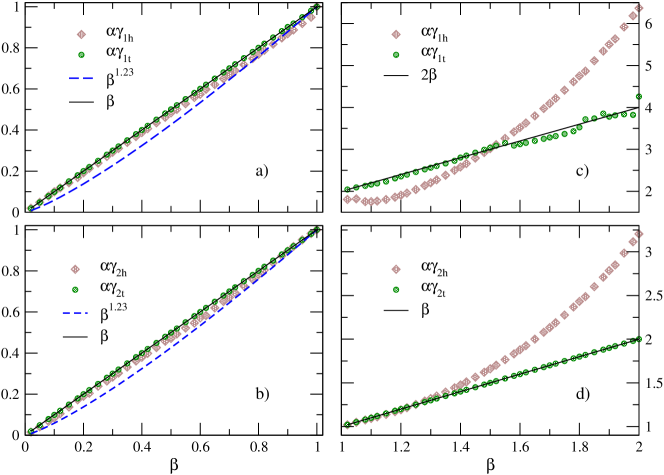
Figure 9: Products $\alpha_{1}\cdot\gamma_{1}$ and $\alpha_{2}\cdot\gamma_{2}$ of the asymptotic parameters, gotten by optimizing $\mathcal{A}p_{2}HN_{\alpha,\gamma,\tau,\lambda}\sim\psi_{\beta}$ in samplings $r_{2}$, –subindex $h$: head–, and $r_{sl}$, –subindex $t$: tail–, along the whole interval of variable $0<\beta\leq 2$. The solid line inside boxes a, b and d represents $\alpha\cdot\gamma=\beta$, while it is for $\alpha\cdot\gamma=2\beta$ in box c. In boxes a and b is also depicted the tendency $\alpha\cdot\gamma=\beta^{1.23}$ with a dashed line.

3 Discussion

By comparing the parametric curves $\{\alpha_{1,2},\gamma_{1,2},\tau_{1,2},\lambda\}$, (see figure 6), with those of a previous approximation to data $\psi_{\beta}(\omega)$ which undergo convolution with a sinc function, one can see a strong distortion in curves $\alpha_{1,2}$ and $\gamma_{1,2}$ for low values of $\beta\leq 1$. (See figures 3 and 4 in reference [53]). In that case they didn’t tend to zero as it happens in our present situation for $\alpha_{1,2}$, nor retained a value below 1 for $\gamma_{1}$, whithin an interval of small values of beta ($\beta<0.25$). And of course neither of them allowed us to consider constraints of type $(\alpha\cdot\gamma)_{1,2}\sim\mathcal{O}(\beta)$ as valid ones. However a successful reconstruction of the Kohlrausch function was still possible by means of inverse FFT for small ($\beta=0.15$) and large ($\beta=0.85$) values, despite these facts.

Some circumstances played a role to compensate the until then unknown distortion of beta-parametrized curves $\{\alpha,\gamma\}_{1,2}$. Among them: the serious problems in the medium-to-high frequencies interval, $\nu\in[10,500]$, were overcome easily with a proper damping of phase in the approximation, while the problems in low frequency range –consequence of discrepancy between data and the approximant pair– were shadowed by the finite size of time window through the smearing of peaks. Also the tails of both functions differed so slightly in a finite interval that made imperceptible the disagreements in reconstruction at short time scale.

Nevertheless what it was really good for the purpose of ignoring the distance in function space between the Fast Fourier Transform and the double Havriliak-Negami approximant, –i.e. its adaptability thanks to the many parameters–, played against a proper description of the theoretical Fourier Transform. The main three barriers cited which oppose to the perfect fit of HN approximant and FT data, will suffer dissimilar transformation through the process of convolution of data with a finite window, by the simple reason of being differently developed head, drop and tail along the same frequency interval. So, the change of shape induced by convolution, not only in plateaux but also in the tails where the potential behavior $\omega^{-\beta}$ was rounded due to finite size of spectrum, will be different with the value of $\beta$.

In consequence the functional dependence of $\{(\alpha,\gamma,\tau)_{1,2},\lambda\}(\beta)$ for the HN functions has to result distorted with respect to the desired result of same family while follows theoretical FT data. Such deviation will depend on $\beta$ inasmuch as the distortion of the FFT is not equally distributed with this parametric variable. Obviously a lesser drop tail-to-head in the functions with small $\beta$ values wore a greater adaptation of the approximants to the convolved data, loosing some of the original characteristics of theoretical data.

4 Conclusions

It is common practice while studying complex systems to analyze their relaxations in time as well as in frequency. Unfortunately there are not often at hand short and compact expressions corresponding simultaneously to the mathematical formulation of a same phenomenon in both spaces. This article is focused towards the approximation of Fourier Transform of certain Weibull distributions by Havriliak-Negami functions, studying their fitting instabilities and suitability. As the suggested models possess many parameters this first part delves thoroughly into the functional dependence of them with shape parameter $\beta$. Also we discuss the influence of data variation and extension on the resulting $\beta$ dependency, i. e. the sensibility of fit with data errors or distortions. Finally we will end this part establishing additional restrictions on parameter behaviour which are deduced from asymptotic trends of the theoretical functions.

When the values of $\psi_{\beta}(\omega)$ are sampled properly as to balance the weight of low frequency data with the more numerous and tiny values of high frequency tails during a fit or optimization, and besides such data are not distorted or biased by finite time windows in the Fourier transform of the original function $-\frac{d\exp(-t^{\beta})}{dt}$ or other numerical artifacts as consequence of switching from time to frequency space [53, 70, 89, 90], it will be true that a unique Havriliak-Negami function shall not follow other asymptotic condition $\alpha\cdot\gamma=\beta^{d}$ different of $d=1$.

Also whether two Havriliak-Negami functions are used as approximant the asymptotic constraints will be $(\alpha\cdot\gamma)_{1,2}=\beta$, for $\beta\leq 1$. While $(\alpha\cdot\gamma)_{1}\approx 2\beta$ and $(\alpha\cdot\gamma)_{2}=\beta$, for $2\geq\beta>1$. Nevertheless whenever the heads, ($\nu<1$), are involved and the tails, ($\nu>1$), are not sufficiently important to talk about a fully developed asymptotic trend, (see figures 1 and 2), the constraints for $\alpha\cdot\gamma$ won’t be fulfilled. In such cases $(\alpha\cdot\gamma)_{1,2}\sim\mathcal{O}(\beta)$ for $\beta\leq 1$, and $(\alpha\cdot\gamma)_{1,2}\sim\mathcal{O}(\beta^{d})$ with $d\geq 2$ for $\beta>1$.

These constraints should clear up our understanding of the fitting impediments found at low frequency while the model is being built. They suggest for slight changes in the uniform model of an approximant with two terms to give account of the whole range of frequencies. Unfortunately the accuracy of such approximations is restricted to the description of modulus of the objective function as far as our primary purpose is to understand the modifications required over HN functions to fit data in a better way. An additional work to fully optimize our models in the complex domain should be done by means of the information obtained from the new family of relaxation functions we have introduced here. Work is in progress towards such direction.

Appendix

Here are given the tables with formulae and parameter values corresponding to mathematical adjustments of point data in figures 5 to 8.

Case $0<\beta\leq 1$

Formulae	$\beta A\exp\big{[}(\sum_{s=1}^{3}a_{s}(1-\beta)^{s})\exp(-M\beta^{d})\big{]}$	$\frac{1}{A\exp\big{[}(\sum_{s=1}^{3}a_{s}(1-\beta)^{s})\exp(-M\beta^{d})\big{]}}$
$\frac{Parameters}{Constants}$ $A$ $M$ $d$ $a_{1}$ $a_{2}$ $a_{3}$ Corr.	$\alpha_{1}$ $\alpha_{2}$ 1.68125 $\equiv$1.000 6.00482 2.14961 0.712224 0.580585 -30.8645 0.56705 75.8761 -2.83736 -44.5841 2.97408 0.999858 0.999997	$\gamma_{1}$ $\gamma_{2}$ 1.6738 $\equiv$1.000 4.95993 2.49211 1.17881 0.651276 -5.87091 0.585986 13.4251 -2.92872 -6.94891 3.0715 0.997978 0.999256

Table 1: Approximant of tails, case $\beta\leq 1$: Formulas used to adjust $\{\alpha_{1,2},\gamma_{1,2}\}$ and their fitting constants [88]. Corr. = correlation coefficient of nonlinear fit. For $\alpha_{1}$ and $\gamma_{1}$, $\beta$=1 is an outlier. See right panel at figure 5.

Tables 1 and

$-0.65664+\dots$ $+\sum_{s=1}^{2}\big{\{}A_{s}(1-\beta)+B_{s}(1-\beta)^{2}\big{\}}\exp(-M_{s}\beta^{0.2})$	$\beta^{3}+\beta^{d}\sum_{s=1}^{7}b_{s}(1-\beta)^{s}$	$\exp(-M\beta^{d})\sum_{s=1}^{5}c_{s}(1-\beta)^{s}$
$\frac{Parameter}{Constants}$ $\log_{10}\tau_{1}$ $A_{1}$ -22.4446 $B_{1}$ -6.64276 $M_{1}$ -0.233028 $A_{2}$ 8231.54 $B_{2}$ -7799.77 $M_{2}$ 5.59666 Corr. 0.999984	$\frac{Parameter}{Constants}$ $\tau_{2}$ $d$ 2.96596 $b_{1}$ 4.54749 $b_{2}$ -32.4329 $b_{3}$ 552.577 $b_{4}$ -3159.47 $b_{5}$ 9513.52 $b_{6}$ -13492.1 $b_{7}$ 7139.92 Corr. 0.998613	$\frac{Parameter}{Constants}$ $\lambda$ $M$ 4.14933 $d$ 3.1579 $c_{1}$ 3.43714 $c_{2}$ -12.6851 $c_{3}$ 35.8224 $c_{4}$ -46.5211 $c_{5}$ 20.5172 Corr. 0.998905

Table 2: Approximant of tails, case $\beta\leq 1$: Formulas used to adjust $\{\tau_{1,2},\lambda\}$ and their fitting constants. Corr. = correlation coefficient of nonlinear fit. See left panel at figure 5.

2 describe a high frequency model and tables

Formulae	$\beta\exp\big{[}(\sum_{s=1}^{3}a_{s}(1-\beta)^{s})\exp(M\beta^{d})\big{]}$		$\frac{A}{\exp\big{[}(\sum_{s=1}^{3}a_{s}(1-\beta)^{s})\exp(M\beta^{d})\big{]}}$
$\frac{Parameters}{Constants}$ $M$ $d$ $a_{1}$ $a_{2}$ $a_{3}$ Corr.	$\alpha_{1}$ $\alpha_{2}$ 3.6903 2.42224 1.4618 1.03791 0.0190435 0.0962135 0.0794805 0.193794 0.572997 0.761107 0.999950 0.999942	$\frac{Parameters}{Constants}$ $M$ $d$ $A$ $a_{1}$ $a_{2}$ $a_{3}$ Corr.	$\gamma_{1}$ $\gamma_{2}$ 4.54457 3.4752 1.62482 1.47877 0.999202 1.00287 0.0227205 0.0401981 -0.055399 0.054449 0.79403 1.29633 0.998473 0.999654

Table 3: Approximant of heads, case $\beta\leq 1$: Formulas employed to adjust $\{\alpha_{1,2},\gamma_{1,2}\}$ and their fitting constants. Corr. = correlation coefficient. See figure 6.

3 and 4 do the same for a low frequency one.

$\beta^{d}\sum_{s=0}^{4}b_{s}(1-\beta)^{s}$	$\sum_{s=1}^{2}\big{\{}A_{s}(1-\beta)+B_{s}(1-\beta)^{2}\big{\}}\exp(-M_{s}\beta^{0.2})$	$\exp[-M(1-\beta)]\sum_{s=1}^{5}c_{s}(1-\beta)^{s}$
$\frac{Parameter}{Constants}$ $\tau_{1}$ $d$ 0.785731 $b_{0}$ 0.726519 $b_{1}$ 0.160075 $b_{2}$ 7.16583 $b_{3}$ -14.5815 $b_{4}$ 8.47342 Corr. 0.997479	$\frac{Parameter}{Constants}$ $\log_{10}\tau_{2}$ $A_{1}$ 42.4745 $B_{1}$ -49.3268 $M_{1}$ 3.65441 $A_{2}$ 66182.6 $B_{2}$ -61430.8 $M_{2}$ 12.7917 Corr. 0.999987	$\frac{Parameter}{Constants}$ $\lambda$ $M$ 4.60773 $c_{1}$ 4.80377 $c_{2}$ -12.6617 $c_{3}$ 78.3249 $c_{4}$ -120.494 $c_{5}$ 89.8475 Corr. 0.996847

Table 4: Approximant of heads, case $\beta\leq 1$: Formulas employed to adjust $\{\tau_{1,2},\lambda\}$ and their fitting constants. Corr. = correlation coefficient. See figure 6.

Case $2\geq\beta>1$

Formulae $1+\exp(\frac{-M}{\beta-1+\epsilon})\sum_{s=0}^{3}a_{s}(\beta-1)^{s},$ $\epsilon=10^{-180}.$ $A+\exp(M(\beta-1)^{3})\sum_{s=1}^{4}b_{s}(\beta-1)^{s}$ $\frac{Parameters}{Constants}$ $M$ $a_{0}$ $a_{1}$ $a_{2}$ $a_{3}$ Corr. $\alpha_{1}$ $\alpha_{2}$ 0.116811 0.165105 0.136577 -0.0645705 -0.0269458 0.0697225 -0.00692586 -0.0485374 -0.00572689 0.0171122 0.999249 0.999926 $\frac{Parameters}{Constants}$ $A$ $M$ $b_{1}$ $b_{2}$ $b_{3}$ $b_{4}$ Corr. $\gamma_{1}$ $\gamma_{2}$ 1.90381 $\equiv$1.000 2.25005 0.239754 -4.09964 0.948757 22.844 0.634155 -29.9149 0.692054 11.5881 -0.484575 0.999956 0.999993

Table 5: Approximant for heads, case $\beta>1$: Formulas used to adjust $\{\alpha_{1,2},\gamma_{1,2}\}$ and their fitting parameters. Corr. = correlation coefficient. The point at $\beta=1$ is an outlier for a fit to $\gamma_{1}$ and is removed. See figure 7.

Now the first pair of tables,

$c_{0}\sqrt{(\beta-1)}+\sum_{s=1}^{4}c_{s}(\beta-1)^{s}$	$\exp[-M(\beta-1)]\sum_{s=1}^{3}d_{s}(\beta-1)^{s}$
$\frac{Parameters}{Constants}$ $-\log_{10}\tau_{1}$ $-\log_{10}\tau_{2}$ $c_{0}$ 0.339472 0.27042 $c_{1}$ 0.27034 -0.1091 $c_{2}$ 0.0194173 0.977286 $c_{3}$ 0.26079 -0.884491 $c_{4}$ -0.198826 0.303991 Corr. 0.999853 0.999961	$\frac{Parameter}{Constants}$ $\lambda$ $M$ 2.9177 $d_{1}$ 2.80567 $d_{2}$ -3.18276 $d_{3}$ 4.6885 Corr. 0.998497

Table 6: Approximant for heads, case $\beta>1$: Formulas used to adjust $\{\tau_{1,2},\lambda\}$ and their fitting parameters. Corr. = correlation coefficient. See figure 7.

5 and 6, are those describing a two-function approximant in the domain of low frequencies, and tables

Formulae	$\beta\big{(}1+a_{1}(\beta-1)\big{)}$		$\frac{A}{\big{(}1+a_{1}(\beta-1)\big{)}}$
$\frac{Parameters}{Constants}$ $a_{1}$ Corr.	$\alpha_{1}$ $\alpha_{2}$ -0.127772 -0.00819886 0.981962 0.994925	$\frac{Parameters}{Constants}$ $A$ $a_{1}$ Corr.	$\gamma_{1}$ $\gamma_{2}$ $\equiv$2 $\equiv$1 -0.110735 -0.0102285 0.833974 0.096606!

Table 7: Approximant for tails, case $\beta>1$: Very rough trends decide formulas used to adjust $\{\alpha_{1,2},\gamma_{1,2}\}$ since noise is greater than signal at many points. The points at $\beta=$ 1.50, 1.52, 1.55, 1.80, 1.82 and 1.85 largely break the trend for a fit to $\alpha_{1}$ and $\gamma_{1}$ consequently they are removed. See figure 8. Notice the strong linear feature of products $(\alpha\cdot\gamma)_{1,2}$ despite the noise (see figure 9).

7 and 8 the corresponding to the high frequency model.

$B+b_{0}\sqrt{\beta-1}+\sum_{s=1}^{4}b_{s}(\beta-1)^{s}$ $\exp[-M\sqrt{\beta-1}]\sum_{s=1}^{3}c_{s}(\beta-1)^{s}$ $\frac{Parameters}{Constants}$ $-\log_{10}\tau_{1}$ $-\log_{10}\tau_{2}$ $A$ -0.278737 $\equiv$0 $b_{0}$ 1.69465 0.165075 $b_{1}$ -4.114 0.219429 $b_{2}$ 9.33908 1.33322 $b_{3}$ -10.9942 -2.39982 $b_{4}$ 4.63626 1.20034 Corr. 0.996880 0.999016 $\frac{Parameter}{Constants}$ $\lambda$ $M$ -0.504694 $c_{1}$ 1.41581 $c_{2}$ -1.49885 $c_{3}$ 0.572827 Corr. 0.998585

Table 8: Approximant for tails, case $\beta>1$: Formulas used to adjust $\{\tau_{1,2},\lambda\}$, and their fitting parameters. The points at $\beta=$ 1.12, 1.15, 1.78, 1.80, 1.82 and 1.85 are not taking into account while adjusting. See figure 8.

References

- [1] R. Kohlrausch, Pogg. Ann. Phys. Chem. 91, 56 (1854); 91, 179 (1854).
- [2] G. H. Hardy and J. E. Littlewood, Göttinger Nachrichten (Math. Phys. Klasse), 33 (1920).
- [3] W. R. Burwell, Proc. London Math. s2-22, 57 (1924).
- [4] N. G. Bakhoom, Proc. London Math. Soc. s2-35, 83 (1933).
- [5] V. Maric, Pub. de l’Institut Math. 13, 17 (1959).
- [6] D. Senouf, SIAM J. Math. Anal. 27, 1102 (1996).
- [7] J. Kamimoto, Kyushu J. Math. 52, 249 (1998).
- [8] S. Bochner, Duke Math. J. 3, 488 (1937).
- [9] S. Bochner, Duke Math. J. 3, 726 (1937).
- [10] A. Wintner, Duke Math. J. 8, 678 (1941).
- [11] P. Humbert, Bull. Sci. Math. 69, 121 (1945).
- [12] H. Pollard, Bull. Am. Math. Soc. 52, 908 (1946).
- [13] H. Bergstrom, Ark. Mat. 2, 375 (1952).
- [14] V. M. Zolotarev, One-Dimensional Stable Distributions, Russian Academy of Sciences - AMS, ISBN: 978-0-8218-4519-6 (1986).
- [15] A. Wintner, Ann. Math. Stat. 18, 589 (1947).
- [16] A. Wintner, Am. J. Math. 78, 819 (1956).
- [17] C. Fox, Proc. London Math. Soc. s2-27, 389 (1928).
- [18] W. G. Gloeckle and Th. F. Nonnenmacher, J. Stat. Phys. 71, 741 (1993).
- [19] A. C. Constantine and N. I. Robinson, Comp. Stat. & Data Anal. 24, 9 (1997).
- [20] R. Metzler, J. Klafter, J. Jortner, and M. Volk, Chem. Phys. Lett. 293, 477 (1998).
- [21] R. Hilfer, Phys. Rev. E 65, 061510 (2002).
- [22] J. Cheng, Ch. Tellambura, and N. C. Beaulieu, IEEE Trans. Comm. 52, 1265 (2004).
- [23] R. B. Paris, Eur. J. Pure Appl. Math. 3, 1006 (2010).
- [24] G. Williams and D. C. Watts, Trans. Faraday Soc. 66, 80 (1970).
- [25] G. Williams, D. C. Watts, S. B. Dev, and A. M. North, Trans. Faraday Soc. 67, 1323 (1971).
- [26] C. P. Lindsey and G. D. Patterson, J. Chem. Phys. 73, 3348 (1980).
- [27] J.-U. Hagenah, G. Meier, G. Fytas, and E. W. Fischer, Polymer J. 19, 441 (1987).
- [28] D. Boese, B. Momper, G. Meier, F. Kremer, J.-U. Hagenah, and E. W. Fischer, Macromolecules 22, 4416 (1989).
- [29] H. L. Lin, Y. S. Chen, and T. L. Yu, Polymer J. 26, 431 (1994).
- [30] K. C. Benny Lee, J. Siegel, S. E. D. Webb, S. Lévêque-Fort, M. J. Cole, R. Jones, K. Dowling, M. J. Lever, and P. M. W. French, Biophysical Journal 81, 1265 (2001).
- [31] M. N. Berberan-Santos, E. N. Bodunov, and B. Valeur, Chem. Phys. 315, 171 (2005).
- [32] M. N. Berberan-Santos, E. N. Bodunov, and B. Valeur, Chem. Phys. 317, 57 (2005).
- [33] S. Kuznetsova, G. Zauner, Th. J. Aartsma, H. Engelkam, N. Hatzakis, A. E. Rowan, R. J. M. Nolte, P. M. Christiansen, and G. W. Canters, Proc. Nat. Acad. Sci. 105, 3250 (2008).
- [34] J. C. Phillips, Rep. Prog. Phys. 59, 1133 (1996).
- [35] C. Hansen, R. Richert, and E. W. Fischer, J. Non-Cryst. Solids 215, 293 (1997).
- [36] P. G. Debenedetti and F. H. Stillinger, Nature 410, 259 (2001).
- [37] J. R. Macdonald and R. L. Hurt, J. Chem. Phys. 84, 496 (1986).
- [38] T. C. Halsey and Michael Leibig, Phys. Rev. A 43, 7087 (1991).
- [39] J. R. Macdonald, J. Non-Cryst. Solids 212, 95 (1997).
- [40] A. A. Gurtovenko and Yu. Ya. Gotlib, J. Chem. Phys. 115, 6785 (2001).
- [41] R. S. Anderssen, S. A. Husain, and R. J. Loy, ANZIAM J. 45, C800 (2004).
- [42] S. A. Baeurle, A. Hotta, and A. Gusev, Polymer 46, 4344 (2005).
- [43] F. Kohlrausch, Pogg. Ann. Phys. Chem. 119, 337 (1863).
- [44] E. W. Montroll and J. T. Bendler, J. Stat. Phys. 34, 129 (1984).
- [45] R. Boehmer, K. L. Ngai, C. A. Angell, and D. J. Plazek, J. Chem. Phys. 99, 4201 (1993).
- [46] P. Kaatz, P. Prêtre, U. Meier, U. Stalder, C. Bosshard, P. Günter, B. Zysset, M. Stähelin, M. Ahlheim, and F. Lehr, Macromolecules 29, 1666 (1996).
- [47] R. Ferguson, V. Arrighi, J. J. McEwen, S. Gagliardi, and A. Triolo, J. Macromol. Sci. Part B: Phys. 45, 1065 (2006).
- [48] M. T. Viciosa, G. Pires, J. J. Moura Ramos, Chem. Phys. 359, 156 (2009).
- [49] Ch. Schroeder and O. Steinhauser, J. Chem. Phys. 132, 244109 (2010).
- [50] S. H. Chung and J. R. Stevens, Am. J. Phys. 59, 1024 (1991).
- [51] G. H. Weiss, M. Dishon, A. M. Long, J. T. Bendler, A. A. Jones, P. T. Inglefield, and A. Bandis, Polymer 35, 1880 (1994).
- [52] K. M. Bennett, K. M. Schmainda, R. Bennett, D. B. Rowe, H. Lu, and J. S. Hyde, Magn. Reson. Med. 50, 727 (2003).
- [53] J.S. Medina, R. Prosmiti, P. Villareal, G. Delgado-Barrio, and J. V. Alemán, Phys. Rev. E 84, 066703 (2011).
- [54] J. Laherrère and D. Sornette, Eur. Phys. J. B 2, 525 (1998).
- [55] F. Wu and B. A. Huberman, Proc. Nat. Acad. Sci. 104, 17599 (2007).
- [56] H. K. Nakamura, M. Sasai, and M. Takano, Chem. Phys. 307, 259 (2004).
- [57] B. Fierz, H. Satzger, Ch. Root, P. Gilch, W. Zinth, and Th. Kiefhaber, Proc. Nat. Acad. Sci. 104, 2163 (2007).
- [58] H. Frauenfelder, G. Chen, J. Berendzen, P. W. Fenimore, H. Jansson, B. H. McMahon, I. R. Stroe, J. Swenson, and R. D. Young, Proc. Nat. Acad. Sci. 106, 5129 (2009).
- [59] A. R. Dobrovolskis, J. L. Alvarellos, J. J. Lissauer, Icarus 188, 481 (2007).
- [60] J. R. Macdonald, J. Appl. Phys. 62, R51(1987).
- [61] G. D. J. Phillies and P. Peczak, Macromolecules 21, 214 (1988).
- [62] H. Scher, M. F. Shlesinger, and J. T. Bendler, Physics Today 44, 26 (1991).
- [63] S. Sastry, P. G. Debenedetti, and F. Stillinger, Nature 393, 554 (1998).
- [64] K. Schroeter, R. Unger, S. Reissig, F. Garwe, S. Kahle, M. Beiner, and Donth, Macromolecules 31, 8966 (1998).
- [65] R. Kahlau, D. Kruk, Th. Blochowicz, V. N. Novikov, and E. A. Rössler, J. Phys.: Codens. Matter 22, 365101 (2010).
- [66] R. G. Palmer, D. L. Stein, E. Abrahams, and P. W. Anderson, Phys. Rev. Lett. 53, 958 (1984).
- [67] M. F. Shlesinger and E. W. Montroll, Proc. Natl. Acad. Sci. 81, 1280 (1984).
- [68] G. Williams, IEEE Trans. Electr. Insul. EI-20, 843 (1985).
- [69] K. Weron, A. Jurlewicz, M. Patyk, and A. Stanislavsky, Ann. Phys. 332, 90 (2013).
- [70] F. Alvarez, A. Alegria, and J. Colmenero, Phys. Rev. B 44, 7306 (1991).
- [71] F. Alvarez, A. Alegria, and J. Colmenero, Phys. Rev. B 47, 125 (1993).
- [72] S. Havriliak Jr. and S. J. Havriliak, Polymer 36, 2675 (1995).
- [73] H. Schaefer, E. Sternin, R. Stannarius, M. Arndt, and F. Kremer, Phys. Rev. L. 76, 2177 (1996).
- [74] R. Díaz-Calleja, Macromolecules 33, 8924 (2000).
- [75] J. Wuttke, preprint: arXiv:0911.4796v1, (2009); Algorithms 5, 604 (2012).
- [76] N. Koizumi and Y. Kita, Bull. Inst. Chem. Res. (Kyoto Univ.) 56, 300 (1978).
- [77] M. Dishon, G.H. Weiss, and J.T. Bendler, J. Res. Natl. Bur. Stand. 90, 27 (1985).
- [78] Ch. R. Snyder and F. I. Mopsik, Phys. Rev. B 60, 984 (1999).
- [79] E. Helfand, J.Chem. Phys. 78, 1931 (1983).
- [80] P. Debye, Ver. Deut. Phys. Gesell. 15, 777 (1913).
- [81] K. S. Cole and R. H. Cole, J. Phys. Chem. 9, 341 (1941).
- [82] D. W. Davidson and R. H. Cole, J. Chem. Phys. 19, 1484 (1951).
- [83] S. Havriliak and S. Negami, J. Polym. Sci. Part C 14, 99 (1966).
- [84] S. Havriliak and S. Negami, Polymer 8, 161 (1967).
- [85] W. Weibull, J. Appl. Mech. Trans. ASME. 18, 293 (1951).
- [86] H. Rinne, The Weibull distribution: A Handbook, CRC Press, ISBN: 978-1-4200-8743-7 (2009).
- [87] S. Havriliak Jr. and S. J. Havriliak, Polymer 37, 4107 (1996).
- [88] P. Turner, E. Stambulchik, and Grace Development Team, http://plasma-gate.weizmann.ac.il/Grace
- [89] S. W. Provencher, Comp. Phys. Comm. 27, 229 (1982).
- [90] Y. Imanishi, K. Adachi, and T. Kotaka, J. Chem. Phys. 89, 7593 (1988).