Evasion and Hardening of Tree Ensemble Classifiers

Abstract

Classifier evasion consists in finding for a given instance $x$ the “nearest” instance $x^{\prime}$ such that the classifier predictions of $x$ and $x^{\prime}$ are different. We present two novel algorithms for systematically computing evasions for tree ensembles such as boosted trees and random forests. Our first algorithm uses a Mixed Integer Linear Program solver and finds the optimal evading instance under an expressive set of constraints. Our second algorithm trades off optimality for speed by using symbolic prediction, a novel algorithm for fast finite differences on tree ensembles. On a digit recognition task, we demonstrate that both gradient boosted trees and random forests are extremely susceptible to evasions. Finally, we harden a boosted tree model without loss of predictive accuracy by augmenting the training set of each boosting round with evading instances, a technique we call adversarial boosting.

1 Introduction

Deep neural networks (DNN) represent a prominent success of machine learning. These models can successfully and accurately address difficult learning problems, including classification of audio, video, and natural language possible where previous approaches have failed. Yet, the existence of evading instances for the current incarnation of DNNs (Szegedy et al., 2013) shows a perhaps surprising brittleness: for virtually any instance $x$ that the model classifies correctly, it is possible to find a negligible perturbation $\delta$ such that $x+\delta$ evades being correctly classified, that is, receives a (sometimes widely) inaccurate prediction.

The general study of the evasion problem matters on both conceptual and practical grounds. First, we expect a high-performance learning algorithm to generalize well and be hard to evade: only a “large enough” perturbation $\delta$ should be able to alter its decision. The existence of small-$\delta$ evading instances shows a defect in the generalization ability of the model, and hints at improper model class and/or insufficient regularization. Second, machine learning is becoming the workhorse of security-oriented applications, the most prominent example being unwanted content filtering. In those applications, the attacker has a large incentive for finding evading instances. For example, spammers look for small, cost-effective changes to their online content to avoid detection and removal.

While prior work extensively studies the evasion problem on differentiable models by means of gradient descent, those results are reported in an essentially qualitative fashion, implicitly defaulting the choice of metric for measuring $\delta$ to the $L_{2}$ norm. Further, non-differentiable, non-continuous models have received very little attention. Tree sum-ensembles as produced by boosting or bagging are perhaps the most important models from this class as they are often able to achieve competitive performance and enjoy good adoption rates in both industrial and academic contexts.

In this paper, we develop two novel exact and approximate evasion algorithms for sum-ensemble of trees. Our exact (or optimal) evasion algorithm computes the smallest $\delta$ according to the $L_{p}$ norm for $p=0,1,2,\infty$ such that the model misclassifies $x+\delta$. The algorithm relies on a Mixed Integer Linear Program solver and enables precise quantitative robustness statements. We benchmark the robustness of boosted trees and random forests on a concrete handwritten digit classification task by comparing the minimal required perturbation $\delta$ across many representative models. Those models include $L_{1}$ and $L_{2}$ regularized logistic regression, max-ensemble of linear classifiers (shallow max-out network), a 3-layer deep neural network and a classic RBF-SVM. The comparison shows that for this task, despite their competitive accuracies, tree ensembles are consistently the most brittle models across the board.

Finally, our approximate evasion algorithm is based on symbolic prediction, a fast and novel method for computing finite differences for tree ensemble models. We use this method for generating more than 11 million synthetic confusing instances and incorporate those during gradient boosting in an approach we call adversarial boosting. This technique produces a hardened model which is significantly harder to evade without loss of accuracy.

2 Related Work

From the onset of the adversarial machine learning subfield, evasion is recognized as part of the larger family of attacks occurring at inference time: exploratory attacks (Barreno et al., 2006). While there is a prolific literature considering the evasion of linear or otherwise differentiable models (Dalvi et al., 2004; L., 2005; Lowd & Meek, 2005; Nelson et al., 2012; Brückner et al., 2012; Fawzi et al., 2014; Biggio et al., 2013; Szegedy et al., 2013; Srndic & Laskov, 2014), we are only aware of a single paper tackling the case of tree ensembles. In Xu et al. (Xu et al., 2016), the authors present a genetic algorithm for finding malicious PDF instances which evade detection.

In this paper, we forgo application-specific feature extraction and directly work in feature space. We briefly discuss strategies for modeling the feature extraction step in paragraph additional constraints of section 4.3. We deliberately do not limit the amount of information available for carrying out evasion. In this paper, our goal is to establish the intrinsic evasion robustness of the machine learning models themselves, and thus provide a guaranteed worst-case lower-bound. In contrast to (Xu et al., 2016), our exact algorithm guarantees optimality of the solution, and our approximate algorithm performs a fast coordinate descent without the additional tuning and hyper-parameters that a genetic algorithm requires.

We contrast our paper with a few related papers on deep neural networks, as these are the closest in spirit to the ideas developed here. Goodfellow et al. (Goodfellow et al., 2014) hypothesize that evasion in practical deep neural networks is possible because these models are locally linear. However, this paper demonstrates that despite their extreme non-linearity, boosted trees are even more susceptible to evasion than neural networks. On the hardening side, Goodfellow et al. (Goodfellow et al., 2014) introduce a regularization penalty term which simulates the presence of evading instances at training time, and show limited improvements in both test accuracy and robustness. Gu et al. (Gu & Rigazio, 2015) show preliminary results by augmenting deep neural networks with a pre-filtering layer based on a form of contractive auto-encoding. Most recently, Papernot et al. (Papernot et al., 2015) shows the strong positive effect of distillation on evasion robustness for neural networks. In this paper, we demonstrate a large increase in robustness for a boosted tree model hardened by adversarial boosting. We empirically show that our method does not degrade accuracy and creates the most robust model in our benchmark problem.

3 The Optimal Evasion Problem

In this section, we formally introduce the optimal evasion problem and briefly discuss its relevance to adversarial machine learning. We follow the definition of (Biggio et al., 2013). Let $c:\mathcal{X}\rightarrow\mathcal{Y}$ be a classifier. For a given instance $x\in\mathcal{X}$ and a given “distance” function $d:\mathcal{X}\times\mathcal{X}\rightarrow\mathbb{R}_{+}$, the optimal evasion problem is defined as:

$$\underset{x^{\prime}\in\mathcal{X}}{\text{minimize}}\;d(x,x^{\prime})\quad\text{subject to}\;c(x)\neq c(x^{\prime})$$ (1)

In this paper, we focus on binary classifiers defined over an $n$-dimensional feature space, that is $\mathcal{Y}=\{-1,1\}$ and $\mathcal{X}\subset\mathbb{R}^{n}$.

Setting the classifier $c$ aside, the distance function $d$ fully specifies (1), hence we talk about $d$-evading instances, or $d$-robustness. In fact, many problems of interest in adversarial machine learning fit under formulation (1) with a judicious choice for $d$. In the adversarial learning perspective, $d$ can be used to model the cost the attacker has to pay for changing her initial instance $x$. In this paper, we proceed as if this cost is decomposable over the feature dimensions. In particular, we present results for four representative distances. We briefly describe those and their typical effects on the solution of (1).

The $L_{0}$ distance

$\sum_{i=1}^{n}\mathbb{I}_{x_{i}\neq x^{\prime}_{i}}$, or Hamming distance encourages the sparsest, most localized deformations with arbitrary magnitude. Our optimal evasion algorithm can also handle the case of non-uniform costs over features. This situation corresponds to minimizing $\sum_{i=1}^{n}\alpha_{i}\mathbb{I}_{x_{i}\neq x^{\prime}_{i}}$ where $\alpha_{i}$ are non-negative weights.

The $L_{1}$ distance

$\sum_{i=1}^{n}|x_{i}-x^{\prime}_{i}|$ encourages localized deformations and additionally controls for their magnitude.

The $L_{2}$ distance

$\sqrt{\sum_{i=1}^{n}(x_{i}-x^{\prime}_{i})^{2}}$ encourages less localized but small deformations.

The $L_{\infty}$ distance

$\max_{i}|x_{i}-x^{\prime}_{i}|$ encourages uniformly spread deformations with the smallest possible magnitude.

Note that for binary-valued features, $L_{1}$ and $L_{2}$ reduce to $L_{0}$ and $L_{\infty}$ results in the trivial solution value 1 for (1).

4 Evading Tree Ensemble Models

We start by introducing tree ensemble models along with some useful notation. We then describe our optimal and approximate algorithms for generating evading instances on sum-ensembles of trees.

4.1 Tree Ensembles

A sum-ensemble of trees model $f:\mathbb{R}^{n}\rightarrow\mathbb{R}$ consists of a set $\mathcal{T}$ of regression trees. Without loss of generality, a regression tree $T\in\mathcal{T}$ is a binary tree where each internal node $n\in T.\text{nodes}$ holds a logical predicate $n.\text{predicate}$ over the feature variables, outgoing node edges are by convention labeled $n.\text{true}$ and $n.\text{false}$ and finally each leaf $l\in T.\text{leaves}$ holds a numerical value $l.\text{prediction}\in\mathbb{R}$. For a given instance $x\in\mathbb{R}^{n}$, the prediction path in $T$ is the path from the tree root to a leaf such that for each internal node $n$ in the path, $n.\text{true}$ is also in the path if and only if $n.\text{predicate}$ is true. The prediction of tree $T$ is the leaf value of the prediction path. Finally, the signed margin prediction $f(x)$ of the ensemble model is the sum of all individual tree predictions and the predicted label is obtained by thresholding, with the threshold value commonly fixed at zero: $c(x)=1\Leftrightarrow f(x)>0$.

In this paper, we consider the case of single-feature threshold predicates of the form $x_{i}<\tau$ or equivalently $x_{i}>\tau$, where $0\leq i<n$ and $\tau\in\mathbb{R}$ are fixed model parameters. This restriction excludes oblique decision trees where predicates simultaneously involve several feature variables. We however note that oblique trees are seldom used in ensemble classifiers, partially because of their relatively high construction cost and complexity (Norouzi et al., 2015). Before describing our generic approach for solving the optimal evasion problem, we first state a simple worst-case complexity result for problem (1).

4.2 Theoretical Hardness of Evasion

For a given tree ensemble model $f$, finding an $x\in\mathbb{R}^{n}$ such that $f(x)>0$ (or $f(x)<0$ without loss of generality) is NP-complete. That is, irrespectively of the choice for $d$, the optimal evasion problem (1) requires solving an NP-complete feasibility subproblem.

We now give a proof of this fact by reduction from 3-SAT. First, given an instance $x$, computing the sign of $f(x)$ can be done in time at most proportional to the model size. Thus the feasibility problem is in NP. It is further NP-complete by a linear time reduction from 3-SAT as follows. We encode in $x$ the assignment of values to the variables of the 3-SAT instance $S$. By convention, we choose $x_{i}>0.5$ if and only if variable $i$ is set to true in $S$. Next, we construct $f$ by arranging each clause of $S$ as a binary regression tree. Each regression tree has exactly one internal node per level, one for each variable appearing in the clause. Each internal node holds a predicate of the form $x_{i}>0.5$ where $i$ is a clause variable. The nodes are arranged such that there exists a unique prediction path corresponding to the falseness of the clause. For this path, the prediction value of the leaf is set to the opposite of the number of clauses in $S$, which is also the number of trees in the reduction. The remaining leaves predictions are set to 1. Figure 1 illustrates this construction on an example.

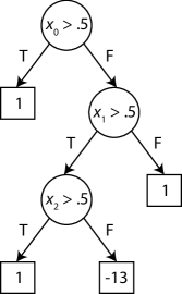
Figure 1: Regression tree for the clause $x_{0}\vee\neg x_{1}\vee x_{2}$. In this example, $S$ has 13 clauses.

It is easy to see that $S$ is satisfiable if and only if there exists $x$ such that $f(x)>0$. Indeed, a satisfying assignment for $S$ corresponds to $x$ such that $f(x)=|\mathcal{T}|>0$ and any non-satisfying assignment for $S$ corresponds to $x$ such that $f(x)\leq-1<0$ because there is at least one false clause which corresponds to a regression tree which output is $-|\mathcal{T}|$.

While we can not expect an efficient algorithm for solving all instances of problem (1) unless $\text{P}=\text{NP}$, it may be the case that tree ensemble models as produced by common learners such as gradient boosting or random forests are practically easy to evade. We now turn to an algorithm for optimally solving the evasion problem when $d$ is one of the distances presented in section 3.

4.3 Optimal Evasion

Let $f$ be a sum-ensemble of trees as defined in 4.1 and $x\in\mathbb{R}^{n}$ an initial instance. We present a reduction of problem (1) into a Mixed Integer Linear Program (MILP). This reduction avoids introducing constraints with so called “big-M” constants (Griva et al., 2008) at the cost of a slightly more complex solution encoding. We experimentally find that our reduction produces tight formulations and acceptable running times for all common models $f$.

In what follows, we present the mixed integer program by defining three groups of MILP variables: the predicate variables encode the state (true or false) of all predicates, the leaf variables encode which prediction leaf is active in each tree, and the optional objective variable for the case where $d$ is the $L_{\infty}$ norm.

We then introduce three families of constraints: the predicates consistency constraints enforce the logical consistency between predicates, the leaves consistency constraints enforce the logical consistency between prediction leaves and predicates, and the model mislabel constraint enforces the condition $c(x)\neq c(x^{\prime})$, or equivalently that $f(x^{\prime})>0$ or $f(x^{\prime})<0$ depending on the sign of $f(x)$. Finally we reduce the objective of (1) by relating the predicate variables to the value of $d(x,x^{\prime})$ in objective.

Program Variables

For clarity, MILP variables are bolded and italicized throughout. Our reduction uses three families of variables.

• At most $\sum_{T\in\mathcal{T}}|T.\text{nodes}|$ binary variables $\textit{{p}}_{i}\in\{0;1\}$ (predicates) encoding the state of the predicates. Our implementation sparingly create those variables: if any two or more predicates in the model are logically equivalent, their state is represented by a single variable. For example, the state of $x^{\prime}_{5}<0$ and $-x^{\prime}_{5}>0$ would be represented by the same variable.

• $\sum_{T\in\mathcal{T}}|T.\text{leaves}|$ continuous variables $0\leq\textit{{l}}_{i}\leq 1$ (leaves) encoding which prediction leaf is active in each tree. The MILP constraints force exactly one $\textit{{l}}_{i}$ per tree to be non-zero with $\textit{{l}}_{i}=1$. The l variables are thus implied binary in any solution but are nonetheless typed continuous to narrow down the choice of branching variable candidates during branch-and-bound, and hence improve solving time.

• At most 1 non-negative continuous variable b (bound) for expressing the distance $d(x,x^{\prime})$ of problem (1) when $d$ is the $L_{\infty}$ distance. This variable is first used in the objective paragraph.

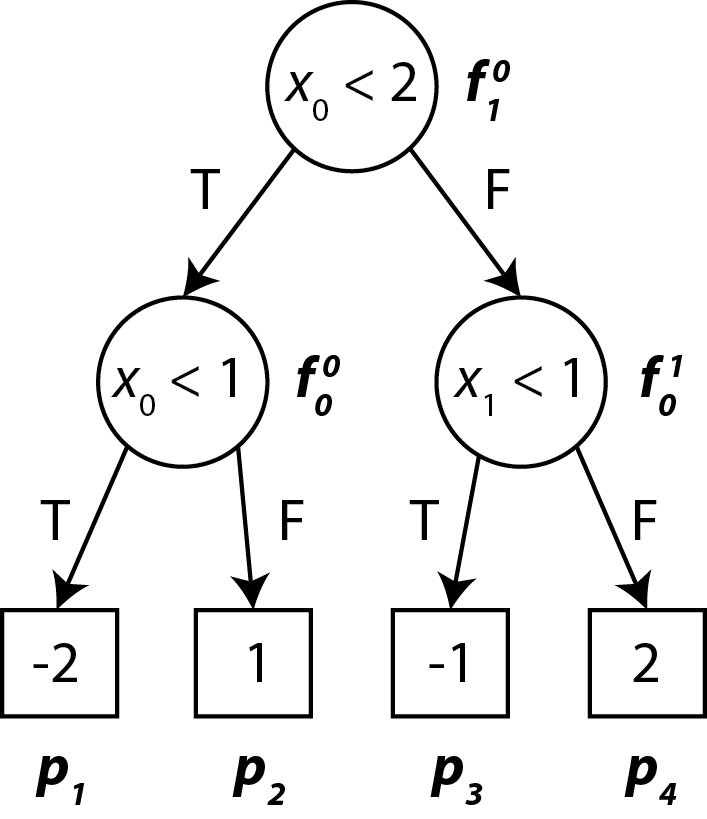
Figure 2: Regression tree for the reduction example. Predicate variables p and leaf variables l are shown next to their corresponding internal and leaf nodes. There are $n=2$ continuous features. The leaf predictions are -2, 1, 1 and 2.

In what follows, we illustrate our reduction by using a model with a single regression tree as represented in figure 2.

Predicates consistency

Without loss of generality, each predicate variable $\textit{{p}}_{i}$ corresponds to the state of a predicate of the form $x_{k}<\tau_{k}$. If two variables $\textit{{p}}_{i}$ and $\textit{{p}}_{j}$ correspond to predicates over the same variable $x_{k}<\tau_{1}$ and $x_{k}<\tau_{2}$, then $\textit{{p}}_{i}$ and $\textit{{p}}_{j}$ can take inconsistent values without additional constraints. For instance, if $\tau_{1}<\tau_{2}$, then $\textit{{p}}_{i}=1$ and $\textit{{p}}_{j}=0$ would be logically inconsistent because $x_{k}<\tau_{1}\Rightarrow x_{k}<\tau_{2}$, but any other valuation is possible.

For each feature variable $x^{\prime}_{k}$, we can ensure the consistency of all p variables which reference a predicate over $x^{\prime}_{k}$ by adding $K-1$ inequalities enforcing the implicit implication constraints between the predicates, where $K$ is the number of p variables referencing $x_{k}$. For a given $x^{\prime}_{k}$, let $\tau_{1}<\dots<\tau_{K}$ be the sorted thresholds of the predicates over $x^{\prime}_{k}$. Let $\textit{{p}}_{1},\dots,\textit{{p}}_{K}$ be the MILP variables corresponding to predicates $x^{\prime}_{k}<\tau_{1},\dots,x^{\prime}_{k}<\tau_{K}$. A valuation of $(\textit{{p}}_{i})_{i=1..K}$ is consistent if and only if $\textit{{p}}_{1}=1\Rightarrow\dots\Rightarrow\textit{{p}}_{K}=1$. Thus the consistency constraints are:

$$\textit{{p}}_{1}\leq\textit{{p}}_{2}\leq\dots\leq\textit{{p}}_{K}$$

When the feature variables $x^{\prime}_{k}$ are binary-valued, there is a single $\textit{{p}}_{i}$ variable associated to a feature variable: all predicates $x^{\prime}_{k}<\tau$ with $0<\tau<1$ are equivalent. Generally, tree building packages generate a threshold of $0.5$ in this situation. This is however implementation dependent and we can simplify the formulation with additional knowledge of the value domain $x^{\prime}_{k}$ is allowed to take.

In our toy example in figure 2, variables $\textit{{p}}_{0}$ and $\textit{{p}}_{1}$ refer to the same feature dimension $0$ and are not independent. The predicate consistency constraint in this case is:

$$\textit{{p}}_{1}\leq\textit{{p}}_{0}$$

and no other predicate consistency constraint is needed.

Leaves consistency

These constraints bind the p and l variables so that the semantics of the regression trees are preserved. Each regression tree has its own independent set of leaves consistency constraints. We construct the constraints such that the following properties hold:

1. if $\textit{{l}}_{k}=1$, then every other $\textit{{l}}_{i\neq k}$ variable within the same tree is zero, and

2. if a leaf variable $\textit{{l}}_{k}$ is 1, then all predicate variables $\textit{{p}}_{i}$ encountered in the prediction path of the corresponding leaf are forced to be either 0 or 1 in accordance with the semantics of the prediction path, and

3. exactly one $\textit{{l}}_{k}$ variable per tree is equal to 1. This property is needed because (i) does not force any $\textit{{l}}_{i}$ to be non-zero.

Enforcing property (i) is done using a classic exclusion constraint. If $\textit{{l}}_{1},\dots,\textit{{l}}_{K}$ are the $K$ leaf variables for a given tree, then the following equality constraint enforces (i):

$$\textit{{l}}_{1}+\textit{{l}}_{2}+\dots+\textit{{l}}_{K}=1$$ (2)

For our toy example, this constraint is:

$$\textit{{l}}_{1}+\textit{{l}}_{2}+\textit{{l}}_{3}+\textit{{l}}_{4}=1$$

Enforcing property (ii) requires two constraints per internal node. Let us start at the root node $r$. Let $\textit{{p}}_{\text{root}}$ be the variable corresponding to the root predicate. Let $\textit{{l}}^{T}_{1},\dots,\textit{{l}}^{T}_{i}$ be the variables corresponding to the leaves of the subtree rooted at $r.\text{true}$, and $\textit{{l}}^{F}_{1},\dots,\textit{{l}}^{F}_{j}$ the variables for the subtree rooted at $r.\text{false}$. The root predicate is true if and only if the active prediction leaf belongs to the subtree rooted at $r.\text{true}$. In terms of the MILP reduction, this means that $\textit{{p}}_{\text{root}}$ is equal to 1 if and only if one of the leaf variables of the true subtree is set to one. Similarly on the false subtree, $\textit{{p}}_{\text{root}}$ is 0 if and only if one of the leaf variables of the false subtree is set to one. Because only one leaf can be non-zero, these constraints can be written as:

$$1-\left(\textit{{l}}^{F}_{1}+\textit{{l}}^{F}_{2}+\dots+\textit{{l}}^{F}_{j}\right)=\textit{{p}}_{\text{root}}=\textit{{l}}^{T}_{1}+\textit{{l}}^{T}_{2}+\dots+\textit{{l}}^{T}_{i}$$

The case of internal nodes is identical, except that if and only ifs are weakened to single side implications. Indeed, unlike the root case, it is possible that no leaf in either subtree might be an active prediction leaf. For an internal node $n$, let $\textit{{p}}_{\text{node}}$ be the variable attached to the node, $\textit{{l}}^{T}$ and $\textit{{l}}^{F}$ the variables attached to leaves of the true and false subtrees rooted at $n.\text{true}$ and $n.\text{false}$. The constraints are:

$$1-\left(\textit{{l}}^{F}_{1}+\textit{{l}}^{F}_{2}+\dots+\textit{{l}}^{F}_{j}\right)\geq\textit{{p}}_{\text{node}}\geq\textit{{l}}^{T}_{1}+\textit{{l}}^{T}_{2}+\dots+\textit{{l}}^{T}_{i}$$

In our toy example, we have 3 internal nodes and thus six constraints. The constraints associated with the root, the leftmost and rightmost internal nodes are respectively:

$$\textit{{l}}_{1}+\textit{{l}}_{2} =\textit{{p}}_{0}=1-\left(\textit{{l}}_{3}+\textit{{l}}_{4}\right)$$

$$\textit{{l}}_{1} \leq\textit{{p}}_{1}\leq 1-\textit{{l}}_{2}$$

$$\textit{{l}}_{3} \leq\textit{{p}}_{2}\leq 1-\textit{{l}}_{4}$$

Finally, property (iii) automatically holds given the previously defined constraints. To see this, one can walk down the prediction path defined by the p variables and notice that at each level, the leaves values of one of the subtree rooted at the current node must be all zero. For instance, if $\textit{{p}}_{\text{node}}=1$, then we have

$$\textit{{l}}^{F}_{1}+\textit{{l}}^{F}_{2}+\dots+\textit{{l}}^{F}_{j}\leq 0\Rightarrow\textit{{l}}^{F}_{1}=\textit{{l}}^{F}_{2}=\dots=\textit{{l}}^{F}_{j}=0$$

At the last internal node, exactly two leaf variables remain unconstrained, and one of them is pushed to zero. By the exclusion constraint (2), the remaining leaf variable must be set to 1.

Model mislabel

Without loss of generality, consider an original instance $x$ such that $f(x)<0$. In order for $x^{\prime}$ to be an evading instance, we must have $f(x^{\prime})\geq 0$. Encoding the model output $f(x^{\prime})$ is straightforward given the leaf variables l. The output of each regression tree is simply the weighted sum of its leaf variables, where the weight of each variable $\textit{{l}}_{i}$ corresponds to the prediction value $v_{i}$ of the associated leaf. Hence, $f(x^{\prime})$ is the sum of $|\mathcal{T}|$ weighted sums over the $\mathbf{l}$ variables and the following constraint enforces $f(x^{\prime})\geq 0$:

$$\sum_{i}v_{i}\textit{{l}}_{i}\geq 0$$

For our running example, the mislabeling constraint is:

$$-2\textit{{l}}_{1}+\textit{{l}}_{2}-\textit{{l}}_{3}+2\textit{{l}}_{4}\geq 0$$

Objective

Finally, we need to translate the objective $d(x,x^{\prime})$ of problem (1). We rely on the predicate variables p in doing so. For any distance $L_{\rho}$ with $\rho\in\mathbf{N}$, there exists weights $w_{i}$ and a constant $C$ such that the MILP objective can be written as:

$$\sum_{i}w_{i}\textit{{p}}_{i}+C$$

We now describe the construction of $(w_{i})_{i}$ and $C$. Recall that for each feature dimension $1\leq k\leq n$, we have a collection of predicate variables $(\textit{{p}}_{i})_{i=1..K}$ associated with predicates $x^{\prime}_{k}<\tau_{1},\dots,x^{\prime}_{k}<\tau_{K}$ where the thresholds are sorted $\tau_{1}<\dots<\tau_{K}$. Thus, the p variables effectively encode the interval to which $x^{\prime}_{k}$ belongs to, and any feature value within the interval will lead to the same prediction $f(x^{\prime})$. There are exactly $K+1$ distinct possible valuations for the binary variables $\textit{{p}}_{1}\leq\textit{{p}}_{2}\leq\dots\leq\textit{{p}}_{K}$ and the value domain mapping $\phi:\textit{{p}}\rightarrow\left(\mathbf{R}\cup\{-\infty;\infty\}\right)^{2}$ is:

$$x^{\prime}_{k} \in\phi(\textit{{p}})=[\tau_{i},\tau_{i+1})$$

$$i=\max\{k|\textit{{p}}_{k}=0,0\leq k\leq K+1\}$$

where by convention $\textit{{p}}_{0}=0$, $\textit{{p}}_{K+1}=1$ and $\tau_{0}=-\infty$, $\tau_{K+1}=\infty$. Setting aside the $L_{\infty}$ case for now, consider $\rho\in\mathbb{N}$ the norm we are interested in for $d$. Instead of directly minimizing $\|x-x^{\prime}\|_{\rho}$, our formulation equivalently minimizes $\|x-x^{\prime}\|^{\rho}_{\rho}$. By minimizing the latter, we are able to consider the contributions of each feature dimension independently:

$$\|x-x^{\prime}\|^{\rho}_{\rho}=\sum_{k=1}^{n}|x_{k}-x^{\prime}_{k}|^{\rho}$$

We take $0^{0}=0$ by convention. At the optimal solution, $|x_{k}-x^{\prime}_{k}|^{\rho}$ can only take $K+1$ distinct values. Indeed, if $x^{\prime}_{k}$ and $x_{k}$ belong to the same interval, then $x^{\prime}_{k}=x_{k}$ minimizes the distance along feature $k$, and this distance is zero. If $x^{\prime}_{k}$ and $x_{k}$ do not belong to same interval, then setting $x^{\prime}_{k}$ at the border of $\phi(\textit{{p}})$ that is closest to $x_{k}$ minimizes the distance along $k$. If $\phi(\textit{{p}})=[\tau_{i},\tau_{i+1})$, this distance is simply equal to $\min\{|x_{k}-\tau_{i}|^{\rho},|x_{k}-\tau_{i+1}|^{\rho}\}$. Note that because of the right-open interval, the minimum distance is actually an infimum. In our implementation, we simply use a guard value $\epsilon=10^{-4}$ of the same magnitude order than the numerical tolerance of the MILP solver.

Hence, we can express the minimization objective of problem (1) as a weighted sum of p variables without loss of generality. Let $0\leq j\leq K+1$ be the indices such that $x_{k}\in[\tau_{j},\tau_{j+1})$. Let $(w_{i})_{i=0..K+1}$ such that for any valid valuation of p we have $\sum_{i=0}^{K+1}w_{i}\textit{{p}}_{i}=\inf_{x^{\prime}_{k}\in\phi(\textit{{p}})}|x_{k}-x^{\prime}_{k}|^{\rho}$. By the discussion above and exhaustively enumerating the $K+1$ valuations of p, $w$ is the solution to the following $K+1$ equations:

$$w_{K+1} =|x_{k}-\tau_{K}|^{\rho}$$

$$w_{K}+w_{K+1} =|x_{k}-\tau_{K-1}|^{\rho}$$

$$\dots$$

$$w_{j+1}+\dots+w_{K+1} =|x_{k}-\tau_{j+1}|^{\rho}$$

$$w_{j}+w_{j+1}+\dots+w_{K+1} =0$$

$$w_{j-1}+w_{j}+w_{j+1}+\dots+w_{K+1} =|x_{k}-\tau_{j}-\epsilon|^{\rho}$$

$$\dots$$

$$w_{1}+w_{2}+w_{3}+\dots+w_{K+1} =|x_{k}-\tau_{2}-\epsilon|^{\rho}$$

$$w_{0}+w_{1}+w_{2}+w_{3}+\dots+w_{K+1} =|x_{k}-\tau_{1}-\epsilon|^{\rho}$$

Note that this system of linear equations is already in triangular form and obtaining the $w$ values is immediate. To obtain the full MILP objective, we repeat this process for every feature $1\leq k\leq n$ and take the sum of all weighted sums of subsets of p.

Finally, for the $L_{\infty}$ case, we use 1 continuous variable b. We introduce $n$ additional constraints to the formulation, one for each feature dimension $k$. As per the previous discussion, we can generate the weights $w$ such that $\sum_{i=0}^{K+1}w_{i}\textit{{p}}_{i}=\inf_{x^{\prime}_{k}\in\phi(\textit{{p}})}|x_{k}-x^{\prime}_{k}|$ (this is the $\rho=1$ case). The additional constraint on dimension $k$ is then:

$$\sum_{i=0}^{K+1}w_{i}\textit{{p}}_{i}\leq\textit{{b}}$$

and the MILP objective is simply the variable b itself.

For our toy example, consider $(x_{0}=0,x_{1}=3)$. In the case of the $L_{0}$ distance, we have the following objective:

$$1-\textit{{p}}_{1}+\textit{{p}}_{2}$$

For the (squared) $L_{2}$ distance instead, the objective is essentially:

$$4-3\textit{{p}}_{0}-\textit{{p}}_{1}+4\textit{{p}}_{2}$$

For the $L_{\infty}$ case, our objective reduces to the variable b and we introduce $n$ additional bounding constraints of the form $\dots\leq\textit{{b}}$ where the left hand side measures $|x_{k}-x^{\prime}_{k}|$ using the same technique as the $\rho=1$ case.

Hence, the full MILP reduction of the optimal $L_{0}$-evasion for our toy instance is:

$$\min_{\textit{{p}},\textit{{l}}}\; 1-\textit{{p}}_{1}+\textit{{p}}_{2}$$

s.t. $$\textit{{p}}_{0},\textit{{p}}_{1}\in\{0;1\};0\leq\textit{{l}}_{1},\textit{{l}}_{2},\textit{{l}}_{3},\textit{{l}}_{4}\leq 1$$

$$\textit{{p}}_{1}\leq\textit{{p}}_{0}$$ predicates consistency

$$\textit{{l}}_{1}+\textit{{l}}_{2}+\textit{{l}}_{3}+\textit{{l}}_{4}=1$$ leaves consistency

$$\textit{{l}}_{1}+\textit{{l}}_{2}=\textit{{p}}_{0}=1-\left(\textit{{l}}_{3}+\textit{{l}}_{4}\right)$$ leaves consistency

$$\textit{{l}}_{1}\leq\textit{{p}}_{1}\leq 1-\textit{{l}}_{2}$$ leaves consistency

$$\textit{{l}}_{3}\leq\textit{{p}}_{2}\leq 1-\textit{{l}}_{4}$$ leaves consistency

$$-2\textit{{l}}_{1}+\textit{{l}}_{2}-\textit{{l}}_{3}+2\textit{{l}}_{4}\geq 0$$ model mislabel

Additional Constraints

Reducing problem (1) to a MILP allows expressing potentially complex inter-feature dependencies created by the feature extraction step. For instance, consider the common case of $K$ mutually exclusive binary features $x_{1},\dots,x_{K}$ such that in any well-formed instance, exactly one feature is non-zero. Letting $\textit{{p}}_{i}$ be the predicate variable associated with $x_{i}<0.5$, mutual exclusivity can be enforced by:

$$\sum_{i=1}^{K}\textit{{p}}_{i}=K-1$$

4.4 Approximate Evasion

While the above reduction of problem (1) to an MILP is linear in the size of the model $f$, the actual solving time can be very significant for difficult models. Thus, as a complement to the exact method, we develop an approximate evasion algorithm to generate good quality evading instances. For this part, we exclusively focus on minimizing the $L_{0}$ distance. Our approximate evasion algorithm is based on the iterative coordinate descent procedure described in algorithm 1.

Algorithm 1 Coordinate Descent for Problem (1)

  Input: model $f$, initial instance $x$ (assume $f(x)<0$)

  Output: evading instance $x^{\prime}$ such that $f(x^{\prime})\geq 0$

  

  $x^{\prime}\leftarrow x$

  while $f(x^{\prime})<0$ do

     

$$x^{\prime}\leftarrow\operatorname*{arg\,max}_{\tilde{x}^{\prime}:\|\tilde{x}^{\prime}-x^{\prime}\|_{0}=1}f(\tilde{x}^{\prime})$$

  end while

In essence, this algorithm greedily modifies the single best feature at each iteration until the sign of $f(x^{\prime})$ changes. We now present an efficient algorithm for solving the inner optimization subproblem

$$\max_{\tilde{x}:\|x-\tilde{x}\|_{0}=1}f(\tilde{x})$$ (3)

The time complexity of a careful brute force approach is high. For balanced regression trees, the prediction time for a given instance is $O\left(\sum_{T\in\mathcal{T}}\log|T.\text{nodes}|\right)$. Further, for each dimension $1\leq k\leq n$, we must compute all possible values of $f(\tilde{x})$ where $\tilde{x}$ and $x$ only differ along dimension $k$. Note that because the model predicates effectively discretize the feature space, $f(\tilde{x})$ takes a finite number of distinct values. This number is no more than one plus the total number of predicates holding over feature $k$. Hence, we must compute $f(\tilde{x})$ for a total of $\sum_{T\in\mathcal{T}}|T.\text{nodes}|$ candidates $\tilde{x}$ and the total running time is $O\left(\sum_{T\in\mathcal{T}}|T.\text{nodes}|\times\sum_{T\in\mathcal{T}}\log|T.\text{nodes}|\right)$. If we denote by $|f|$ the size of the model which is proportional to the total number of predicates, the running time is $O\left(|f||\mathcal{T}|\log\frac{|f|}{|\mathcal{T}|}\right)$. Tree ensembles often have thousands of trees, making the $|f||\mathcal{T}|$ dependency prohibitively expensive.

We can efficiently solve problem (3) by a dynamic programming approach. The main idea is to visit each internal node no more than once by computing what value of $\tilde{x}$ can land us at each node. We call this approach symbolic prediction in reference to symbolic program execution (King, 1976), because we essentially move a symbolic instance $\tilde{x}$ down the regression tree and keep track of the constraints imposed on $\tilde{x}$ by all encountered predicates. Because we are only interested in $\tilde{x}$ instances that are at most one feature away from $x$, we can stop the tree exploration early if the current constraints imply that at least two dimensions need to be modified or more trivially, if there is no instance $\tilde{x}$ that can simultaneously satisfy all the constraints. When reaching a leaf, we report the leaf prediction value $f(\tilde{x})$ along with the pair of perturbed dimension number $k$ and value interval for $\tilde{x}_{k}$ which would reach the given leaf.

To simplify the presentation of the algorithm, we introduce a SymbolicInstance data structure which keeps track of the constraints on $\tilde{x}$. This structure is initialized by $x$ and has four methods.

• For a predicate $p$, .isFeasible($p$) returns true if and only if there exists an instance $\tilde{x}$ such that $\|\tilde{x}-x\|_{0}\leq 1$ and all constraints including $p$ hold.

• .update($p$) updates the set of constraints on $\tilde{x}$ by adding predicate $p$.

• .isChanged() returns true if and only if the current set of constraints imply $x\neq\tilde{x}$.

• .getPerturbation() returns the index $k$ such that $x_{k}\neq\tilde{x}_{k}$ and the admissible interval of values for $\tilde{x}_{k}$

It is possible to implement SymbolicInstance such that each method executes in constant time.

Algorithm 2 presents the symbolic prediction algorithm recursively for a given tree. It updates a list of elements by appending tuples to it. The first element of a tuple is the feature index $k$ where $\tilde{x}_{k}\neq x_{k}$, the second element is the allowed right-open interval for $\tilde{x}_{k}$, and the last element is the prediction score $f(\tilde{x})$.

Algorithm 2 Recursive definition of the symbolic prediction algorithm. For the first call, $n$ is the tree root, $s$ is a fresh SymbolicInstance object initialized on $x$ with no additional constraints and $l$ is an empty list.

  Input: node $n$ (either internal or leaf)

  Input: $s$ of type SymbolicInstance

  Input/Output: list of tuples $l$ (see description)

  

  if $n$ is a leaf then

     if $s.\textsc{isChanged}()$ then

        $l\leftarrow l\cup${$s.\textsc{getPerturbation}()$, $n.\text{prediction}$}

     end if

  else

     if $s.\textsc{isFeasible}(n.\text{predicate})$ then

        $s_{T}\leftarrow\textsc{copy}(s)$

        $s_{T}.\textsc{update}(n.\text{predicate})$

        symbolicPrediction($n.\text{true}$, $s_{T}$, $l$)

     end if

     if $s.\textsc{isFeasible}(\neg n.\text{predicate})$ then

        $s.\textsc{update}(\neg n.\text{predicate})$

        symbolicPrediction($n.\text{false}$, $s$, $l$)

     end if

  end if

This algorithm visits each node at most once and performs at most one copy of the SymbolicInstance $s$ per visit. The copy operation is proportional to the number of constraints in $s$. For a balanced tree $T$, the copy cost is $O(\log|T.\text{nodes}|)$, so that the total running time is $O(|T.\text{nodes}|\log|T.\text{nodes}|)$.

For each tree of the model, once the list of dimension-interval-prediction tuples is obtained, we substract the leaf prediction value for $x$ from all predictions in order to obtain a score variation between $\tilde{x}$ and $x$ instead of the score for $\tilde{x}$. With the help of an additional data structure, we can use the dimension-interval-variation tuples across all trees to find the dimension $k$ and interval for $\tilde{x}_{k}$ which corresponds to the highest variation $f(\tilde{x})-f(x)$. This final search can be done in $O(L\log L)$, where $L$ is the total number of tuples, and is no larger than $\sum_{T\in\mathcal{T}}|T.\text{leaves}|$ by construction. To summarize, the time complexity of our method for solving problem (3) is $O(|f|\log|f|)$, an exponential improvement over the brute force method.

5 Results

We turn to the experimental evaluation of the robustness of tree ensembles. We start by describing the evaluation dataset and our choice of models for benchmarking purposes before moving to a quantitative comparison of the robustness of boosted trees and random forest models against a garden variety of learning algorithms. We finally show that the brittleness of boosted trees can be effectively addressed by including fresh evading instances in the training set during boosting.

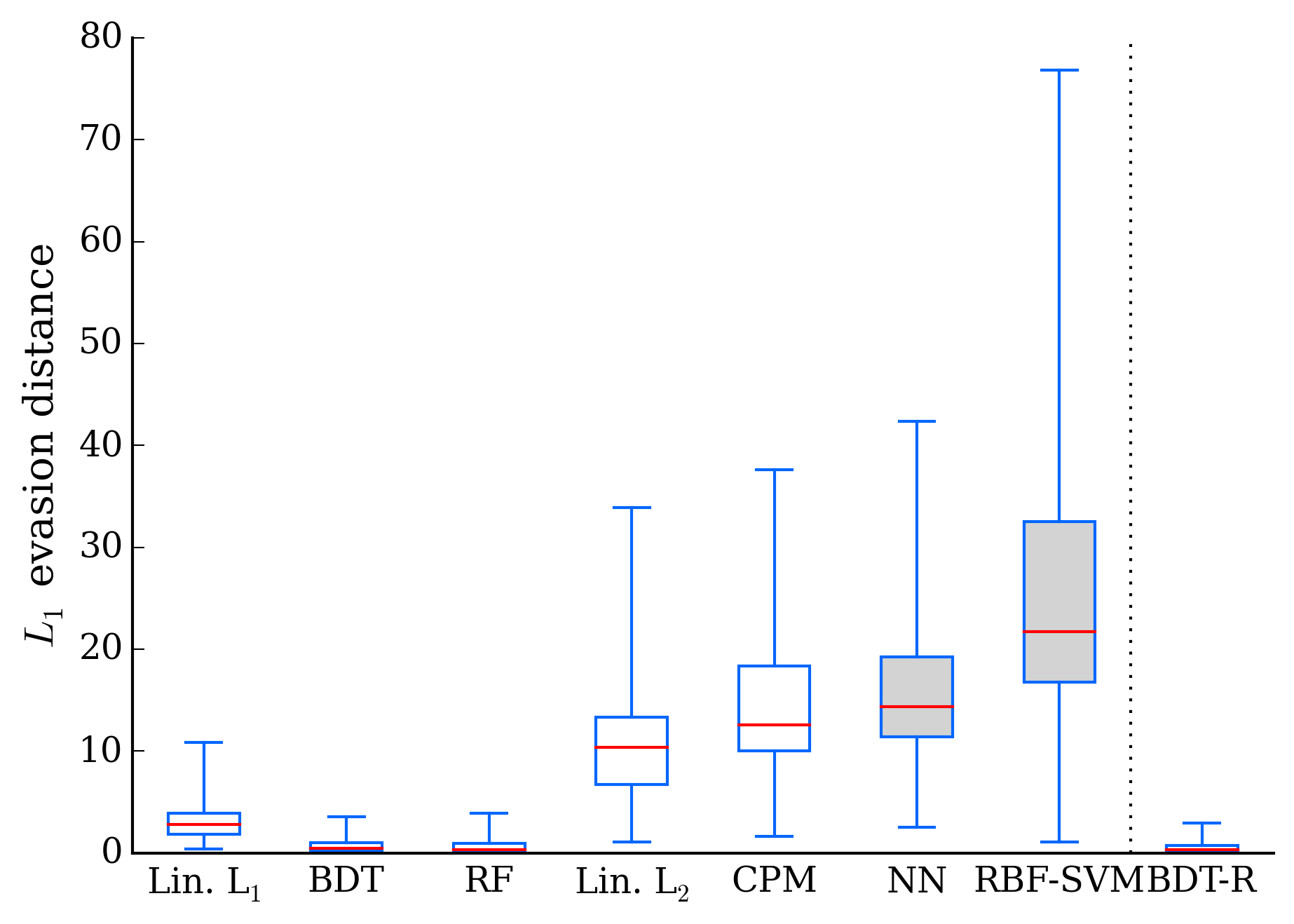
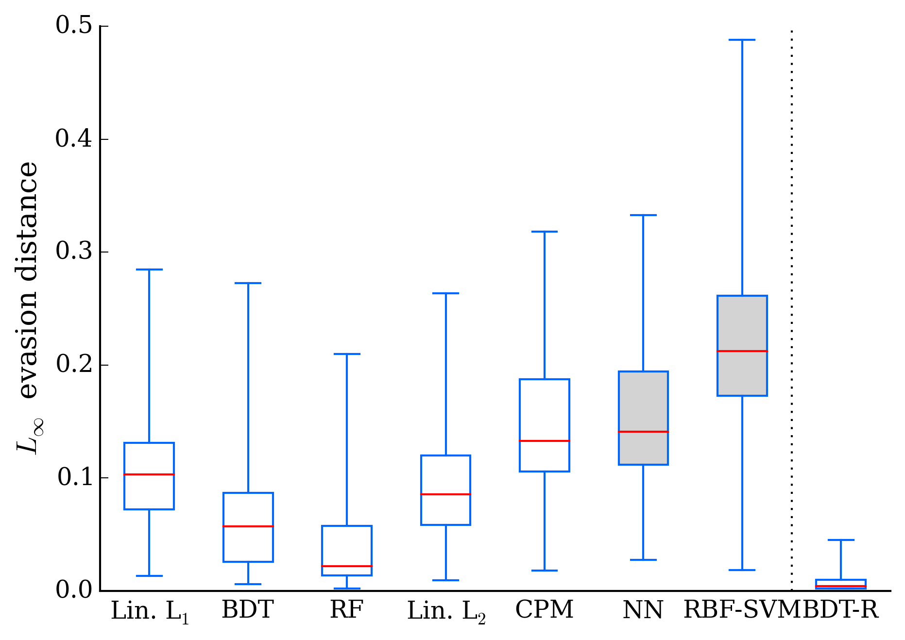
Figure 3: Optimal (white boxes) or best-effort (gray boxes) evasion bounds for different metrics on the evaluation dataset. The smallest bounds, 25-50% and 50-75% quartiles and largest bounds are shown. The red line is the median score. Larger scores mean more deformations are necessary to change the model prediction.

Model	Parameters	Test Error
Lin. $L_{1}$	$C=0.5$	1.5%
Lin. $L_{2}$	$C=0.2$	1.5%
BDT	1,000 trees, depth 4, $\eta=0.02$	0.25%
RF	80 trees, max. depth 22	0.20%
CPM	$k=30$, $C=0.01$	0.20%
NN	60-60-30 sigmoidal (tanh) units	0.25%
RBF-SVM	$\gamma=0.04$, $C=1$	0.25%
BDT-R	1,000 trees, depth 6, $\eta=0.01$	0.20%

Table 1: The considered models. BDT-R is the hardened boosted trees model introduced in section 5.4.

5.1 Dataset and Method

We choose digit recognition over the MNIST (LeCun et al., ) dataset as our benchmark classification task for three reasons. First, the MNIST dataset is well studied and exempt from labeling errors. Second, there is a one-to-one mapping between pixels and features, so that features can vary independently from each other. Third, we can pictorially represent evading instances, and this helps understanding the models’ robustness or lack of. Our running binary classification task is to distinguish between handwritten digits “2” and “6”. Our training and testing sets respectively include 11,876 and 1,990 images and each image has $28\times 28$ gray scale pixels and our feature space is $\mathcal{X}=[0,1]^{784}$. As our main goal is not to compare model accuracies, but rather to obtain the best possible model for each model class, we tune the hyper-parameters so as to minimize the error on the testing set directly. In addition to the training and testing sets, we create an evaluation dataset of a hundred instances from the testing set such that every instance is correctly classified by all of the benchmarked models. These correctly classified instances are to serve the purpose of $x$, the starting point instances in the evasion problem (1).

5.2 Considered Models

Table 1 summarizes the 7 benchmarked models with their salient hyper-parameters and error rates on the testing set. For our tree ensembles, BDT is a (gradient) boosted decision trees model in the modern XGBoost implementation (Chen & He, ) and RF is a random forest trained using scikit-learn (Buitinck et al., 2013). We also include the following models for comparison purposes. Lin. $L_{1}$ and Lin. $L_{2}$ are respectively a $L_{1}$ and $L_{2}$-regularized logistic regression using the LibLinear (Fan et al., 2008) implementation. RBF-SVM is a regular Gaussian kernel SVM trained using LibSVM (Chang & Lin, 2011). NN is a 3 hidden layer neural network with a top logistic regression layer implemented using Theano (Bergstra et al., 2010) (no pre-training, no drop-out). Finally, our last benchmark model is the equivalent of a shallow neural network made of two max-out units (one unit for each class) each made of thirty linear classifiers. This model corresponds to the difference of two Convex Polytope Machines (Kantchelian et al., 2014) (one for each class) and we use the authors’ implementation (CPM). Two factors motivate the choice of CPM. First, previous work has theoretically considered the evasion robustness of such ensemble of linear classifiers and proved the problem to be NP-hard (Stevens & Lowd, 2013). Second, unlike RBF-SVM and NN, this model can be readily reduced to a Mixed Integer Program, enabling optimal evasions thanks to a MIP solver. As the reduction is considerably simpler than the one presented for tree ensembles above, we omit it here. Except for the two linear classifiers, all models have a comparable, very low error rate on the benchmark task.

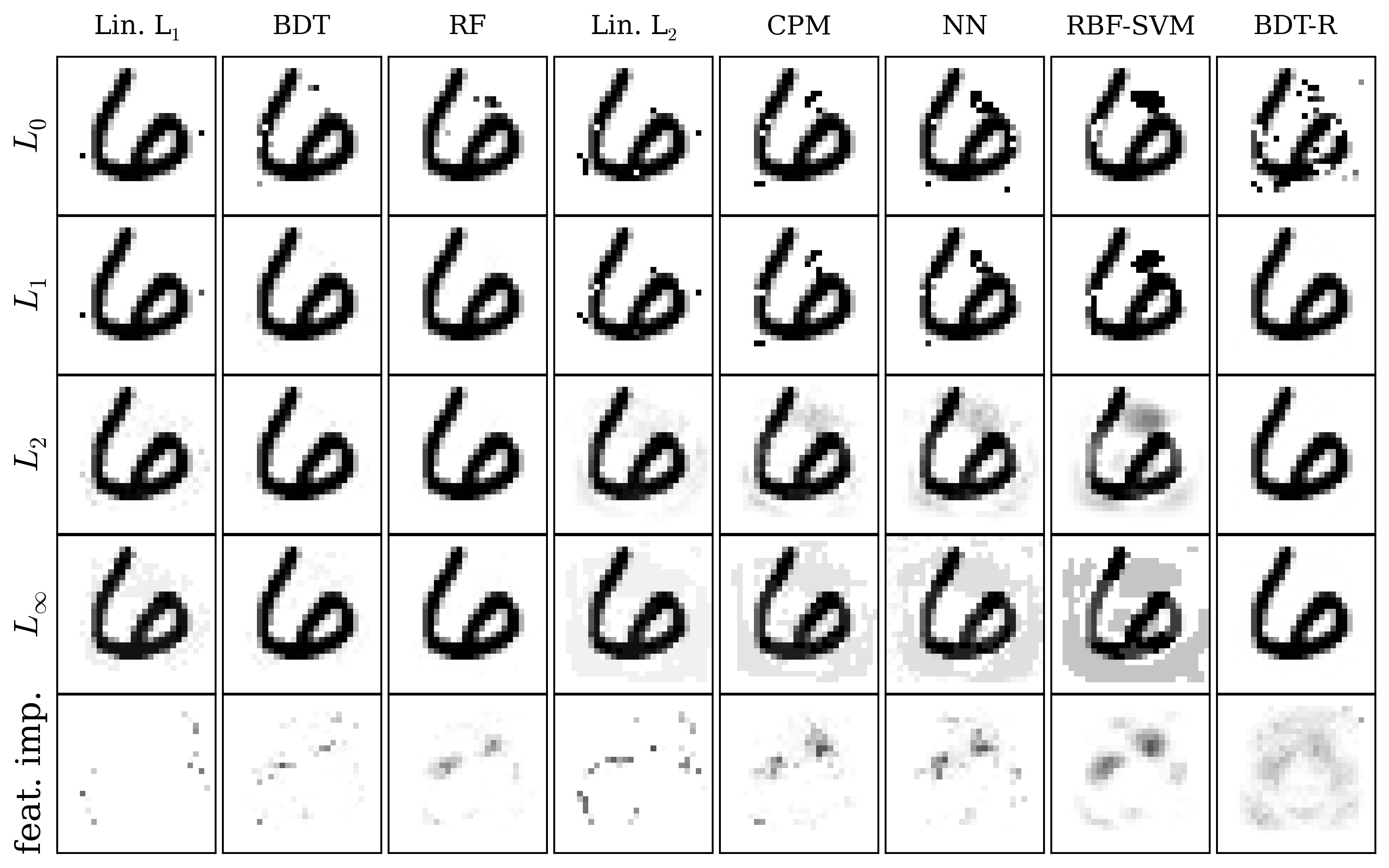
Figure 4: First 4 rows: examples of optimal or best effort evading “6” instances. Every picture is misclassified as “2” by its column model. Last row: feature importance computed as frequency of pixel modification in the $L_{0}$-evasions (darker means feature is more often picked).

5.3 Robustness

For each learned model, and for all of the 100 correctly classified evaluation instance, we compute the optimal (or best effort) solution to the evasion problem under all of the deformation metrics. We use the Gurobi (Gurobi Optimization, 2015) solver to compute the optimal evasions for all distances and all models but NN and RBF-SVM. We use a classic projected gradient descent method for solving the $L_{1},L_{2}$ and $L_{\infty}$ evasions of NN and RBF-SVM, and address the $L_{0}$-evasion case by an iterative coordinate descent algorithm and a brute force grid search at each iteration. Figure 3 summarizes the obtained adversarial bounds as one boxplot for each combination of model and distance. Although the tree ensembles BDT and RF have very competitive accuracies, they systematically rank at the bottom for robustness across all metrics. Remarkably, negligible $L_{1}$ or $L_{2}$ perturbations suffice to evade those models. RBF-SVM is apparently the hardest model to evade, agreeing with results from (Goodfellow et al., 2014). NN and CPM exhibit very similar performance despite having quite different architectures. Finally, the $L_{1}$-regularized linear model exhibits significantly more brittleness than its $L_{2}$ counterpart. This phenomenon is explained by large weights concentrating in specific dimensions as a result of sparsity. Thus, small modifications in the heavily weighted model dimensions can result in large classifier output variations.

5.4 Hardening by Adversarial Boosting

We empirically demonstrate how to significantly improve the robustness of the BDT model by adding evading instances to the training set during the boosting process. At each boosting round, we use our fast symbolic prediction-based algorithm to create budgeted “adversarial” instances with respect to the current model and for all the 11,876 original training instances. For a given training instance $x$ with label $y$ and a modification budget $B\geq 1$, a budgeted “adversarial” training instance $x^{*}$ is such that $\|x-x^{*}\|_{0}\leq B$ and the margin $yf(x^{*})$ is as small as possible. Here, we use $B=28$, the size of the picture diagonal, as our budget. The reason is that modifying 28 pixels over 784 is not enough to perceptually morph a handwritten “2” into “6”. The training dataset for the current round is then formed by appending to the original training dataset these evading instances along with their correct labels, thus increasing the size of the training set by a factor 2. Finally, gradient boosting produces the next regression tree which by definition minimizes the error of the augmented ensemble model on the adversarially-enriched training set. After 1,000 adversarial boosting rounds, our model has encountered more than 11 million adversarial instances, without ever training on more than 24,000 instances at a time.

We found that we needed to increase the maximum tree depth from 4 to 6 in order to obtain an acceptable error rate. After 1,000 iterations, the resulting model BDT-R has a slightly higher testing accuracy than BDT (see Table 1). Unlike BDT, BDT-R is extremely challenging to optimally evade using the MILP solver: the branch-and-bound search continues to expand nodes after 1 day on a 6 core Xeon 3.2GHz machine. To obtain the tightest possible evasion bound, we warm-start the solver with the solution found by the fast evasion technique and report the best solution found by the solver after an hour. Figure 3 shows that BDT-R is more robust than our previous champion RBF-SVM with respect to $L_{0}$ deformations. Unfortunately, we found significantly lower scores on all $L_{1},L_{2}$ and $L_{\infty}$ distances compared to the original BDT model: hardening against $L_{0}$-evasions made the model more sensitive to all other types of evasions.

6 Conclusion

We have presented two novel algorithms, one exact and one approximate, for systematically computing evasions of tree ensembles such as boosted trees and random forests. On a classic digit recognition task, both gradient boosted trees and random forests are extremely susceptible to evasions. We also introduce adversarial boosting and show that it trains models that are hard to evade, without sacrificing accuracy. One future work direction would be to use these algorithms to generate “small” evading instances for practical security systems. Another direction would be to better understand the properties of adversarial boosting. In particular, it is not known whether this hardening approach would succeed on all possible datasets.

References

- Barreno et al. (2006) Barreno, M., Nelson, B., Sears, R., Joseph, A. D., and Tygar, J. D. Can machine learning be secure? In Proceedings of the 2006 ACM Symposium on Information, Computer and Communications Security, ASIACCS ’06, 2006.
- Bergstra et al. (2010) Bergstra, J., Breuleux, O., Bastien, F., Lamblin, P., Pascanu, R., Desjardins, G., Turian, J., Warde-Farley, D., and Bengio, Y. Theano: a CPU and GPU math expression compiler. In Proceedings of the Python for Scientific Computing Conference (SciPy), 2010.
- Biggio et al. (2013) Biggio, B., Corona, I., Maiorca, D., Nelson, B., Šrndić, N., Laskov, P., Giacinto, G., and Roli, F. Evasion attacks against machine learning at test time. In Machine Learning and Knowledge Discovery in Databases, volume 8190 of Lecture Notes in Computer Science. Springer Berlin Heidelberg, 2013.
- Brückner et al. (2012) Brückner, M., Kanzow, C., and Scheffer, T. Static prediction games for adversarial learning problems. The Journal of Machine Learning Research, 13(1):2617–2654, 2012.
- Buitinck et al. (2013) Buitinck, L., Louppe, G., Blondel, M., Pedregosa, F., Mueller, A., Grisel, O., Niculae, V., Prettenhofer, P., Gramfort, A., Grobler, J., Layton, R., VanderPlas, J., Joly, A., Holt, B., and Varoquaux, G. API design for machine learning software: experiences from the scikit-learn project. In ECML PKDD Workshop: Languages for Data Mining and Machine Learning, pp. 108–122, 2013.
- Chang & Lin (2011) Chang, C.C. and Lin, C.J. LIBSVM: A library for support vector machines. ACM Transactions on Intelligent Systems and Technology, 2, 2011.
- (7) Chen, T. and He, T. XGBoost: eXtreme Gradient Boosting. https://github.com/dmlc/xgboost. Accessed: 2015-06-05.
- Dalvi et al. (2004) Dalvi, N., Domingos, P., Mausam, Sanghai, S., and Verma, D. Adversarial classification. In Proceedings of the tenth ACM SIGKDD international conference on Knowledge discovery and data mining, pp. 99–108. ACM, 2004.
- Fan et al. (2008) Fan, R.E., Chang, K.W., Hsieh, C.J., Wang, X.R., and Lin, C.J. LIBLINEAR: A library for large linear classification. Journal of Machine Learning Research, 9, 2008.
- Fawzi et al. (2014) Fawzi, A., Fawzi, O., and Frossard, P. Analysis of classifiers’ robustness to adversarial perturbations. arXiv preprint, 2014.
- Goodfellow et al. (2014) Goodfellow, I. J., Shlens, J., and Szegedy, C. Explaining and harnessing adversarial examples. arXiv preprint, 2014.
- Griva et al. (2008) Griva, I., Nash, S. G., and Sofer, A. Linear and Nonlinear Optimization (2nd edition). Society for Industrial Mathematics, 2008.
- Gu & Rigazio (2015) Gu, S. and Rigazio, L. Towards deep neural network architectures robust to adversarial examples. arXiv preprint, 2015.
- Gurobi Optimization (2015) Gurobi Optimization, Inc. Gurobi optimizer reference manual, 2015. URL http://www.gurobi.com.
- Kantchelian et al. (2014) Kantchelian, A., Tschantz, M. C., Huang, L., Bartlett, P. L., Joseph, A. D., and Tygar, J. D. Large-margin convex polytope machine. In Advances in Neural Information Processing Systems (NIPS), 2014.
- King (1976) King, James C. Symbolic execution and program testing. Communications of the ACM, 19(7):385–394, 1976.
- L. (2005) L., Daniel. Good word attacks on statistical spam filters. In Proceedings of the Second Conference on Email and Anti-Spam (CEAS), 2005.
- (18) LeCun, Yann, Cortes, Corinna, and Burges, Christopher J.C. MNIST dataset, 1998. URL http://yann.lecun.com/exdb/mnist/.
- Lowd & Meek (2005) Lowd, D. and Meek, C. Adversarial learning. In Proceedings of the Eleventh ACM SIGKDD International Conference on Knowledge Discovery in Data Mining, KDD ’05, 2005.
- Nelson et al. (2012) Nelson, B., Rubinstein, B. I. P., Huang, L., Joseph, A. D., Lee, S. J., Rao, S., and Tygar, J. D. Query strategies for evading convex-inducing classifiers. Journal of Machine Learning Research, 13, May 2012.
- Norouzi et al. (2015) Norouzi, M., Collins, M., Johnson, M. A, Fleet, D. J., and Kohli, P. Efficient non-greedy optimization of decision trees. In Advances in Neural Information Processing Systems (NIPS), pp. 1720–1728, 2015.
- Papernot et al. (2015) Papernot, N., McDaniel, P., Wu, X., Jha, S., and Swami, A. Distillation as a defense to adversarial perturbations against deep neural networks. arXiv preprint arXiv:1511.04508, 2015.
- Srndic & Laskov (2014) Srndic, N. and Laskov, P. Practical evasion of a learning-based classifier: A case study. In Proceedings of the 2014 IEEE Symposium on Security and Privacy, S&P ’14, 2014.
- Stevens & Lowd (2013) Stevens, D. and Lowd, D. On the hardness of evading combinations of linear classifiers. In Proceedings of the 2013 ACM Workshop on Artificial Intelligence and Security, AISec ’13, 2013.
- Szegedy et al. (2013) Szegedy, C., Zaremba, W., Sutskever, I., Bruna, J., Erhan, D., Goodfellow, I., and Fergus, R. Intriguing properties of neural networks. arXiv preprint, 2013.
- Xu et al. (2016) Xu, W., Qi, Y., and Evans, D. Automatically evading classifiers: A case study on PDF malware classifiers. In Network and Distributed Systems Security Symposium (NDSS), 2016.