Unraveling the secret of Benjamin Franklin:
Constructing Franklin squares of higher order
Abstract
Benjamin Franklin constructed three squares which have amazing properties, and his method of construction has been a mystery to date. In this article, we divulge his secret and show how to construct such squares for any order.
1 Introduction
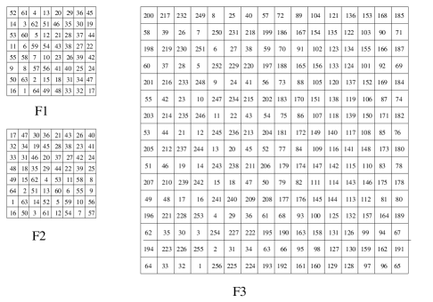
The well-known squares in Figure 1 were constructed by Benjamin Franklin (see [2] and [3]). In a letter to Peter Collinson (see [2]) he describes the properties of the square, F1 as:
-
1.
The entries of every row and column add to a common sum called the magic sum.
-
2.
In every half row and half column the entries add to half the magic sum.
- 3.
-
4.
The four corner numbers with the four middle numbers add to the magic sum.
Franklin mentions that the square F1 has five other curious properties without listing them. He also says, in the same letter, that the square, F3, in Figure 1 has all the properties of the square, but in addition, every sub-square adds to the common magic sum.
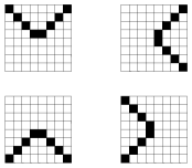
We now bring to attention some important facts about these squares. The entries of the squares are from the set , where or . Every integer in this set occurs in the square exactly once. The squares have magic sum 260 and the square has magic sum 2056. Unlike, F1 or F2, observe that for F3, the four corner numbers with the four middle numbers add to half the magic sum. In addition, observe that every sub-square in F1 and F2 adds to half the magic sum, and in F3 adds to one-quarter the magic sum. The property of the sub-squares adding to a common sum and the property of bend diagonals adding to the magic sum are continuous properties. By continuous property we mean that if we imagine the square is the surface of a torus; i.e. opposite sides of the square are glued together, then the bend diagonals or the sub-squares can be translated and still the corresponding sums hold (see Figure 3). It is worth noticing that the fourth property listed by Benjamin Franklin is redundant because of the continuous property of the sub-squares adding to a common sum. Moreover, the sub-square property implies that every sub-square adds to the magic sum in F3. For a detailed study of these three squares constructed by Benjamin Franklin, see [1, 2, 3].
From now on, row sum, column sum, or bend diagonal sum, etc. mean that we are adding the entries of those elements. We use the description provided by Benjamin Franklin and our observations to define Franklin squares.
Definition 1.1 (Franklin Square).
Consider an integer, such that . Let the magic sum be denoted by and . We define an Franklin square to be a matrix with the following properties:
-
1.
Every integer from the set occurs exactly once in the square. Consequently,
-
2.
All the the half rows, half columns add to one-half the magic sum. Consequently, all the rows and columns add to the magic sum.
-
3.
All the bend diagonals add to the magic sum, continuously.
-
4.
All the sub-squares add to , continuously. Consequently, all the sub-squares add to , and the four corner numbers with the four middle numbers add to .
In [1], we described how to construct Franklin squares using Algebraic Geometry and Combinatorics. Those methods, being computationally challenging, are not suitable for higher orders. In this article, we follow Benjamin Franklin’s footsteps closely, and provide elementary techniques to construct a Franklin square of any given order. The strategies of construction of Franklin squares F1 and F3 are the same and our methods are based on observing these two squares. The construction of F2 is different from F1 and we do not touch upon the construction of F2 in this article. A Franklin square is given in Table 1. A Franklin square of this order has never been constructed before. Moreover, the Maple code we provide in Section 3 can easily construct Franklin squares of higher order. The details of the method are given in in Section 2.
2 Method to construct Franklin squares.
In this section, we describe a process to construct Franklin squares. The squares F1 and F3 can also be constructed with this method.
A Franklin square is constructed in two parts: the left side consisting of the first columns and the right side consisting of the last columns. The construction of both the parts are largely independent of each other. Each side is further divided in to three parts: the top part consisting of the first rows, the middle part consisting of the middle rows, and the bottom part consisting of the last rows. Throughout this article, reference to these parts mean these blocks of rows. Each side is constructed by adding pairs of columns equidistant from its center. For a given part, and a pair of columns, and , there are two operations to make entries, which we call Up and Down. Let denote a part, denote the number of rows in , and let and denote the first and last row of , respectively. Let denote a starting number. Throughout this article, from now on, . The inputs to the functions Up and Down are , , , , , and .
The function Up assigns values to the columns and in the following manner.
For to : and
The function Down assigns values to the square in the manner described below.
For to : and
Observe that the Up function goes up the rows of the part in a zig-zag fashion assigning values and . Similarly, the Down function goes down the rows of the part. Observe that these assignments guarantee that , for any row and pair of columns .
The indices of column pairings and order of construction for the left side is and ; and for the right side is and where . This order of construction implies that the left side is constructed from the center going outwards whereas the right side is constructed from the outside columns going inwards to the center. The numbers always appear on the left side of the Franklin square and the numbers appear on the right side of the square.
We first construct the left side of the Franklin square. To begin, we do an Up operation on the bottom part with , , , and . Then, we do an Up operation on the top part with , , , and . Next, we do a Down operation on the middle part with , , , and . At this point, we have constructed two columns which contain the integers and . Now, we do an Up operation on the middle part with , , , and . Next, we do a Down operation on the top part with , , , and . Finally, we do a Down operation on the bottom part with , , , and .
Observe that four columns were created with the above operations. This sequence of operations is repeated times to complete the left side of the square, where the parameters in the Up and Down operations are replaced by , , , where .
The same sequence of operations and number of repetitions are used to construct the right side of the Franklin square. The parameters and remain the same whereas for all the Up and Down operations. The changes in the column parameters and are listed below.
| Up(bottom) | Up(top) | Down(middle) | Up(middle) | Down(top) | Down(bottom) | |
| ca: | n/2+1 | n/2+1 | n/2+1 | n/2+2 | n/2+2 | n/2+2 |
| cs: | n | n | n | n-1 | n-1 | n-1 |
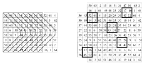
See Figure 4 and Table 2 for a pictorial construction of the left side of the Franklin square F3. The pictorial construction of right side of F3 is described in Figure 5 and Table 3. Maple procedures to construct Franklin squares of any order are provided in Section 3.


Proposition 2.1.
Let be an square constructed by the above procedure. Then is a Franklin square.
Proof.
Consider a column of . Then, for the rows and , if is odd, we have
and if is odd, we have
Consider the remaining rows, that is, . In the top and middle parts of the square, that is, when or , we have
For the middle part of the square, that is, when , we have
Thus, adjacent pair of entries in the column add to within a part of the square. At the boundaries, that is, for the rows and , the sums are slightly different. Nevertheless, because of the alternating signs between odd and even columns, it follows that all the sub-squares add to , continuously.
Also, for the column , the entries of the top four rows and the bottom four rows add to , if is odd, and , if is even. Moreover, the top four rows and the last four rows of the middle part add to , if is odd, and to , if is even. Consequently, all the half columns add to which is half the magic sum. Therefore, all the columns add to the magic sum. Since the rows were constructed by adding paired entries that add to , it follows that all the half rows and rows add to the half the magic and the magic sum, respectively.
Pairs of entries of the column that are equidistant from the center add to the following sums.
If is odd, when (which restricts to the top and bottom parts of ), we have
For the middle part of the square, that is, when , we have
When is even: for the top and bottom part of , which implies, , we have
and for the middle part, where , we get
Consequently, the entries of a right or left diagonal always add to the sum
Hence all the left and right bend diagonals always add to the magic sum.
Along, a top or bottom bend diagonal, two pairs of adjacent diagonal entries equidistant from the center, always, add to as follows.
For and :
Hence all the top diagonals add to the common magic sum, continuously.
For and :
Therefore, all the bottom diagonals add to the common magic sum, continuously.
Thus, we conclude that is a Franklin square.
∎
3 Maple Program to construct Franklin squares.
In this section, we provide a Maple procedure to construct a Franklin square. The input to the procedure is . For example, the command Franklin(16) creates a Franklin square.
# nn is the order of the Franklin square
Franklin := proc(nn)
local A, n, N, i, j,t,s,r,cs,ca,e;
n:=eval(nn);
A := matrix(n,n,0);
N:=n*n+1;
#Start j loop
for j from 0 to n/8-1 do
# Constructing the left half of the square
#Bottom quarter going up
s:=1; r:=n; cs:=n/4; ca:=n/4+1; e:=n/8-1;
Up(A,n,N,s,r,cs, ca,e,j);
#Top quarter going up
s:=n/4+1; r:=n/4; cs:=n/4; ca:=n/4+1; e:=n/8-1;
Up(A,n,N,s,r,cs,ca,e,j);
#Middle half going up
s:=n+1; r:=3*n/4; cs:=n/4-1; ca:=n/4+2; e:=n/4-1;
Up(A,n,N,s,r,cs,ca,e,j);
#Middle half going down
s:=n/2+1; r:=n/4+1; cs:=n/4; ca:=n/4+1; e:=n/4-1;
Down(A,n,N,s,r,cs,ca,e,j);
#Top quarter going down
s:=3*n/2+1; r:=1; cs:=n/4-1; ca:=n/4+2; e:=n/8-1;
Down(A,n,N,s,r,cs,ca,e,j);
#bottom quarter going down
s:=7*n/4+1; r:=3*n/4+1; cs:=n/4-1; ca:=n/4+2; e:=n/8-1;
Down(A,n,N,s,r,cs,ca,e,j);


#Constructing the right half of the square
#Bottom quarter going up
s:=(n/2)*(n/2)+1; r:=n; ca:=n/2+1; cs:=n; e:=n/8-1;
Up(A,n,N,s,r,cs,ca,e,j);
#Top quarter going up
s:=(n/2)*(n/2)+n/4+1; r:=n/4; ca:=n/2+1; cs:=n; e:=n/8-1;
Up(A,n,N,s,r,cs,ca,e,j);
#Middle half going up
s:=(n/2)*(n/2)+n+1; r:=3*n/4; ca:=n/2+2; cs:=n-1; e:=n/4-1;
Up(A,n,N,s,r,cs,ca,e,j);
#Middle half going down
s:=(n/2)*(n/2)+n/2+1; r:=n/4+1; ca:=n/2+1; cs:=n; e:=n/4-1;
Down(A,n,N,s,r,cs,ca,e,j);
#Top quarter going down
s:=(n/2)*(n/2)+3*n/2+1; r:=1; ca:=n/2+2; cs:=n-1; e:=n/8-1;
Down(A,n,N,s,r,cs,ca,e,j);
#bottom quarter going down
s:=(n/2)*(n/2)+7*n/4+1; r:=3*n/4+1; ca:=n/2+2; cs:=n-1; e:=n/8-1;
Down(A,n,N,s,r,cs,ca,e,j);
od; # end of j loop
print(A);
end;

# The Procedures Up and Down that are called from the Franklin main procedure

Up := proc(A,n,N,s,r,cs,ca,e,j)
local i,t;
for i from 0 to e do
t:=s+2*j*n+2*i;
A[r-2*i,cs-2*j] := t;
A[r-2*i,ca+2*j]:= N-t;
A[r-1-2*i,cs-2*j] := N-(t+1);
A[r-1-2*i,ca+2*j]:= t+1;
od;
end;

Down := proc(A,n,N,s,r,cs,ca,e,j)
local i,t;
for i from 0 to e do
t:=s+2*j*n+2*i;
A[r+2*i,cs-2*j] := N-t;
A[r+2*i,ca+2*j]:= t;
A[r+1+2*i,cs-2*j] := t+1;
A[r+1+2*i,ca+2*j]:= N-(t+1);
od;
end;
References
- [1] Ahmed, M., How many squares are there, Mr. Franklin?: Constructing and Enumerating Franklin Squares, Amer. Math. Monthly, Vol. 111, 2004, 394–410.
- [2] Andrews, W. S., Magic Squares and Cubes, 2nd. ed., Dover, New York, 1960.
- [3] Pasles, P. C., The lost squares of Dr. Franklin: Ben Franklin’s missing squares and the secret of the magic circle, Amer. Math. Monthly, 108, (2001), 489-511.