A dedicated greedy pursuit algorithm
for sparse spectral representation of music sound

Abstract

A dedicated algorithm for sparse spectral representation of music sound is presented. The goal is to enable the representation of a piece of music signal as a linear superposition of as few spectral components as possible, without affecting the quality of the reproduction. A representation of this nature is said to be sparse. In the present context sparsity is accomplished by greedy selection of the spectral components, from an overcomplete set called a dictionary. The proposed algorithm is tailored to be applied with trigonometric dictionaries. Its distinctive feature being that it avoids the need for the actual construction of the whole dictionary, by implementing the required operations via the Fast Fourier Transform. The achieved sparsity is theoretically equivalent to that rendered by the Orthogonal Matching Pursuit method. The contribution of the proposed dedicated implementation is to extend the applicability of the standard Orthogonal Matching Pursuit algorithm, by reducing its storage and computational demands. The suitability of the approach for producing sparse spectral representation is illustrated by comparison with the traditional method, in the line of the Short Time Fourier Transform, involving only the corresponding orthonormal trigonometric basis.

Keywords:  Sparse Representation of Music Signals; Self Projected Matching Pursuit.

PACS: 43.75.Zz, 43.60

I Introduction

Spectral representation is a classical approach which plays a central role in the analysis and modelling of both, music sounds (Serra and Smith, 1990; Fletcher and Rossing, 1998; Davy and Godsill, 2003) and acoustic properties of music instruments (Wolfe et al., 2001).

Available techniques aiding the spectral analysis of music range from the Fast Fourier Transform (FFT) and Short Time Fourier Transform (STFT) to several classes of joint Time Frequency$/$Scale distributions (Alm and Walker, 2002; Smith 2011) and atomic representations (Mallat and Zhang, 1993; Gribonval and Bacry, 2003).

In this Communication we focus on the representation of a digital piece of music, as the superposition of vectors arising by the discretization of trigonometric functions. The aim is to represent segments of a sound signal, as a linear combination of as few spectral components as possible without affecting the quality of the sound reproduction. We referrer to the sought representation as piecewise sparse spectral representation of music sound. Additionally to the typical advantages of sparse signal representation, the emerging theory of compressive$/$compressed sensing (Baraniuk, 2007, 2011; Donoho, 2006; Candès, et al. 2006; Candès and Wakin, 2008) has introduced a renewed strong reason to pursue sparse representation of music. This theory associates sparsity to a new framework for digitalization, beyond the Nyquist$/$Shannon sampling theorem. Within the compressive sensing framework, the number of measurements needed for accurate representation of a signal informational content decreases, if the sparsity of the representation improves.

For the class of compressible signals the sparse approximation can be accomplished by representation in an orthonormal basis, simply by disregarding the least significant terms in the decomposition. Melodic music signals are known to be compressible in terms of trigonometric orthonormal basis. However, a much higher level of sparsity may be achieved by releasing the orthogonality property of the spectral components (Mallat and Zhang, 1993; Gribonval and Bacry, 2003; Rebollo-Neira, 2016a). The price to be paid for that is the increment in the complexity of the numerical algorithms producing the corresponding sparser approximation. Practical algorithms for this purpose are known as greedy pursuit strategies (Friedman and Stuetzle, 1981; Jones, 1987; Mallat and Zhang, 1993). In Gribonval and Bacry (2003) a dedicated Matching Pursuit method for effective implementation of the spectral model is developed by means of well localized frequency components of variable length. In Rebollo-Neira (2016a) an alternative approach is considered. It involves the approximation of a signal by partitioning, according to the following steps: i)The signal is divided into small units (blocks) ii)Each block is approximated by nonorthogonal spectral components, independently of each other but somewhat ‘linked’ by a global constraint on sparsity or quality. The global constraint is fulfilled by establishing a hierarchy for the order in which each element in the partition is to be approximated. Thus, the method requires significant storage. Even if the global constraint is disregarded, and each unit approximated totally independent of the others, the algorithms in Rebollo-Neira (2016a) are effective for partition units of moderate length. For units of larger size there is a need of mathematics algorithms specialized to that situation. This is the goal of the present work. We propose a dedicated algorithm for nonorthogonal sparse spectral modeling which, as a consequence of allowing for relatively large elements in a partition, somewhat reduces the need for a global constraint on sparsity. This makes it possible for the approximation of each unit up to the same quality and completely independent of the others. The approach is, thereby, suitable for straightforward parallelization in multiprocessors. As far as sparsity is concerned, the results are theoretical equivalents to those produced by the effective Orthogonal Matching Pursuit method (Pati et al., 1993). The particularity of the proposed implementation, dedicated to trigonometric dictionaries, is that it avoids the need for storing the whole dictionary and reduces the complexity of calculations via the Fast Fourier Transform. The relevance of sparse spectral representation with trigonometric dictionaries, in the context of music compression with high quality recovery, is illustrated in Rebollo-Neira (2016b).

The paper is organized as follows: Sec. II discusses the spectral model outside the traditional orthogonal framework. The mathematical methods for operating within the nonorthogonal setting are also discussed in this section, motivating the proposed dedicated approach. The approach is first explained and then summarized in the form of pseudocodes (Algorithms 1-6) given in Appendix A. The examples of Sec. III illustrate the benefit of a nonorthogonal framework, against the orthogonal one, in relation to the very significant gain in the sparsity of the spectral representation of music signals for high quality recovery. The results presented in this section demonstrate the relevance of the proposed greedy strategy dedicated to be applied with trigonometric dictionaries. The conclusions are summarized in Sec. IV.

II Sparse Spectral Representation

Let’s assume that a sound signal is given by $N$ sample values, $f(j),\,j=1,\ldots,N$, which are modeled by the following transformation:

$$f(j)=\frac{1}{\sqrt{N}}\sum_{n=1}^{M}c(n)e^{\imath\frac{2\pi(j-1)(n-1)}{M}},\quad j=1,\ldots,N.$$ (1)

For $M=N$ the set of vectors $\{\frac{1}{\sqrt{N}}e^{\imath\frac{2\pi(j-1)(n-1)}{M}},\,j=1,\ldots,N\}_{n=1}^{M}$ is an orthonormal basis for the subspace of $N$-dimensional vectors of complex components. Thus the coefficients in (1) are easily obtained as

$$c(n)=\frac{1}{\sqrt{N}}\sum_{j=1}^{M}f(j)e^{-\imath\frac{2\pi(j-1)(n-1)}{M}},\quad n=1,\ldots,M=N.$$ (2)

Equations (1) and (2) can be evaluated in a fast manner via the FFT.

Suppose now that $M>N$. In that case the set $\{\frac{1}{\sqrt{N}}e^{\imath\frac{2\pi(j-1)(n-1)}{M}},\,j=1,\ldots,N\}_{n=1}^{M}$ is no longer an orthonormal basis but a tight frame (Young, 1980, Daubechies, 1992). From a computational viewpoint the difference with the case $M=N$ is much less pronounced than the theoretical difference. Certainly, when dealing with a tight frame the coefficients in (1) can still be calculated via FFT, by zero padding. The differences though with the orthogonal case are major.

• When $M>N$ the coefficients in the superposition (1) are not unique. The addition of a linear combination with coefficients taken as the components of any vector in the null space of the transformation would not affect the reconstruction.

• The tight frame coefficients calculated via FFT, by zero padding, produce the unique coefficients minimizing the square norm $\displaystyle{{\sum_{n=1}^{M}|c(n)|^{2}}}$. Such a solution is not sparse.

• For the case $M=N$ the approximation obtained through (1), by disregarding coefficients of small magnitude, is optimal in the sense of minimizing the norm of the residual error. This is not true when $M>N$, in which case the nonzero coefficients need to be re-calculated to attain the equivalent optimality (Rebollo-Neira, 2007).

In order to construct an optimal approximation of the data by a representation of the form (1), with $M>N$ but containing at most $k$ non zero coefficients, those coefficients have to be appropriately calculated. Let’s suppose that we want to involve only the elements $\ell_{n},\,n=1,\ldots,k$ where each $\ell_{n}$ is a different member from the set $\{1,2,\cdots,M\}$. Then the approximation model takes the form

$$f^{k}(j)=\frac{1}{\sqrt{N}}\sum_{n=1}^{k}c^{k}(\ell_{n})e^{\imath\frac{2\pi(j-1)(\ell_{n}-1)}{M}},\quad j=1,\ldots,N.$$ (3)

The superscript $k$ in the coefficients $c^{k}(\ell_{n}),\,n=1,\ldots,k$ indicates that they have to be recalculated if some terms are added to (or eliminated from) the model (3). We address the matter of choosing the $k$ elements in (3) by a dedicated Self Projected Matching Pursuit (SPMP) approach (Rebollo-Neira and Bowley, 2013).

A Self Projected Matching Pursuit

Before reviewing the general SPMP technique let’s define some basic notation: $\mathbb{R},\mathbb{C}$ and $\mathbb{N}$ represent the sets of real, complex and natural numbers, respectively. Boldface letters are used to indicate Euclidean vectors and standard mathematical fonts for their components, e.g., $\mathbf{d}\in\mathbb{C}^{N}$ is a vector of $N$-components $d(j)\in\mathbb{C}^{N}\,,j=1,\ldots,N$. The operation $\langle\cdot,\cdot\rangle$ indicates the Euclidean inner product and $\|\cdot\|$ the induced norm, i.e. $\|\mathbf{d}\|^{2}=\langle\mathbf{d},\mathbf{d}\rangle$, with the usual inner product definition: For $\mathbf{d}\in\mathbb{C}^{N}$ and $\mathbf{f}\in\mathbb{C}^{N}$

$$\langle\mathbf{f},\mathbf{d}\rangle=\sum_{j=1}^{N}f^{\ast}(j)d(j),$$

where $f^{\ast}(j)$ stands for the complex conjugate of $f(j)$.

Let’s consider now a set $\mathcal{D}$ of $M$ normalized to unity vectors $\mathcal{D}=\{\mathbf{d}_{n}\in\mathbb{C}^{N}\,;\|\mathbf{d}_{n}\|=1\}_{n=1}^{M}$ spanning $\mathbb{C}^{N}$. For $M>N$ the over-complete set $\mathcal{D}$ is called a dictionary and the elements are called atoms. Given a signal, as a vector $\mathbf{f}\in\mathbb{C}^{N}$, the $k$-term atomic decomposition for its approximation takes the form

$$\mathbf{f}^{k}=\sum_{n=1}^{k}c^{k}(\ell_{n})\mathbf{d}_{\ell_{n}}.$$ (4)

The problem of how to select from $\mathcal{D}$ the $k$ elements $\mathbf{d}_{\ell_{n}},\,n=1\ldots,k$, such that $\|\mathbf{f}^{k}-\mathbf{f}\|$ is minimal, is an NP-hard problem (Natarajan, 1995). The equivalent problem, that of finding the sparsest representation for a given upper bound error, is also NP hard. Hence, in practical applications one looks for ‘tractable sparse’ solutions. This is a representation involving a number of $k$-terms, with $k$ acceptable small in relation to $N$. Effective techniques available for the purpose are in the line of Matching Pursuit Strategies. The seminal approach, Matching Pursuit (MP), was introduced with this name in the context of signal processing by Mallat and Zhang (1993). Nevertheless, it had appeared previously as a regression technique in statistics (Friedman and Stuetzle, 1981) where the convergence property was established (Jones, 1987). The MP implementation is very simple. It evolves by successive approximations as follows.

Let $\mathbf{R}^{k}$ be the $k$-th order residue defined as $\mathbf{R}^{k}=\mathbf{f}-\mathbf{f}^{k}$, and $\ell_{k+1}$ the index for which the corresponding dictionary atom $\mathbf{d}_{\ell_{k+1}}$ yields a maximal value of $|\langle\mathbf{d}_{n},\mathbf{R}^{k}\rangle|,\,n=1,\ldots M$. Starting with an initial approximation $\mathbf{f}^{0}=0$ and $\mathbf{R}^{0}=\mathbf{f}-\mathbf{f}^{0}$ the algorithm iterates by sub-decomposing the $k$-th order residue into

$$\mathbf{R}^{k}=\langle\mathbf{d}_{\ell_{k+1}},\mathbf{R}^{k}\rangle\mathbf{d}_{\ell_{k+1}}+\mathbf{R}^{k+1},$$ (5)

which defines the residue at order $k+1$. Because the atoms are normalized to unity $\mathbf{R}^{k+1}$ given in (5) is orthogonal to $\mathbf{d}_{\ell_{k+1}}$. Hence it is true that

$$\|\mathbf{R}^{k}\|^{2}=|\langle\mathbf{d}_{\ell_{k+1}},\mathbf{R}^{k}\rangle|^{2}+\|\mathbf{R}^{k+1}\|^{2},\quad n=1,\ldots,M,$$ (6)

from where one gathers that the dictionary atom $\mathbf{d}_{\ell_{k+1}}$ yielding a maximal value of $|\langle\mathbf{R}^{k},\mathbf{d}_{n}\rangle|$ minimizes $\|\mathbf{R}^{k+1}\|^{2}$. Moreover, it follows from (5) that at iteration $k$ the MP algorithm results in an intermediate representation of the form:

$$\mathbf{f}=\mathbf{f}^{k}+\mathbf{R}^{k+1},$$ (7)

with

$$\mathbf{f}^{k}=\sum_{n=1}^{k}\langle\mathbf{d}_{\ell_{n}},\mathbf{R}^{n-1}\rangle\mathbf{d}_{\ell_{n}}.$$ (8)

In the limit $k\rightarrow\infty$ the sequence $\mathbf{f}^{k}$ converges to $\mathbf{f}$, or to $\hat{P}_{\mathbb{V}_{M}}\mathbf{f}$, the orthogonal projection of $\mathbf{f}$ onto $\mathbb{V}_{M}={\mbox{\rm{span}}}\{\mathbf{d}_{\ell_{n}}\}_{n=1}^{M}$ if $\mathbf{f}$ were not in $\mathbb{V}_{M}$ (Jones, 1987; Mallat and Zhang, 1993; Partington 1997). Nevertheless, if the algorithm is stopped at the $k$th-iteration, $\mathbf{f}^{k}$ recovers an approximation of $\mathbf{f}$ with an error equal to the norm of the residual $\mathbf{R}^{k+1}$ which, if the selected atoms are not orthogonal, will not be orthogonal to the subspace they span. An additional drawback of the MP approach is that the selected atoms may not be linearly independent. As illustrated in Rebollo-Neira and Bowley (2013), this drawback may significantly compromise sparsity in some cases. A refinement to MP, which does yield an orthogonal projection approximation at each step, has been termed Orthogonal Matching Pursuit (OMP) (Pati et al., 1993). In addition to selecting only linearly independent atoms, the OMP approach improves upon MP numerical convergence rate and therefore amounts to be, usually, a better approximation of a signal after a finite number of iterations. OMP provides a decomposition of the signal of the form:

$$\mathbf{f}=\sum_{n=1}^{k}c^{k}(\ell_{n})\mathbf{d}_{\ell_{n}}+\tilde{\mathbf{R}}^{k},$$ (9)

where the coefficients $c^{k}(\ell_{n})$ are computed to guarantee that

$$\sum_{n=1}^{k}c^{k}(\ell_{n})\mathbf{d}_{\ell_{n}}=\hat{P}_{\mathbb{V}_{k}}\mathbf{f},\quad{\text{with}}\quad\mathbb{V}_{k}={\mbox{\rm{span}}}\{\mathbf{d}_{\ell_{n}}\}_{n=1}^{k}.$$ (10)

The coefficients giving rise to the orthogonal projection $\hat{P}_{\mathbb{V}_{k}}\mathbf{f}$ can be calculated as $c^{k}(\ell_{n})=\langle\mathbf{b}_{n}^{k},\mathbf{f}\rangle$, where the vectors $\mathbf{b}_{n}^{k},\,n=1,\ldots,k$ are biorthogonal to the selected atoms $\mathbf{d}_{\ell_{n}},\,,n=1,\ldots,k$ and span the identical subspace, i.e., ${\displaystyle{\mathbb{V}_{k}={\mbox{\rm{span}}}\{\mathbf{b}_{n}^{k}\}_{n=1}^{k}={\mbox{\rm{span}}}\{\mathbf{d}_{\ell_{n}}\}_{n=1}^{k}}}$. These coefficients yield the unique element $\mathbf{f}^{k}\in\mathbb{V}_{k}$ minimizing $\|\mathbf{f}^{k}-\mathbf{f}\|$. A further optimization of MP, called Optimized Orthogonal Matching Pursuit (OOMP) improves on OMP by also selecting the atoms yielding stepwise minimization of $\|\mathbf{f}^{k}-\mathbf{f}\|$ (Rebollo-Neira and Lowe, 2002). Both OMP and OOMP are very effective approaches for processing signals up to some dimensionality. They become inapplicable, due to its storage requirements, when the signal dimension exceeds some value. Since large signals are approximated by partitioning, up to some size of the partition unit both OMP and OOMP are suitable tools. For considering units of size exceeding the limit of OMP applicability, the alternative implementation, SPMP, which yields equivalent results (Rebollo-Neira and Bowley, 2013) is to be applied. The latter is based on the fact that, as already mentioned, the seminal MP approach converges asymptotically to the orthogonal projection onto the span of the selected atoms. Hence MP itself can be used to produce an orthogonal projection of the data, at each iteration, by self-projections. The orthogonal projection is realized by subtracting from the residue its approximation constructed through the MP approach, but only using the already selected atoms as dictionary. This avoids the need of computing and storing the above introduced vectors $\mathbf{b}_{n}^{k},\,n=1,\ldots,k$, for calculating the coefficients in (10).

The SPMP method progresses as follows (Rebollo-Neira and Bowler, 2013). Given a dictionary $\mathcal{D}=\{\mathbf{d}_{n}\in\mathbb{C}^{N}\,;\|\mathbf{d}_{n}\|=1\}_{n=1}^{M}$ and a signal $\mathbf{f}\in\mathbb{C}^{N}$, set $S_{0}=\{\emptyset\}$, $\mathbf{f}^{0}=0$, and $\mathbf{R}^{0}=\mathbf{f}$. Starting with $k=1$, at each iteration $k$ implement the steps below.

• Apply the MP criterion described above for selecting one atom from $\mathcal{D}$, i.e., select $\ell_{k}$ such that

  $$\ell_{k}=\operatorname*{arg\,max}_{\begin{subarray}{c}n=1,\ldots,M\end{subarray}}|\langle\mathbf{d}_{n},\mathbf{R}^{k-1}\rangle|$$ (11)

  and assign $S_{k}=S_{k-1}\cup\mathbf{d}_{\ell_{k}}$. Update the approximation of $\mathbf{f}$ as $\mathbf{f}^{k}=\mathbf{f}^{k-1}+\langle\mathbf{d}_{\ell_{k}},\mathbf{R}^{k-1}\rangle\mathbf{d}_{\ell_{k}}$ and evaluate the new residue $\mathbf{R}^{k}=\mathbf{f}-\mathbf{f}^{k}$.

• Approximate $\mathbf{R}^{k}$ using only the selected set $S_{k}$ as the dictionary, which guarantees the asymptotic convergence to the approximation $\hat{P}_{\mathbb{V}_{k}}{\mathbf{R}^{k}}$ of $\mathbf{R}^{k}$, where $\mathbb{V}_{k}={\mbox{\rm{span}}}\{S_{k}\}$, and a residue $\mathbf{R}^{\perp}={\mathbf{R}^{k}}-\hat{P}_{\mathbb{V}_{k}}\mathbf{R}^{k}$ having no component in $\mathbb{V}_{k}$.

• Set $\mathbf{f}^{k}\leftarrow\mathbf{f}^{k}+\hat{P}_{\mathbb{V}_{k}}\mathbf{R}^{k},\mathbf{R}^{k}\leftarrow\mathbf{R}^{\perp},k\leftarrow k+1$, and repeat steps i) - iii) until, for a required $\rho$, the condition $\|\mathbf{R}^{k}\|<\rho$ is reached.

B Dedicated SPMP algorithm for sparse spectral decomposition

Even if SPMP reduces the storage requirements for calculating and adapting the coefficients of an atomic decomposition, storage and complexity remains an issue for processing a signal by partitioning in units of considerable size. Notice that the SPMP method involves repetitive calculations of inner products. The advantage of using a trigonometric dictionary, in addition to rendering highly sparse representations in relation to a trigonometric basis, is that a trigonometric dictionary allows the design of a dedicate SPMP implementation, which avoids the construction and storage of the actual dictionary by calculating inner products via FFT.

From now on we shall make use of the knowledge that a piece of music is given by real numbers, i.e. $\mathbf{f}\in\mathbb{R}^{N}$. The dictionaries we consider for producing sparse spectral decompositions of the data are: the Redundant Discrete Fourier (RDF) dictionary, $\mathcal{D}^{f}$, the Redundant Discrete Cosine (RDC) dictionary, $\mathcal{D}^{c}$, and the Redundant Discrete Sine (RDS) dictionary, $\mathcal{D}^{s},$ defined below.

• $\mathcal{D}^{f}=\{\frac{1}{\sqrt{N}}\,e^{\imath\frac{{2\pi(j-1)(n-1)}}{M}},\,j=1,\ldots,N\}_{n=1}^{M}.$

• $\mathcal{D}^{c}=\{\frac{1}{w^{c}(n)}\,\cos({\frac{{\pi(2j-1)(n-1)}}{2M}}),\,j=1,\ldots,N\}_{n=1}^{M}.$

• $\mathcal{D}^{s}=\{\frac{1}{w^{s}(n)}\,\sin({\frac{{\pi(2j-1)n}}{2M}}),\,j=1,\ldots,N\}_{n=1}^{M},$

where $w^{c}(n)$ and $w^{s}(n),\,n=1,\ldots,M$ are normalization factors as given by

$$w^{c}(n)=\begin{cases}\sqrt{N}&\mbox{if}\quad n=1,\\ \sqrt{\frac{N}{2}+\frac{\sin(\frac{\pi(n-1)}{M})\sin(\frac{2\pi(n-1)N}{M})}{2(1-\cos(\frac{2\pi(n-1)}{M}))}}&\mbox{if}\quad n\neq 1.\end{cases}$$

$$w^{s}(n)=\begin{cases}\sqrt{N}&\mbox{if}\quad n=1,\\ \sqrt{\frac{N}{2}-\frac{\sin(\frac{\pi n}{M})\sin(\frac{2\pi nN}{M})}{2(1-\cos(\frac{2\pi n}{M}))}}&\mbox{if}\quad n\neq 1.\end{cases}$$

For $M=N$ each of the above dictionaries is an orthonormal basis, the Orthogonal Discrete Fourier (ODF), Cosine (ODC), and Sine (ODS) basis, henceforth to be denoted as $\mathcal{B}^{f}$ $\mathcal{B}^{c}$ and $\mathcal{B}^{s}$ respectively. The joint mixed dictionary $\mathcal{D}^{cs}=\mathcal{D}^{c}\cup\mathcal{D}^{s}$, with $\mathcal{D}^{c}$ and $\mathcal{D}^{s}$ having the same number of elements, is an orthonormal basis for $M=\frac{N}{2}$, the Orthogonal Discrete Cosine-Sine (ODCS) basis to be indicated as $\mathcal{B}^{cs}$. If $M>\frac{N}{2}$, $\mathcal{D}^{cs}$ becomes a Redundant Discrete Cosine and Sine (RDCS) dictionary.

For facilitating the discussion of fast calculation of inner products with trigonometric atoms, given a vector $\mathbf{y}\in\mathbb{C}^{N}$, let’s define

$${\cal{F}}(\mathbf{y},n,M)=\sum_{j=1}^{N}y(j)e^{-\operatorname{\imath}2\pi\frac{(n-1)(j-1)}{M}},\quad n=1,\ldots,M.$$ (12)

When $M=N$ (12) is the Discrete Fourier Transform of vector $\mathbf{y}\in\mathbb{C}^{N}$, which can be evaluated using FFT. If $M>N$ we can still calculate (12) via FFT by padding with $(M-N)$ zeros the vector $\mathbf{y}$. Equation (12) can also be used to calculate inner products with the atoms in dictionaries $\mathcal{D}^{c}$ and $\mathcal{D}^{s}$. Indeed,

$$\sum_{j=1}^{N}\cos{\frac{{\pi(2j-1)(n-1)}}{2M}}y(j)=\operatorname{Re}\left(e^{-\operatorname{\imath}\frac{\pi(n-1)}{2M}}{\cal{F}}(\mathbf{y},n,2M)\right),\,n=1,\ldots,M.$$ (13)

and

$$\sum_{j=1}^{N}\sin{\frac{{\pi(2j-1)(n-1)}}{2M}}y(j)=-\operatorname{Im}\left(e^{-\operatorname{\imath}\frac{\pi(n-1)}{2M}}{\cal{F}}(\mathbf{y},n,2M)\right),\,n=2,\ldots,M+1,$$ (14)

where $\operatorname{Re}(z)$ indicates the real part of $z$, $\operatorname{Im}(z)$ its imaginary part, and the notation ${\cal{F}}(\mathbf{y},n,2M)$ implies that the vector $\mathbf{y}$ is padded with $(2M-N)$ zeros.

We associate the dictionaries $\mathcal{D}^{f},\mathcal{D}^{c},\mathcal{D}^{s}$ and $\mathcal{D}^{cs}$ to the cases I, II, III, and IV, of the dedicated SPMP Algorithm (SPMPTrgFFT), which is developed in Algorithm 6 of Appendix A, by recourse to the procedures given in Algorithms 1-5.

C Procedures for an implementation of the SPMP method dedicated to trigonometric dictionaries

Let us recall once again that the aim of the present work is to be able to apply the SPMP algorithm, witch is theoretically equivalent to the OMP method, but without evaluating and storing the dictionaries $\mathcal{D}^{f},\mathcal{D}^{c},\mathcal{D}^{s}$ or $\mathcal{D}^{cs}$. Instead, only the selected atoms are evaluated (Algorithm 2) and the inner products are performed via FFT (Algorithm 1). Apart from that, the dedicated implementation follows the steps of the general SPMP method. Some particular features are worth remarking.

• Notice that for Case I, as a consequence of the data being real numbers, it holds that ${\cal{F}}(\mathbf{y},n,M)={\cal{F}}^{\ast}(\mathbf{y},M-n+2,M)$. Hence the atoms can be taken always in pairs, $\ell_{k}$ and $(M-\ell_{k}+2)$.

• The procedure for self projection of MP (Algorithm 5), is a recursive implementation of the selection procedure, but the selection is carried out only over the, say $k$, already selected atoms (Algorithm 4). Then the calculation of the relevant inner products is worth being carried out via FFT only for values of $k$ larger than ${\displaystyle{\frac{M}{N}\log_{2}M}}$.

• In order to provide all the implementation details of the proposed method in a clear and testable manner, we have made publicly available a MATLAB version of the pseudocodes (Algorithms 1-6), as well as the script and the signals which will allow the interested researcher to reproduce the numerical results in this paper . The MATLAB routines should be taken only as ‘demonstration material’. They are not intended to be an optimized implementation of the algorithms. Such optimization should depend on the programming language used for practical applications.

III Numerical Examples

We apply now the SPMPTrgFFT algorithm to produce a sparse spectral representation of the sound clips listed in Table 1 and Table 2. The approximation is carried out by dividing the signals into disjoint pieces $\mathbf{f}_{q}\in\mathbb{R}^{N_{b}},\,q=1,\ldots,Q$ of uniform length $N_{b}$, i.e., $\mathbf{f}=\hat{J}_{q=1}^{Q}\mathbf{f}_{q}$, where $\hat{J}$ indicates a concatenation operation and $N=QN_{b}$.

The purpose of the numerical example is to illustrate the relevance of the method to produce sparse spectral representation of music, in comparison to the classical orthogonal representation in the line of STFT. Each segment $q$ is approximated up to the same quality. The sparsity is measured by the Sparsity Ratio (SR) defined as $\displaystyle{\text{SR}=\frac{N}{K}}$, where $K$ is the total number of coefficients in the signal representation, i.e, denoting by $k_{q}$ the number of coefficients for approximating the $q$-th segment $K=\sum_{q=1}^{Q}k_{q}$.

As a measure of approximation quality we use the standard Signal to Noise Ratio (SNR),

$$\text{SNR}=10\log_{10}\frac{\|\mathbf{f}\|^{2}}{\|\mathbf{f}-\mathbf{f}^{k}\|^{2}}=10\log_{10}\frac{\sum_{\begin{subarray}{c}j=1\\ q=1\end{subarray}}^{N_{b},Q}|f_{q}(j)|^{2}}{\sum_{\begin{subarray}{c}j=1\\ q=1\end{subarray}}^{N_{b},Q}|f_{q}(j)-f^{k}_{q}(j)|^{2}}.$$

All the clips of Table 1 are approximated up to SNR=35dB. The approximation has been carried out using all the dictionaries introduced in Sec. B, with redundancy four, and all the concomitant orthogonal basis. Due to space limitation only the best results produced by a dictionary, and by a basis, are reported. The best dictionary results are rendered by the mixed dictionary $\mathcal{D}^{cs}$. Nevertheless, in the case of a basis the best results are achieved by the cosine basis $\mathcal{B}^{c}$.

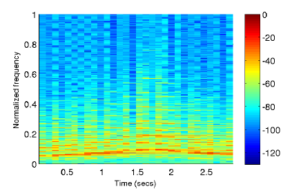
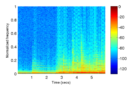
Figure 1: (Color online only) Spectrograms of the Flute Exercise clip (left) $N=65536$ samples at 22050 Hz, and that of the Classic Guitar, $N=262144$ samples at 44100Hz. Each spectrogram was produced using a Hamming window of length $4096$ samples and 50$\%$ overlap.

The approximation of all the clips in Table 1 was carried out for partitions corresponding to $N_{b}$ equal to 512, 1024, 2048, 4096, 8192, and 16384 samples. For space limitation only the sparsity results corresponding to all those values of $N_{b}$ are shown for the first two clips of the table. Fig. 1 gives the classic spectrogram for the Flute Exercise and Classical Guitar. Fig. 2 shows the values of the SR for those clips, as a function of the partition unit size $N_{b}$.

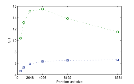
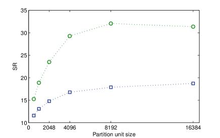
Figure 2: (Color online only) SR, for the Flute Exercise clips (left) and Classical Guitar (right) corresponding to values of $N_{b}$ equal to 512, 1024, 2048, 4096, 8192, and 16384 samples. The squares are the SR values obtained with the orthogonal basis $\mathcal{B}^{c}$. The circles are the results produced by the mixed dictionary $\mathcal{D}^{cs}$, redundancy four, by means of the proposed algorithm.

As seen in the figures, for all the values of $N_{b}$, the gain in sparsity produced by the dictionary (represented by the circles in Fig. 2) in relation to the best result for the basis (squares in those figures) is very significant. Table 1 shows the values of SR for the clips listed in the first column, using the basis $\mathcal{B}^{c}$ and the dictionary $\mathcal{D}^{cs}$ with the methods MP and SPMP. The value of $N_{b}$ is set as that producing the best SR for the orthogonal basis $\mathcal{B}^{c}$ which, as illustrated in the left graph of Fig. 2, is not always the optimal value for the dictionary approach. The implementation of the MP algorithm via FFT, which we call MPTrgFFT, is ready realized simply by deactivating the self projection step.

Clip	$N_{b}$	SR ($\mathcal{B}^{c}$)	SR (MP)	SR (SPMP)
Flute Exercise	8192	6.5	11.8	13.9
Classic Guitar	16384	18.7	26.6	31.4
Rock Piano	2048	6.9	10.2	12.0
Pop Piano	8192	11.7	15.1	18.0
Rock Ballad	8192	6.8	8.9	10.5
Bach Piano	4096	11.8	14.8	17.4
Trumpet Solo	8192	8.3	11.9	14.7
Himno del Riego	4096	4.9	7.6	8.9
Oboe in C	16384	13.7	44.1	53.5
Classical Romance	8192	7.2	11.2	13.4
Jazz Organ	8192	18.7	22.5	28.1
Marimba Jazz	1024	11.8	15.3	18.6
Begana	2048	8.5	10.0	12.0
Vibraphone	2048	12.7	20.1	23.8
Polyphon	4096	3.7	6.1	7.1

Table 1: SR obtained with the basis $\mathcal{B}^{c}$ and the dictionary $\mathcal{D}^{cs}$, through the MP and SPMP methods, for the clips listed in the first column. The value of the partition unite $N_{b}$ is the one corresponding to the best SR result with the basis $\mathcal{B}^{c}$ when $N_{b}$ takes the values 512, 1024, 2048, 4096, 8192, and 16384.

The clips in Table 1 are played with a variety of instruments. The sampling frequencies are: 22050 Hz for the Flute Exercise and Himno del Riego, 48000 Hz for the Polyphon, and 44100 Hz for all the other clips. The SR varies significantly, from the sparsest clip (Oboe in C) to the least sparse one (Polyphon). Nevertheless, the gain in sparsity obtained with the trigonometric dictionaries, in relation to the best orthogonal basis, is in most cases very significant. Notice that drums are not included in the list. The reason being that drum loops are best approximated when the partition size is considerably smaller than for the instruments in Table 1. Hence, the proposed algorithm is not of particular help in that case. On the contrary, as discussed in Sec. I, a method linking the approximation of the elements in the partition through a global constraint on sparsity, or quality, is much better suited to that situation (Rebollo-Neira 2016a). The same holds true for speech signals. Additionally, we understand that drum loops do not fall within the class of music that can be sparsely represented only with trigonometric atoms of the type we are considering here.

In order to compare the improvement in SR produced by the SPMP method ($\text{SR}_{\text{SPMP}}$) over the MP one ($\text{SR}_{\text{MP}}$) we defined the relative gain in sparsity as follows:

$$G=\frac{\text{SR}_{\text{SPMP}}-\text{SR}_{\text{MP}}}{\text{SR}_{\text{MP}}}100\%$$ (15)

For the results of Table 1 the mean value gain is $\bar{G}=19.4\%$ with standard deviation of 2.4%.

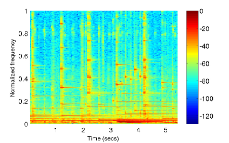
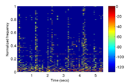
Figure 3: (Color online only) The left graph is the classic spectrogram of the Polyphon clip obtained with a Hamming window of length $4096$ samples and 50$\%$ overlap. The right graph is the sparser version of the spectral decomposition, realized by the trigonometric dictionary and the SPMPTrgFFT algorithm, on a partition of disjoint units of size $N_{b}=4096$.

Fig. 3 gives a visual representation of the implication of the SR value. The left graphs is a classic spectrogram for the Polyphon clip, which has been re-scaled to have the maximum value equal to one. The right graph is the sparse spectral representation constructed with the outputs of the SPMPTrgFFT algorithm (also re-scaled to have maximum value equal to one). Because the spectrograms are given in dB, and the sparse one has zero entries, the value $10^{-13}$ was added to all the spectral power outputs to match scales.

In order to give a description of local sparsity we consider the local sparsity ratio $sr_{q}=\frac{N_{b}}{k_{q}},\,q=1,\ldots,Q$, where $k_{q}$ is the number of coefficients in the decomposition of the $q$-block and $N_{b}$ the size of the block. For illustration convenience the graphs in Figs. 4 depict the inverse of this local measure. The points in those figures represent the values $1/sr_{q},\,q=1,\ldots,Q$. Each of these values is located in the horizontal axis at the center of the corresponding block. For each signal the size of the block is taken to be the value $N_{b}$ yielding the largest SR with the dictionary approach, for that particular signal.

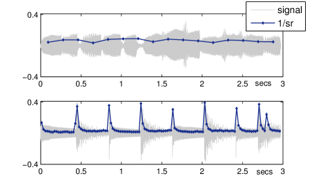
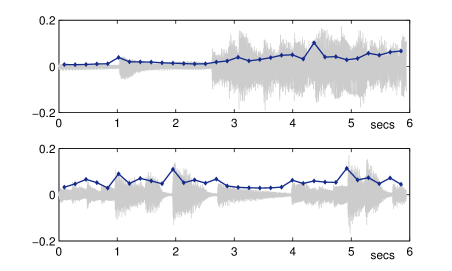
Figure 4: (Color online only) The points joined by the darker line in all the graphs are the values of the inverse local sparsity ratio $1/sr_{q},\,q=1,\ldots,Q$. The top graphs correspond to the Flute (left) and Classic Guitar clips. The bottom graphs correspond to the Marimba (left) and Pop Piano clips. The lighter lines represent the signals.

The lighter lines in all the graphs of Fig. 4 represent the Flute, Marimba Classic Guitar and Pop Piano clips. It is interesting to see that each if the darker lines joining the inverse local sparsity points follows, somewhat, the shape of signal’s envelop. This is particularly noticeable when a transient occurs.

As opposed to the method of Serra and Smith (1990), which would model a possible component of a sound clip by tracking the evolution of some frequencies along time, but in general would produce a significant residue, the goal of the proposed sparse spectral representation is to achieve high quality reconstruction. As indicated by the points in the graphs of Fig. 4, for some signals this is attained by a decomposition of low local sparsity in particular blocks. Notice, however, that a signal exhibiting such picks of inverse local sparsity may produce, on the whole, a SR which is higher than the SR of a signal endowed with more uniform local sparsity, e.g. Flute vs Marimba and Pop Piano. The clips of Table 1 are all played with single instruments. The rather high value of SNR (35dB) is set to avoid noticeable loss or artifacts in the signal reconstruction, which might be easy to detect due to the nature of the sound. Nevertheless, for the clips of Table 2, which are played by multiple instruments, for SNR$=$25dB (and even lower) we do not perceive loss or artifacts. Hence, the sparsity results of Table 2 correspond to SNR=25dB. Overestimating the required SNR for high quality recovery would produce a significant reduction of the SR values.

Clip	SR ($\mathcal{B}^{c}$)	SR (MP)	SR (SPMP)
Classic Music (sextet)	12.2	16.2	18.4
Piazzola Tango (quartet)	10.7	13.8	15.7
Opera (female voice)	5.6	7.5	8.3
Opera (male voice)	9.2	12.0	13.5
Bach Fugue (orchestral version)	8.2	12.4	14.1
Simple Orchestra	13.1	17.6	19.8

Table 2: SR obtained with the basis $\mathcal{B}^{c}$ and the dictionary $\mathcal{D}^{cs}$, through the MP and SPMP methods, for the clips listed in the first column. The partition unite size is in all the cases $N_{b}=4096$ and the sampling frequency 44100 Hz.

For the results of Table 2 the mean value gain in SR (c.f. (15)) is $\bar{G}=12.8\%$ with standard deviation of $1.2\%$.

Remarks on computational complexity: The increment in the computational complexity of SPMPTrgFFT with respect to MPTrgFFT is a factor which accounts for the iterations realizing the self-projections. In order to estimate the complexity we indicate by $\overline{\overline{\kappa}}$ the double average of the number of iterations in the projection step. More specifically, indicating by $\kappa_{k}$ the number of iterations in the $k$-term approximation of a fixed segment $q$, $\overline{\kappa}_{q}=\frac{1}{k_{q}}\sum_{k=1}^{k_{q}}\kappa_{k}$ and ${\displaystyle{\overline{\overline{\kappa}}=\frac{1}{Q}\sum_{q=1}^{Q}\overline{\kappa}_{q}}}$.

The value of $\overline{\overline{\kappa}}$ gives an estimation of the SPMPTrgFFT complexity: O($\overline{\overline{\kappa}}KM\log_{2}M$). Since for a dictionary of redundancy $r$ the number of elements is $M=rN_{b}$, in order to make clearer the influence of the segment’s length in the complexity, this can be expressed as O($\overline{\overline{\kappa}}KrN_{b}\log_{2}rN_{b})$. The computational complexity of plain MPTrgFFT is given by the complexity of calculating inner products via FFT, i.e. O($KrN_{b}\log_{2}rN_{b})$. Hence $\overline{\overline{\kappa}}$ gives a measure of the increment of complexity introduced by the projections to achieve the desired optimality in the coefficients of the approximation. Fig. 5 shows the values of $\overline{\overline{\kappa}}$ as a function of the segment’s length $N_{b}$. The triangles correspond to the Flute Exercise clip the starts to the Classic Guitar clip. Notice that for the Flute Exercise the value of $\overline{\overline{\kappa}}$ augments significantly for the two larger values of $N_{b}$, while remains practically constant for the Classic Guitar. This feature is in line with the fact that, as seen in Fig 2, the SR for those values of $N_{b}$ is practically constant for the Classic Guitar, but decreases for the Flute Exercise.

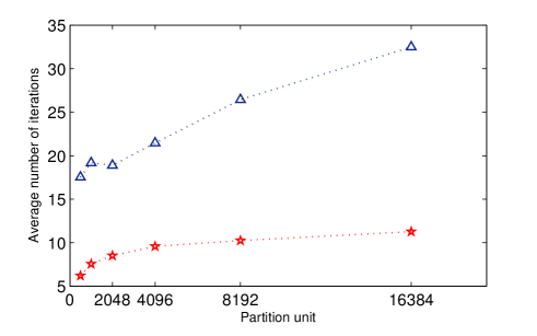
Figure 5: (Color online only) Average number of the iterations, $\overline{\overline{\kappa}}$, for realizing the projection step procedure (Algorithm 5) corresponding to partition units of length $N_{b}$ equal to 512, 1024, 2048, 4096, 8192, and 16384 samples. The triangles are the values for the flute clip and the starts for the classic guitar.

IV Conclusions

A dedicated method for sparse spectral representation of music sound has been presented. The method was devised for the representation to be realized outside the orthogonal basis framework. Instead, the spectral components are selected from an overcomplete trigonometric dictionary. The suitability of these dictionaries for sparse representation of melodic music, by partitioning, was illustrated on a number of sound clips of different nature. While the quality of the reconstruction is an input of the algorithm, the method is conceived to achieve high quality recovery. Hence, in order to benefit sparsity results the signal partition is realized without overlap. The approach has been shown to be worth applying to improve sparsity within the class of signal which are compressible in terms of a trigonometric basis. The achieved sparsity is theoretically equivalent to that produced by the OMP approach with the identical dictionary. The numerical equivalence of both algorithms was verified when possible.

In order to facilitate the application of the approach we have made publicly available the MATLAB version of Algorithms 1-6 on a dedicated web page¹. It is appropriate to stress, though, that the routines are not intended to be an optimized implementation of the method. On the contrary, they have been produced with the intention of providing an easy to test form of the approach. We hope that the MATLAB version of the algorithms will facilitate their implementation in appropriate programming languages for practical applications.

Acknowledgements

We are grateful to three anonymous reviewers for many comments and suggestions for improvements to previous versions of the manuscript. We are also grateful to Xavier Serra who has kindly let us have a MATLAB function for the implementation of their method (Serra and Smith, 1990).

Notes

1. 1 http://www.nonlinear-approx.info/examples/node02.html

Appendix A

  Input:$\,\mathbf{R}\in\mathbb{R}^{N}$, $M$, number of elements in the dictionary, and Case (I , II, or III).

  {Computation of the inner products $\mathbf{IP}=\langle\mathbf{d},\mathbf{R}\rangle\in\mathbb{C}^{M}$}

  Case I

  $\mathbf{IP}={\rm{FFT}}(\mathbf{R},M$)$\frac{1}{\sqrt{N}}$,

  Case II, III (c.f. (13), (14))

  {Computation of auxiliary vector $\mathbf{Aux}\in\mathbb{C}^{2M}$ to compute $\mathbf{IP}$.}

  $\mathbf{Aux}={\rm{FFT}}(\mathbf{R},2M)$

  Case II

  $IP(n)=\frac{1}{w^{c}(n)}\operatorname{Re}(e^{\imath\frac{\pi(n-1)}{M}}Aux(n)),\,n=1,\ldots,M$

  Case III

  $IP(n-1)=-\frac{1}{w^{s}(n)}\operatorname{Im}(e^{\imath\frac{\pi(n-1)}{M}}Aux(n)),\,n=2,\ldots,M+1$

Algorithm 1 Computation of inner product with a trigonometric dictionary via FFT. IPTrgFFT procedure: $[\mathbf{IP}]=$IPTrgFFT($\mathbf{R},M,$ Case)

  Input:  Index $\ell_{k}$, number of elements in the dictionary $M$, atom’s dimension $N$, Case (I, II, III or IV).

  Output:  Atom $\mathbf{d}_{\ell_{k}}$.

  {Generation of the atom, $\mathbf{d}_{\ell_{k}}$, according to the Case}

  if Case=IV then

     $M\leftarrow\frac{M}{2}$

  end ifCase I${\displaystyle{d_{\ell_{k}}(j)=\frac{1}{\sqrt{N}}e^{\imath\frac{{2\pi(j-1)(\ell_{k}-1)}}{M}},\quad j=1,\ldots,N}}$ Case II (and Case IV if $\ell_{k}\leq\frac{M}{2}$) ${\displaystyle{d_{\ell_{k}}(j)=\frac{1}{w^{c}(\ell_{k})}\,\cos({\frac{{\pi(2j-1)(\ell_{k}-1)}}{2M}}),\quad j=1,\ldots,N}}$Case III (and Case IV if ${\displaystyle{\ell_{k}>\frac{M}{2}}}$) ${\displaystyle{d_{\ell_{k}}(j)=\frac{1}{w^{s}(\ell_{k})}\,\sin({\frac{{\pi(2j-1)\ell_{k}}}{2M}}),\quad j=1,\ldots,N}}$

Algorithm 2 Generation of an atom, given the index and the dictionary type. Trigonometric Atom procedure: $[\mathbf{d}_{\ell_{k}}]$=TrgAt($\ell_{k},M,N,$ Case)

Algorithm 3 Atom Selection via FFT. AtSelFFT procedure: $[\ell_{k},c(\ell_{k})]=$AtSelFFT($\mathbf{R},M,$ Case)

  Input:  Residual $\mathbf{R}\in\mathbb{R}^{N}$, $M$ number of elements in the dictionary, and Case (I, II, III, or IV)

  Output: Index of the selected atom $\ell_{k}$, and MP coefficient $c(\ell_{k})=\langle\mathbf{d}_{\ell_{k}},\mathbf{R}\rangle$ calculated via FFT. {Call IPTrgFFT procedure, Algorithm 11, to calculate inner products}

  Case I $\mathbf{IP}$=IPTrgFFT($\mathbf{R},M,$ Case I),

  Cases II and III $\mathbf{IP}$=IPTrgFFT($\mathbf{R},M,$ Case), {Selection of the new atom and evaluation of the MP coefficient} ${\displaystyle{\ell_{k}=\operatorname*{arg\,max}_{\begin{subarray}{c}n=1,\ldots,M\end{subarray}}|IP(n)|}}$ $c(\ell_{k})=IP(\ell_{k})$

  Case IV $M\leftarrow\frac{M}{2}$

  $\mathbf{IP}^{c}$=IPTrgFFT($\mathbf{R},M$, Case II)$\mathbf{IP}^{s}$=IPTrgFFT($\mathbf{R},M,$ Case III) $\displaystyle{\nu=\operatorname*{max}(|IP^{c}(\ell^{c})|,|IP^{s}(\ell^{s})|),\,\,\text{with}\,\,\ell^{c}=\operatorname*{arg\,max}_{\begin{subarray}{c}n=1,\ldots,M\end{subarray}}|IP^{c}(n)|\,\,\text{and\,\,}\ell^{s}=\operatorname*{arg\,max}_{\begin{subarray}{c}n=1,\ldots,M\end{subarray}}|IP^{s}(n)|}$

  if $\nu=|IP^{s}(\ell^{s})|$ then

     $\ell_{k}=\ell^{s}+M$ and $c(\ell_{k})=IP^{s}(\ell^{s})$

  else

     $\ell_{k}=\ell^{c}$ and $c(\ell_{k})=IP^{c}(\ell^{c})$

  end if

Algorithm 4 Atom Re-Selection via FFT. AtReSelFFT procedure: $[\ell,c(\ell)]$=AtReSelFFT($\mathbf{R},M,\Gamma,$ Case)

  Input:  Residue $\mathbf{R}\in\mathbb{R}^{N}$, number of dictionary’s elements, $M$, set of indices of the selected atoms $\Gamma=\{\ell_{n}\}_{n=1}^{k}$ (if Case=IV both, $\Gamma^{c}$, indices for atoms in $\mathcal{D}^{c}$, and $\Gamma^{s}$, indices for atoms in $\mathcal{D}^{s}$).

  Output:  Re-Selected index $\ell$ (out of the set $\Gamma$) and corresponding MP coefficient $c(\ell)=\langle\mathbf{d}_{\ell},\mathbf{R}\rangle,\ell\in\Gamma$, calculated via FFT.

  Case I $\mathbf{IP}$=IPTrgFFT($\mathbf{R},M,$ Case I),

  Cases II and III $\mathbf{IP}$=IPTrgFFT($\mathbf{R},M,$ Case ), {Selection of the index $\ell\in\Gamma$} ${\displaystyle{\ell=\operatorname*{arg\,max}_{\begin{subarray}{c}n\in\Gamma\end{subarray}}|IP(n)|}}$ $c(\ell)=IP(\ell)$

  Case IV $M\leftarrow\frac{M}{2}$

  $\mathbf{IP}^{c}$=IPTrgFFT($\mathbf{R},M,$ Case II)$\mathbf{IP}^{s}$=IPTrgFFT($\mathbf{R},M,$ Case III) $\displaystyle{\nu=\operatorname*{max}(|IP^{c}(\ell^{c})|,|IP^{s}(\ell^{s})|,\,\,\text{with}\,\,\ell^{c}=\operatorname*{arg\,max}_{\begin{subarray}{c}n\in\Gamma^{c}\end{subarray}}|IP^{c}(n)|\,\,\text{and\,\,}\ell^{s}=\operatorname*{arg\,max}_{\begin{subarray}{c}n\in\Gamma^{s}\end{subarray}}|IP^{s}(n)|}$

  if $\nu=|IP^{s}(\ell^{s})|$ then

     $\ell=\ell^{s}+M$ and $c(\ell)=IP^{s}(\ell^{s})$

  else

     $\ell=\ell^{c}$ and $c(\ell)=IP^{c}(\ell^{c})$

  end if

  Input:  Residue $\mathbf{R}\in\mathbb{R}^{N}$, number of elements in the dictionary, $M$, vectors $\mathbf{c}$ with the coefficients in the $k$-term approximation, set $\Gamma$ of selected indices up to iteration $k$, tolerance for the numerical error of the projection $\epsilon$, and Case (I, II, III, or IV).

  Output:  Updated residue, $\mathbf{\tilde{R}}\in\mathbb{R}^{N}$, orthogonal to ${\mbox{\rm{span}}}\{\mathbf{d}_{n}\}_{n\in\Gamma}$ and updated coefficients $\mathbf{\tilde{c}}$ accounting for the projection. {Set $\mu=2\epsilon$ to start the algorithm}

  while $\mu>\epsilon$ do

     {Select one index from $\Gamma$ to construct the approximation of $\mathbf{R}$ in ${\mbox{\rm{span}}}\{\mathbf{d}_{n}\}_{n\in\Gamma}$}

     $[\ell,\tilde{c}(\ell)]$=AtReSelFFT($\mathbf{R},M,\Gamma,$ Case) {Generate the selected atom $\mathbf{d}_{\ell}$}

     $\mathbf{d}_{\ell}$=TrgAt($\ell,M,N$, Case). {Update residue}

     ${\displaystyle{\mathbf{R}\leftarrow\mathbf{R}-\tilde{c}(\ell)\mathbf{d}_{\ell}}}$ {Since $\mathbf{R}$ is vector of real numbers}

     if Case = I then

         $\ell^{\prime}=M-\ell+2$, $\mathbf{d}_{\ell^{\prime}}$=TrgAt($\ell^{\prime},M,N$, Case), ${\displaystyle{\mathbf{R}}\leftarrow\mathbf{R}-\tilde{c}^{\ast}(\ell)\mathbf{d}_{\ell^{\prime}}}$

     end if

     $\mu=|\tilde{c}(\ell)|$ {Update coefficient} $c(\ell)\leftarrow c(\ell)+\tilde{c}(\ell)$

     if Case = I then

        $c(M-\ell+2)\leftarrow c^{\ast}(\ell)$

     end if

  end while{Rename coefficients and residue to match the output variables}

  $\mathbf{\tilde{c}}=\mathbf{c},\,\mathbf{\tilde{R}}=\mathbf{R}$

Algorithm 5 Orthogonal Projection via FFT. ProjMPTrgFFT procedure: $[\mathbf{\tilde{R}},\mathbf{\tilde{c}}]$=ProjMPTrgFFT($\mathbf{R},M,\mathbf{c},\Gamma,\epsilon,$ Case)

  Input:  Data $\mathbf{f}\in\mathbb{R}^{N}$, $M$, number of elements in the dictionary, approximation error $\rho>0$ and tolerance $\epsilon>0$ for the numerical realization of the projection Case (I , II, III, or IV).

  Output:  Approximated data $\mathbf{f}^{k}\in\mathbb{R}^{N}$. Coefficients in the atomic decomposition, $\mathbf{c}$, Indices labeling the selected atoms $\Gamma=\{\ell_{n}\}_{n=1}^{k}$.

  {Initialization}

  Set$\,\,\Gamma\,=\,\{\emptyset\},\quad\mathbf{f}^{0}\,=\,0,\quad\mathbf{R}^{0}\,=\,\mathbf{f},\,\quad k\,=\,0,\quad\mu=2\rho$

  {Begin the algorithm}

  while $\mu>\rho$ do

     $k=k+1$ {Select index $\ell_{k}$ and calculate $c(\ell_{k})$}

     $[\ell_{k},c(\ell_{k})]$=AtSelFFT($\mathbf{R}^{k-1},M,$ Case) {Generate the atom $\d{(}{\ell_{k}})$} $\mathbf{d}_{\ell_{k}}$=TrgAt$(\ell_{k},M,N,$ Case)

     Updated $\Gamma\leftarrow\Gamma\cup\ell_{k}$ {Calculate approximation and residue}

     $\mathbf{f}^{k}=\mathbf{f}^{k-1}+c(\ell_{k})\mathbf{d}_{\ell_{k}},$ and $\mathbf{R}^{k}=\mathbf{f}-\mathbf{f}^{k}$ {Subtract from $\mathbf{R}^{k}$ the component in ${\mbox{\rm{span}}}\{\mathbf{d}_{n}\}_{n\in\Gamma}$} [$\mathbf{\tilde{R}}^{k},\mathbf{\tilde{c}}$]=ProjMPTrgFFT($\mathbf{R}^{k},M,\mathbf{c},\Gamma,\epsilon,$ Case) {Update residue, approximation, coefficients, and error}

     $\mathbf{R}^{k}=\mathbf{\tilde{R}}^{k},\mathbf{f}^{k}=\mathbf{f}-\mathbf{R}^{k};\mathbf{c}=\mathbf{\tilde{c}},\mu=\|\mathbf{R}^{k}\|$

  end while

Algorithm 6 Main Algorithm for the proposed SPMP method dedicated to trigonometric dictionaries and implemented via FFT. Procedure SPMPTrgFFT: $[\mathbf{f}^{k},\mathbf{c},\Gamma]=$ SPMPTrgFFT($\mathbf{f},M,\rho,\epsilon,$ Case)

References

- [1] J. F. Alm and J. S. Walker, “Time-Frequency Analysis of Musical Instruments”, SIAM Review, 40, 457–476 (2002).
- [2] R. Baraniuk, “Compressive sensing”, IEEE Signal Processing Magazine, 24, 118–121, (2007).
- [3] R. Baraniuk, “More Is less: Signal processing and the data deluge”, Science, 331, 717 – 719 (2011).
- [4] J. Candès, J. Romberg, and T. Tao, “Robust uncertainty principles: exact signal reconstruction from highly incomplete frequency information,” IEEE Trans. Inf. Theory, 52, 489 –509 (2006).
- [5] E. Candès and M. Wakin, “An introduction to compressive sampling”, IEEE Signal Processing Magazine, 25, 21 – 30 (2008).
- [6] M. Davy and S. J. Godsill, “Bayesian Harmonic Models for Musical Signal Analysis”, in Bayesian Statistics 7, Oxford University Press, 105–124, 2002.
- [7] I. Daubechies, “Ten Lectures on Wavelets”, SIAM, 55–103, 1992.
- [8] D. L. Donoho, “Compressed sensing”, IEEE Trans. Inf. Theory,52, 1289–1306 (2006).
- [9] N. Fletcher and T. Rossing, “The Physics of Musical Instruments”, Springer-Verlang, Berling, 1–131, 1998.
- [10] J. H. Friedman and W. Stuetzle, “Projection Pursuit Regression”, Journal of the American Statistical Association, 76, 817– 823 (1981).
- [11] R. Gribonval and E. Bacry, “Harmonic Decomposition of Audion Signals with Matching Pursuit”, IEEE Trans. on Signal Processing, 51 (2003).
- [12] L. K. Jones, “On a conjecute of Huber concerning the convergence of Projection Pursuit Regression”, Ann. Statist. 15, 880–882 (1987).
- [13] S. G. Mallat and Z. Zhang, “Matching Pursuits with Time-Frequency Dictionaries”, IEEE Trans. Signal Process., 41, 3397–3415 (1993).
- [14] B. K. Natarajan, “Sparse Approximate Solutions to Linear Systems”, SIAM Journal on Computing, 24, 227–234 (1995).
- [15] Y.C. Pati, R. Rezaiifar, and P.S. Krishnaprasad, “Orthogonal matching pursuit: recursive function approximation with applications to wavelet decomposition,” Proc. of the 27th ACSSC,1, 40–44 (1993).
- [16] J. R. Partington, “Interpolation, Identification, and Sampling”, London Mathematical Society Monographs New Series 17, Oxford University Press, 1997.
- [17] L. Rebollo-Neira and D. Lowe, “Optimized orthogonal matching pursuit approach”, IEEE Signal Process. Letters, 9, 137–140 (2002).
- [18] L. Rebollo-Neira, ‘Constructive updating/downdating of oblique projectors: a generalization of the Gram-Schmidt process”, Journal of Physics A: Mathematical and Theoretical, 40, 6381–6394 (2007).
- [19] L. Rebollo-Neira and J. Bowley, “Sparse representation of astronomical images”, J. Opt. Soc. Am. A, 20, 1175–1178 (2013).
- [20] L. Rebollo-Neira, “Cooperative Greedy Pursuit Strategies for Sparse Signal Representation by Partitioning”, Signal Processing, 125, 365–375 (2016a).
- [21] L. Rebollo-Neira, “Trigonometric dictionary based codec for music compression with high quality recovery,” http://arxiv.org/abs/1512.04243 (2016b).
- [22] X. Serra and J. Smith III, “Spectral Modeling Synthesis: A Sound Analysis/Synthesis Based on a Deterministic plus Stochastic Decomposition”, Computer Music Journal, 14, 12–24 (1990).
- [23] J. O. Smith III, “Spectral Audio Signal Processing”, W3K Publishing, 231–253, 2011.
- [24] J. Wolfe, J. Smith, J. Tann, N. H. Fletcher, “Acoustic impedance spectra of classical and modern flutes”, Journal of Sound and Vibration, 243, 127–144 (2001).
- [25] R. Young, “An introduction to nonharmonic Fourier series”, Academic Press, 154–169, 1980.