Squeezed between shells? On the origin of the Lupus I molecular cloud

Abstract

Context. The Lupus I cloud is found between the Upper-Scorpius (USco) and the Upper-Centaurus-Lupus (UCL) sub-groups of the Scorpius-Centaurus OB-association, where the expanding USco H I shell appears to interact with a bubble currently driven by the winds of the remaining B-stars of UCL.

Aims. We want to study how collisions of large-scale interstellar gas flows form and influence new dense clouds in the ISM.

Methods. We performed LABOCA continuum sub-mm observations of Lupus I that provide for the first time a direct view of the densest, coldest cloud clumps and cores at high angular resolution. We complemented those by Herschel and Planck data from which we constructed column density and temperature maps. From the Herschel and LABOCA column density maps we calculated PDFs to characterize the density structure of the cloud.

Results. The northern part of Lupus I is found to have on average lower densities and higher temperatures as well as no active star formation. The center-south part harbors dozens of pre-stellar cores where density and temperature reach their maximum and minimum, respectively. Our analysis of the column density PDFs from the Herschel data show double peak profiles for all parts of the cloud which we attribute to an external compression. In those parts with active star formation, the PDF shows a power-law tail at high densities. The PDFs we calculated from our LABOCA data trace the denser parts of the cloud showing one peak and a power-law tail. With LABOCA we find 15 cores with masses between 0.07 and $1.71\,M_{\odot}$ and a total mass of $\approx 8\,M_{\odot}$. The total gas and dust mass of the cloud is $\approx 164\,M_{\odot}$ and hence $\sim 5\%$ of the mass is in cores. From the Herschel and Planck data we find a total mass of $\approx 174\,M_{\odot}$ and $\approx 171\,M_{\odot}$, respectively.

Conclusions. The position, orientation and elongated shape of Lupus I, the double peak PDFs and the population of pre-stellar and protostellar cores could be explained by the large-scale compression from the advancing USco H I shell and the UCL wind bubble.

1 Introduction

In the current picture of the dynamic interstellar medium (ISM), molecular cloud formation is attributed to collisions of large-scale flows in the ISM (see review by Dobbs et al. 2014, and references within). Such flows can be driven by stellar feedback processes (e.g. UV-radiation and winds) and supernovae. At the interface of the colliding flows, compression, cooling, and fragmentation of the diffuse atomic medium produces cold sheets and filaments that later may become molecular and self-gravitating and dominate the appearance of the ISM as observed today (see review by André et al. 2014). In this picture the fast formation (and dispersion) of molecular clouds and the often simultaneous onset of star formation within (see Hartmann et al. 2001; Vázquez-Semadeni et al. 2007; Banerjee et al. 2009; Gómez & Vázquez-Semadeni 2014) appears plausible.

One example of such a large-scale flow is an expanding shell or super-shell around e.g. an OB-association or in general driven by multiple stellar feedback of a star cluster or association (see review by Dawson 2013). Molecular clouds may then either form inside the wall of such a shell (Dawson et al. 2011) or at the interface region when two such shells collide with each other. The latter has been recently investigated by Dawson et al. (2015) for a young giant molecular cloud (GMC) at the interface of two colliding super-shells. From the comparison of CO observations with high-resolution 3D hydrodynamical simulations they found that the GMC assembled into its current form by the action of the shells.

The Scorpius-Centaurus OB-association (Blaauw 1964; de Zeeuw et al. 1999; Preibisch et al. 2002; Preibisch & Mamajek 2008, Sco-Cen) is the closest site of recent massive star formation to us and it consists of three sub-groups with different ages and well known stellar populations down to $2\,M_{\odot}$ (de Bruijne 1999). The oldest one is the the Upper Centaurus-Lupus (UCL) sub-group with an age of $\sim 17$ Myr harboring 66 B-stars. With an age of $\sim 15$ Myr the Lower Centaurus Crux (LCC) sub-group is somewhat younger and contains 42 B-stars. The youngest sub-group is Upper-Scorpius (USco) with an age of $\sim 5$ Myr and consisting of 49 B-stars.

The feedback of the numerous massive stars in Sco-Cen probably cleared the inner region of the association from diffuse matter creating expanding loop-like H I shells around each of the sub-groups of the association (de Geus 1992). At the edge of the USco shell several dense molecular clouds with very young ($\leq 1-2$ Myr) stellar populations are found. Of those the most prominent ones are the Lupus I cloud (near the western edge of the shell) and the $\rho$ Oph cloud (near the eastern edge).

The Lupus I molecular cloud complex (for an overview see Comerón 2008) is found at a distance of 150 pc and consists of a $\approx 2.6\degr\times 0.6\degr$ (corresponds to a physical size of $\approx 6.8\times 1.6$ pc) main filament extending in a north to south direction (Galactic coordinates) and a ring-like structure of $\sim 0.6\degr$ in diameter west of the main filament (towards UCL; see Tothill et al. 2009). Recently Matthews et al. (2014) noted also two smaller secondary filaments of which one is about half a degree long and runs perpendicular to the main filament and seems to connect with it in the south. The other one is about a degree long and lies south-west of the main filament extending from the southern end of the main filament to the ring-like structure.

In this work we concentrate our analysis only on the main filament commonly seen in all observations. We will refer to it as Lupus I or the Lupus I filament.

The cloud is found between the USco and the UCL sub-groups at a location where the expanding USco shell appears to interact with a bubble currently powered by the winds of the remaining B-stars of UCL. With its close distance Lupus I represents a good candidate where we can study how such a collision process may form and influence new dense clouds in the ISM.

Lupus I has been mapped as part of several large surveys like the Herschel Gould-belt survey (André et al. 2010; Rygl et al. 2013) and the Spitzer Legacy Program ’From molecular clouds to planet-forming disks’ (c2d; Chapman et al. 2007; Merín et al. 2008). These near-infrared to far-infrared surveys revealed the population of young stellar objects (YSOs) within the cloud showing that it is dominated by pre-stellar and protostellar cores indicating an on-going star formation event. Rygl et al. (2013) found that the star formation rate (SFR) is increasing over the past $0.5-1.5$ Myr and Merín et al. (2008) estimated a SFR of $\rm 4.3\,M_{\odot}\,Myr^{-1}$ for Lupus I from their Spitzer data.

Extinction maps of Lupus I have been created by various authors using different methods. Cambrésy (1999) created an extinction map based on optical star counts with a resolution of a few arc-minutes. Using 2MASS data Chapman et al. (2007) created a visual extinction map with a $2\arcmin$ resolution. Also from 2MASS data a wide field extinction map of Lupus I has been presented by Lombardi et al. (2008). It allowed extinction measurements down to $A_{K}=0.05$ mag, but had a resolution of $3\arcmin$. Merín et al. (2008) created extinction maps from their Spitzer data by estimating the visual extinction towards each source classified as a background star, based on their spectral energy distribution (SED) from 1.25 to $24\,\mu$m. Their maps had a resolution of $2-5\arcmin$. Rygl et al. (2013) created a column density map of dust emission in Lupus I from their Herschel data by making a modified black body fit for each pixel in the four bands from $160-500\,\mu$m. The resulting resolution was $36\arcsec$.

Here we present a far-infrared and sub-mm analysis of the Lupus I cloud based on newly obtained APEX/LABOCA sub-mm continuum data at $870\,\mu$m and complementing those with Herschel and Planck archival data. In Sec. 2 we briefly describe the observations used and their data reduction process. Sec. 3 gives an overview of the methods used to create column density maps and probability distribution functions (PDFs) from the observations. We present and discuss our results in Sec. 4. In Sec. 5 we consider the surroundings of Lupus I and the influence of large-scale processes on the cloud. Finally, we summarize and conclude our paper in Sec. 6.

2 Observations and data reduction

2.1 LABOCA data

The sub-mm continuum observations of Lupus I were performed with the APEX 12-m telescope located in the Chilean Atacama desert (Güsten et al. 2006). We used the LArge APEX BOlometer CAmera (LABOCA, Siringo et al. 2009) which operates in the atmospheric window at $870\,\mu$m (345 GHz). The angular resolution is 19.2″(HPBW), and the total field of view is 11.4′. At the distance of Lupus I (150 pc) the angular resolution corresponds to a spatial scale of $\sim 2800$ AU ($\sim 0.01$ pc). This is sufficient to resolve the structure of molecular cores.

The LABOCA observations of Lupus I were obtained in Max-Planck and ESO Periods 91 and 92, on 24th March, 31st August, 12th, 13th September 2013, and 31st March 2014 (PI: B. Gaczkowski). They were performed in the on-the-fly (OTF) mode, scanning perpendicular as well as along the filament’s major axis with a random position angle to the axis for each scan to reduce striping effects and improve the sampling. The total observing time was 11.3 hours and the weather conditions good to average.

Data reduction included standard steps for sub-millimeter bolometer data, using the BoA software package (Schuller 2012). First, data were converted from instrumental count values to a Jansky scale using a standard conversion factor, then a flatfield correction (derived from scans of bright, compact sources) was applied. Corrections for atmospheric opacity were derived from skydips taken every 1-2 hours, and finally residual correction factors were determined from observations of planets and secondary calibrator sources. Data at the turning points of the map were flagged, as well as spikes. The data from the individual bolometers were then corrected for slow amplitude drifts due to instrumental effects and atmosphere by subtracting low-order polynomials from the time-stream data. Short timescale sky brightness variations (sky-noise) was corrected by removing the correlated (over a large number of bolometers) signal in an iterative fashion. Then the time-stream data were converted into sky-brightness maps for each scan, and finally all scans combined into one map.

The removal of the correlated sky variations is known to filter out also astronomical emission from extended sources, usually leading to negative artifacts surrounding bright emission structures. In order to recover some of the extended emission, an iterative source modeling procedure was applied, using the result from the previous iteration to construct an input model for the following iteration. To construct the model, the previous map was smoothed, all pixels below a pixel value of 0 set to 0, and the map smoothed again. In the following iteration, the model is subtracted from the time-stream data before de-spiking, baseline subtraction, and sky-noise removal, and added back to the data stream afterwards, before the new map is created. This procedure effectively injects artificial flux into the mapped area and is prone to create runaway high surface brightness areas especially in regions without significant astronomical signal and low signal-to-noise. For that reason, the model image was set entirely to 0 in areas of the map with poor coverage, below a certain threshold in rms (basically the map edges), and the procedure was stopped after 25 iterations. Typically, structures on scales of the order of $3-4\arcmin$ can be recovered, larger scales get more and more filtered out (see simulations done by Belloche et al. 2011). The gridding was done with a cell size of $6.1\arcsec$ and the map was smoothed with a Gaussian kernel of size $9\arcsec$ (FWHM). The angular resolution of the final map is $21.2\arcsec$ (HPBW) and the rms noise level is 23 mJy/$21.2\arcsec$-beam (hereafter the notation per beam in context of LABOCA will mean per $21.2\arcsec$-beam). The resulting map is shown in Fig. 1.

In order to determine the total sub-mm flux of the entire LABOCA map, we integrated all pixel values above the $3\sigma$ noise level of 69 mJy/beam. This yielded a total flux value of 476 Jy. Our peak intensity in the map is $I^{\mathrm{max}}_{\nu}=1.37$ Jy/beam.

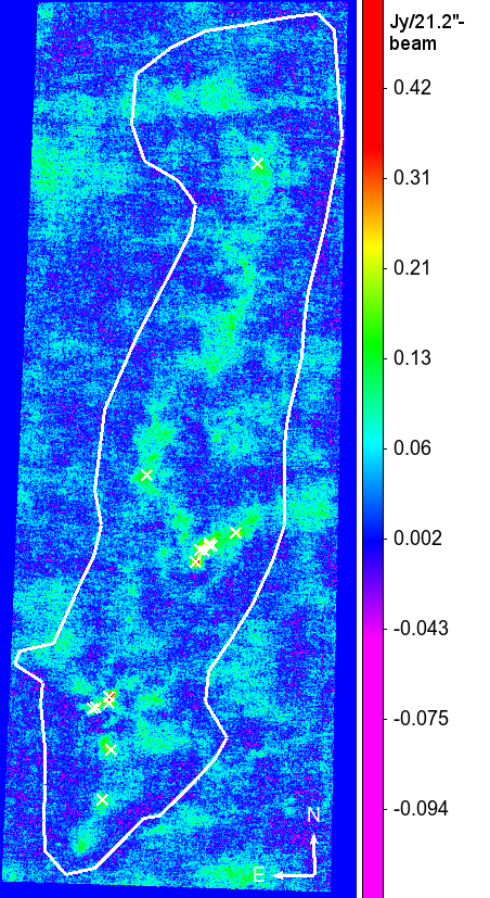
Figure 1: Lupus I LABOCA $870\,\mu$m map with square-root intensity scaling in units of Jy/$21.2\arcsec$-beam. The positions of the 15 cores that were found by Clumpfind are marked with white crosses. The white polygon marks the common area within which the mass of the cloud was calculated from the LABOCA and Herschel column density maps (see Section 4.4).

2.2 Herschel archival data

The Lupus I cloud complex was observed by the Herschel far-infrared observatory (Pilbratt et al. 2010) in January 2011 as part of the Gould-belt survey (André et al. 2010; Rygl et al. 2013). The Photodetector Array Camera and Spectrometer (PACS, Poglitsch et al. 2010) and the Spectral and Photometric Imaging Receiver (SPIRE, Griffin et al. 2010) were used to map an area of $\approx 2\degr\times 2.3\degr$. We retrieved these data from the Herschel science archive and reduced them using HIPE v12.1 (Ott 2010) for the calibration and the deglitching of the Level 0 PACS and SPIRE data. The Level 1 data of both instruments were then used to produce the final maps with the Scanamorphos package v24 (Roussel 2013, /parallel and /galactic options were switched on in both cases to preserve extended structures in complex, bright Galactic fields). The pixel-sizes for the five maps at 70, 160, 250, 350 and 500 $\mu$m were chosen as $3.2\arcsec$, $4.5\arcsec$, $6\arcsec$, $8\arcsec$, and $11.5\arcsec$, respectively.

The absolute calibration of the Herschel data was done following the approach described in Bernard et al. (2010). Using the Planck and the IRAS data of the same field as the Herschel data one calculates the expected fluxes to be observed by Herschel at each band and from that computes the zero-level offsets (see Table 1). Those are then added to the Herschel maps to create the final mosaics.

Table 1: Zero-level offsets for the Herschel maps obtained from the cross-correlation with Planck and IRAS.

Band	Offset
$[\,\mu{\rm m}]$	MJy $\rm sr^{-1}$
70	5.68954
160	14.3011
250	8.11490
350	4.06405
500	1.68754

For the dust properties and temperatures considered in our analysis the color corrections for both PACS and SPIRE are of order 1-2% and hence negligible.

2.3 Planck archival data

We retrieved the all-sky maps of the High-Frequency-Receiver (HFI) in the 353, 545, and 857 GHz bands (corresponding to the FIR and sub-mm wavelengths of 850, 550, and $350\,\mu$m) from the Planck legacy archive (release PR1 21.03.2013). From these data cubes in HEALPix format we extracted for each wavelength separately the area covering the Lupus I region and created gnomonic projected maps. The resolution in each of the three bands is $5\arcmin$ and the pixel size was chosen as $1.7\arcmin$.

3 Data analysis

3.1 Column density and temperature maps of Lupus I

From our three data sets of LABOCA, Herschel, and Planck we calculated column density maps to characterize the cloud in a multi-wavelength approach. Additionally, we constructed a temperature map from the Herschel data.

3.1.1 Column density and temperature map from Herschel SED fit with all SPIRE bands

The standard and often practiced way to derive column density and temperature maps from the Herschel data is to fit an SED to the observed fluxes of the Herschel bands for each pixel of the maps (see e.g. Alves de Oliveira et al. 2014; Lombardi et al. 2014; Battersby et al. 2014). Here we fit the SED to the three SPIRE bands 250, 350, and $500\,\mu$m. We do not include the two PACS 70 and $160\,\mu$m bands, because those observations were corrupted by stray moonlight and hence are not reliable for an analysis of large-scale structures.

Because Lupus I is optically thin to the dust emission at the considered densities and wavelengths we can model its emission as a modified black body. We assume that the long wavelength emission ($\lambda\geq 250\,\mu$m) of a pixel [i, j] comes from a unique species of grains being all at the same equilibrium temperature, and having a power-law wavelength dependent opacity. If $L_{\nu}^{i,j}(\lambda)$ is the monochromatic luminosity of pixel [i, j] at wavelength $\lambda$, then it can be expressed as

$$L^{i,j}_{\nu}(\lambda)=M^{i,j}_{\mathrm{d}}\times\kappa(\lambda_{0})\left(\frac{\lambda_{0}}{\lambda}\right)^{\beta}\times 4\pi\,B_{\nu}(\lambda,T^{i,j}_{\mathrm{d}})$$ (1)

where $\kappa$ is the dust opacity, $\beta$ the emissivity index, $B_{\nu}(\lambda,T_{\mathrm{d}})$ the black body spectral flux density for a dust temperature $T_{\mathrm{d}}$. The two free parameters $M^{i,j}_{\mathrm{d}}$ and $T^{i,j}_{\mathrm{d}}$ are the dust mass and temperature per pixel of the material along the line-of-sight. Here we adopt a typical $\kappa(\lambda_{0})=5.91\,{\rm cm^{2}\,g^{-1}}$ with $\lambda_{0}=350\,\mu$m for dust grains with thin ice mantels and gas densities $<10^{5}$ cm^-3 (Ossenkopf & Henning 1994). Using the available information about $\beta$ from the Planck data, we found that the emissivity index within the Lupus I cloud lies between $\sim 1.6$ and $\sim 1.7$. Therefore we fixed its value to $\beta=1.65$ as an average value within the cloud. Considering the low resolution of the $\beta$ map of $30\arcmin$ this is a reasonable approximation. In this way we also limit the number of free parameters in the fit making it more stable.

After convolving the 250 and $350\,\mu$m maps to the resolution of the $500\,\mu$m band using the kernels from Aniano et al. (2011), the modified black body fit was performed pixel-by-pixel. From the dust mass $M^{i,j}_{\mathrm{d}}$ in each pixel the total column density for both dust and gas was then calculated as

$$N^{\mathrm{H_{SED}}}_{\mathrm{H_{2}}}=\frac{M_{i,j}\,R}{\mu_{\mathrm{H_{2}}}\,m_{H}}$$ (2)

where $R=100$ is the gas-to-dust mass ratio, $\mu_{\mathrm{H_{2}}}=2.8$ the molecular weight per hydrogen molecule, and $m_{\mathrm{H}}$ the hydrogen atom mass. The resulting dust temperature values $T^{i,j}_{\mathrm{d}}$ from the fit at each pixel give the temperature map of Lupus I (shown in Fig. 2) at the resolution of the $500\,\mu$m band, i.e. $\rm FWHM_{500}=36\arcsec$.

Since the composition of the dust grains and their density is unknown, the choice of a particular dust model and thus a specific opacity law introduces an uncertainty of the dust opacity and thus of the resulting column density. In order to estimate it, we took different $\kappa(\lambda_{0})$ values at $350\,\mu$m for grains with and without ice mantles and the three initial gas densities of $<10^{5}$, $10^{5}$, and $10^{6}$ cm^-3 in the online table of Ossenkopf & Henning (1994). They vary between $3.64\,{\rm cm^{2}\,g^{-1}}$ (MRN without ice mantles and $\rho<10^{5}$ cm^-3) and $11.3\,{\rm cm^{2}\,g^{-1}}$ (MRN with thin ice mantles and $\rho=10^{6}$ cm^-3). Hence, our chosen value of $\kappa(\lambda_{0})$ might still vary by a factor of about 2.

The statistical error on both the final column density map and the temperature map consists of errors of the calibration, the photometry, and the SED fitting process. We conservatively estimated the sum of these uncertainties to be $\sim 20\%$ for both maps.

Figure 2: Left: Temperature map of Lupus I from the Herschel SPIRE SED fit. Right: Histogram of the dust temperature for the whole cloud (purple), the northern (orange), and the center-south part (green).

3.1.2 Column density map from Herschel SPIRE $250\,\mu$m map

To obtain a column density map with the resolution of the SPIRE $250\,\mu$m band (i.e. $\rm FWHM_{250}=18\arcsec$), we followed the technique described in Juvela et al. (2013). Using the intensity map of the SPIRE $250\,\mu$m band and the previously calculated temperature map (at the lower resolution) to compute the Planck function $B_{\nu}(T_{\mathrm{d}})$, it is possible to gain another factor of two in resolution compared to the SED fitting (to all three SPIRE bands) case. In this way the column density simply is

$$N^{\mathrm{H_{250}}}_{\mathrm{H_{2}}}=\frac{I_{250\,\mu{\rm m}}^{i,j}\,R}{B_{\nu}(250\,\mu{\rm m},T_{\mathrm{d}}^{i,j})\,\kappa_{250\,\mu{\rm m}}\,\mu_{\mathrm{H_{2}}}\,m_{H}}$$ (3)

with $I_{250\,\mu{\rm m}}^{i,j}$ the intensity of the SPIRE $250\,\mu$m band. We used this higher resolution Herschel column density map for our further analysis of Lupus I.

3.1.3 Column density map from the LABOCA data

Lupus I is sufficiently far away from ionizing UV sources to exclude significant amounts of free-free emission. We may therefore assume the sub-mm fluxes to be entirely due to thermal dust emission. To determine whether the cloud is optically thin in this wavelength regime one can look at the peak intensity in the LABOCA map, which is $I^{\rm max}_{\nu}=1.37$ Jy/beam. The corresponding optical depth can be calculated via formula (3) of Schuller et al. (2009).

$$\tau_{870\,\mu\mathrm{m}}=-\ln\left[1-\frac{I_{\nu}}{\Omega\,B_{\nu}(T_{\mathrm{d}})}\right]$$ (4)

where $\Omega$ is the beam solid angle. In the case of Lupus I this yields values of $\tau_{870\,\mu{\rm m}}\leq 0.01$ for temperatures $T_{\mathrm{d}}\geq 10$ K. Hence the cloud is clearly optically thin in this wavelength regime. Therefore, the $870\,\mu$m intensities are directly proportional to the column densities of the interstellar dust and the line-of-sight extinction. They can be converted to the beam-averaged hydrogen molecule column density via equation (3).

We again assume a gas-to-dust mass ratio of $R=100$ and for consistency extrapolate our dust model used for the Herschel analysis to the LABOCA wavelength, which yields a value of $\kappa_{870\,\mu{\rm m}}=1.32\,{\rm cm}^{2}\,{\rm g}^{-1}$. Because the assumption of a constant dust temperature throughout the cloud is not valid, we used the temperature map from the Herschel analysis to calculate the black body function at each pixel of the map. In this way one obtains a column density map at the original resolution of the LABOCA map (i.e. $\rm FWHM_{870}=21.2\arcsec$).

3.1.4 Column density and temperature map from the Planck data

The thermal emission of interstellar dust over the whole sky was captured by the HFI-instrument of Planck at its 6 available wavelengths between $350\,\mu$m and 3 mm. Together with the IRAS $100\,\mu$m data the emission can be well modeled by a modified black body. The details of the model and the fitting procedure are described in Planck Collaboration et al. (2014). The resulting maps of temperature and optical depth (at $850\,\mu$m) can be downloaded from the Planck archive. We extracted the part covering Lupus I from both maps to get gnomonic projected maps. The column density map was then computed from the optical depth map using the relation

$$N_{\mathrm{H_{2}}}=\frac{5.8\times 10^{21}\,{\rm cm^{-2}}}{2}\times 0.497\times 10^{4}\,\tau_{\rm 353\,GHz}$$ (5)

suggested in Planck Collaboration et al. (2014) for regions with higher column density than the diffuse ISM, i.e. molecular clouds.

3.2 Column density PDFs

Probability distribution functions (PDFs hereafter) of the column density are a widely used way to characterize the evolution and state of molecular clouds. Both simulators (see e.g. Federrath & Klessen 2012; Ward et al. 2014; Girichidis et al. 2014) and observers (see e.g. Kainulainen et al. 2009, 2011; Palmeirim et al. 2013; Tremblin et al. 2014; Schneider et al. 2015; Roccatagliata et al. 2015) use them in their studies and they are a good tool to compare both simulations and observations with each other.

As Lupus I is at near distance to us and lies at a high Galactic latitude, far away from the Galactic plane, we expect the contamination of the map by overlaying foreground or background emission to be small. We normalize the PDFs to the dimensionless $\eta=\ln(N_{\mathrm{H_{2}}}/\langle N_{\mathrm{H_{2}}}\rangle)$ which gives the opportunity to compare different regions of different column density, as well as the same cloud, but observed with different instruments. For similar observations of the Orion clouds Schneider et al. (2013) showed that the effect of varying the resolution of the maps within $18\arcsec$ and $36\arcsec$ did not affect the main features of the PDFs (shape, width, etc.) significantly. The Lupus I cloud is much closer, yielding a much finer physical resolution and the tests we performed on our maps smoothing them with a grid of Gaussians with different FWHM and rebinning them to several different pixel sizes confirmed their findings. If the difference, however, is as big as e.g. the one in angular resolution between Herschel and Planck, it is not longer possible to maintain the features of the PDF unchanged when degrading the Herschel map by a factor of $\approx 8$ (from $500\,\mu$m) to $\approx 17$ (from $250\,\mu$m). But in our case both the angular resolution and the pixel size of the Herschel and the LABOCA column density map are almost the same. Therefore, both maps have sufficiently large numbers of pixels to have a high statistic.

The basic shape of the PDF in the low column density regime can be described by a lognormal distribution. In more complicated cases the PDF might also be the combination of two lognormals:

$$p(\eta)=\frac{\epsilon_{1}}{\sqrt{2\pi\sigma_{1}^{2}}}\exp\left(\frac{-(\eta-\mu_{1})^{2}}{2\sigma_{1}^{2}}\right)+\frac{\epsilon_{2}}{\sqrt{2\pi\sigma_{2}^{2}}}\exp\left(\frac{-(\eta-\mu_{2})^{2}}{2\sigma_{2}^{2}}\right)$$ (6)

where $\epsilon_{i}$ is the norm, $\mu_{i}$ and $\sigma_{i}$ are the mean logarithmic column density and dispersion of each lognormal. In the high column density regime one often finds a deviation from the lognormal. This can be modeled with a power-law of slope $s$ which is equivalent to the slope of a spherical density profile $\rho(r)\propto r^{-\alpha}$ with $\alpha=-2/s+1$ (see Federrath & Klessen 2013; Schneider et al. 2013).

Using a least-square method (Levenberg Marquardt algorithm; Poisson weighting) we derived the characteristic values of the distributions by fitting the PDFs with either one lognormal to the distribution around the single peak and where applicable a power-law to the high density tail, or with two lognormals to the distributions around the first and second peak, respectively, and a possible power-law tail. We checked the robustness of the fits by performing it on four different binsizes for the histograms (0.05, 0.1, 0.15, 0.2) and looking at the variation of the resulting fit parameters which was of the order $2\%-8\%$. We took the final parameters from the fits for a binsize of 0.1 (see Schneider et al. 2015) and conservatively adopted an error of 10% for all fit parameters. The results are summarized in Table 2.

Table 2: Results of the fits to the Herschel PDFs of Fig. 5.

Region	$\sigma_{1}$	$\rm N_{{H_{2}},peak1}$	$\sigma_{2}$	$\rm N_{{H_{2}},peak2}$	$<\rm N_{\mathrm{H_{2}}}>$	$\rm N_{H_{2},dev}$	s	$\alpha$
		[$\times 10^{21}\,{\rm cm^{-2}}$]		[$\times 10^{21}\,{\rm cm^{-2}}$]	[$\times 10^{21}\,{\rm cm^{-2}}$]	[$\times 10^{21}\,{\rm cm^{-2}}$]
Whole cloud	0.56	0.866	0.26	2.57	1.44	3.60	-2.55	1.78
Center-south	0.46	0.934	0.35	2.71	1.72	4.50	-2.43	1.82
north	0.55	0.794	0.18	2.23	1.10	–	–	–

4 Results

4.1 Column density and temperature maps

Figure 3: Column density maps of Lupus I from (a) the Herschel $250\,\mu$m map, (b) LABOCA, and (c) Planck.

The Herschel column density map of Lupus I is shown in Fig. 3. The average column density is ¡$\rm N_{\mathrm{H_{2}}}$¿ $\rm=1.44\times 10^{21}\,cm^{-2}$. The map reveals two distinct regions within the filament (see also Fig. 4). The north where the column densities are lowest (¡$\rm N_{\mathrm{H_{2}}}$¿ $\rm=1.10\times 10^{21}\,cm^{-2}$) and just one dense core can be seen (Rygl et al. 2013) and the center-south part where several cores with high column densities above $\rm 10^{22}\,cm^{-2}$ are found and the average column density (¡$\rm N_{\mathrm{H_{2}}}$¿ $\rm=1.72\times 10^{21}\,cm^{-2}$) is about 60% higher than in the northern part.

Comparing our map to the one derived by Rygl et al. (2013) we note that our values are lower by a factor of about $2-2.5$. This can be explained by the use of a different dust model (opacity and dust spectral index) and the inclusion of the PACS $160\,\mu$m band in their work. The extinction maps created from 2MASS and Spitzer data (see Chapman et al. 2007; Lombardi et al. 2008; Merín et al. 2008) have a resolution that is lower by a factor of $\sim 7-30$. Nevertheless, between those maps and our column density map is a clear resemblance.

The column density map of Lupus I we obtained from LABOCA (see Fig. 3) is dominated by the dozen cores in the center-south part and the denser dust in the central part of the filament. The average column density is ¡$\rm N_{\mathrm{H_{2}}}$¿ $\rm=1.47\times 10^{21}\,cm^{-2}$.

The Planck column density map of Lupus I with a resolution of $5\arcmin$ reveals the basic structure of the cloud which agrees well with the column density maps from LABOCA and Herschel. This is consistent with what is shown by the other two maps when smoothed to the resolution of Planck and thus smoothing out the highest column density peaks.

The temperature map obtained from the Herschel SED fit (see Fig. 2) shows an anti-correlation of the temperature with the column density. The densest parts are the coldest and the less dense the material the warmer it becomes. Also one sees again a difference between the northern and the center-south part of the cloud. In the north dust temperatures between $\approx 15-23$ K with a mean and median of $\approx 19$ K are found. But only in the dense pre-stellar core and slightly north of it the temperature drops down to $\approx 15$ K. The maximum temperature in the center-south part is $\approx 22$ K at the edges of the filament. The inner part of the filament has an average temperature of $\approx 17$ K. But it drops down to even 11 K in the densest cores. From the histogram of the dust temperatures (see Fig. 2) one can see that most of the dust in the north (orange histogram) ranges between $\approx 18-20$ K whereas in the center-south part (green) it is between $\approx 16-18$ K. This means that the dust in the center-south is on average 2 K colder than in the north.

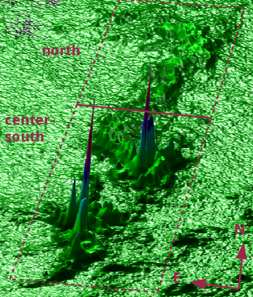
Figure 4: 3D-surface plot of the Herschel $250\,\mu$m column density map. One can clearly identify the cores in the center-south of Lupus I and see the on average lower column density in the northern part of the cloud. The red dashed boxes mark the two regions we distinguish in this work.

4.2 Column density PDFs

We derived PDFs of the Lupus I cloud from the Herschel and LABOCA column density maps for the two distinct parts of the cloud (north and center-south; see Fig. 4), as well as for the whole cloud. They are shown in Fig. 5. For a correct interpretation of the PDFs one has to consider the completeness limit of the underlying column density map. Here we adopted the lowest closed contour as such a limit which is $1.1\times 10^{21}$ and $2\times 10^{21}\,{\rm cm^{-2}}$ for the Herschel and LABOCA map, respectively. It is marked by the vertical dashed line in the plots of Fig. 5.

Looking at the entire cloud the Herschel PDF is very complex with clear deviations from a simple lognormal distribution which would be expected for a cloud that is dominated by isothermal, hydrodynamic turbulence (e.g. Klessen et al. 2000). The distribution shows two peaks in the low column density regime and a power-law tail in the high density end. The first peak at $\rm N_{{H_{2}},peak1}=8.66\times 10^{20}\,{\rm cm^{-2}}$ falls below our completeness limit, so it might be just reflecting the drop of observational sensitivity and will not be used for interpretation. But the distribution above the limit can be well represented by a fit of two lognormals around the first and second peak which is at $\rm N_{{H_{2}},peak2}=2.57\times 10^{21}\,{\rm cm^{-2}}$. The width of the first component is $\sigma_{1}=0.56$, but could also be broader due to the possible underestimate of the column densities below the completeness limit. Nevertheless, it is more than twice as broad as the width of the second lognormal ($\sigma_{2}=0.26$) and larger than in other nearby clouds like Maddalena, Auriga (Schneider et al. 2013) or Aquila (Schneider et al. 2015). This can be a sign of broadening by turbulence and external compressive forcing (see Federrath et al. 2010; Tremblin et al. 2012; Federrath & Klessen 2013). The power-law tail follows a slope of $\rm s=-2.55$ or corresponding $\alpha=1.78$ for a spherical density distribution. The deviation from the lognormal into the power-law occurs near $\rm N_{{H_{2}},dev}=3.6\times 10^{21}\,{\rm cm^{-2}}$ which is slightly below the recent values by Schneider et al. (2015) who found the transition into the power-law tail to be at $A_{V}\sim 4-5$ mag in their investigation of four low-mass and high-mass star forming regions. But it is higher than the result of Roccatagliata et al. (2015) who find the deviation to occur at $A_{V}\sim 1.2-2$ mag in the Serpens Core region.

From the Herschel data the center-south part of the cloud shows a PDF very similar to that of the entire cloud. Here again two peaks are present and the distribution above the completeness limit can be fitted by a double lognormal and a power-law tail. The width of the first fitted lognormal is narrower, the width of the second broader than those of the entire cloud with values of $\sigma_{1}=0.46$ and $\sigma_{2}=0.35$. The slope of the power-law is slightly flatter with $\rm s=-2.43$, but leading to a comparable exponent $\alpha=1.82$.

Also in the northern part of the cloud the double peak lognormal profile of the PDF from Herschel is found again. But now there is no excess above the second lognormal at higher densities. The peak position of the first lognormal is lower ($\rm N_{{H_{2}},peak1}=7.94\times 10^{20}\,{\rm cm^{-2}}$) compared to the center-south and the whole cloud, but with similar width ($\sigma_{1}=0.55$). The peak position of the second lognormal ($\rm N_{{H_{2}},peak2}=2.23\times 10^{21}\,{\rm cm^{-2}}$) is lower than that of the whole cloud and its width ($\sigma_{2}=0.18$) is approximately half as broad.

Although it is not possible to strictly constrain the shape of the PDF below the completeness limit, one can say that the distribution above shows not just two components (lognormal and a power-law) but at least three because of the second peak that appears before the deviation into the power-law. Such a shape could be attributed to an initial turbulent cloud which later was compressed by an external driving agent. Such an agent can either be an ionization front, an expanding shell driven by winds or/and supernovae or colliding flows. The initial lognormal form of the PDF of the cloud develops a second component caused by the dense compressed gas. This behavior was found in simulations by Tremblin et al. (2012) of an initial turbulent medium that is ionized and heated by an ionization source. They concluded that a double peak is present when the ionized gas pressure dominates over the turbulent ram pressure of the cloud. Matsumoto et al. (2015) studied the evolution of turbulent molecular clouds swept by a colliding flow. They found that the PDF exhibits two peaks in the case when the Mach numbers of the initial turbulence and the colliding flow are of the same order $M=10$ (model HT10F10; see their Fig. 11b) and the line of sight is perpendicular to the colliding flow. Then the low column density peak represents the colliding flow and the higher column density peak the sheet cloud, respectively. Observationally, double peak PDFs have been reported and studied recently by Schneider et al. (2012), Harvey et al. (2013), and Tremblin et al. (2014) for several nearby clouds exposed to an ionization source. Areas of the cloud close to the ionization front indeed showed the predicted second peak in the PDF due to the compression induced by the expansion of the ionized gas into the molecular cloud. In the case of Lupus I the source of the compression is very likely the expanding H I shell around the USco sub-group of Sco-Cen (possibly together with a supernova that exploded within USco) and the wind bubble of the remaining B-stars of UCL pushing from the eastern and western side of the cloud, respectively. This scenario will be discussed in more detail in Sec. 5.

Lognormal PDFs indicate shock waves (Kevlahan & Pudritz 2009) or turbulence (e.g. Vazquez-Semadeni 1994; Federrath et al. 2010). Tremblin et al. (2012) have shown in a simulation of Stroemgren spheres advancing into turbulent regions that the region compressed by the ionization front also has a lognormal density PDF, but shifted to higher density due to the compression. A PDF of a region that includes compressed and undisturbed parts of the cloud will thus show a double peak PDF.

The power-law tail that is seen in our PDFs could be explained by active star formation and the transition to a gravity dominated density regime represented by the star forming cores. This can be shown by comparing the PDFs of the two regions in the north and the center-south. In the north where there is almost no star formation and just one pre-stellar core and $\approx 20$ unbound cores can be found (Rygl et al. 2013), the PDF shows no power-law tail in the high density regime. In the center-south instead where almost all the star formation activity takes place with plenty of very young bound cores, the PDF shows the power-law tail very clearly. Also numerical studies have shown that the PDF for an actively star forming region develops a clear deviation from the lognormal in form of a power-law tail (Ballesteros-Paredes et al. 2011; Girichidis et al. 2014).

With LABOCA the PDF of Lupus I can be modeled as one lognormal with a power-law tail at high densities ($\rm N_{{H_{2}},dev}=6.0\times 10^{21}\,{\rm cm^{-2}}$). The peak of the lognormal distribution lies at $\rm N_{{H_{2}},peak}=1.43\times 10^{21}\,{\rm cm^{-2}}$ which is below the completeness limit of the LABOCA column density map. The width of the lognormal is broad ($\sigma=0.56$), but uncertain due to the peak position and thus possibly even broader. The power-law slope ($s=-2.66$, $\alpha=1.75$) is very similar to the one of the Herschel PDF indicating the star formation activity in the cloud.

The PDF of the center-south region shows the same behavior as the one for the whole cloud. The lognormal part is slightly broader ($\sigma=0.60$), but the power-law slope ($s=-2.59$, $\alpha=1.77$) and the deviation point ($6.0\times 10^{21}\,{\rm cm^{-2}}$) are almost the same compared to the whole cloud. In the northern part only the now narrower lognormal is seen instead ($\sigma=0.52$), indicating the lack of star formation activity and the dominance by the turbulence induced trough the compression. In all three cases the positions of the peak are very close to each other.

As was already seen in the column density map from LABOCA, its PDF shows only the dense cores and the intercore medium. The instrument is not sensitive to all material that can still be probed with Herschel. With LABOCA we thus sample more the second lognormal of the Herschel PDF and the power-law tail.

Figure 5: Column density PDFs of Lupus I and their model fits for the north and the center-south part of the cloud, as well as for the entire cloud. The error bars show the $\sqrt{N}$ uncertainties. In case of Herschel the two yellow and purple dashed lines show the fits of the two lognormals to the distribution around the first and second peak, respectively. Their superposition is represented by the solid green line. For LABOCA the solid green line shows the lognormal fit to the distribution around the peak. For all cases the straight solid red line shows the power-law fit to the high-density tail of the PDF, if applicable. In each plot we give the value of the dispersion(s) of the fitted lognormal(s) $\sigma_{i}$, the position(s) of the peak(s) of the lognormal(s) $\rm N_{{H_{2}},peak_{i}}$, the slope of the fitted power-law tail s, the corresponding slope of an equivalent spherical density distribution $\alpha$, the mean column density ¡$\rm N_{\mathrm{H_{2}}}$¿, and the deviation point from the lognormal to the power-law tail $\rm N_{{H_{2}},dev}$. The vertical dashed line marks the incompleteness limit (lowest closed contour) which is $1.1\times 10^{21}$ and $2\times 10^{21}\,{\rm cm^{-2}}$ for the Herschel and LABOCA map, respectively.

4.3 Core distribution

For the core analysis in the LABOCA map we used the Clumpfind package (Williams et al. 1994). It decomposes the emission of the map into a set of clumps or cores contouring the data at given threshold levels. The results can be found in Tab. 3 and the distribution of the cores (represented by the white crosses) is shown in Fig. 1. The algorithm identified 15 different cores with masses between 0.07 and $1.71\,M_{\odot}$. Their total mass is $8.37\,M_{\odot}$ and their total flux is 25.39 Jy. This corresponds to $\approx 5\%$ of the total mass of Lupus I (see Sec. 4.4) and $\approx 5\%$ of the total flux of the LABOCA map, respectively. For the computation of the core masses, we derived their temperatures from the Herschel SPIRE SED fit temperature map as a mean temperature within the ellipse representing the core. With this temperature the mass of the cores was calculated following Schuller et al. (2009)

$$M=\frac{d^{2}F_{\nu}R}{B_{\nu}(T_{\mathrm{d}})\kappa_{\nu}}$$ (7)

where $d$ is the distance to Lupus I, $F_{\nu}$ the total flux of the core, $R=100$ the dust-to-gas ratio, and $\kappa_{\nu}=1.32\,{\rm cm}^{2}\,{\rm g}^{-1}$ (see Sec. 3.1.3). Most interestingly, all but one core are found in the center-south part of Lupus I. This confirms our interpretation of the column density maps that is the part where active star formation is going.

The distribution of the cores from the Herschel data (Rygl et al. 2013) agrees with this picture and the core distribution from our LABOCA map. The northern part of Lupus I is mainly populated by unbound cores and just one pre-stellar core wheras the center-south is dominated by pre-stellar cores. Many of those coincide with our LABOCA cores. However, a direct assignment is not easily possible since the Herschel coordinates can only be estimated from the source images in the paper of Rygl et al. (2013) and in some cases several Herschel sources seem to be on the position of one LABOCA source or vice-versa.

Benedettini et al. (2012) found eight dense cores in Lupus I using high-density molecular tracers at 3 and 12 mm with the Mopra telescope (red diamonds in Figure 6). Seven of those have one or more counterparts in our LABOCA map. The matches are given in Table 3. They classify five of their cores as very young protostars or pre-stellar cores (Lup1 C1-C3, C5, and C8) and the remaining three also as very likely to be protostellar or pre-stellar. For three of their cores (Lup1 C4, C6, and C7) they calculated a kinetic temperature of $\approx 12$ K. This agrees within 20% with the core temperatures derived from the Herschel SPIRE SED fit temperature map.

From the 17 young stellar objects found in Lupus I by the Spitzer c2d near-infrared survey (Chapman et al. 2007; Merín et al. 2008) 11 lie within the boundaries of the LABOCA map (blue boxes in Figure 6). But only one object (IRAS 15398–3359) clearly matches one of our LABOCA cores (#1). This is the long known low-mass class 0 protostar IRAS 15398–3359 (inside the B228 core) which has a molecular outflow (see recently e.g. Oya et al. 2014; Dunham et al. 2014). Two other objects of the c2d survey are close, but offset by $\approx 0.5\arcmin$ to the center of our cores #3 and #5, respectively. Nevertheless, each of those two objects still lies within the boundaries of the corresponding ellipse representing the LABOCA core (see Table 3). Most of the LABOCA cores are potentially at a very early evolutionary stage, i.e. without a protostar inside to heat it and eventually destroy the surrounding dust envelope to allow near-infrared radiation to escape. In fact the only cores with a $70\,\mu$m counterpart, which is a good proxy for a protostar inside a core, are number #1 and #3. Therefore, we do not expect to find many Spitzer counterparts.

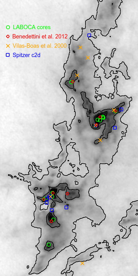
Figure 6: Herschel column density map of the center-south region with contour levels of 1.1, 4, 7, and $10\times 10^{21}\,{\rm cm^{-2}}$. The different symbols mark the center positions of the cores found with LABOCA and of objects found in other studies as discussed in Section 4.3.

Vilas-Boas et al. (2000) found 15 (14) condensations in $\rm C^{18}O$ ($\rm{}^{13}CO$) with the 15 m SEST telescope. Eight cores lie within our LABOCA map (orange crosses in Figure 6) and of those three (Lu7, Lu10, B228) coincide with LABOCA detected cores (#12, #5, and #1). Their $\rm C^{18}O$ excitation temperatures are 9, 11, and 10 K, respectively. This is $\approx 20-40\%$ lower than the temperatures from the Herschel map. For cores Lu7 and Lu10 they calculated a mass from $\rm C^{18}O$ of 11.7 and 3.1 $M_{\odot}$, respectively. This is a factor of $\approx 20$ and $\approx 7$ higher than the LABOCA masses. But the sizes of their condensations were on average larger than at least three times their beam size of $48\arcsec$.

Figure 6 shows the Herschel column density map of the center-south region with contour levels of 1.1, 4, 7, and $10\times 10^{21}\,{\rm cm^{-2}}$. Overploted are the LABOCA cores found in this study (green circles), as well as the above mentioned cores and YSOs found by Benedettini et al. (2012) (red diamonds), Vilas-Boas et al. (2000) (orange crosses), and the Spitzer c2d survey (blue boxes), respectively.

Our findings confirm that Lupus I harbors a population of very young cores that are forming stars just now and probably have ages below 1 Myr. This could support the idea of an external shock agent, like the USco shell, sweaping up the cloud and triggering the simultaneous formation of new stars within the cloud.

Table 3: Parameters of the 15 cores detected in the LABOCA map with Clumpfind (see Fig. 1). The beam size (HPBW) and area used to convert intensities into fluxes is $21.2\arcsec$ and $509\leavevmode\nobreak\ {\rm arcsec^{2}}$, respectively. The total mass of all cores is $\approx 8\,M_{\odot}$. The 4th and 5th column give the FWHM of the ellipses representing the cores. The 6th, 7th, and 8th column give the core’s peak intensity, total flux, and mass, respectively. The core temperature shown in the 9th column was derived from the Herschel SPIRE SED fit temperature map as a mean temperature within the ellipse representing the core. The last column gives the matches to dense cores found by Benedettini et al. (2012).

#	Ra	Dec	FWHMx	FWHMy	Imax	Ftot	Mcore	Tcore	Counterpart
			$[\arcsec]$	$[\arcsec]$	[Jy/beam]	[Jy]	[M⊙]	[K]
1	15:43:01.68	$-$34:09:08.9	58.22	44.38	1.37	5.61	1.71	14.0	Lup1 C4
2	15:44:59.85	$-$34:17:08.8	62.51	44.09	0.51	3.97	1.59	12.0	Lup1 C6
3	15:45:13.58	$-$34:17:08.8	46.56	33.45	0.33	1.48	0.40	15.0	Lup1 C7
4	15:45:16.02	$-$34:16:56.6	35.31	34.95	0.31	1.00	0.27	15.0	Lup1 C7
5	15:45:03.80	$-$34:17:57.3	57.22	42.24	0.28	1.41	0.46	13.5	Lup1 C6
6	15:42:52.86	$-$34:08:02.1	96.42	49.94	0.28	3.85	1.34	13.0	Lup1 C3
7	15:42:43.57	$-$34:08:14.2	70.62	44.38	0.25	1.64	0.57	13.0	Lup1 C3
8	15:42:44.55	$-$34:08:32.5	30.55	20.85	0.25	0.48	0.17	13.0	Lup1 C3
9	15:42:44.06	$-$34:08:44.6	36.82	19.26	0.24	0.49	0.17	13.0	Lup1 C3
10	15:42:50.42	$-$34:08:38.5	53.28	30.34	0.22	1.05	0.36	13.0	Lup1 C3
11	15:45:25.10	$-$34:24:01.8	42.46	69.57	0.22	1.63	0.53	13.5	Lup1 C8
12	15:42:23.02	$-$34:09:33.2	68.97	46.08	0.21	1.72	0.53	14.0	Lup1 C1
13	15:39:09.92	$-$33:25:30.9	27.24	27.70	0.20	0.34	0.07	17.0	–
14	15:45:55.75	$-$34:29:23.7	28.10	26.28	0.20	0.29	0.08	14.5	–
15	15:42:47.90	$-$33:53:15.3	43.80	19.59	0.19	0.43	0.12	15.0	Lup1 C2

4.4 Total mass estimates of Lupus I

To derive the total mass of the cloud from the three different column density maps we defined a polygon around the filament (delineated in Fig. 1 on the LABOCA map) to derive the total mass always in the same area ($\rm\approx 1\,deg^{2}$). The total gas and dust mass was then calculated via the formula

$$\rm M^{\rm tot}_{Lupus\leavevmode\nobreak\ {\rm I}}=\sum\,N_{\mathrm{H_{2}}}\,\mu_{\mathrm{H_{2}}}\,m_{H}\,A_{p}$$ (8)

with $A_{p}$ the area of a pixel in $\rm cm^{2}$. As the common lower level we chose $\rm N_{\mathrm{H_{2}}}>10^{21}\,cm^{-2}$ which corresponds to $\rm A_{V}>1$ mag. The resulting total mass for Lupus I is $\rm M^{\rm tot}_{Lupus\leavevmode\nobreak\ {\rm I}}\approx 171\,M_{\odot}$, $\approx 174\,M_{\odot}$, and $\approx 164\,M_{\odot}$ for the Planck, Herschel, and LABOCA data. This means that the total masses calculated from the three data sets agree with each other. Comparing the total mass of the cloud to the total mass in cores from LABOCA ($\approx 8\,M_{\odot}$) one sees that only about 5% of the mass is concentrated in the densest condensations. Most of the dust and gas is in more diffuse components.

The most recent literature value for the total mass of Lupus I is from the Herschel data by Rygl et al. (2013). They calculated the total mass in a much bigger area than this work ($\approx 4.5\,{\rm deg}^{2}$ compared to our $\approx 1\,{\rm deg}^{2}$) and used a different method to create their column density map as mentioned already in Sec. 4.1. Therefore, a difference of about a factor $4-5$ arises between their value of $M=830\,M_{\odot}$ (for $A_{V}>2$ mag) and our finding.

Other literature values cover a wide range of total masses for Lupus I, depending on the tracer used and the size of the area that was considered. From the Spitzer c2d near-infrared extinction maps Merín et al. (2008) determined a total mass of $479\,M_{\odot}$ for $A_{V}>3$. Various CO measurements (e.g. Tachihara et al. 1996; Hara et al. 1999; Tothill et al. 2009) yielded values of $\approx 280-880\,M_{\odot}$. Direct comparisons with our values are not always possible since all maps cover different parts of the Lupus I cloud complex and the material is not homogeneously distributed to allow scaling the mass with the area. But we note that our values agree with most of the literature values within a factor of 2-3 which is expected considering the uncertainties in the choice of the dust model, the dust-to-gas ratio and the CO-to-H₂ conversion factors.

5 The surroundings of Lupus I and the interaction with USco and UCL

Best suited for looking at the dust surroundings of Lupus I are the Planck data (see Fig. 7 and Fig. 8). These observations at 350, 550, and $850\,\mu$m cover the whole sky at a resolution of $5\arcmin$. Lupus I lies on the eastern edge (Galactic coordinates) of a ring-like dust ridge (labeled in Fig. 8) that extends from about $b=+10\degr$ to $b=+25\degr$ in Galactic latitude with a center at about $l=+345\degr$, $b=17.5\degr$. The ridge is $\sim 5\degr$ wide which corresponds to $\sim 13$ pc at the distance of Lupus I. Besides Lupus I it consists of several small molecular clouds extending north of Lupus I and then bending towards the east connecting with the $\rho$ Ophiuchus molecular cloud on the opposite site of Lupus I. Further west of Lupus I no dust emission is seen in the Planck maps. The same is true for the inside of the dust ridge. Between $\rho$ Ophiuchus and Lupus I a roundish dust void is seen. However, these two dust voids on either side of Lupus I are filled with hot X-ray gas which can be seen with ROSAT (left in Fig. 7). Fig. 8 shows the dust emission seen by Planck in $350\,\mu$m. Overlayed in white are the contours of the ROSAT diffuse X-ray emission at 3/4 keV. Inside USco the contours follow the edge of the dust ridge indicating that the hot X-ray gas might be in contact with the cold dust. On the western side of Lupus I the contours mark the outline of the second roundish X-ray emission seen in ROSAT. The cyan dots mark the remaining early B-type stars of UCL. Both contours seem to wrap around Lupus I what might be a sign that the cloud is embedded in hot ISM.

These dust voids and the observed X-ray gas might be explained by the cumulative feedback of the massive stars in the USco and UCL sub-groups of Sco-Cen. Their creation has been interpreted in a scenario of propagating molecular cloud formation and triggered cloud collapse and star formation taking place within the last 17 Myr in the UCL and USco sub-groups of Scorpius-Centaurus (see de Geus 1992; Preibisch & Zinnecker 2007). The expansion of the UCL H I shell that started $\sim 10$ Myr ago and was driven by winds of the massive stars and supernovae explosions has probably cleared out almost all the dust and molecular material west of Lupus I. But the observed X-ray gas on that side is probably not related to the supernova explosions, because the X-ray luminosity of supernova-heated superbubbles dims on a timescale of typically less than a million years via expansion losses and mixing with entrained gas (Krause et al. 2014). The shell today has a radius of $\sim 110$ pc (as seen from H I data; de Geus 1992), generally consistent (compare, e.g. Baumgartner & Breitschwerdt 2013; Krause et al. 2013) with the inferred age of the stellar group, about 17 million years. Therefore, this X-ray gas is probably currently heated by the remaining B-stars of UCL. Six of those stars south-west of Lupus I ($325\degr<l<335\degr$ and $10\degr<b<15\degr$; see Fig. 8) lie at positions that favor them as likely being the sources of this wind bubble.

The USco H I shell has started its expansion $\sim 5$ Myr ago powered by the winds of the OB-stars and quite possibly a recent supernova explosion, about 1.5 Myr ago, as suggested by the detection of the 1.8 MeV gamma ray line towards the USco sub-group and the detection of the pulsar PSR J1932+1059 (Diehl et al. 2010, and references therein). What now forms the before mentioned dust ridge is probably the remaining material of the USco parental molecular cloud that was swept up by the advancing USco shell leaving the dust void filled with X-ray gas. From simulations, we expect large scale oscillations of the hot, X-ray emitting gas (Krause et al. 2014), because the energy source is never exactly symmetric.

It seems like the UCL wind bubble could be colliding with the USco H I shell right at the position of Lupus I squeezing it in-between. This wind bubble might have provided a counter-pressure to the expanding USco shell and thus favored this position for an additional compression of the shell material. In this way a new molecular cloud could have been created there and it might explain why we do not see more very young star forming clouds (except $\rho$ Oph) distributed within the wall of the USco shell. With its distance of 150 pc the cloud also is neither in the foreground of the B-stars of UCL that have an average distance of $\sim 140$ pc (de Zeeuw et al. 1999) nor in front of USco ($\sim 145$ pc; Preibisch et al. 2002). To rule out shadow effects completely, however, a more comprehensive analysis of the X-ray data would be required.

From our preliminary analysis of the GASS H I data (McClure-Griffiths et al. 2009; Kalberla et al. 2010) we see that Lupus I is indeed embedded within the expanding shell around USco (Kroell et al., in prep.). The shell has an expansion velocity of $\approx 7\,{\rm km\,s^{-1}}$ and a thickness of $\approx 6$ pc. We estimate the current outer radius to be $\approx 36$ pc (both inner and outer radius of the USco shell from our H I model are delineated in Fig. 7).

These findings complement previous suggestions of an interaction of Lupus I (and $\rho$ Oph) with the two sub-groups of Sco-Cen that were originally proposed by de Geus (1992). From the spatial and velocity structure of $\rm{}^{12}CO$ observations Tachihara et al. (2001) also found evidence for an interaction. Tothill et al. (2009) in their analysis of $\rm{}^{13}CO$ and CO(4-3) found enhanced line widths at the western end of Lupus I and a velocity gradient across the filament, i.e. in the direction of the USco shell expansion, of $\rm\sim 1\,km\,s^{-1}$ which they conclude to be consistent with a dynamical interaction between Lupus I and the USco H I shell. Matthews et al. (2014) have found that the large-scale magnetic field is perpendicular to the Lupus I filament, i.e. points in the direction of the USco shell expansion. This might have favored the accumulation of cold, dense atomic gas along the field lines and promote faster molecule formation (Hartmann et al. 2001; Vázquez-Semadeni et al. 2011).

All these are hints towards the scenario that Lupus I was affected by large-scale external compressing forces coming from the expansion of the USco H I shell and the UCL wind bubble. This might explain its position, orientation and elongated shape, the appearance of a double peak in the PDF and the large population of very young pre-stellar cores that are seen with both LABOCA and Herschel.

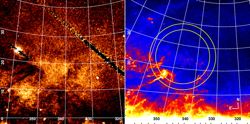
Figure 7: The surrounding of Lupus I in X-rays (ROSAT $3/4$ keV, left) and dust emission (Planck $850\,\mu$m, right). There are two X-ray bubbles on either side of the Lupus I ridge and both Lupus I and $\rho$ Ophiuchus as well as the little cloudlets north of them seen in dust emission have X-ray shadows. The yellow dashed circles in the right image give the position of the inner and outer edge of the USco H I shell determined from our preliminary analysis of the GASS H I data. The center lies at $l=347\degr$, $b=25\degr$ and the inner and outer radius is $12\degr$ and $15\degr$, respectively.

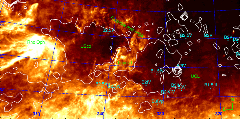
Figure 8: The surroundings of Lupus I seen in dust emission (Planck $350\,\mu$m). The white contours mark the X-ray emission (ROSAT 0.8 keV) from $0.27-1\times 10^{-3}$ counts/s. The cyan dots mark the positions of the B1-B3 stars of UCL from the Hipparcos catalog. Labels are given in green.

6 Summary and Conclusions

From our LABOCA observations of Lupus I as well as from archival Herschel and Planck data we created column density maps of the cloud. In addition we calculated a temperature map from an SED fit using the three SPIRE bands of Herschel. All maps suggest that the cloud can be divided into two distinct regions. The northern part that has on average lower densities and higher temperatures as well as no active star formation and the center-south part with dozens of pre-stellar cores where density and temperature reach their maximum and minimum, respectively.

From the LABOCA and Herschel maps we derived column density PDFs for the entire cloud as well as for the two above mentioned regions separately. The Herschel PDF of Lupus I showed a double peak profile with a power-law tail. The power-law can be attributed to the star formation activity in the center-south part of the cloud since it disappears in the PDF of the northern part. However, the double peak profile is conserved throughout the cloud and possibly arises due to the large-scale compressions from the cumulative massive star feedback of the Sco-Cen sub-groups. Such a sign for compression in the PDF was previously found in both observations and simulations of advancing ionization fronts, also supported by simulations of colliding turbulent flows. With LABOCA we probe the denser parts of Lupus I and find one lognormal and the power-law tail for the whole cloud and the center-south. The PDF of the northern part shows only the lognormal behavior.

The distribution of the 15 cores that were found in our LABOCA map confirms that only the center-south part of Lupus I is actively forming stars whereas the north is quiescent. The cores have masses between 0.07 and $1.71\,M_{\odot}$ and a total mass of $\approx 8\,M_{\odot}$. As the cloud has a total gas and dust mass of $\approx 164\,M_{\odot}$ (from LABOCA for $\rm N_{\mathrm{H_{2}}}>10^{21}\,cm^{-2}$) this means that $\sim 5\%$ of the mass is in cores. All of those cores are pre-stellar or protostellar confirming that we are witnessing a large star formation event (see e.g. Benedettini et al. 2012; Rygl et al. 2013). The total mass from Herschel and Planck for $\rm N_{\mathrm{H_{2}}}>10^{21}\,cm^{-2}$ was $\approx 174\,M_{\odot}$ and $\approx 171\,M_{\odot}$, respectively.

We argue that the main driving agents in the formation process of Lupus I are the advancing USco H I shell, which most likely contains the cloud, and the UCL wind bubble interacting with the USco shell and hence squeezing Lupus I in-between these two shells in a complex manner. The age of the population of young stellar objects suggests a compression event $\sim 1-2$ Myr ago, which could be the interaction between the two shells and possibly a supernova explosion as suggested by the gamma ray data (Diehl et al. 2010). This large-scale compressions might be the reason for the position, orientation and elongated shape of Lupus I, as well as the double peak PDFs and the population of very young pre-stellar cores we found.

In future work we will analyze our newly performed high-resolution APEX CO line observations to study the kinematics of the Lupus I cloud. We will also compare our observational findings with dedicated numerical simulations and search for signs in the theoretical PDF that will allow us to distinguish between different scenarios of molecular cloud formation.