Investigation of Hot X-ray Points (HXPs) Using Spectroheliograph Mg xii Experiment Data From CORONAS-F/SPIRIT

Abstract

Observations in the Mg xii 8.42 Å line onboard the CORONAS-F satellite have revealed compact high temperature objects—hot X-ray points (HXP)—and their major physical parameters were investigated. Time dependencies of temperature, emission measure, intensity, and electron density were measured for 169 HXPs. HXP can be divided into two groups by their temperature variations: those with gradually decreasing temperature and those with rapidly decreasing temperature. HXPs plasma temperatures lie in the range of 5 – 40 MK, the emission measure is $10^{45}$ – $10^{48}$ cm^-3, and the electron density is above $10^{10}$ cm^-3, which exceeds the electron density in the quiet Sun ($10^{8}$ – $10^{9}$ cm^-3). HXPs lifetimes vary between 5 – 100 minutes, significantly longer than the conductive cooling time. This means that throughout a HXP’s lifetime, the energy release process continues, which helps to maintain its high temperature. A HXP’s thermal energy is not greater than $10^{28}$ erg, and the total energy, which is released in HXPs, does not exceed $10^{30}$ erg. HXPs differ in their physical properties from other flare-like microevents, such as microflares, X-ray bright points, and nanoflares.

1 Introduction

The process of plasma heating in the solar corona to temperatures beyond 5 MK occurs due to intense energy release. The study of these processes is important for understanding the reason for energy release, measuring the physical conditions in which these processes take place and for compiling a comprehensive picture of events occurring in the solar corona. Images of hot plasmas have been obtained from X-ray telescopes such as the Yohkoh/SXT [Tsuneta et al. (1991), Ogawara et al. (1991)], the RHESSI [Lin et al. (2002)], XRT/Hinode [Kosugi et al. (2007), Golub et al. (2007)], and the spectroheliograph Mg xii/SPIRIT [Zhitnik et al. (2003a)]. These images showed that hot plasma is not present everywhere in the solar corona, but just in its compact areas. High-temperature events of the solar corona are flares, hot loops, microflares [Lin et al. (1984), Benz and Grigis (2002)], active-region transient brightenings (ARTB: shi95).

Here we present an analysis of 169 compact high-temperature objects (“hot X-ray points”, HXPs) observed between 20 February 2002 and 28 February 2002 using the spectroheliograph Mg xii as part of the CORONAS-F/SPIRIT experiment.

2 Experimental Data

The Mg xii spectroheliograph is a part of the SPIRIT instrumentation complex, developed in the Lebedev Physical Institute of the Russian Academy of Sciences [Zhitnik et al. (2003b)]. The Mg xii spectroheliograph obtains monochromatic images of the solar corona in $\lambda=8.42$ Å. A high degree of monochromaticity is achieved by using an optical scheme with a spherical crystal mirror (see Figure F:Spectroheliograph_Mg_XII), for which Bragg’s law is satisfied for a narrow wavelength band (only the Mg xii 8.42 Å doublet line is detected). Reflection from the surface of the mirror occurs only from its small parts where Bragg’s law is satisfied:

$$\ilabel{E:Breg}2d\cos{\theta}=m\lambda$$ (1)

(interplanar distance $d$ ($2d=8.501$ Å), angle between incident ray and normal to a mirror $\theta$, order of diffraction $m$, wavelength $\lambda$). For a working wavelength of $\lambda=8.42$ Å, Bragg’s angle is close to $90^{\circ}$, and an almost normal incidence occurs. Normal incidence allows us to obtain a high spatial resolution, $\approx 8^{\prime\prime}$ (effective size of the CCD’s pixel is $\approx 6^{\prime\prime}$).

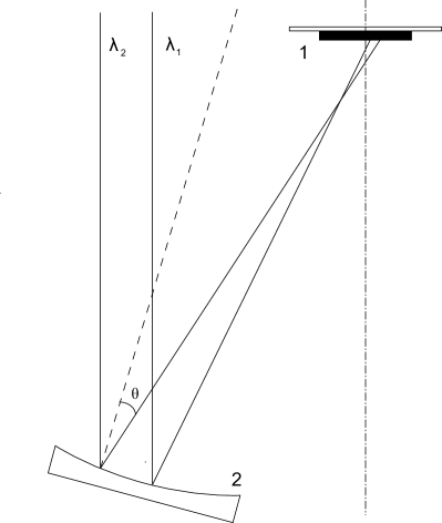
Figure 1.: Scheme of the Mg xii spectroheliograph: 1 - CCD matrix, 2 - spherical crystal mirror.F:Spectroheliograph˙Mg˙XII

Equation (E:Breg) shows that different wavelengths reflect at different angles, and therefore from different parts of the mirror. Due to spherical aberrations of the mirror, rays that have the same incident angle and a different site of reflection will be focused on different parts of the CCD matrix. Thanks to this effect, the Mg xii spectroheliograph has a small dispersion and at the same time can build up 2D images.

Due to spectroheliograph dispersion, images in different components of the Mg xii doublet ($\lambda_{1}=8.4192$ Åand $\lambda_{2}=8.4246$ Å, corresponding to level transitions $1s\ {}^{2}S_{1/2}$ – $2p\ {}^{2}P_{1/2}$ and $1s\ {}^{2}S_{1/2}$ – $2p\ {}^{2}P_{3/2}$) are shifted from one another. The distance between the two doublet components amounts to five pixels (one pixel is 0.00104 Å), while the spectral width of the lines amounts to two pixels. An image of the compact source with a size less than one pixel shows a structure that is elongated in the direction of the dispersion. The transverse width of this structure is defined by a point spread function of the mirror and its FWHM equals $\approx$ one pixel. Its length amounts to 10–15 pixels and is determined by dispersion of the device and the line’s spectral width.

Figure 2.: Contribution function of Mg xii channelF:GOFT

Emission of the Mg xii 8.42 Å line occurs in hot plasma with $T>$ 5 MK (see Figure F:GOFT). That is why images obtained from Mg xii spectroheliograph differ from images in cool lines obtained from other telescopes (for example Yohkoh/SXT): there is no limb visible on these images and they consist of separate localized sources. An example of an image obtained using the Mg xii spectroheliograph is shown on Figure F:compact_structureb. An image obtained from Yohkoh/SXT in 2 – 40 Å spectral band ($T$ $>$ 2 MK) is shown in Figure F:compact_structurea. These two images are taken at close points in time. HXPs are designated with arrows in these figures. Assuming that they are point sources, the transverse sizes of these structures on the Mg xii image are determined by spectroheliograph point spread function, and the elongation is caused by spectral dispersion. Images of the Mg xii spectroheliograph resemble images from the Yohkoh/SXT with Be-filter. HXPs, which are seen on spectroheliograph images, are also seen on Be-filter images.

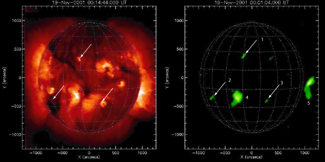
                              (a)                               (b)

Figure 3.: Images taken by Yohkoh/SXT (a) and Mg xii spectroheliograph (b) at close points of time. HXPs are designated by arrows on both images. 1, 2, 3 – HXP; 4, 5 – large hot structures.F:compact˙structure

Observations using the Mg xii spectroheliograph carried out between 20 and 28 February 2002 were used for this analysis. At that time the satellite was in completely illuminated orbits, and the Mg xii spectroheliograph obtained images continuously with cadences from 40 – 120 seconds. A total of 8689 images were taken.

3 Temporal Characteristics

An example of a series of images with evolving HXP is shown in Figure F:light_curve. On the same image, temporal variations of the intensity (light curve) is also shown. In addition, the times of registration of separate images are marked with arrows. Here, we understand “intensity of a source” as a flux from this source in a given spectral band at the Earth’s orbit. No ground-based calibration of the sensitivity of the spectroheliograph was carried out, which is why determination of the sensitivity was carried out using cross-calibration with X-ray data from the GOES satellite [Urnov et al. (2007)].

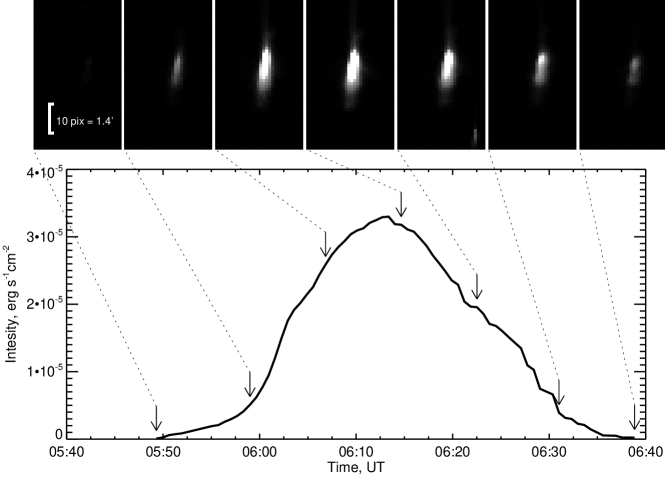
Figure 4.: Light curve of a HXP and corresponding date images. Times of images are marked on arrows.F:light˙curve

Figure. F:goes_mg_hxp shows a light curve of the same HXP, with a temporal dependence of Sun-integrated flux in $\lambda=8.42$ Å line and flux in the 1 – 8 Å GOES channel [Sylwester, Garcia, and Sylwester (1995)]. For clarity, flux in the 1 – 8 Å GOES channel is scaled (multiplied by 0.1). This figure shows that the intensity from separate HXP in $\lambda$ = 8.42 Å could amount to 5% of the total flux from the Sun in $\lambda$ = 8.42 Å.

Figure 5.: Temporal dependence of HXP intensity in the 8.42 Å line (solid line), Sun-integrated flux in 8.42 Å line (dashed line) and flux in 1 – 8 Å GOES channel (dotted line). For clarity, flux in 1 – 8 Å GOES channel is scaled (multiplied by 0.1)F:goes˙mg˙hxp

Urnov07 showed that there is strong linear correlation between the Mg xii spectroheliograph and GOES 1 – 8 Å fluxes. Peak HXP fluxes were estimated (see Figure F:GOES_class). Most of the HXPs are below A class.

Figure 6.: GOES class of HXPsF:GOES˙class

Examples of a light curve for different HXPs are shown in Figure F:4_light_curve. The lifetimes of these HXPs are approximately 10 minutes, 30 minutes, 50 minutes and 3 hours (we define lifetime as the time between the beginning and the ending of detection of the HXP in the 8.42 Å line). The intensity error is determined by the noise of the detector at low intensities and by photon statistics at high intensities.

Figure 7.: Intensity variation of HXPsF:4˙light˙curve

A histogram of HXPs’ lifetime is shown in Figure F:Time_hist. The most likely lifetime value is ten minutes, although HXPs with lifetime less than two minutes and greater than 60 minutes were observed 20 times, i.e. events with very short or very long lifetime are unlikely, but possible.

Figure 8.: HXP lifetimeF:Time˙hist

4 Determination of HXP Temperature

The HXP plasma temperature determination is based on measuring the spectral width of the Mg xii 8.42 Å line. In solar corona conditions the main contribution to line broadenings occurs due to the Doppler effect. Doppler broadening is caused by the thermal and turbulent motion of emitting ions. We neglect turbulence (because estimations show that its influence is small, see Appendix A:turb) and treat HXP plasma as isothermal. Then

$$\frac{\Delta\lambda}{\lambda}=\frac{1}{c}\sqrt{\frac{k_{B}T}{M}}\Rightarrow T=\frac{c^{2}M}{k_{B}}\left(\frac{\Delta\lambda}{\lambda}\right)^{2},\ilabel{E:temperature}$$ (2)

where $\Delta\lambda$ is the Doppler broadening, $\lambda$ = 8.42 Å, $c$ is the speed of light, $k_{B}$ is Boltzmann’s constant, $T$ is the plasma temperature, and $M$ is the mass of a magnesium ion.

Since only objects with small transverse sizes (relative to the direction of dispersion) were selected for analysis, we assume that their longitudinal size is also small. This means that a HXP’s intensity profile in the dispersion direction is a spectrum of Mg xii $\lambda=8.42$ Å line, undistorted by its spatial structure. Scanning of compact sources (in the dispersion direction) allows us in most cases to resolve both components of the Mg xii doublet. In order to obtain a doublet spectrum, the spectroheliograph signal was summed in the vicinity of a HXP in the direction perpendicular to the dispersion. This method is illustrated on Figure F:spectra_determination.

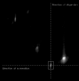
(a)                                (b)

Figure 9.: Magnesium doublet. a) Spectroheliograph image with HXP outlined (direction of dispersion is vertical, direction of summation is horizontal). b) Spectrum obtained after summation.F:spectra˙determination

The spectrum obtained was approximated by the sum of two Gauss profiles:

$$I(\lambda)=I_{1}\exp\left[-\frac{(\lambda-\lambda_{1})^{2}}{2\Delta\lambda^{2}}\right]+I_{2}\exp\left[-\frac{(\lambda-\lambda_{2})^{2}}{2\Delta\lambda^{2}}\right]+I_{0}$$ (3)

where $I(\lambda)$ is measured spectrum. $I_{1}$, $I_{2}$, $I_{0}$, $\lambda_{1}$, and $\Delta\lambda$ are unknown spectrum parameters, which are determined by fitting. The difference between $\lambda_{1}$ and $\lambda_{2}$ is fixed and equals 5.4 mÅ. It is worth mentioning that the temperature cannot always be determined: at low intensities, noise of the CCD corrupts the signal; also, sometimes the transverse size of the HXP could exceed one pixel, and therefore the temperature using the above method would not be accurate.

In Figure F:Temperature_curve, the variations of intensity and temperature of two HXPs are shown. The first event is relatively fast. It lasts ten minutes and the temperature reaches 20 MK. Maximum intensity and temperature occur approximately at the same time. The second HXP lasts 50 minutes, and the temperature reaches 30 MK. The maximum intensity is delayed by 20 minutes relative to maximum temperature. This effect is also seen for a number of other HXPs.

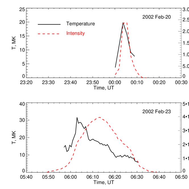
           (a)

           (b)

Figure 10.: Temporal variations of HXPs’ temperature and intensity. Solid line — temperature, dashed line — intensityF:Temperature˙curve

Let us mention that the temperature is always greater than 5 MK, and as the temperature reaches 5 MK, the intensity approaches zero. These two facts are in agreement with the contribution function of the Mg xii 8.42 Å line. The contribution function decreases rapidly when the temperature approaches 5 MK.

HXPs’ peak temperature (that is the maximum temperature reached during evolution of an individual HXP) lies in the range of 5 – 50 MK.

A histogram of the HXP’s peak temperature is shown in Figure F:Temperature_hist. The most likely value of the peak temperature is 12 MK.

Figure 11.: Weighted histogram of HXPs’ peak temperature. Each HXP is represented in the figure by a box of unit area, the width of which is $2\Delta T$.F:Temperature˙hist

The dependence of peak intensity on peak temperature is shown in Figure F:i_max_t_max. This figure shows that the two quantities are not correlated, i.e. more intense events are not necessarily hotter ones. Therefore, knowledge of peak intensity or peak temperature is not enough for the description of a HXP, but rather knowledge of other physical parameters is required.

Figure 12.: Dependence of HXPs’ peak intensity on peak temperature.F:i˙max˙t˙max

5 Absolute Intensity, Emission Measure, and Electron Density

The HXP’s emission measure is calculated from the absolute intensity and temperature. A histogram of HXP’s peak emission measure is shown in Figure F:em_hist. The HXP emission measure lies in the range of $10^{45}$–$10^{48}$ cm^-3.

Figure 13.: Histogram of HXPs’ peak emission measureF:em˙hist

If volume and emission of a source are known, its electron density could be determined. The size of an HXP cannot be measured, but we can make an estimation of its upper value (not greater than 5 Mm) and therefore arrive at an estimation of the lower limit of the electron density:

$$\ilabel{e:n_{e}st}n_{e}\geq\sqrt{\frac{EM}{h_{0}^{3}}}$$ (4)

This estimation gives us a value of $10^{10}$ cm^-3, which is higher than the typical value of electron density in the quiet corona ($10^{8}$ – $10^{9}$ cm^-3).

It is worth mentioning that an estimation of the sensitivity of the Mg xii spectroheliograph from the optical properties of the elements of which it consists (reflection coefficient of mirror on the working wavelength, detector sensitivity, etc.) is ten times higher than the value obtained by cross-calibration with GOES data. This means that obtained values of intensity and emission measure are accurate within a factor of ten. The uncertainty in the electron density would be three, which is acceptable for an estimation.

6 Dynamics of HXPs

For all 169 analyzed HXPs temporal variations of intensity, temperature, emission measure, and electron density were obtained. HXPs could be divided into two groups by the behavior of these parameters: those with gradually decreasing temperatures and those with rapidly decreasing temperatures.

Let us consider the first group (see Figure F:T_I_n_EM). HXPs of this group have low intensity and emission measure at the beginning of their lifetime; their temperature lies in the range of 10 – 15 MK. During a period of approximately five minutes, their intensity and emission measure increase slowly, and the temperature is roughly constant. Then the temperature reaches extremely high values (30 – 50 MK) over a period of 2 – 5 minutes, while its emission measure reaches a maximum, and intensity increases with the same rate. After reaching its maximum temperature, the HXP cools down to 5 MK between 5 – 30 minutes, while the emission measure slowly decreases. The intensity reaches its maximum after maximum temperature. As the temperature approaches 5 MK, the intensity approaches zero. Since the cadence of the spectroheliograph is limited, for some events the phase of temperature increase is not seen. That is why some events are seen beginning from high temperatures (30 – 50 MK). This behavior of HXP parameters could be explained by the following scenario: at some moment in time, a process of energy release in the volume of HXP begins. As a result, the HXP temperature increases and reaches its maximum. Then the power of the energy release decreases and the HXP starts to slowly cool down. HXPs of this group are 39% of the whole of observed HXPs.

        (a)                                 (b)

        (c)                                 (d)

Figure 14.: Variation of intensity (a), emission measure (b), temperature (c), and electron density (d) of an HXP of the first group (23 February 2002).F:T˙I˙n˙EM

                             (a)                                 (b)

                             (c)                                 (d)

Figure 15.: Intensity (a), emission measure (b), temperature (c), and electron density (d) of an HXP of the second group (28 February 2002).F:T˙I˙n˙EM˙2nd

Let us describe the behavior of the second group (see Figure F:T_I_n_EM_2nd). HXPs of this group have an abrupt jump in temperature to high values (30 – 50 MK) over a short period of time (2 – 5 minutes) with slowly changing intensity. The HXP, after reaching its maximum temperature, cools down rapidly to 10 – 20 MK in 2 – 5 minutes. After this, the temperature stops changing and remains constant during the latter part of its lifetime (10 – 30 min). Intensity and emission measure reach their maxima when the temperature remains constant. After reaching its maximum intensity and maximum emission measure, intensity and emission measure simultaneously decrease slowly to zero. Since the cadence of the spectroheliograph is limited, the temperature increase phase is not seen. That is why some events are seen beginning from stationary temperatures (10 – 20 MK). The HXPs of the first group disappear because their temperatures leave the range, which can be seen using a spectroheliograph. The HXPs of the second group disappear because their emission measures approach zero. A decrease in the emission measure could take place because of the expanding (increasing volume) of the HXP or because of a decrease of electron density (or both). HXPs of the second group represent 40% of the whole observed HXPs.

In addition to these two groups, there were very short events with lifetimes of two – three minutes. These events were seen during only two – four frames, and therefore very little can be said about their variation. Fast HXPs are 20% of the observed HXPs.

7 Spatial Distribution of HXP

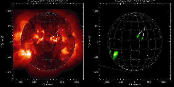
                              (a)                                (b)

Figure 16.: Yohkoh/SXT (a) and Mg xii spectroheliograph (b). HXPs, which are loop footpoints, are marked with arrows.F:loop˙footpoint

In order to investigate possible connection between HXPs and active regions, the Mg xii spectroheliograph compared with Yohkoh/SXT images. Yohkoh/SXT has a wide temperature range ($T>$ 2 MK), which includes hot plasma ($T>$ 5 MK, which is seen in the Mg xii spectroheliograph) and cool components ($T$ = 2 – 5 MK, in which active regions are seen). Between August and December 2001 both satellites were operating, and a comparison could be carried out at this period of time.

Examples of such frames are shown in Figure F:compact_structure and Figure F:loop_footpoint. In Figure F:compact_structure images of Yohkoh/SXT and spectroheliograph taken within one hour are shown. HXPs, which are compact structures, are marked with arrows 1 – 3. In Figure F:loop_footpoint images of Yohkoh/SXT and spectroheliograph taken at close points in time are shown. HXPs, which are loop footpoints, are marked with arrows. So HXPs could be a compact structure or be a part of an active region (footpoints of its loops).

In Figure F:Space_distribution the spatial distribution of HXPs over the Sun’s surface is shown. In order to build this map, coordinates of 169 HXPs observed between 2002 20 and 28 February were used. Figure F:Space_distribution shows that HXPs are concentrated in the active-region bands. Microflares are also concentrated in the active region bands [Christe et al. (2008)]. X-ray bright points (XBP) are uniformly spread over the solar surface [Golub et al. (1974)]. Thus, HXPs have a similar spatial distribution with microflares but are different than XBPs.

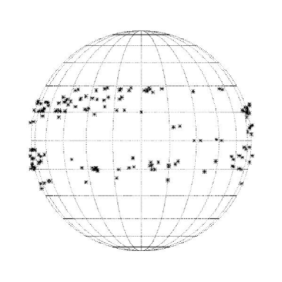
Figure 17.: Spatial distribution of HXPsF:Space˙distribution

8 Cooling Time and Energy of HXP

Comparison of heating and cooling times of HXPs with conductive and radiative cooling rate will allow us to study the heating mechanism. A typical value of a HXP heating time is five minutes; the cooling time lies in the range of 2 – 30 minutes. Let us compare these values with radiative and conductive cooling times.

The conductive cooling time $\tau_{\mathrm{cond}}$ is [Culhane et al. (1994)]

$$\tau_{\mathrm{cond}}=\frac{21n_{e}k_{B}h^{2}}{5\kappa T^{5/2}}=\frac{21k_{B}\sqrt{EM\cdot h}}{5\kappa T^{5/2}}\leq\frac{21k_{B}\sqrt{EM\cdot h_{0}}}{5\kappa T^{5/2}}=15\ \textmd{s}$$ (5)

(where $\kappa=9.2\times 10^{-7}\ \textmd{erg}\ \textmd{s}^{-1}\textmd{cm}^{-1}\textmd{K}^{-7/2}$ is the Spitzer conductivity, $EM\approx 10^{47}\ \textmd{cm}^{-3}$ is the HXP emission measure, $T\approx 10^{7}\ \textmd{K}$ is the HXP temperature, $h$ is the source size, $h_{0}$ is the effective pixel size).

Let us estimate the influence of radiative losses. The radiative loss rate is

$$P_{\mathrm{rad}}=EM\ \Lambda(T),$$ (6)

where $\Lambda(T)\approx 10^{-22}\ \textmd{erg}\ \textmd{cm}^{3}\ \textmd{s}^{-1}$ is the radiative loss function [Klimchuk, Patsourakos, and Cargill (2008)].

The conductive loss rate is

$$P_{\mathrm{cond}}=\kappa S\frac{\partial T}{\partial x}\sim\kappa T^{\frac{5}{2}}h^{2}\frac{T}{h}=\kappa T^{\frac{7}{2}}h$$ (7)

Let us compare these two quantities:

$$\frac{P_{\mathrm{cond}}}{P_{\mathrm{rad}}}\sim\frac{\kappa T^{\frac{7}{2}}h}{EM\cdot\Lambda(T)}\sim 10^{2}$$ (8)

so radiative losses can be neglected.

The conductive cooling time is significantly lower than the HXP lifetime, heating time, and cooling time. This means that energy release in the HXP volume occurs throughout its lifetime.

HXP thermal energy $\varepsilon_{\mathrm{th}}$ can be estimated as

$$\varepsilon_{\mathrm{th}}\sim nVk_{B}T=k_{B}T\sqrt{EM\ V}\leq k_{B}T\sqrt{EM\ h_{0}^{3}}=10^{28}\ \textmd{erg}$$ (9)

$\varepsilon_{\mathrm{th}}$ is four orders lower than thermal energy of the most powerful flares ($4\times 10^{32}$ erg: hud83). This means that HXPs could be classified by thermal energy scale as a micro-scale events.

Since HXP lifetime is significantly greater than $\tau_{\mathrm{cond}}$, the power, which is heating the HXP, must be approximately equal to conductive losses:

$$P\approx\frac{\varepsilon_{\mathrm{th}}}{\tau_{\mathrm{cond}}}\approx 10^{27}\ \textmd{erg\ s${}^{-1}$}$$ (10)

The total energy, which is released inside HXP, equals

$$\varepsilon_{\mathrm{total}}\approx P\ \tau_{\mathrm{total}}\approx 10^{30}\ \textmd{erg},$$ (11)

where $\tau_{\mathrm{total}}$ is the HXP lifetime.

9 HXPs and Other Microactivity Phenomena

Let us compare measured HXP physical parameters with parameters of other flare-like microevents: microflares [Christe et al. (2008), Hannah et al. (2008)], XBPs [Golub, Krieger, and Vaiana (1976), Golub and Pasachoff (1997)] and nanoflares [Parker (1988), Aschwanden et al. (2000)]. The parameters of these phenomena are listed in Table L:events.

Table 1.: Comparison of parameters of HXPs and other microactivity phenomenaL:events

	HXP	XBP	microflares	nanoflares
Lifetime	5 – 100 min	8 – 40 h	1 – 10 min	1 – 3 hr
$T$[MK]	5 – 50	1 – 2	10 – 15	1 – 2
$EM$[cm-3]	$10^{45}$ – $10^{48}$	$\approx 10^{47}$	$10^{45}$ – $10^{48}$	$\approx 10^{44}$
$n_{e}$[cm-3]	$\geq 10^{10}$	$\approx 5\cdot 10^{9}$	$10^{9}$ – $10^{11}$	$10^{8}$ – $10^{9}$
Size[Mm]	$\leq 5$	$\approx 25$	5 – 25	2 – 20

Table L:events shows that HXPs differ significantly from XBPs and nanoflares in their lifetimes, temperatures, and sizes. HXPs have higher emission measures and electron densities than nanoflares. HXPs differ from XBPs in their spatial distribution over the solar surface.

HXPs and microflares have the same range of values of emission measure, electron density, and thermal energy. Also they have the same spatial distribution over the solar surface (they are concentrated in the active-region latitudes). Nonetheless, HXPs have longer lifetimes, higher temperatures, and smaller sizes than microflares.

Taking into account these arguments, we conclude that HXPs, nanoflares, and XBPs are different phenomena. The differences between HXPs and microflares are less clear, and we cannot rule out the possibility that they belong to a similar class of phenomena.

Appendix A Influence of Turbulence

A:turb

Turbulence contributes to Mg xii ion line broadening:

$$\left(\frac{\Delta\lambda}{\lambda}\right)^{2}=\frac{k_{B}T}{M}+u^{2}_{\mathrm{turb}},\ilabel{E:Doppler_{t}urb}$$ (12)

where $M$ is the mass of magnesium ion, $u_{\mathrm{turb}}$ is the turbulence velocity. Equation (E:Doppler_turb) shows that turbulence increases the value of the effective temperature, obtained by our method, by the amount:

$$\Delta T_{\mathrm{turb}}=\frac{Mu_{\mathrm{turb}}^{2}}{k_{\mathrm{B}}}$$ (13)

The uncertainty in the temperature in our work is $\Delta T_{\mathrm{err}}\approx$ 1–2 MK. If $u_{\mathrm{turb}}=$ 30 km s^-1, then $\Delta T_{\mathrm{turb}}$ will be equal to $\Delta T_{\mathrm{err}}$. That means that only high values of turbulence will affect the value of the temperature obtained. If $u_{\mathrm{turb}}$ is less than or equal to 30 km s^-1 then the $\Delta T_{\mathrm{turb}}$ will be less than the error of our method. That is why we neglect turbulence in our work.

Figure F:Temperature_hist shows a histogram of HXP peak temperatures. It has a maximum around 12 MK and a high-temperature flat tail, which starts at 20 MK and ends at 50 MK. This tail could be caused by nonthermal line broadening due to turbulence. If we suppose that the “true” temperatures of HXPs of this tail are around 10 MK, then the $\Delta T_{\mathrm{turb}}$ will be 30 MK, which would arise from $u_{\mathrm{turb}}\approx$ 180 km s^-1. This is a very high value, but nonetheless possible. Such values are encountered in large solar flares [Kay et al. (2006)].

High observed temperatures could indeed be caused by nonthermal broadening due to turbulence. But such an explanation requires an assumption of high turbulence velocities.

Acknowledgements

The authors acknowledge the help of A.M. Urnov, N.K. Suhodrev, and J. Sylwester with preparing of this article for publication. The work was supported by the Russian Foundation of Basic Research (grant 11-02-01079a), by a grant of the President of Russian Federation (MK-3875.2011.2), and the SOTERIA project of Programme FP7/2007-2013 (grant 218816).

References

- Aschwanden et al. (2000) Aschwanden, M.J., Tarbell, T.D., Nightingale, R.W., Schrijver, C.J., Title, A., Kankelborg, C.C., Martens, P., Warren, H.P.: 2000, Time Variability of the “Quiet” Sun Observed with TRACE. II. Physical Parameters, Temperature Evolution, and Energetics of Extreme-Ultraviolet Nanoflares. ApJ 535, 1047 – 1065. doi:10.1086/308867.
- Benz and Grigis (2002) Benz, A.O., Grigis, P.C.: 2002, Microflares and hot component in solar active regions. Sol. Phys. 210, 431 – 444. doi:10.1023/A:1022496515506.
- Christe et al. (2008) Christe, S., Hannah, I.G., Krucker, S., McTiernan, J., Lin, R.P.: 2008, RHESSI Microflare Statistics. I. Flare-Finding and Frequency Distributions. ApJ 677, 1385 – 1394. doi:10.1086/529011.
- Culhane et al. (1994) Culhane, J.L., Phillips, A.T., Inda-Koide, M., Kosugi, T., Fludra, A., Kurokawa, H., Makishima, K., Pike, C.D., Sakao, T., Sakurai, T.: 1994, YOHKOH observations of the creation of high-temperature plasma in the flare of 16 December 1991. Sol. Phys. 153, 307 – 336. doi:10.1007/BF00712508.
- Golub and Pasachoff (1997) Golub, L., Pasachoff, J.M.: 1997, The Solar Corona, Cambridge University Press, Cambridge, UK.
- Golub, Krieger, and Vaiana (1976) Golub, L., Krieger, A.S., Vaiana, G.S.: 1976, Observation of spatial and temporal variations in X-ray bright point emergence patterns. Sol. Phys. 50, 311 – 327. doi:10.1007/BF00155294.
- Golub et al. (1974) Golub, L., Krieger, A.S., Silk, J.K., Timothy, A.F., Vaiana, G.S.: 1974, Solar X-Ray Bright Points. ApJ 189, L93. doi:10.1086/181472.
- Golub et al. (2007) Golub, L., Deluca, E., Austin, G., Bookbinder, J., Caldwell, D., Cheimets, P., Cirtain, J., Cosmo, M., Reid, P., Sette, A., Weber, M., Sakao, T., Kano, R., Shibasaki, K., Hara, H., Tsuneta, S., Kumagai, K., Tamura, T., Shimojo, M., McCracken, J., Carpenter, J., Haight, H., Siler, R., Wright, E., Tucker, J., Rutledge, H., Barbera, M., Peres, G., Varisco, S.: 2007, The X-Ray Telescope (XRT) for the Hinode Mission. Sol. Phys. 243, 63 – 86. doi:10.1007/s11207-007-0182-1.
- Hannah et al. (2008) Hannah, I.G., Christe, S., Krucker, S., Hurford, G.J., Hudson, H.S., Lin, R.P.: 2008, RHESSI Microflare Statistics. II. X-Ray Imaging, Spectroscopy, and Energy Distributions. ApJ 677, 704 – 718. doi:10.1086/529012.
- Hudson and Willson (1983) Hudson, H.S., Willson, R.C.: 1983, Upper limits on the total radiant energy of solar flares. Sol. Phys. 86, 123 – 130. doi:10.1007/BF00157181.
- Kay et al. (2006) Kay, H.R.M., Matthews, S.A., Harra, L.K., Culhane, J.L.: 2006, Non-thermal broadening of coronal emission lines in the onset phase of solar flares and CMEs. A&A 447, 719 – 725. doi:10.1051/0004-6361:20053240.
- Klimchuk, Patsourakos, and Cargill (2008) Klimchuk, J.A., Patsourakos, S., Cargill, P.J.: 2008, Highly Efficient Modeling of Dynamic Coronal Loops. ApJ 682, 1351 – 1362. doi:10.1086/589426.
- Kosugi et al. (2007) Kosugi, T., Matsuzaki, K., Sakao, T., Shimizu, T., Sone, Y., Tachikawa, S., Hashimoto, T., Minesugi, K., Ohnishi, A., Yamada, T., Tsuneta, S., Hara, H., Ichimoto, K., Suematsu, Y., Shimojo, M., Watanabe, T., Shimada, S., Davis, J.M., Hill, L.D., Owens, J.K., Title, A.M., Culhane, J.L., Harra, L.K., Doschek, G.A., Golub, L.: 2007, The Hinode (Solar-B) Mission: An Overview. Sol. Phys. 243, 3 – 17. doi:10.1007/s11207-007-9014-6.
- Lin et al. (1984) Lin, R.P., Schwartz, R.A., Kane, S.R., Pelling, R.M., Hurley, K.C.: 1984, Solar hard X-ray microflares. ApJ 283, 421 – 425. doi:10.1086/162321.
- Lin et al. (2002) Lin, R.P., Dennis, B.R., Hurford, G.J., Smith, D.M., Zehnder, A., Harvey, P.R., Curtis, D.W., Pankow, D., Turin, P., Bester, M., Csillaghy, A., Lewis, M., Madden, N., van Beek, H.F., Appleby, M., Raudorf, T., McTiernan, J., Ramaty, R., Schmahl, E., Schwartz, R., Krucker, S., Abiad, R., Quinn, T., Berg, P., Hashii, M., Sterling, R., Jackson, R., Pratt, R., Campbell, R.D., Malone, D., Landis, D., Barrington-Leigh, C.P., Slassi-Sennou, S., Cork, C., Clark, D., Amato, D., Orwig, L., Boyle, R., Banks, I.S., Shirey, K., Tolbert, A.K., Zarro, D., Snow, F., Thomsen, K., Henneck, R., McHedlishvili, A., Ming, P., Fivian, M., Jordan, J., Wanner, R., Crubb, J., Preble, J., Matranga, M., Benz, A., Hudson, H., Canfield, R.C., Holman, G.D., Crannell, C., Kosugi, T., Emslie, A.G., Vilmer, N., Brown, J.C., Johns-Krull, C., Aschwanden, M., Metcalf, T., Conway, A.: 2002, The Reuven Ramaty High-Energy Solar Spectroscopic Imager (RHESSI). Sol. Phys. 210, 3 – 32. doi:10.1023/A:1022428818870.
- Ogawara et al. (1991) Ogawara, Y., Takano, T., Kato, T., Kosugi, T., Tsuneta, S., Watanabe, T., Kondo, I., Uchida, Y.: 1991, The Solar-A Mission - an Overview. Sol. Phys. 136, 1 – 16. doi:10.1007/BF00151692.
- Parker (1988) Parker, E.N.: 1988, Nanoflares and the solar X-ray corona. ApJ 330, 474 – 479. doi:10.1086/166485.
- Shimizu (1995) Shimizu, T.: 1995, Energetics and Occurrence Rate of Active-Region Transient Brightenings and Implications for the Heating of the Active-Region Corona. PASJ 47, 251 – 263.
- Sylwester, Garcia, and Sylwester (1995) Sylwester, J., Garcia, H.A., Sylwester, B.: 1995, Quantitative interpretation of GOES soft X-ray measurements. I. The isothermal approximation: application of various atomic data. A&A 293, 577 – 585.
- Tsuneta et al. (1991) Tsuneta, S., Acton, L., Bruner, M., Lemen, J., Brown, W., Caravalho, R., Catura, R., Freeland, S., Jurcevich, B., Owens, J.: 1991, The soft X-ray telescope for the SOLAR-A mission. Sol. Phys. 136, 37 – 67. doi:10.1007/BF00151694.
- Urnov et al. (2007) Urnov, A.M., Shestov, S.V., Bogachev, S.A., Goryaev, F.F., Zhitnik, I.A., Kuzin, S.V.: 2007, On the spatial and temporal characteristics and formation mechanisms of soft X-ray emission in the solar corona. Astron. Lett. 33, 396 – 410. doi:10.1134/S1063773707060059.
- Zhitnik et al. (2003a) Zhitnik, I.A., Bugaenko, O.I., Ignat’ev, A.P., Krutov, V.V., Kuzin, S.V., Mitrofanov, A.V., Oparin, S.N., Pertsov, A.A., Slemzin, V.A., Stepanov, A.I., Urnov, A.M.: 2003a, Dynamic 10 MK plasma structures observed in monochromatic full-Sun images by the SPIRIT spectroheliograph on the CORONAS-F mission. MNRAS 338, 67 – 71. doi:10.1046/j.1365-8711.2003.06014.x.
- Zhitnik et al. (2003b) Zhitnik, I., Kuzin, S., Afanas’ev, A., Bugaenko, O., Ignat’ev, A., Krutov, V., Mitrofanov, A., Oparin, S., Pertsov, A., Slemzin, V., Sukhodrev, N., Umov, A.: 2003b, XUV observations of solar corona in the spirit experiment on board the coronas-F satellite. Adv. Spa. Res. 32, 473 – 477. doi:10.1016/S0273-1177(03)00351-X.