Abundance gradients in low surface brightness spirals: clues on the origin of common gradients in galactic discs

Abstract

We acquired spectra of 141 H ii regions in ten late-type low surface brightness galaxies (LSBGs). The analysis of the chemical abundances obtained from the nebular emission lines shows that metallicity gradients are a common feature of LSBGs, contrary to previous claims concerning the absence of such gradients in this class of galaxies. The average slope, when expressed in units of the isophotal radius, is found to be significantly shallower in comparison to galaxies of high surface brightness. This result can be attributed to the reduced surface brightness range measured across their discs, when combined with a universal surface mass density–metallicity relation. With a similar argument we explain the common abundance gradient observed in high surface brightness galaxy (HSBG) discs and its approximate dispersion. This conclusion is reinforced by our result that LSBGs share the same common abundance gradient with HSBGs, when the slope is expressed in terms of the exponential disc scale length.

1 Introduction

During the past few decades the investigation of the radial chemical abundance gradients of spiral galaxies has provided critical constraints for our understanding of their evolutionary histories. The overall picture that emerges from a large body of observational work on the oxygen abundances (O/H) of extragalactic H ii regions, the standard tracers of metals in star-forming galaxies (see Pilyugin, Grebel & Kniazev 2014a for a recent compilation), is consistent with an inside-out growth of galactic discs, in which the abundance gradients reflect radial variations of star formation rates and gas infall timescales (Prantzos & Boissier 2000; Fu et al. 2013).

Recent observational work on the chemical composition of spiral galaxies has addressed a number of topics, in particular the use of abundance diagnostics that are complementary to H ii regions, such as blue supergiant stars (Kudritzki et al. 2008, 2012; Bresolin et al. 2009b) and planetary nebulae (Bresolin et al. 2010; Stasińska et al. 2013), azimuthal variations (Li, Bresolin & Kennicutt 2013; Sánchez et al. 2015), the flattening of the gradients at large galactocentric distances (Bresolin et al. 2009a; Bresolin, Kennicutt & Ryan-Weber 2012; Marino et al. 2012) and in interacting systems (Kewley et al. 2010; Rich et al. 2012), and the spatial distributions of metals in high-redshift galaxies (Yuan et al. 2011; Queyrel et al. 2012; Jones et al. 2013). Moreover, integral field spectroscopy is currently providing abundance gradients for large samples of nearby galaxies (Rosales-Ortega et al. 2010; Sánchez et al. 2014), yielding high statistical significance to correlations with global galactic properties and scaling relations.

Despite this progress, the abundance gradient properties of low surface brightness galaxies (LSBGs), a significant component of the overall galaxy population (e.g. Impey & Bothun 1997), remain virtually unknown, largely as a result of observational challenges. Chemical abundances of late-type LSBGs have insofar been obtained either from emission line spectroscopy of the central portions of compact systems (Burkholder, Impey & Sprayberry 2001; Bergmann, Jørgensen & Hill 2003; Liang et al. 2010) or from individual H ii regions, but with insufficient numbers to derive reliable radial trends (McGaugh 1994; Rönnback & Bergvall 1995; Kuzio de Naray, McGaugh & de Blok 2004). To date the only attempt to constrain the oxygen abundance gradient in LSBGs has been reported by de Blok & van der Hulst (1998), who, examining nebular abundances in three LSBGs, concluded that their radial distributions are flat.

The typical oxygen abundances of LSBGs span a wide range, from 12 + log(O/H) $<$ 8.4 (McGaugh 1994; Rönnback & Bergvall 1995) up to super-solar values (Bergmann et al. 2003), but on average peaking below the characteristic abundances measured in high surface brightness galaxies (Liang et al. 2010). For example, Burkholder et al. (2001) found a mean value 12 + log(O/H) = 8.22 for 17 LSBGs, compared to 12 + log(O/H) = 8.47 for 49 high surface brightness galaxies.

The relatively low metallicities, together with small star formation rates and blue optical and near-infrared colors, corroborate the notion that LSBGs are slowly-evolving systems (de Blok, van der Hulst & Bothun 1995; van den Hoek et al. 2000), with small-amplitude bursts on top of star formation rates that are nearly constant when integrated over Gyr timescales (Gerritsen & de Blok 1999; Bell et al. 2000; Boissier et al. 2008; Schombert & McGaugh 2014). The reported lack of chemical abundance gradients has been regarded as supporting evidence for star formation histories characterized by sporadic episodes, and possibly linked to a mode of galactic evolution that does not proceed from the inside out (de Blok & van der Hulst 1998; Vorobyov et al. 2009).

The present work stems from one main motivation. The study by de Blok & van der Hulst (1998), which remains to date the only investigation of the radial abundance trends in LSBGs, reached its conclusion about the lack of detectable gradients on the basis of only three galaxies, with a relatively small number ($4\leq n\leq 7$) of H ii region spectra obtained per galaxy. Perhaps more importantly, all three systems have an irregular morphological type. Abundance gradients in such galaxies are generally found to be very weak or absent (e.g. van Zee & Haynes 2006; Croxall et al. 2009), although Pilyugin, Grebel & Zinchenko (2015) recently measured significant gradients in a number of irregular galaxies.

Therefore, in order to verify claims, based on the chemical abundance properties, that LSBGs evolve differently (aside from the slower evolution) compared to galaxies of high surface brightness, it is essential to characterize the abundance gradients of LSBGs displaying a spiral morphology. Currently, multi-object techniques on 8m-class telescopes make the spectroscopy of relatively large samples of H ii regions, necessary to obtain reliable estimates of the abundance gradients, feasible even with moderate amounts of observing time.

In this paper we present new oxygen abundances of H ii regions in 10 late-type LSBGs, with the main goal of deriving their radial distributions. Our observational material is presented in Sect. 2, and we derive nebular chemical abundances using different diagnostics in Sect. 3. We discuss the abundance gradients in Sect. 4 and summarize our results in Sect. 5.

2 Observations and data reduction

2.1 Observations

Table 1: Galaxy sample.

ID	R.A. (J2000)	Dec. (J2000)	Type	D	$M_{B}$	PA	i	$r_{25}$	$r_{d}$	$\mu_{B}(0)$	Ref.
	h   m   s	$\circ$   $\prime$   $\prime\prime$		Mpc		deg		arcsec (kpc)		mag arcsec-2
(1)	(2)	(3)	(4)	(5)	(6)	(7)	(8)	(9)	(10)	(11)	(12)
ESO 059-009	07 36 13.08	$-$70 42 40.2	Sd	16.7	$-$17.7	169	27	49 (3.9)	27 (2.1)	23.1	a
ESO 187-051	21 07 32.78	$-$54 57 09.1	Sm	17.8	$-$16.8	11	52	40 (3.5)	26 (2.2)	23.1	1,b
ESO 249-036	03 59 15.72	$-$45 52 20.7	Sm	9.7	$-$14.9	156	15	35 (1.7)	37 (1.7)	24.0	1,b
ESO 440-049	12 05 34.07	$-$31 25 25.4	Sc	31.2	$-$19.0	62	42	45 (6.9)	18 (2.7)	23.1	2,a
ESO 446-053	14 21 17.08	$-$29 15 47.6	Sdm	17.1	$-$17.9	165	67	53 (4.4)	28 (2.3)	22.9⋆	3,c
ESO 504-025	11 53 50.15	$-$27 20 59.2	Sd	24.1	$-$17.5	20	40	21 (2.5)	20 (2.3)	23.9⋆	3,c
ESO 510-026	13 57 35.77	$-$25 47 27.4	Scd	33.4	$-$17.8	130	37	31 (5.1)	13 (2.1)	22.4⋆	3,c
UGC 1230	01 45 32.50	$+$25 31 14.8	Sc	57.0	$-$17.6	112	22	24 (6.5)	16 (4.4)	23.3	4,5,7,d
UGC 6151	11 05 56.27	$+$19 49 34.9	Sc-Sm	21.3	$-$16.9	175	18	39 (4.1)	24 (2.5)	23.2	6,5,7,d
UGC 9024	14 06 40.55	$+$22 04 12.4	Sc-Sm	36.5	$-$16.4	148	15	18 (3.3)	35 (6.2)	24.5	5,7,d

$(1)$ PA, i from Auld et al. (2006). $(2)$ $\mu_{B}(0)$ from Beijersbergen et al. (1999), using $\mu_{R}(0)$ and the average $\mu_{B}(0)-\mu_{R}(0)$ in their Table 2. $(3)$ PA, i, Type from Matthews & Gallagher (1997). $(4)$ PA, i from van der Hulst et al. (1993). $(5)$ Type from McGaugh et al. (1995). $(6)$ PA, i from Patterson & Thuan (1996). $(7)$ $r_{d}$ from McGaugh & Bothun (1994).

Sources for the B-band exponential disc scalelength $r_{d}$: (a) Beijersbergen et al. (1999) (R-band for ESO 440-049); (b) Bell et al. (2000); (c) Lauberts & Valentijn (1989); (d) McGaugh & Bothun (1994).

^⋆ Not a published value, but derived from the expression $\mu_{o}(B)=25-r_{25}/r_{d}$.

LSBGs are often characterized by sparse distributions of faint H ii regions, which make it difficult to derive reliable chemical abundance gradients. For our study we selected galaxies that were shown by previous work to contain a sufficient number of H ii regions to alleviate such a difficulty. Our targets were extracted from a variety of sources providing imaging and surface photometry information: Beijersbergen, de Blok & van der Hulst (1999), Auld et al. (2006), de Blok et al. (1995), McGaugh & Bothun (1994) and McGaugh, Schombert & Bothun (1995). The galaxies selected have $B$-band central disc surface brightness $\mu_{B}(0)>23$ mag arcsec^-2, a value that is commonly adopted to define LSBGs (e.g. Impey & Bothun 1997), being more than one magnitude fainter than the canonical Freeman (1970) value $\mu_{B}(0)=21.65\pm 0.3$ mag arcsec^-2 (this is somewhat arbitrary, and some authors use, for instance, $\mu_{B}(0)=22$ mag arcsec^-2 as the dividing line between low and high surface brightness galaxies, HSBGs; e.g. Burkholder et al. 2001; Boissier et al. 2003; Liang et al. 2010). We also included three targets from the list of extreme late-type spiral galaxies by Matthews & Gallagher (1997). Although the value of their central disc surface brightness is not reported in their work, these systems have structural and global surface brightness characteristics that are comparable to those of the remaining targets in our sample. Their $\mu_{B}(0)$ values were estimated from the expression $\mu_{B}(0)=25-r_{25}/r_{d}$, using the values for $r_{25}$ and $r_{d}$ from Lauberts & Valentijn (1989), and range between 22.4 and 23.9 mag arcsec^-2.

Our final sample of 10 LSBGs comprises systems both with and without bulge, and is presented in Table 1, where most of the information has been extracted from the HyperLeda database (Makarov et al. 2014). The exceptions are reported in the last column of the table. The celestial coordinates of the galactic centers were measured from our astrometrically calibrated images (see below). We follow the nomenclature from the ESO/Uppsala survey (Lauberts 1982) and the Uppsala General Catalogue of galaxies (UGC, Nilson 1973). We re-classified ESO 249-036 (Horologium dwarf, part of a pair with ESO 249-035) as an Sm type (instead of Im; e.g. Lauberts 1982), based on the patchy, arm-like structure shown in the images by Auld et al. (2006, classified this galaxy as an Sdm). For all the remaining galaxies we retain the late-type spiral (Sc to Sm) classification given in the sources specified in Table 1.

We obtained spectra of individual H ii regions in the target galaxies with two different instruments and multi-slit setups: the Very Large Telescope (VLT) equipped with the FOcal Reducer and low dispersion Spectrograph (FORS) and the Gemini North telescope with the Multi-Object Spectrograph (GMOS). The FORS data (collected for the seven ESO galaxies) were obtained with the 300V grism using 0$\aas@@fstack{\prime\prime}$9 slits, while the GMOS data (for the three UGC galaxies) were obtained with the B600 grating using 1$\aas@@fstack{\prime\prime}$4 slits.

The slit masks were designed based on narrow-band H$\alpha$ imaging (on- and off-band) secured in advance of the spectroscopic runs. For six of the galaxies we used two separate masks, in order to increase the number of target H ii regions. The number of H ii regions observed per galaxy ranges between 7 and 21. The total exposure times, reported in Table 2, range between 3600 s and 6000 s, and were subdivided into a number of sub-exposures varying from three to six. The spectral coverage extends from approximately 3650 Å to 7000 Å, with a FWHM spectral resolution of 8 Å (FORS) and 4.8 Å (GMOS). Thus all the main nebular emission-line diagnostics, from [O ii]$\,\lambda$3727 to [S ii]$\,\lambda\lambda$6717,31, are accessible, and [N ii]$\,\lambda$6583 is easily deblended from H$\alpha$.

2.2 Data reduction

Bias subtraction, flat-field correction and wavelength calibration were accomplished with the European Southern Observatory’s EsoRex pipeline for the FORS data, and iraf routines in the gemini/gmos package for the GMOS data. Flux calibration using standard star spectrophotometry, coaddition of sub-exposures and extraction to one-dimensional spectra yielded the final data products to be analyzed. Emission line fluxes were measured non-interactively with the fitprofs tool in iraf.

The line fluxes were corrected for interstellar reddening by comparing the H$\alpha$/H$\beta$ and H$\gamma$/H$\beta$  ratios to the corresponding case B values at $10^{4}$ K, requiring that the two line ratios yield a consistent extinction coefficient c(H$\beta$), by adjusting the equivalent width of the underlying absorption component. The reddening-corrected line fluxes for the [O ii]$\,\lambda$3727, [O iii]$\,\lambda$5007, [N ii]$\,\lambda$6583 and [S ii]$\,\lambda\lambda$6717,6731 emission lines, that are used as metallicity diagnostics, are reported, in units of $f$(H$\beta$) = 100, in Table 3 (the printed version reports the information for ESO 059-009 only, while the complete table is available in the online version of the journal). We include the detections of the [O iii]$\,\lambda$4363 line, which can be used, in combination with [O iii]$\,\lambda$5007, to obtain direct estimates of the gas electron temperature. The errors quoted include the statistical and flux calibration errors, and the uncertainty in the reddening correction. We confirmed that the relative strengths of the emission lines are consistent with those expected for photoionized nebulae, as judged from the appropriate diagnostic diagrams (e.g. Baldwin, Phillips & Terlevich 1981).

Table 2: Log of the observations.

Galaxy	Date	Exp. time (s)
ESO 059-009	2012 Apr 17,18	6000 ($\times$2 fields)
ESO 187-051	2011 June 25,26	5094
ESO 249-036	2011 Mar 04,05	5094
ESO 440-049	2012 Apr 17	6000 ($\times$2 fields)
ESO 446-053	2012 Apr 17,18	3600 ($\times$2 fields)
ESO 504-025	2012 Apr 18	6000 ($\times$2 fields)
ESO 510-026	2012 Apr 17	6000
UGC 1230	2010 Sept 11,12	3600 ($\times$2 fields)
UGC 6151	2011 May 04	4500
	2012 Mar 20	4500
UGC 9024	2011 June 20,30	4500
	2012 Feb 26, Apr 15	4500

Table 3: Reddening-corrected fluxes: ESO 059-009

ID	R.A.	Dec.	$r/r_{25}$	[O ii]	[O iii]	[O iii]	[N ii]	[S ii]	c(H$\beta$)	F(H$\beta$)
	(J2000.0)	(J2000.0)		3727	4363	5007	6583	6731+6717		(erg s-1 cm-2)
(1)	(2)	(3)	(4)	(5)	(6)	(7)	(8)	(9)	(10)	(11)
1	07 36 12.4	$-70$ 42 03.50	0.76	179 $\pm$ 9	…	33 $\pm$ 2	71 $\pm$ 4	76 $\pm$ 3	0.21	1.5 $\times\ 10^{-16}$
2	07 36 08.1	$-70$ 42 09.10	0.84	190 $\pm$ 10	…	37 $\pm$ 2	67 $\pm$ 4	70 $\pm$ 3	0.26	1.1 $\times\ 10^{-15}$
3	07 36 10.6	$-70$ 42 10.62	0.66	172 $\pm$ 9	…	45 $\pm$ 2	69 $\pm$ 4	51 $\pm$ 2	0.46	1.5 $\times\ 10^{-16}$
4	07 36 13.1	$-70$ 42 24.78	0.32	116 $\pm$ 7	…	0 $\pm$ 1	70 $\pm$ 4	66 $\pm$ 3	0.43	7.9 $\times\ 10^{-17}$
5	07 36 05.9	$-70$ 42 26.15	0.86	164 $\pm$ 8	…	54 $\pm$ 2	66 $\pm$ 4	59 $\pm$ 2	0.30	1.3 $\times\ 10^{-15}$
6	07 36 15.5	$-70$ 42 26.62	0.40	168 $\pm$ 10	…	12 $\pm$ 1	72 $\pm$ 4	52 $\pm$ 2	0.51	9.4 $\times\ 10^{-17}$
7	07 36 15.0	$-70$ 42 38.19	0.23	119 $\pm$ 6	…	18 $\pm$ 1	82 $\pm$ 4	44 $\pm$ 2	0.26	1.6 $\times\ 10^{-16}$
8	07 36 05.3	$-70$ 42 43.60	0.90	194 $\pm$ 10	…	51 $\pm$ 2	61 $\pm$ 3	53 $\pm$ 2	0.45	2.4 $\times\ 10^{-16}$
9	07 36 10.5	$-70$ 42 44.25	0.31	166 $\pm$ 9	…	29 $\pm$ 2	96 $\pm$ 5	83 $\pm$ 3	0.55	7.4 $\times\ 10^{-17}$
10	07 36 14.4	$-70$ 42 46.88	0.20	111 $\pm$ 6	…	15 $\pm$ 1	74 $\pm$ 4	59 $\pm$ 2	0.28	6.4 $\times\ 10^{-17}$
11	07 36 10.8	$-70$ 42 54.22	0.40	188 $\pm$ 10	…	89 $\pm$ 4	81 $\pm$ 4	63 $\pm$ 3	0.35	5.8 $\times\ 10^{-17}$
12	07 36 13.1	$-70$ 42 57.41	0.35	187 $\pm$ 10	…	63 $\pm$ 3	71 $\pm$ 4	40 $\pm$ 2	0.41	8.8 $\times\ 10^{-17}$
13	07 36 16.3	$-70$ 43 07.06	0.65	165 $\pm$ 8	…	14 $\pm$ 1	79 $\pm$ 4	85 $\pm$ 3	0.31	8.7 $\times\ 10^{-17}$
14	07 36 11.9	$-70$ 43 09.27	0.62	96 $\pm$ 8	…	0 $\pm$ 1	79 $\pm$ 5	75 $\pm$ 4	0.12	5.0 $\times\ 10^{-17}$
15	07 36 12.5	$-70$ 43 13.57	0.70	193 $\pm$ 10	…	26 $\pm$ 1	84 $\pm$ 5	84 $\pm$ 3	0.45	1.3 $\times\ 10^{-16}$
16	07 36 16.7	$-70$ 43 36.63	1.22	286 $\pm$ 18	…	70 $\pm$ 5	76 $\pm$ 5	57 $\pm$ 3	0.50	2.6 $\times\ 10^{-17}$

The complete table, which includes information for the full sample, is available in plain text format in the online version.

F(H$\beta$) in column (11) is the measured flux of the H$\beta$ emission line.

3 Chemical abundances and radial gradients

Measuring nebular chemical abundances that are free of large systematic uncertainties remains an unsolved problem in astrophysics. The nature of this issue and the various attempts to circumvent the difficulties have been extensively covered by a large number of authors and will not be repeated here (see, for example, Bresolin, Garnett & Kennicutt 2004; Kewley & Ellison 2008; López-Sánchez et al. 2012). In essence, several emission line diagnostics and different calibrations of these diagnostics have been proposed in the literature, with systematic variations on the derived oxygen abundances that reach up to 0.7 dex. One additional complication that is especially relevant for the current study is the non-monotonic nature of some of the diagnostics, which can introduce large uncertainties when attempting to measure radial abundance gradients.

A frequently used strategy, and the one we adopt here, is to consider a number of different abundance determination methods, with the intention of identifying the quantities that are largely independent of the diagnostics used. For example, radial abundance trends are generally found to be qualitatively invariant relative to the choice of abundance diagnostics, but one needs to be aware of the fact that different methods can yield different gradient slopes (e.g. Bresolin et al. 2009b). In order to compare our results with recent studies concerning the statistical properties of the gradients of large samples of spiral galaxies, discussed below, we have considered the following nebular metallicity diagnostic methods (as is customary for nebular studies, we use the terms metallicity and oxygen abundance interchangeably):

1. O3N2 $\equiv$ log[([O iii]$\,\lambda$5007/H$\beta$)/([N ii]$\,\lambda$6583/H$\alpha$)], with the empirical calibration given by Pettini & Pagel (2004), which allows a comparison with the study of a large sample of spiral galaxies by Sánchez et al. (2014).
   

2. N2O2 $\equiv$ [N ii]$\,\lambda$6583/[O ii]$\,\lambda$3727, adopting both the calibration based on photoionization models by Kewley & Dopita (2002, =KD02) and the empirical one by Bresolin (2007, =B07). The recent study of abundance gradients in local star-forming galaxies by Ho et al. (2015) is based on this diagnostic. We have already shown in Bresolin et al. (2009a) that the calibrations by KD02 and B07 yield abundance gradients having virtually the same slopes, despite a large systematic offset.
   

3. N2 $\equiv$ [N ii]$\,\lambda$6583/H$\alpha$, with the calibration by Pettini & Pagel (2004).
   

4. $R_{23}$ $\equiv$ ([O ii]$\,\lambda$3727 + [O iii]$\,\lambda\lambda$4959,5007)/H$\beta$, adopting the calibration by McGaugh (1991), in the analytical form given by Kobulnicky, Kennicutt & Pizagno (1999). We used this diagnostic in order to check whether the metallicity gradients derived from the previous diagnostics, all involving the nitrogen [N ii]$\,\lambda$6583 line, are confirmed by considering only oxygen lines instead. Unfortunately, the use of this indicator for abundance gradient studies is complicated by the well-known non-monotonic behavior of $R_{23}$. In order to attempt and break the degeneracy we followed other authors in using the [N ii]$\,\lambda$6583/[O ii]$\,\lambda$3727 line ratio: objects for which [N ii]$\,\lambda$6583/[O ii]$\,\lambda$3727 $>$ $-1.2$ should belong to the $R_{23}$ upper branch (e.g. Kewley & Ellison 2008). For our sample we found that, in order to obtain monotonic radial trends in abundance for most galaxies we need to arbitrarily vary this boundary between $-1.3$ and $-1.0$. Even so, some of the radial trends obtained from $R_{23}$ display quite a large scatter or even sudden discontinuities, which are unphysical and largely due to the uncertainty in placing objects on the correct branch, and the fact that many of the H ii regions lie in the ‘turnaround’ region of the diagnostic. For our purposes this is of secondary importance: we simply wish to demonstrate that the radial abundance trends we observe do not depend on the selection of diagnostics based on nitrogen lines instead of oxygen lines.

The radial O/H abundance gradients we derive for our sample are shown in Fig. 1. The linear least square fits to the log(O/H) data obtained from the O3N2 and the N2 methods yield the same slopes, within the uncertainties, and we therefore plot only the results obtained using the former indicator, using green squares for the individual H ii regions, and the green line representing the least square fit to these data points. For the N2O2 diagnostic we show the data and the corresponding linear fits using both the B07 (red circles and line) and the KD02 (yellow triangles and line) calibrations, to illustrate the fact that they yield the same gradient slopes. We used the KD02 polynomial expression for the N2O2 index vs. O/H relation calculated for a ionization parameter $q=2\times 10^{7}$ cm s^-1. The N2O2 diagnostic becomes insensitive to oxygen abundance for low O/H values. For the KD02 diagnostic we have included in Fig. 1 only data points for which log([N ii]$\,\lambda$6583/[O ii]$\,\lambda$3727)$>-1.2$, corresponding approximately to 12 + log(O/H) $>$ 8.4 in the KD02 abundance scale. Below such limit the KD02-based O/H values display large and sudden deviations from the smooth radial trends seen in Fig. 1, symptomatic of the breakdown of the calibration at low metallicity. We instead extended the use of the empirical B07 calibration to a lower limit, log([N ii]$\,\lambda$6583/[O ii]$\,\lambda$3727)$>-1.4$, corresponding approximately to 12 + log(O/H) $>$ 7.8 in the B07 abundance scale. Therefore, the number of data points based on the B07 calibration exceeds that for the KD02 calibration for some galaxies (especially ESO 249-036 and UGC 9024, for which we are not able to derive a gradient based on the KD02 calibration; we required a minimum of five data points for a fit to the abundance gradients), but we stress again that the two calibrations yield slopes that are in very good agreement with each other.

In Fig. 1 we also include, using star symbols, the O/H values obtained from the direct method, i.e. based on the measurement of the electron temperature using the [O iii]$\,\lambda$4363/$\,\lambda$5007 line ratio (this procedure was carried out with the nebular package in iraf; see Bresolin et al. 2009b for details). The weak [O iii]$\,\lambda$4363 auroral line was measured for 12 H ii regions (six in ESO 446-053). It can be seen that the direct abundances are in rough agreement with the O3N2 and N2O2 (B07) diagnostics, as expected, since both these calibrations are based on samples of H ii regions with direct abundance determinations. Finally, we include in Fig. 1 the O/H abundances obtained from $R_{23}$ (cross symbols, without showing the corresponding linear fits), but only for those galaxies for which the selection between the upper and lower branches was unequivocal, based on the [N ii]$\,\lambda$6583/[O ii]$\,\lambda$3727 ratio. In the case of the five galaxies for which, over the full radial range covered by the H ii regions, this line ratio straddles the approximate boundary between the two branches [log([N ii]$\,\lambda$6583/[O ii]$\,\lambda$3727) $\simeq$ $-1.2$; e.g. Kewley & Ellison 2008)] we do not show the $R_{23}$-based abundances.

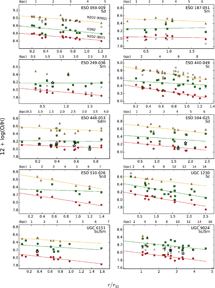
Figure 1: Radial O/H abundance gradients drawn in terms of the isophotal radius $r_{25}$ (lower scale of each panel) and of the physical radius in kpc (upper scale) from different diagnostics (see symbol explanation in the top left panel). In addition, star symbols are used for abundances obtained with the direct method (when available), and crosses for abundances from $R_{23}$ (only shown when branch selection is unambiguous). The lines represent least square fits to the abundance data. See text for explanations.

Table 4 and  5 summarize the slopes and zero points, respectively, of the metallicity gradients obtained when the nebular O/H values are based on the O3N2 and the N2O2 (B07) diagnostics. The slopes are reported, together with their errors, in terms of the physical size of the galaxies in kpc, of the isophotal radius $r_{25}$ and of the $B$-band exponential disc scale length $r_{d}$. We enclose these values in brackets when we wish to identify galaxies for which the errors exceed the absolute values of the slope, i.e. when the abundance gradient is formally consistent with a flat radial distribution. At the bottom of Table 4 we include the average slopes, with corresponding errors, and their standard deviations, calculated including all ten galaxies.

Before proceeding with the discussion, we make a few preliminary remarks, based on the results presented in Fig. 1 and Table 4:

1. a large fraction (50 per cent using the O3N2 diagnostic, 90 per cent using N2O2) of the sample galaxies present a significant radial abundance gradient The higher number of galaxies with gradients that are compatible with being flat in the case of O3N2 (5 out of 10) is related to the next point. Only one galaxy, ESO 187-051, has a flat gradient according to the N2O2 diagnostic.

2. In Fig. 1 the scatter of the data points corresponding to O3N2 (the mean rms of the linear fit is 0.095 dex) is approximately two times larger than for N2O2 (mean rms=0.044).

3. The slopes derived using O3N2 are either comparable to (within the errors) or shallower (ESO 249-036, ESO 440-049, ESO 510-026) than those obtained from N2O2. We interpret this difference and (ii) above with the higher dependence of O3N2 on the ionization parameter (e.g. Ho et al. 2015), and the fact that this diagnostic is constructed with both low- and high-excitation emission lines. While it is not immediately obvious why O3N2 should yield shallower gradients in some galaxies, we also point out that in absolute terms the difference in slope that can be obtained between the two diagnostics, while statistically significant, is small in our sample of galaxies in relation to the range of values found in much larger sample of spirals. Considering, for example, gradients in units of disc scale lengths the average slope from O3N2 is $-0.045\pm 0.013$ dex $r_{d}^{-1}$, compared to $-0.085\pm 0.010$ dex $r_{d}^{-1}$ from N2O2 (i.e. the difference is $\Delta_{O3N2-N2O2}=0.04$ dex $r_{d}^{-1}$). The slopes found by Sánchez et al. (2014) in a sample of 193 spiral galaxies (using O3N2) cover a much larger range, from $-0.19$ to $+0.04$ dex $r_{d}^{-1}$. Considering isophotal radii instead, the average slope from O3N2 is $-0.065\pm 0.018$ dex $r_{25}^{-1}$, compared to $-0.133\pm 0.024$ dex $r_{25}^{-1}$ from N2O2 ($\Delta_{O3N2-N2O2}=0.07$ dex $r_{25}^{-1}$). For the bulk of the 49 galaxies studied by Ho et al. (2015) using N2O2 the slope ranges from 0 to $-0.8$ dex $r_{25}^{-1}$. Therefore, the small systematic difference resulting from the selection of the abundance diagnostic does not hamper the comparison with the distribution of abundance gradient properties of HSBGs carried out in Sect.4.

4. In those cases where it has been possible to derive a reliable radial abundance trend also from $R_{23}$, we find results that are compatible either with N2O2 (all galaxies except ESO 249-036) or O3N2 (all galaxies except ESO 440-049).

For the reasons outlined in points (ii) and (iii) above, it is tempting to assign more significance to the results obtained from N2O2. For completeness, in the following discussion we will continue to consider gradients obtained from both O3N2 and N2O2.

Table 4: Abundance gradient slopes.

ID	O3N2						N2O2
	dex kpc-1	$\sigma$	dex $r_{25}^{-1}$	$\sigma$	dex $r_{d}^{-1}$	$\sigma$	dex kpc-1	$\sigma$	dex $r_{25}^{-1}$	$\sigma$	dex $r_{d}^{-1}$	$\sigma$
ESO 059-009	$-0.042$	0.020	$-0.165$	0.080	$-0.090$	0.044	$-0.040$	0.010	$-0.156$	0.039	$-0.085$	0.021
ESO 187-051	($+0.005$	0.023	$+0.019$	0.079	$+0.012$	0.051)	($-0.004$	0.010	$-0.014$	0.035	$-0.009$	0.022)
ESO 249-036	($+0.001$	0.040	$+0.001$	0.066	$+0.001$	0.070)	$-0.065$	0.018	$-0.108$	0.030	$-0.114$	0.031
ESO 440-049	$-0.013$	0.011	$-0.092$	0.076	$-0.036$	0.030	$-0.037$	0.005	$-0.256$	0.035	$-0.101$	0.014
ESO 446-053	($-0.006$	0.031	$-0.028$	0.138	$-0.015$	0.073)	$-0.023$	0.017	$-0.102$	0.074	$-0.054$	0.039
ESO 504-025	($-0.025$	0.028	$-0.063$	0.069	$-0.060$	0.065)	$-0.034$	0.011	$-0.086$	0.028	$-0.081$	0.026
ESO 510-026	($-0.009$	0.017	$-0.047$	0.087	$-0.019$	0.035)	$-0.047$	0.009	$-0.239$	0.047	$-0.097$	0.019
UGC 1230	$-0.022$	0.007	$-0.145$	0.043	$-0.099$	0.029	$-0.023$	0.004	$-0.149$	0.026	$-0.101$	0.018
UGC 6151	$-0.020$	0.017	$-0.082$	0.069	$-0.050$	0.042	$-0.039$	0.006	$-0.161$	0.026	$-0.098$	0.016
UGC 9024	$-0.015$	0.006	$-0.049$	0.020	$-0.092$	0.038	$-0.018$	0.004	$-0.059$	0.012	$-0.112$	0.022
Average	$-0.015$	0.004	$-0.065$	0.018	$-0.045$	0.013	$-0.033$	0.005	$-0.133$	0.024	$-0.085$	0.010
Standard dev.	- 0.013		- 0.055		- 0.038		- 0.016		- 0.072		- 0.030

The brackets are used to identify regressions for which the slope is flat within the quoted errors.

Table 5: Abundance gradient zero points.

ID	O3N2aaaaaa		N2O2
	12+log(O/H)	$\sigma$	12+log(O/H)	$\sigma$
ESO 059-009	8.796	0.054	8.607	0.025
ESO 187-051	8.256	0.076	8.052	0.033
ESO 249-036	8.181	0.071	8.046	0.032
ESO 440-049	8.543	0.062	8.434	0.029
ESO 446-053	8.227	0.075	8.122	0.040
ESO 504-025	8.439	0.105	8.263	0.043
ESO 510-026	8.355	0.080	8.255	0.043
UGC 1230	8.428	0.061	8.206	0.035
UGC 6151	8.339	0.052	8.098	0.019
UGC 9024	8.308	0.055	8.049	0.029

4 Discussion

The first finding of this work has already been introduced in the previous section: late-type (spiral) LSBGs do have measurable radial metallicity gradients. We thus do not confirm the earlier result by de Blok & van der Hulst (1998), who found no evidence for the presence of such gradients in LSBGs. The origin of this discrepancy can be attributed to a number of factors that are likely to affect their study: small sample size (three galaxies), galaxy morphology (irregulars), small number of H ii regions with limited radial coverage, and possibly the use of the $R_{23}$ diagnostic in the uncertain turnaround region. We believe that our result is robust, being based on a relatively large number of H ii regions per galaxy (up to 21), and on deeper spectra than was possible in the 1990’s.

Our study finally answers the question raised by Edmunds (1999), who speculated that the chemical evolution of low and high surface brightness galaxies should proceed in a similar fashion, and wondered whether LSBGs and HSBGs ‘might not show similar radial abundance gradients, since organization of star formation by spiral structure is a good candidate mechanism for gradient generation’. Indeed our observations show that, as in the case of HSBG spirals, metallicity gradients are a common characteristic of spiral LSBGs, implying that models of inside-out disc formation can explain the chemical abundance properties of these galaxies, too. It is not necessary to invoke drastically different modes of disc buildup for LSBGs, as suggested in the literature in order to account for the apparent lack of abundance gradients (de Blok & van der Hulst 1998; Vorobyov et al. 2009).

The question we wish to address next is whether the gradients observed in LSBGs are quantitatively comparable to those of HSBGs. For this purpose we compare the slopes obtained in Section 3 with those measured from large samples of HSBGs recently published by Sánchez et al. (2014) and Ho et al. (2015). Both studies confirm, with higher statistical significance, earlier findings obtained from smaller samples of galaxies and H ii regions (e.g. Vila-Costas & Edmunds 1992; Zaritsky, Kennicutt & Huchra 1994; Garnett et al. 1997), namely that spirals are characterized by similar abundance gradients, irrespective of morphological type and other global properties, when normalized to either the exponential disc scale length or the isophotal radius.

a) Sánchez et al. (2014) analyzed the abundance gradient properties of 306 galaxies observed as part of the Calar Alto Legacy Integral Field Area survey (CALIFA, Sánchez et al. 2012). Chemical abundances could be derived for at least four H ii regions per system in 193 galaxies, allowing a determination of their radial abundance gradients. These authors established the existence of a characteristic slope of the radial metallicity (O/H) gradient, that is independent of the properties of non-interacting, isolated galaxies, such as morphological type, presence of bars, and stellar mass. Considering only their subsample of 146 isolated galaxies, showing no evidence for ongoing interactions, the characteristic gradient, expressed in terms of the disc effective radius $r_{e}$, has a value $\alpha=-0.11$ dex $r_{e}^{-1}$, with a standard deviation of 0.08 dex $r_{e}^{-1}$. The normalized histogram of the slope distribution, extracted from Fig. 8 in Sánchez et al. (2014), is shown in the top panel of Fig. 2 by the black, dot-dashed line.

We can make a direct comparison with the average value we obtained for LSBGs using the O3N2 diagnostic, which was also adopted by Sánchez et al. (2014): $\alpha_{r_{d}}=-0.045\pm 0.038$ dex $r_{d}^{-1}$ (mean $\pm$ standard deviation), which translates into $\alpha_{r_{e}}=-0.076\pm 0.064$ dex $r_{e}^{-1}$ (accounting for the fact that $r_{e}=1.678\,r_{d}$). The distribution of the slope values we obtain for the LSBGs is shown in the top panel of Fig. 2 by the red, continuous line. It can be seen that the mean slopes for the HSBGs and LSBGs are indistinguishable, and that the two distributions are also compatible with each other, as confirmed by the $t$–test and the Kolgomorov–Smirnov test, respectively.

We note that, while the CALIFA sample analyzed by Sánchez et al. (2014) is complete only at the bright end, the luminosity of the 146 non-interacting galaxies that constitute our comparison sample extends down to $M_{g}\simeq-17$, thus overlapping with the luminosity range of the LSBGs in our sample. Moreover, the analysis by Sánchez et al. (2014) excluded trends of abundance gradient slopes with galaxy luminosity.

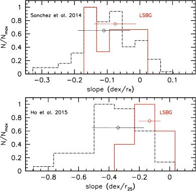
Figure 2: (Top) Histogram of the slope distribution for the LSBGs (red continuous line) and for the sample by Sánchez et al. (2014, black dot-dashed line). Units for the slope are dex $r_{e}^{-1}$. (Bottom) Histogram of the slope distribution for the LSBGs (red continuous line) and for the sample by Ho et al. (2015, black dot-dashed line). Units for the slope are dex $r_{25}^{-1}$. In both panels mean values (diamonds) and standard deviations (horizontal bars) are indicated for the different samples.

b) Ho et al. (2015) presented the metallicity gradient properties of 49 spiral galaxies with absolute magnitudes $-16>M_{B}>-22$ in the N2O2 (KD02) abundance scale. We note the good overlap in absolute magnitude with our LSBG sample. In the previous section we showed that when measuring gradient slopes, in alternative to the KD02 calibration, we can use the B07 calibration, with the results summarized in Table 4. Ho et al. (2015) found evidence for a common gradient among their galaxies, when the slope is expressed in units of the isophotal radius $r_{25}$. For the fainter half of their sample ($M_{B}>-20.1$), to which we compare our galaxies, they found a mean slope $\alpha_{r_{25}}=-0.34$ dex $r_{25}^{-1}$, with a standard deviation of 0.17 (for the full sample the slope is similar: $-0.39$ dex $r_{25}^{-1}$, with a standard deviation of 0.18). This compares to an average value $\alpha_{r_{25}}=-0.133$ dex $r_{25}^{-1}$ for our LSBG sample, with a standard deviation of 0.072. The bottom panel of Fig. 2 shows the distribution of the gradient slopes for the Ho et al. (2015) sample (black, dot-dashed line) and the LSBGs (red, continuous line).

The $t$–test indicates that in this case the difference between the average slopes of HSBGs and LSBGs is statistically significant ($p=0.0004$). A similar comparison with the HSBG sample presented by Pilyugin et al. (2014a), excluding galaxies in pairs or mergers, as discussed by Ho et al. 2015, yields the same conclusion.

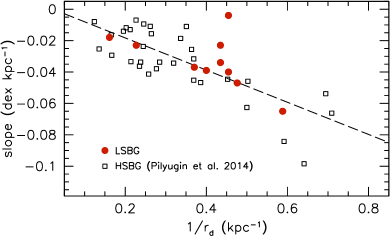
Figure 3: Slope of the abundance gradients, in dex kpc^-1, as a function of the $B$-band exponential disc scale length $r_{d}$ for our LSBGs (red full dots) and a sample of HSBGs (open squares; slopes from Pilyugin et al. 2014a and disc lengths from Pilyugin et al. 2014b).

4.1 Interpretation of the observed trends: clues on the common abundance gradients of spiral galaxies

We show in Fig. 3 the slope of the abundance gradients, now expressed in dex kpc^-1, as a function of the reciprocal of the $B$-band exponential disc scale length $1/r_{d}$ for our LSBGs (red full dots) and a sample of HSBGs for which the relevant information is readily available (open squares; slopes from Pilyugin et al. 2014a and disc lengths from Pilyugin et al. 2014b). The plot illustrates how LSBGs follow the same trend observed for HSBGs, namely that the gradient slope in dex kpc^-1 anticorrelates with galaxy size: large discs display shallower gradients compared to small discs. As suggested by Prantzos & Boissier (2000), who discussed a similar plot in their modeling of spiral galaxies as a function of the rotational velocity and spin parameter of their haloes, this trend describes a fundamental property of galaxy discs, since 1/$r_{d}$ measures the radial decrease of the surface brightness with radius in mag arcsec^-2 kpc^-1 [this follows from the equation for the exponential decrease of the surface brightness $\Sigma(r)=\Sigma(0)\exp(-r/r_{d})$ and the corresponding equation when using magnitudes $\mu(r)=\mu_{0}+1.086\,r/r_{d}$]. Our plot in Fig. 3 suggests that the underlying cause for the rate of radial decrease of the metallicity per kpc in discs is the same for all galaxies, regardless of their surface brightness. We argue that this is simply the rate of variation of the mass surface density with radius (also described by 1/$r_{d}$), through the local mass surface density–metallicity relation $\Sigma_{M}-Z$ (Edmunds & Pagel 1984; Rosales-Ortega et al. 2012; Moran et al. 2012), or equivalently the local stellar surface brightness–metallicity relation $\Sigma_{L}-Z$ (Ryder 1995; Pilyugin et al. 2014b). Smaller galaxies have a steeper slope (in dex kpc^-1) in the radial decrease of both the surface mass density (or surface luminosity) and metallicity. A linear least square fit to the data in Fig. 3 yields the following:

$$\frac{d\log(O/H)}{dr}=-0.102\,(\pm 0.014)\frac{1}{r_{d}}+0.002\,(\pm 0.005)$$ (1)

with distances expressed in kpc. Recalling that we can write $1/r_{d}=\Delta\mu/(1.086\Delta r)$ using the variation of the surface brightness between two points separated by a linear distance $\Delta r$, we can derive from Eq. (1) a simple relation between the change of $O/H$ and the corresponding variation in surface luminosity $\log\Sigma$:

$$\Delta\log(O/H)=0.235\,(\pm 0.032)\,\Delta\log\Sigma_{L_{B}}$$ (2)

From the same HSBG galaxies included in Fig. 3 Pilyugin et al. (2014b) determined that $\Delta\log(O/H)=0.286\,(\pm 0.090)\,\Delta\log\Sigma_{L_{B}}$ for the centers of spiral discs, which agrees with Eq. (2) within the errors. Relations with comparable coefficients, valid across the discs of spirals, were found by Ryder (1995), but for different photometric passbands (e.g. $0.237\pm 0.085$ in the $I$-band).

If the underlying mechanism is the same why, then, is the mean slope of the gradient of LSBGs shallower than for HSBGs, when expressed in terms of the isophotal radius $r_{25}$, but similar when referred to the exponential disc scale length, as shown above? Our interpretation, outlined below, is that the former result is due to a sort of selection effect, dependent on the disc central surface brightness. Our argument also explains the existence of a common abundance gradient slope for HSBGs, as confirmed by Sánchez et al. (2014) and others.

Let us consider abundance gradients expressed in terms of the isophotal radius, $r_{25}$. For a typical HSBG, we adopt the central surface brightness as given by the canonical Freeman (1970) value of $\mu_{B}(0)=21.65$ mag arcsec^-2. Across the isophotal radius, the surface brightness varies by $\Delta\mu_{{}_{\!\mbox{\tiny\rm HSBG}}}=25-21.65=3.35$ mag arcsec^-2. For a typical LSBG, we adopt instead $\mu_{B}(0)=23.2$ mag arcsec^-2 (the median value in Table 1, but this choice is somewhat arbitrary), and the variation over the isophotal radius is reduced to $\Delta\mu_{{}_{\!\mbox{\tiny\rm LSBG}}}=1.8$ mag arcsec^-2. Converting surface brightness to surface luminosity $\Sigma_{L}$ (e.g. measured in $L_{\odot}\,pc^{-2}$) the corresponding radial variations are ($\Delta\log\Sigma_{L})_{{}_{\!\mbox{\tiny\rm HSBG}}}=1.34$ and ($\Delta\log\Sigma_{L})_{{}_{\!\mbox{\tiny\rm LSBG}}}=0.72$. We assume now that the linear form of the local relation between log(O/H) and $\log\Sigma_{L}$ applies to all galaxies. We avoid the use of the local $\Sigma_{M}-Z$ relation, which requires an assumption about the mass-to-light ratio, and although these surface density–metallicity relations are better fit with second order polynomials (Rosales-Ortega et al. 2012) or using additional parameters (e.g. disc scale length or morphology, Pilyugin et al. 2014b), the intent of our estimate is simply to reproduce the essential trends.

Using Eq. (2) we can now estimate the variation of the O/H ratio across the isophotal radius $r_{25}$ to be $\Delta\log(O/H)_{{}_{\!\mbox{\tiny\rm HSBG}}}=0.31$ dex and $\Delta\log(O/H)_{{}_{\!\mbox{\tiny\rm LSBG}}}=0.17$ dex. These estimates compare well with the actual average measurements discussed above ($0.34$ and $0.13$ dex, respectively), and the small differences can easily be attributed both to the approximate nature of our calculations (including the choice of the central surface brightness for LSBGs) and the relatively large scatter in the observational data. We can conclude that LSBGs have a shallower mean abundance gradient in comparison to HSBGs, when expressed in terms of the isophotal radius, simply as a result of the reduced range in surface brightness measured between their centers and their isophotal radii. This effect is naturally not observed when the gradients are expressed in terms of the exponential disc scale length because over such a length the variations in surface brightness, surface luminosity and surface mass density are independent of the central surface brightness (e.g. the surface brightness decreases by a constant 1.086 magnitudes arcsec^-2 over this length).

A far-reaching corollary to these simple considerations is that the common abundance gradient slopes observed in HSBGs, expressed either in terms of disc scale lengths or isophotal radii (as found by Sánchez et al. 2014, Ho et al. 2015 and others), and their relatively small dispersions, derive naturally from the surface mass density (or luminosity)–metallicity relation (see also the discussion in Sánchez et al. 2014) and, in the case of the gradients per isophotal radii, the narrow range in central surface brightness spanned by the HSBGs typically selected for chemical abundance analysis. With a dispersion of 0.3 mag arcsec^-2 in $\mu_{B}(0)$ (Freeman 1970) and a dispersion of 0.11 dex in O/H coming from the empirical $\Sigma_{L}-Z$ relation (Pilyugin et al. 2014b) we roughly estimate a dispersion in the gradient slope of $\sim 0.12$ dex r${}_{25}^{-1}$, which compares well with $\sigma=0.12$ dex r${}_{25}^{-1}$ and $\sigma=0.18$ dex r${}_{25}^{-1}$ reported by Sánchez et al. (2014) and Ho et al. (2015), respectively. These figures can be improved with appropriate modeling of the uncertainties involved, but this lies beyond the scope of our study. Considering scale lengths instead, the mean value found in the $g$-band by Fathi et al. (2010) for a large sample of galaxies from the Sloan Digital Sky Survey is $3.85\pm 2.10$ kpc. Using Eq. (1) we derive a corresponding gradient of $\alpha=-0.15$ dex $r_{e}^{-1}$, with a standard deviation of 0.08 dex $r_{e}^{-1}$. There is a systematic offset in comparison with the average slope measured by Sánchez et al. (2014), but the standard deviation is the same.

Lastly, we conclude that the common abundance gradient measured in dex $r_{d}^{-1}$ expresses a more fundamental property of spiral discs than the common gradient in dex $r_{25}^{-1}$, being linked to the underlying physics (the existence of a local mass surface density–metallicity relation and its relative variations with radius) in a simpler way, without dependence on structural properties such as the actual value of the central mass surface density.

5 Summary

Our observations show that LSBGs have measurable radial chemical abundance gradients, qualitatively similar to those present in the more extensively studied high surface brightness galaxies. This result contrasts with the previously held notion that LSBGs do not possess such gradients. In addition, we found that the mean LSBG gradient, when expressed in terms of the isophotal radius, is significantly shallower than for the average HSBG. Since both LSBGs and HSBGs follow the same relation between the radial gradients of both metallicity (in dex kpc^-1) and surface brightness (in magnitudes  arcsec^-2 kpc^-1), we can explain this result simply adopting a common surface luminosity–metallicity relation (reflection of the more fundamental relation involving the mass surface density) and considering the range in surface brightness across the optical discs. The common gradient in dex r${}_{25}^{-1}$ observed in HSBGs derives from the similarity of their surface brightness (or equivalently mass surface density) gradients and central surface brightness. The latter conclusion does not contradict alternative explanations for the existence of this common abundance gradient. For example, Ho et al. (2015) based their interpretation on the similarity of the radial gas and stellar surface density profiles among spiral discs. Our reformulation, based on the structural similarity and the surface brightness properties, yields a concordant, equivalent interpretation. On the other hand, when normalizing the gradients to the exponential disc scale lengths we directly expose the underlying physical mechanism, i.e. the mass surface density–metallicity relation, and the homology with which it varies with galactocentric distance among galaxies.

References

- Asplund et al. (2009) Asplund M., Grevesse N., Sauval A. J., Scott P., 2009, ARA&A, 47, 481
- Auld et al. (2006) Auld R., de Blok W. J. G., Bell E., Davies J. I., 2006, MNRAS, 366, 1475
- Baldwin et al. (1981) Baldwin J. A., Phillips M. M., Terlevich R., 1981, PASP, 93, 5
- Beijersbergen et al. (1999) Beijersbergen M., de Blok W. J. G., van der Hulst J. M., 1999, A&A, 351, 903
- Bell et al. (2000) Bell E. F., Barnaby D., Bower R. G., de Jong R. S., Harper D. A., Hereld M., Loewenstein R. F., Rauscher B. J., 2000, MNRAS, 312, 470
- Bergmann et al. (2003) Bergmann M. P., Jørgensen I., Hill G. J., 2003, AJ, 125, 116
- Boissier et al. (2003) Boissier S., Monnier Ragaigne D., Prantzos N., van Driel W., Balkowski C., O’Neil K., 2003, MNRAS, 343, 653
- Boissier et al. (2008) Boissier S., et al., 2008, ApJ, 681, 244
- Bresolin (2007) Bresolin F., 2007, ApJ, 656, 186
- Bresolin et al. (2004) Bresolin F., Garnett D. R., Kennicutt R. C., 2004, ApJ, 615, 228
- Bresolin et al. (2009a) Bresolin F., Ryan-Weber E., Kennicutt R. C., Goddard Q., 2009a, ApJ, 695, 580
- Bresolin et al. (2009b) Bresolin F., Gieren W., Kudritzki R., Pietrzyński G., Urbaneja M. A., Carraro G., 2009b, ApJ, 700, 309
- Bresolin et al. (2010) Bresolin F., Stasińska G., Vílchez J. M., Simon J. D., Rosolowsky E., 2010, MNRAS, 404, 1679
- Bresolin et al. (2012) Bresolin F., Kennicutt R. C., Ryan-Weber E., 2012, ApJ, 750, 122
- Burkholder et al. (2001) Burkholder V., Impey C., Sprayberry D., 2001, AJ, 122, 2318
- Croxall et al. (2009) Croxall K. V., van Zee L., Lee H., Skillman E. D., Lee J. C., Côté S., Kennicutt Jr. R. C., Miller B. W., 2009, ApJ, 705, 723
- de Blok & van der Hulst (1998) de Blok W. J. G., van der Hulst J. M., 1998, A&A, 335, 421
- de Blok et al. (1995) de Blok W. J. G., van der Hulst J. M., Bothun G. D., 1995, MNRAS, 274, 235
- Edmunds (1999) Edmunds M. G., 1999, in Davies J. I., Impey C., Phillips S., eds, Astronomical Society of the Pacific Conference Series Vol. 170, The Low Surface Brightness Universe. p. 383
- Edmunds & Pagel (1984) Edmunds M. G., Pagel B. E. J., 1984, MNRAS, 211, 507
- Fathi et al. (2010) Fathi K., Allen M., Boch T., Hatziminaoglou E., Peletier R. F., 2010, MNRAS, 406, 1595
- Freeman (1970) Freeman K. C., 1970, ApJ, 160, 811
- Fu et al. (2013) Fu J., et al., 2013, MNRAS, 434, 1531
- Garnett et al. (1997) Garnett D. R., Shields G. A., Skillman E. D., Sagan S. P., Dufour R. J., 1997, ApJ, 489, 63
- Gerritsen & de Blok (1999) Gerritsen J. P. E., de Blok W. J. G., 1999, A&A, 342, 655
- Ho et al. (2015) Ho I.-T., Kudritzki R.-P., Kewley L. J., Zahid H. J., Dopita M. A., Bresolin F., Rupke D. S. N., 2015, MNRAS, 448, 2030
- Impey & Bothun (1997) Impey C., Bothun G., 1997, ARA&A, 35, 267
- Jones et al. (2013) Jones T., Ellis R. S., Richard J., Jullo E., 2013, ApJ, 765, 48
- Kewley & Dopita (2002) Kewley L. J., Dopita M. A., 2002, ApJS, 142, 35
- Kewley & Ellison (2008) Kewley L. J., Ellison S. L., 2008, ApJ, 681, 1183
- Kewley et al. (2010) Kewley L. J., Rupke D., Jabran Zahid H., Geller M. J., Barton E. J., 2010, ApJ, 721, L48
- Kobulnicky et al. (1999) Kobulnicky H. A., Kennicutt Jr. R. C., Pizagno J. L., 1999, ApJ, 514, 544
- Kudritzki et al. (2008) Kudritzki R.-P., Urbaneja M. A., Bresolin F., Przybilla N., Gieren W., Pietrzyński G., 2008, ApJ, 681, 269
- Kudritzki et al. (2012) Kudritzki R.-P., Urbaneja M. A., Gazak Z., Bresolin F., Przybilla N., Gieren W., Pietrzyński G., 2012, ApJ, 747, 15
- Kuzio de Naray et al. (2004) Kuzio de Naray R., McGaugh S. S., de Blok W. J. G., 2004, MNRAS, 355, 887
- Lauberts (1982) Lauberts A., 1982, ESO/Uppsala survey of the ESO(B) atlas. European Southern Observatory
- Lauberts & Valentijn (1989) Lauberts A., Valentijn E. A., 1989, The surface photometry catalogue of the ESO-Uppsala galaxies. European Southern Observatory
- Li et al. (2013) Li Y., Bresolin F., Kennicutt Jr. R. C., 2013, ApJ, 766, 17
- Liang et al. (2010) Liang Y. C., et al., 2010, MNRAS, 409, 213
- Longmore et al. (1982) Longmore A. J., Hawarden T. G., Goss W. M., Mebold U., Webster B. L., 1982, MNRAS, 200, 325
- López-Sánchez et al. (2012) López-Sánchez Á. R., Dopita M. A., Kewley L. J., Zahid H. J., Nicholls D. C., Scharwächter J., 2012, MNRAS, 426, 2630
- Makarov et al. (2014) Makarov D., Prugniel P., Terekhova N., Courtois H., Vauglin I., 2014, A&A, 570, A13
- Marino et al. (2012) Marino R. A., et al., 2012, ApJ, 754, 61
- Matthews & Gallagher (1997) Matthews L. D., Gallagher III J. S., 1997, AJ, 114, 1899
- McGaugh (1991) McGaugh S. S., 1991, ApJ, 380, 140
- McGaugh (1994) McGaugh S. S., 1994, ApJ, 426, 135
- McGaugh & Bothun (1994) McGaugh S. S., Bothun G. D., 1994, AJ, 107, 530
- McGaugh et al. (1995) McGaugh S. S., Schombert J. M., Bothun G. D., 1995, AJ, 109, 2019
- Moran et al. (2012) Moran S. M., et al., 2012, ApJ, 745, 66
- Nilson (1973) Nilson P., 1973, Uppsala general catalogue of galaxies. Stockholm: Almqvist & Wiksell (distr.)
- Patterson & Thuan (1996) Patterson R. J., Thuan T. X., 1996, ApJS, 107, 103
- Pettini & Pagel (2004) Pettini M., Pagel B. E. J., 2004, MNRAS, 348, L59
- Pilyugin et al. (2014a) Pilyugin L. S., Grebel E. K., Kniazev A. Y., 2014a, AJ, 147, 131
- Pilyugin et al. (2014b) Pilyugin L. S., Grebel E. K., Zinchenko I. A., Kniazev A. Y., 2014b, AJ, 148, 134
- Pilyugin et al. (2015) Pilyugin L. S., Grebel E. K., Zinchenko I. A., 2015, MNRAS, 450, 3254
- Prantzos & Boissier (2000) Prantzos N., Boissier S., 2000, MNRAS, 313, 338
- Queyrel et al. (2012) Queyrel J., et al., 2012, A&A, 539, A93
- Rich et al. (2012) Rich J. A., Torrey P., Kewley L. J., Dopita M. A., Rupke D. S. N., 2012, ApJ, 753, 5
- Rönnback & Bergvall (1995) Rönnback J., Bergvall N., 1995, A&A, 302, 353
- Rosales-Ortega et al. (2010) Rosales-Ortega F. F., Kennicutt R. C., Sánchez S. F., Díaz A. I., Pasquali A., Johnson B. D., Hao C. N., 2010, MNRAS, 405, 735
- Rosales-Ortega et al. (2012) Rosales-Ortega F. F., Sánchez S. F., Iglesias-Páramo J., Díaz A. I., Vílchez J. M., Bland-Hawthorn J., Husemann B., Mast D., 2012, ApJ, 756, L31
- Ryder (1995) Ryder S. D., 1995, ApJ, 444, 610
- Sánchez et al. (2012) Sánchez S. F., et al., 2012, A&A, 538, A8
- Sánchez et al. (2014) Sánchez S. F., et al., 2014, A&A, 563, A49
- Sánchez et al. (2015) Sánchez S. F., et al., 2015, A&A, 573, A105
- Schombert & McGaugh (2014) Schombert J., McGaugh S., 2014, Publ. Astron. Soc. Australia, 31, 36
- Stasińska et al. (2013) Stasińska G., Peña M., Bresolin F., Tsamis Y. G., 2013, A&A, 552, A12
- van den Hoek et al. (2000) van den Hoek L. B., de Blok W. J. G., van der Hulst J. M., de Jong T., 2000, A&A, 357, 397
- van der Hulst et al. (1993) van der Hulst J. M., Skillman E. D., Smith T. R., Bothun G. D., McGaugh S. S., de Blok W. J. G., 1993, AJ, 106, 548
- van Zee & Haynes (2006) van Zee L., Haynes M. P., 2006, ApJ, 636, 214
- Vila-Costas & Edmunds (1992) Vila-Costas M. B., Edmunds M. G., 1992, MNRAS, 259, 121
- Vorobyov et al. (2009) Vorobyov E. I., Shchekinov Y., Bizyaev D., Bomans D., Dettmar R., 2009, A&A, 505, 483
- Yuan et al. (2011) Yuan T.-T., Kewley L. J., Swinbank A. M., Richard J., Livermore R. C., 2011, ApJ, 732, L14
- Zaritsky et al. (1994) Zaritsky D., Kennicutt Jr. R. C., Huchra J. P., 1994, ApJ, 420, 87