WSU–HEP–XXYY

Selected recent results on charm hadronic decays from BESIII

Hajime Muramatsu

School of Physics and Astronomy
University of Minnesota, Minneapolis, Minnesota 55455, USA

I report BESIII preliminary results on:

1. Measurement of $\sigma(e^{+}e^{-}\to D\bar{D})$ at E${}_{\rm{cm}}=3.773$ GeV

2. Study of the $D\bar{D}$ production line shape near E${}_{\rm{cm}}=3.773$ GeV

3. The first observation of singly Cabibbo-suppressed decay, $D\to\omega\pi$

4. Measurement of ${\cal B}(D_{S}^{+}\to\eta^{\prime}X)$ and ${\cal B}(D_{S}^{+}\to\eta^{\prime}\rho^{+})$ .

PRESENTED AT

The 7th International Workshop on Charm Physics (CHARM 2015)
Detroit, MI, 18-22 May, 2015

1 Hadronic decays of charm mesons

Studies of hadronic decays of charm mesons play an important role in the understanding the weak interactions at the $c$-sector and provide inputs for the beauty physics. Two of samples accumulated by the BESIII detector [1] that are taken at E${}_{\rm{cm}}=3.773$ GeV and $4.009$ GeV are very useful to study decays of $D$ and $D_{S}^{\pm}$ mesons.

The former is the largest $e^{+}e^{-}$ annihilation sample in the world to date, $2.92$ fb^-1 [2], that is taken around the nominal mass of $\psi(3770)$ resonance which predominantly decays into a pair of $D$ mesons. The latter, consisting of $482$ pb^-1 [3], also produces a pair of $D_{S}^{+}D_{S}^{-}$ with a sizable production rate ($\sigma(e^{+}e^{-}\to D_{S}^{+}D_{S}^{-})\sim~{}269$ pb), providing a clean event environment to study decays of $D_{S}^{\pm}$.

In this proceeding, I report four preliminary measurements from the BESIII collaboration based on the above two $e^{+}e^{-}$ annihilation data. The first two results are studies about $D$-pair productions at the vicinity of the $\psi(3770)$ resonance, a measurement of observed $\sigma(e^{+}e^{-}\to D\bar{D})$ at E${}_{\rm{cm}}=3.773$ GeV and a study of Born-level line shape of $\sigma(e^{+}e^{-}\to D\bar{D})$. I then present the first observation of the singly Cabibbo-suppressed decays (SCSD), $D\to\omega\pi$, and end this report with the measurements of ${\cal B}(D_{S}^{+}\to\eta^{\prime}X)$ and ${\cal B}(D_{S}^{+}\to\eta^{\prime}\rho^{+})$.

2 $\sigma(e^{+}e^{-}\to D\bar{D})$ at E${}_{\rm{cm}}=3.773$ GeV

Measuring observed $\sigma(e^{+}e^{-}\to D\bar{D})$ allows us to estimate the number of $D\bar{D}$ pairs produced in our sample by using the integrated luminosity of the corresponding sample[2]. This can then be used to normalize the measured signal yields to obtain a branching fraction.

As done by the CLEO collaboration [4], we measure the observed cross section by a double-tag technique, pioneered by the MARK III Collaboration [5]. This takes advantage of the fact that $D$-meson production near the $\psi(3770)$ resonance is solely through $D\bar{D}$.

Reconstructing one $D$ meson in the pair provides a single-tag yield, $N_{ST}^{i}$, with a final state, $i$. We seek $9$ different final states: $D^{0}\to(K^{-}\pi^{+}$, $K^{-}\pi^{+}\pi^{0}$, $K^{-}\pi^{+}\pi^{+}\pi^{-})$, and $D^{+}\to(K^{-}\pi^{+}\pi^{+}$, $K^{-}\pi^{+}\pi^{+}\pi^{0}$, $K_{S}^{0}\pi^{+}$, $K_{S}^{0}\pi^{+}\pi^{0}$, $K_{S}^{0}\pi^{+}\pi^{+}\pi^{-}$, $K^{+}K^{-}\pi^{+})$. (Unless otherwise noted, charge conjugate modes are implied throughout this report.) The detail reconstruction criteria can be found in other BESIII publications, such as Ref. [6].

$N_{ST}^{i}$ can be written as $N_{ST}^{i}=N_{D\bar{D}}\cdot{\cal B}(D\to i)\cdot\epsilon_{i}$, where $N_{D\bar{D}}$ is the number of $D\bar{D}$ produced and $\epsilon_{i}$ is the reconstruction efficiency for the decay mode, $D\to i$. Similarly, one can have $N_{ST}^{j}=N_{D\bar{D}}\cdot{\cal B}(D\to j)\cdot\epsilon_{j}$. When the pair decays explicitly into two final states, $D\to i$ and $\bar{D}\to j$, we have $N_{DT}^{ij}=N_{D\bar{D}}\cdot{\cal B}(D\to i)\cdot{\cal B}(\bar{D}\to j)\cdot\epsilon_{ij}$. Here, $N_{DT}^{ij}$ is the double tag yield when we simultaneously reconstruct the two mesons in the final states of $i$ and $j$. $\epsilon_{ij}$ is the corresponding reconstruction efficiency. Solving these for $N_{D\bar{D}}$, one arrives at;

$$N_{D\bar{D}}=\frac{N_{ST}^{i}\cdot N_{ST}^{j}\cdot\epsilon_{ij}}{N_{DT}^{ij}\cdot\epsilon_{i}\cdot\epsilon_{j}}.$$

The observed cross section is readily obtained by dividing $N_{D\bar{D}}$ by the total integrated luminosity.

We obtain $N_{ST}^{i}$ from distributions of beam-constrained mass, $M_{\mathrm{BC}}$, defined as $M_{\mathrm{BC}}\equiv\sqrt{E^{2}_{\rm{beam}}-|\vec{p}_{D}|^{2}}$. Figure 1 shows fits to $M_{\mathrm{BC}}$ distributions based on singly tagged events for the $9$ different final states. We use a signal shape predicted by Monte Carlo (MC) simulation. Each of these are convoluted with a Gaussian to take into account a discrepancy in resolution between data and MC, while using an ARGUS background function [7] to represent the background component.

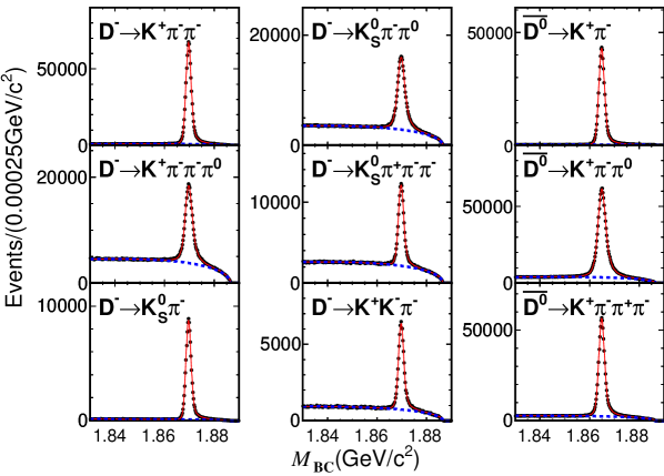
Figure 1: Fits to $M_{\mathrm{BC}}$ distributions of singly tagged events based on the entire $\psi(3770)$ sample. Red curves represent the overall fitted shapes and blue dashed curves correspond to the fitted ARGUS background functions.

As for obtaining $N_{DT}^{ij}$, we look at a two-dimensional space, $M_{\mathrm{BC}}^{i}$ vs $M_{\mathrm{BC}}^{j}$. Due to the small background of the doubly tagged events, we simply count the yields after using the sidebands of $M_{\mathrm{BC}}$ to estimate backgrounds.

Averaging the resultant observed cross sections over different final states ($D\to j$ and $\bar{D}\to j$ ), we have our preliminary result shown in Table 1. Our cross sections are consistent with the ones measured by the CLEO collaboration [4]. We expect our final results to be dominated by systematic uncertainties.

Experiment	$\sigma(e^{+}e^{-}\to D^{0}\bar{D^{0}})$ (nb)	$\sigma(e^{+}e^{-}\to D^{+}D^{-})$ (nb)
This work	$3.641\pm 0.010$	$2.844\pm 0.011$
CLEO [4]	$3.607\pm 0.017\pm 0.056$	$2.882\pm 0.018\pm 0.042$

Table 1: Comparison of the measured cross sections beween the BESIII preliminary results and the ones measured by the CLEO collaboration. Only statistical uncertainties are shown in the BESIII results.

3 Line shape of $\sigma(e^{+}e^{-}\to D\bar{D})$

In the previous section, I report our preliminary result of observed cross section, $\sigma(e^{+}e^{-}\to D\bar{D})$, at E${}_{\rm{cm}}=3.773$ GeV. It is of great interest to examine this production line shape near the nominal mass of $\psi(3770)$ resonance. This is done using the BESIII scan data which was taken in $2010$, along with the main on-resonant $\psi(3770)$ sample, in a range of $3.642<\rm{E}_{\rm{cm}}<3.890$ GeV with the total accumulated luminosity of $\sim 70$ pb^-1. Such a line shape distribution allows one to extract the $\psi(3770)$ resonance parameters. Table 2 shows some of the recent experimental measurements on the nominal mass of $\psi(3770)$ resonance. There is a definite (and expected) shift in the mass when an interference effect is taken into account.

Experiment	Mψ(3770) (MeV/$c^{2}$)
BES (2008) [8]	$3772.0\pm 1.9$
Belle (2008) [9]	$3776.0\pm 5.0\pm 4.0$
BABAR (2007) [10]${\dagger}$	$3778.8\pm 1.9\pm 0.9$
BABAR (2008) [11]	$3775.5\pm 2.4\pm 0.5$
KEDR (2012) [12]${\dagger}$	$3779.2^{+1.8+0.5+0.3}_{-1.7-0.7-0.3}$
${\dagger}$ includes interference

Table 2: Recent experimental measurements on the mass of the $\psi(3770)$ resonance.

To obtain the resonance parameters, we follow the procedure carried out by the KEDR collaboration [12] in which we assume that there are two sources that produce $D\bar{D}$ final states: one from the decay of $\psi(3770)$ and the other from non-$\psi(3770)$ decays. To represent the non-$\psi(3770)$ decays, we form its amplitude as a linear combination of a constant term, which represents the possible contributions from higher $c\bar{c}$ resonant states such as $\psi(4040)$, and a Breit-Wigner form, that corresponds to the $\psi(3686)$ tail above the $D\bar{D}$ mass threshold [13]. This approach is known as a Vector-Dominance Model (VDM), but we also try an exponential form, instead of the Breit-Wigner form, to see how much an alternate form affects the resultant $\psi(3770)$ resonance parameters.

The Born-level cross section, $\sigma_{born}$, and experimentally determined observed cross section, $\sigma_{obs}$, are related as:

$$\sigma_{obs}(W)=\int{z_{DD}(W\sqrt{1-x})\sigma_{born}(W\sqrt{1-x})F_{ISR}(x,W^{2})}dx.$$

Here, $z_{DD}$ is a factor for the coulomb interaction for $D^{+}D^{-}$, $F_{ISR}(x,W^{2})$ is the ISR radiator [14], and $G(W,W^{\prime})$ (a Gaussian) is there to take into account the beam spread at the initial E${}_{\rm{cm}}=W$. More details can be found in Ref. [12].

We extract $\sigma_{born}(W)$ based on $\sigma_{obs}(W)$ with the above relation. $\sigma_{obs}(W)$ is based on the singly tagged events by fitting to two-dimensional space, $\Delta E$ vs $M_{\mathrm{BC}}$, where $\Delta E\equiv E_{D}-E_{\rm{beam}}$ with both signal and background shapes are fixed based on MC samples. As an example, Fig. 2 shows projections onto the $M_{\mathrm{BC}}$ axes of such two-dimensional fits at E${}_{\rm{cm}}\sim 3.7735$ GeV (left) and E${}_{\rm{cm}}\sim 3.7984$ GeV (right) based on the sum of the three $D^{0}$ decays (see the $3^{rd}$ column of Fig. 1). Notice that the left plot of Fig. 2 peaks at nominal mass of $D^{0}$, while the right plot of Fig. 2 has a $2^{nd}$ peak on the higher side. This is due to the larger ISR effect at this particular E_cm, which our MC-based signal shape (green) reproduces quite well.

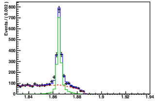
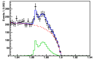
Figure 2: Projections onto the $M_{\mathrm{BC}}$ axes (in GeV/$c^{2}$) of the two-dimensional fits ($\Delta E$ vs $M_{\mathrm{BC}}$) at E${}_{\rm{cm}}\sim 3.7735$ GeV (left) and E${}_{\rm{cm}}\sim 3.7984$ GeV (right) based on the sum of the three $D^{0}$ decay modes. The blue histograms represent the overall fits, while dashed red and solid green histograms correspond to the fitted background and signal shapes, respectively.

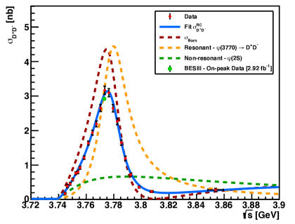
Figure 3: Observed cross section, $\sigma_{obs}$ is plotted in the red points based on the $D^{+}D^{-}$ events in which $D^{\pm}$ decays into the 6 different final states (see the $1^{st}$ and the $2^{nd}$ columns of Fig. 1). The corresponding $\sigma_{Born}$ curve is shown in dashed brown.

From these fits at each E_cm, we construct the spectrum of the observed cross section, $\sigma_{obs}$. As an example, we show $\sigma_{obs}$ distribution for the case of $D^{+}D^{-}$ (red points) in Fig 3. There, the solid blue curve is the fitted shape to $\sigma_{obs}$, while the corresponding $\sigma_{Born}$ is represented by the dashed brown curve. The dashed orange and green curves are the fitted resonant and non-resonant components (here, we use the VDM to represent the non-resonant component).

Table 3 shows our preliminary results on the nominal mass, total width, electronic partial width of the $\psi(3770)$ resonance. The $4^{th}$ column shows $\Gamma^{\psi(3770)}_{ee}\times{\cal B}_{D\bar{D}}$, where ${\cal B}_{D\bar{D}}={\cal B}(\psi(3770)\to D\bar{D})$. This is because our fit is only sensitive to the product of the two, but not individually. Our preliminary result is consistent with the KEDR measurement. In Tab. 3 we also show a result based on the exponential form to represent the non-$\psi(3770)$ amplitude. As can be seen, this would likely be one of the dominant sources of the systematic uncertainty.

Source	Mψ(3770) $($MeV/$c^{2})$	$\Gamma^{\psi(3770)}$ $($MeV$)$	$\Gamma^{\psi(3770)}_{ee}\times{\cal B}_{D\bar{D}}$ $($eV$)$
BESIIIVDM	$3781.5\pm 0.3$	$25.2\pm 0.7$	$230\pm 18$
BESIIIExponential	$3783.0\pm 0.3$	$27.5\pm 0.9$	$270\pm 24$
KEDR[12]	$3779.3^{+1.8}_{-1.7}$	$25.3^{+4.4}_{-3.9}$	$160^{+78}_{-58}$, $420^{+72}_{-80}$ (a)
PDG[15]	$3773.\pm 0.3$	$27.2\pm 1.0$	$[262\pm 18]\times{\cal B}_{D\bar{D}}$
(a) Two solutions were obtained from their fit.

Table 3: BESIII preliminary results based on the two different forms of the non-$\psi(3770)$ amplitudes, VDM ($\psi(3686)$) and an exponential shape, are shown, along with the result from the KEDR collaboration as well as the current PDG value. In the $4^{th}$ column, ${\cal B}_{D\bar{D}}={\cal B}(\psi(3770)\to D\bar{D})$.

4 $D\to\omega\pi$

For Cabibbo-suppressed charm decays, such as the yet to be observed SCSD $D\to\omega\pi$, measurements are difficult due to low signal statistics and high backgrounds. For the case of $D\to\omega\pi$, the most recent experimental search was carried out by the CLEO collaboration [16]. They set upper limits, ${\cal B}(D^{+}\to\omega\pi^{+})<3.0\times 10^{-4}$ and ${\cal B}(D^{0}\to\omega\pi^{0})<2.6\times 10^{-4}$ at $90\%$ confidence level (C.L.). In the mean time, H. Y. Cheng and C. W. Chiang predict the ${\cal B}(D\to\omega\pi)$ could be at an order of $1\times 10^{-4}$ [17].

We start with reconstructing one of the $D\bar{D}$ pairs with the same 9 final states (see Fig. 1). Then in the other $D$ decay, we look for $D^{+(0)}\to\omega\pi^{+(0)}$, where $\omega\to\pi^{+}\pi^{-}\pi^{0}$ and $\pi^{0}\to\gamma\gamma$. To improve the signal-to-noise ratio, we also select a certain range on the helicity-like angle of $\omega$, $\theta_{\rm{helicity}}$, which is defined as an opening angle between the direction of the normal to the $\omega\to\pi^{+}\pi^{-}\pi^{0}$ plane and the direction of the parent $D$ meson in the $\omega$ rest frame. We require $|H_{\omega}|=|\cos{\theta_{\rm{helicity}}}|>0.54(0.51)$ for $D^{+}$ ($D^{0}$) that are optimized based on a MC study.

With additional requirements on $M_{\mathrm{BC}}$ and $\Delta E$ to be consistent with a $D\bar{D}$ pair production, we extract our signal yields by fitting to the distributions of invariant mass of $\omega\to\pi^{+}\pi^{-}\pi^{0}$ as shown in Fig. 4. We use MC-based signal shapes, along with polynomials to represent their background shapes. Figure 4 also shows the expected peaking backgrounds (represented by filled histograms) which are estimated by the sidebands of $M_{\mathrm{BC}}$ distributions. The extracted signal yields correspond to a statistical significance of $5.4\sigma(4.1\sigma)$ for $D^{+}(D^{0})\to\omega\pi^{+}(\pi^{0})$, respectively.

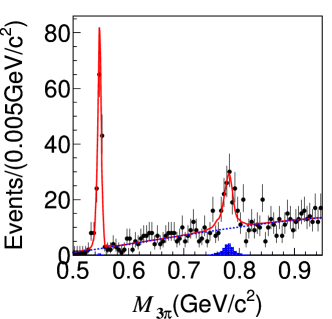
Figure 4: Distributions of invariant mass of $\omega\to\pi^{+}\pi^{-}\pi^{0}$ for $D^{+}\to\pi^{+}\pi^{-}\pi^{0}\pi^{+}$ (left) and $D^{0}\to\pi^{+}\pi^{-}\pi^{0}\pi^{0}$. The solid red lines are the overall fits, while the dashed blue lines represent the fitted polynomials The filled histograms represent the peaking backgrounds, estimated by the sidebands of $M_{\mathrm{BC}}$ distributions.

We also check to see if the $D\to\omega\pi$ candidates produce the expected distribution of the helicity angle. Figure 5 shows the distributions of $|H_{\omega}|$ in which we can see the expected $H^{2}_{\omega}=\cos^{2}\theta_{\rm{helicity}}$.

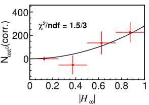
Figure 5: Efficiency-corrected signal yields in the $|H_{\omega}|$ bins for candidates of $D^{+}\to\omega\pi^{+}$ (left) and $D^{0}\to\omega\pi^{0}$ (right). The black lines are the fitted quadratic shapes.

In Fig. 4, we can also see peaks that correspond to $D\to\eta\pi$ candidates. We extract these candidates by fitting to the same invariant mass distributions of $\omega\to\pi^{+}\pi^{-}\pi^{0}$ with much narrower fit ranges, and without the requirement on the $|H_{\omega}|$. Figure 6 shows such fits from which we also measure ${\cal B}(D\to\eta\pi)$.

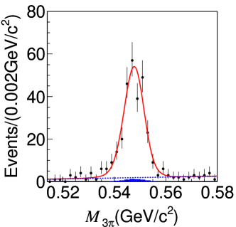
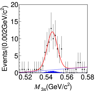
Figure 6: Fits to distributions of invariant mass of $\omega\to\pi^{+}\pi^{-}\pi^{0}$ for the candidates of $D^{+}\to\eta\pi^{+}$ (left) and $D^{0}\to\eta\pi^{0}$ (right). The filled histograms represent the peaking backgrounds which are estimated by the sideband regions of both signal and tag sides of $M_{\mathrm{BC}}$ distributions.

Table 4 shows our preliminary branching fraction measurements. The measured ${\cal B}(D\to\eta\pi)$ are consistent with the known values [15], while ${\cal B}(D\to\omega\pi)$ are measured for the first time.

Decay mode	This work	PDG value[15]
$D^{+}\to\omega\pi^{+}$	$(2.74\pm 0.58\pm 0.17)\times 10^{-4}$	$<3.4\times 10^{-4}$ at $90\%$ C.L.
$D^{0}\to\omega\pi^{0}$	$(1.05\pm 0.41\pm 0.09)\times 10^{-4}$	$<2.6\times 10^{-4}$ at $90\%$ C.L.
$D^{+}\to\eta\pi^{+}$	$(3.13\pm 0.22\pm 0.19)\times 10^{-4}$	$(3.53\pm 0.21)\times 10^{-3}$
$D^{0}\to\eta\pi^{0}$	$(0.67\pm 0.10\pm 0.05)\times 10^{-4}$	$(0.68\times 0.07)\times 10^{-3}$

Table 4: Preliminary result on the measured ${\cal B}(D\to\omega\pi)$.

5 $D_{S}^{+}\to\eta X$ and $D_{S}^{+}\to\eta\rho^{+}$

The situation of ${\cal B}(D_{S}^{+}\to\eta^{\prime}\rho^{+})$ is rather interesting. If we sum the all known exclusive rates with $\eta^{\prime}$ in $D_{S}^{+}$ decays in the PDG [15], we arrive at $(18.6\pm 2.3)\%$, while ${\cal B}(D_{S}^{+}\to\eta^{\prime}X)=(11.7\pm 1.7)\%$ [18]. Among the $D_{S}^{+}$ decays that involve $\eta^{\prime}$, the largest single exclusive rate is ${\cal B}(D_{S}^{+}\to\eta^{\prime}\rho^{+})=(12.5\pm 2.2)\%$ [19]. However, a recent measurement is about a half of it, ${\cal B}(D_{S}^{+}\to\eta^{\prime}\pi^{+}\pi^{0})=(5.6\pm 0.5\pm 0.6)\%$ [20] which appears to solve the inconsistency mentioned above. B. Bhattacharya and J. L. Rosner come up with two predictions, ${\cal B}(D_{S}^{+}\to\eta^{\prime}\rho^{+})=(2.9\pm 0.3)\%$ and $(1.89\pm 0.20)\%$ [21], while F. S. Yu et al. predict $(3.0\pm 0.5)\%$ [22] by factorization methods.

We can use our sample taken at E${}_{\rm{cm}}=4.009$ GeV to measure these branching fractions to confirm the recent measurement. At this energy, the $D_{S}^{\pm}$ is produced in a pair. To measure the inclusive rate, $D_{S}^{+}\to\eta^{\prime}X$, we employ a double-tag technique in which we reconstruct its tag side in $9$ decay modes shown in Fig. 7. From these $M_{\mathrm{BC}}$ distributions, the single-tag yields are readily obtained.

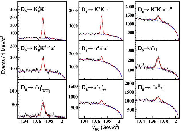
Figure 7: Fits to $M_{\mathrm{BC}}$ distributions of the selected $9$ different final states of $D_{S}^{+}$ decays. The red curves correspond to the total fits, while the blue dashed curves represent the fitted background shapes by the ARGUS background functions [7].

To obtain the double-tag yields, we reconstruct the $9$ final states of $D_{S}^{+}$ decays and look for the other $D_{S}^{\mp}$ decays in the final states with $\eta^{\prime}\to\pi^{+}\pi^{-}\eta(\to\gamma\gamma)$ based on the remaining particles. If there is more than one $\eta^{\prime}$ candidate, we choose the one that gives the minimum $|M_{\pi^{+}\pi^{-}\eta}-M_{\eta^{\prime}}(PDG)|$. We fit to a two-dimensional space, $M_{\pi^{+}\pi^{-}\eta}$ vs $M_{\mathrm{BC}}$, to extract the signal yields, where $M_{\mathrm{BC}}$ is the tag side of the beam-constrained mass. Figure 8 shows such fits, projected onto the $M_{\mathrm{BC}}$ axis (left) and onto the $M_{\pi^{+}\pi^{-}\eta}$ axis (right). We use MC-based distributions to represent the signal shape. As for the background shapes, an ARGUS background function [7] is used on the $M_{\mathrm{BC}}$ direction, while the smooth and peaking backgrounds on the $M_{\pi^{+}\pi^{-}\eta}$ axis are represented by a polynomial plus double Gaussian shapes.

From this fit, $68\pm 14$ events are observed as signal candidates. This translates into ${\cal B}(D_{S}^{+}\to\eta^{\prime}X)=(8.8\pm 1.8\pm 0.5)\%$ which agrees with the known value [15].

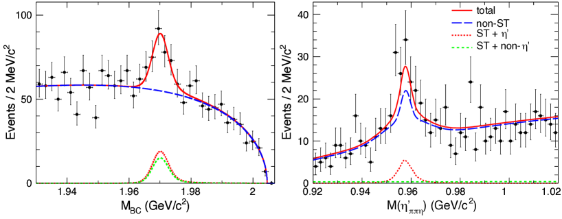
Figure 8: Fit to two-dimensional space, $M_{\pi^{+}\pi^{-}\eta}$ vs $M_{\mathrm{BC}}$, where $M_{\mathrm{BC}}$ is the tag side of the beam-constrained mass. Shown here are the fitted result, projected onto the $M_{\mathrm{BC}}$ axis (left) and onto the $M_{\pi^{+}\pi^{-}\eta}$ axis (right). Solid red curves correspond to the overall fit, while dashed blue and green curves are fitted peaking backgrounds.

To measure ${\cal B}(D_{S}^{+}\to\eta^{\prime}\rho^{+})$, we simply use the single-tag method by reconstructing $D_{S}^{+}\to\eta^{\prime}\rho^{+}$, where $\rho^{+}\to\pi^{+}\pi^{0}$. We require the reconstructed $\eta^{\prime}$ mass to be within $3\sigma$ of the known mass [15], the invariant mass $M_{\pi^{+}\pi^{0}}$ be within $0.17$ GeV/$c^{2}$ of the known $\rho$ mass [15], and finally its $\Delta E$ be consistent with zero.

The signal yield is extracted by fitting to two-dimensional space, $M_{\mathrm{BC}}$ vs $\cos\theta_{\pi^{+}}$, where $\theta_{\pi^{+}}$ is the helicity angle of the $\pi^{+}$ from the $\rho$ decay. We expect to see $\cos^{2}\theta_{\pi^{+}}$ for $D_{S}^{+}\to\eta^{\prime}\rho^{+}$, while $D_{S}^{+}\to\eta^{\prime}\pi^{+}\pi^{0}$ events should be independent of $\theta_{\pi^{+}}$.

Figure 9 shows projections onto the $M_{\mathrm{BC}}$ axis (left) of such two dimensional fit. On the right, a projection onto the $\cos\theta_{\pi^{+}}$ axis with an additional requirement of $(1.960<M_{\mathrm{BC}}<1.980)$ GeV/$c^{2}$ is shown. Signal shapes are based on MC simulation. To represent the background shapes, an ARGUS background function [7] is used on the $M_{\mathrm{BC}}$ axis, while a fixed non-$D_{S}^{+}$ background shape is employed on the $\cos\theta_{\pi^{+}}$ axis, estimated from the $M_{\mathrm{BC}}$ sidebands.

The fit yields $210\pm 50$ and $-13\pm 56$ events for $D_{S}^{+}\to\eta^{\prime}\rho^{+}$ and $D_{S}^{+}\to\eta^{\prime}\pi^{+}\pi^{0}$ candidates, respectively. We normalize the rate by $D_{S}^{+}\to K^{+}K^{-}\pi^{+}$ mode to obtain ${\cal B}(D_{S}^{+}\to\eta^{\prime}\rho^{+})/{\cal B}(D_{S}^{+}\to K^{+}K^{-}\pi^{+})=1.04\pm 0.25\pm 0.07$. Or with the known ${\cal B}(D_{S}^{+}\to K^{+}K^{-}\pi^{+})$ [15], we arrive at ${\cal B}(D_{S}^{+}\to\eta^{\prime}\rho^{+})=(5.8\pm 1.4\pm 0.4)\%$ which confirms the recent measurement by the CLEO collaboration [20]. We also set an upper limit on the non-resonant decay, ${\cal B}(D_{S}^{+}\to\eta^{\prime}\pi^{+}\pi^{0})<5.1\%$ at $90\%$ C.L.

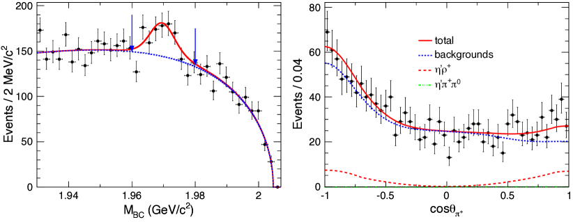
Figure 9: Projections onto the $M_{\mathrm{BC}}$ axis (left) and the $\cos\theta_{\pi^{+}}$ axis with an additional requirement of $(1.960<M_{\mathrm{BC}}<1.980)$ GeV/$c^{2}$ (right) of the two-dimensional fit.

6 Conclusion

Four preliminary results on the hadronic final states in the decays of $D$ and $D_{S}^{\pm}$ mesons based on the two recent BESIII samples are reported. The measurements based on the world’s largest $e^{+}e^{-}$ annihilation sample taken at E${}_{\rm{cm}}=3.773$ GeV provide statistically superior results than the previous experimental results, while the study of decays of $D_{S}^{\pm}$ based on the sample at E${}_{\rm{cm}}=4.009$ GeV shows the very clean event environment at BESIII. It would be very exciting to pursue our $D_{S}$ program as the collaboration plans to take a few fb^-1 of $e^{+}e^{-}$ annihilation sample at E${}_{\rm{cm}}=4.180$ GeV in $2015-2016$, where the production rate of $D_{S}^{\pm}$ is much higher, $\sigma(e^{+}e^{-}\to D_{S}^{*\pm}D_{S}^{\mp})\sim 900$ pb.

ACKNOWLEDGEMENTS

I would like to thank Derrick Toth, Andy Julin, Xiaoshuai Qin, and Peilian Liu for preparing and providing the figures and comments.

References

- [1] M. Ablikim et al. (BESIII Collaboration), Nucl. Instrum. Methods Phys. Res., Sec. A 614, 345 (2010).
- [2] M. Ablikim et al. (BESIII Collaboration), Chin. Phys. C 37, 123001 (2013).
- [3] M. Ablikim et al. (BESIII Collaboration), Chin. Phys. C 39, 093001 (2015).
- [4] G. Bonvicini et al. (CLEO Collaboration), Phys. Rev. D 89, 072002 (2014).
- [5] R. M. Baltrusaitis et al. (MARK III Collaboration), Phys. Rev. Lett. 56, 2140 (1986).
- [6] M. Ablikim et al. (BESIII Collaboration), Phys. Lett. B 744, 339 (2015).
- [7] H. Albrecht et al. (ARGUS Collaboration), Phys. Lett. B 241, 278 (1990).
- [8] M. Ablikim et al. (BES Collaboration), Phys. Lett. B 600, 315 (2008).
- [9] J. Brodzicka et al. (Belle Collaboration), Phys. Rev. Lett. 100, 092001 (2008).
- [10] B. Aubert et al. (BABAR Collaboration), Phys. Rev. D 76, 111105(R) (2007).
- [11] B. Aubert et al. (BABAR Collaboration), Phys. Rev. D 77, 011102(R) (2008).
- [12] V.V. Anashin et al. (KEDR Collaboration), Phys. Lett. B 711, 292 (2012).
- [13] Hai-Bo Li, Xiao-Shuai Qin, and Mao-Zhi Yang, Phys. Rev. D 81, 011501(R) (2010); Yuan-Jiang Zhang and Qiang Zhao, Phys. Rev. D 81, 034011 (2010).
- [14] E.A. Kuraev, V.S. Fadin, Sov. J. Nucl. Phys. 41, 466 (1985).
- [15] K. A. Olive et al. (Particle Data Group), Chin. Phys. C 37, 090001 (2014).
- [16] P. Rubin et al. (CLEO Collaboration), Phys. Rev. Lett. 96, 081802 (2006).
- [17] Hai-Yang Cheng and Cheng-Wei Chiang, Phys. Rev. D 81, 074021 (2010).
- [18] S. Dobbs et al. (CLEO Collaboration), Phys. Rev. D 79, 112008 (2009).
- [19] C. P. Jessop et al. (CLEO Collaboration), Phys. Rev. D 58, 052002 (1998).
- [20] P. U. E. Onyisi et al. (CLEO Collaboration), Phys. Rev. D 88, 032009 (2013).
- [21] B. Bhattacharya and J. L. Rosner, Phys. Rev. D 79, 034016 (2009).
- [22] Fu-Sheng Yu, Xiao-Xia Wang, and Cai-Dian Lü, Phys. Rev. D 84, 074019 (2011).