The Panchromatic Hubble Andromeda Treasury VIII: A Wide-Area, High-Resolution Map of Dust Extinction in M31

Abstract

We map the distribution of dust in M31 at $25{\rm\,pc}$ resolution, using stellar photometry from the Panchromatic Hubble Andromeda Treasury survey. The map is derived with a new technique that models the near-infrared color-magnitude diagram (CMD) of red giant branch (RGB) stars. The model CMDs combine an unreddened foreground of RGB stars with a reddened background population viewed through a log-normal column density distribution of dust. Fits to the model constrain the median extinction, the width of the extinction distribution, and the fraction of reddened stars in each $25{\rm\,pc}$ cell. The resulting extinction map has a factor of $\gtrsim$4 times better resolution than maps of dust emission, while providing a more direct measurement of the dust column. There is superb morphological agreement between the new map and maps of the extinction inferred from dust emission by Draine et al. (2014). However, the widely-used Draine & Li (2007) dust models overpredict the observed extinction by a factor of $\sim\!2.5,$ suggesting that M31’s true dust mass is lower and that dust grains are significantly more emissive than assumed in Draine et al. (2014). The observed factor of $\sim\!2.5$ discrepancy is consistent with similar findings in the Milky Way by Plank Collaboration et al. (2014), but we find a more complex dependence on parameters from the Draine & Li (2007) dust models. We also show that the discrepancy with the Draine et al. (2014) map is lowest where the current interstellar radiation field has a harder spectrum than average. We discuss possible improvements to the CMD dust mapping technique, and explore further applications in both M31 and other galaxies.

1. Introduction

Dust plays an increasingly important role in extragalactic astronomy. It has long been known that dust shapes the observational properties of disk galaxies, particularly in the optical and ultraviolet (e.g., Disney et al., 1989; Xilouris et al., 1999; Misiriotis et al., 2001; Pierini et al., 2004; Tuffs et al., 2004; Möllenhoff et al., 2006; Driver et al., 2007; Bianchi, 2008; Popescu et al., 2011). However, over recent decades, dust has become a wide-spread source of study in its own right (Savage & Mathis, 1979; Draine, 2003), thanks in large part to observational facilities that directly probe emission from the dust in the mid- and far-infrared, and at sub-millimeter wavelengths. This emission has also become a widely used tracer of key astrophysical quanitites, including the star formation rate and the interstellar radiation field (see review by Kennicutt & Evans, 2012).

Dust has also emerged as one of the most effective tracers of cold, dense gas. Molecular gas and cold Hi are the immediate precursors to star formation (see, for example Bergin & Tafalla, 2007; McKee & Ostriker, 2007; Hennebelle & Falgarone, 2012), and the properties of this gas is likely to be coupled to the ability of the interstellar medium (ISM) to form stars. Unfortunately, these cold gas components are extremely difficult to trace. Cold molecular hydrogen is nearly impossible to see in emission, and cold atomic Hi cannot be reliably distinguished from warmer phases without absorption line techniques.

The study of cold, dense gas has been fundamentally changed by the widespread use of dust extinction as a tracer (Lilley, 1955; Dickman, 1978; Frerking et al., 1982). Methods that used star counts to identify dust extinction had been in use for many years (e.g., Dickman, 1978; Cernicharo & Bachiller, 1984; Cambrésy et al., 1997; Cambrésy, 1999; Arce & Goodman, 1999; Dobashi et al., 2005, among many others), but were gradually supplanted by new methods taking advantage of the growing availability of near-infrared imaging, particularly due to the all-sky 2MASS (Skrutskie et al., 2006) and the UKIDSS/Galactic Plane (Lucas et al., 2008) surveys. Many groups have developed optimized methodologies to use near-infrared (NIR) color-color (or color-magnitude) diagrams (e.g., Lada et al., 1994; Ciardi et al., 1998; Lombardi & Alves, 2001; Cambrésy et al., 2002; Lombardi, 2005; Froebrich & del Burgo, 2006; Lombardi, 2009; Gonzalez et al., 2011) to identify molecular clouds in the Milky Way and to map their structure (Ciardi et al., 1998; Alves et al., 1998; Lada et al., 1999; Alves et al., 2001; Cambrésy et al., 2002; Teixeira et al., 2005; Lombardi et al., 2006; Froebrich et al., 2007; Lombardi et al., 2008; Kainulainen et al., 2009; Rowles & Froebrich, 2009; Lombardi et al., 2010; Román-Zúñiga et al., 2010; Frieswijk & Shipman, 2010; Scandariato et al., 2011; Dobashi, 2011; Kainulainen et al., 2011a, b; Gonzalez et al., 2012; Alves et al., 2014; Schlafly et al., 2015, and many others), with even more recent work using mid-infrared observations to map even denser clouds (Vasyunina et al., 2009; Butler & Tan, 2009; Majewski et al., 2011; Butler & Tan, 2012; Nidever et al., 2012; Kainulainen & Tan, 2013), and other work looking to exploit growing optical databases (e.g., Sale et al., 2009). The resulting maps are likely to be more direct tracers of the total column density than methods based on dust or molecular emission (e.g., Goodman et al., 2009).

The impact of extinction mapping can easily be seen in the diversity of problems they have been used to address. These maps have been used: to measure the statistics of the column density distribution (e.g., Lada et al., 1999; Kainulainen et al., 2009; Lombardi et al., 2010; Froebrich & Rowles, 2010; Schneider et al., 2011; Alves et al., 2014) and its connection to star formation (Lada et al., 2009; Rowles & Froebrich, 2011; Kainulainen et al., 2011b; Stutz & Kainulainen, 2015); to explore the origins of “Larson’s Laws” (Kauffmann et al., 2010; Lombardi et al., 2010; Beaumont et al., 2012; Ballesteros-Paredes et al., 2012); to measure the cloud structure function and clump statistics (e.g., Padoan et al., 2002, 2003; Kirk et al., 2006; Lombardi et al., 2008, 2010; Kauffmann et al., 2010); to study individual molecular cores and globules (e.g., Teixeira et al., 2005; Román-Zúñiga et al., 2009; Racca et al., 2009; Schmalzl et al., 2010); to constrain the relationship between dust column density and emission from molecular gas (e.g., Lada et al., 1994; Hayakawa et al., 2001; Harjunpää et al., 2004; Lombardi et al., 2006; Kainulainen et al., 2006; Pineda et al., 2010); to distinguish among models of turbulence (Padoan et al., 1997; Federrath et al., 2010; Kainulainen & Tan, 2013); to derive the 3-dimensional structure of the ISM (e.g., Sale & Magorrian, 2014; Schlafly et al., 2015; Green et al., 2015); and to constrain models of the dust itself (e.g., Roy et al., 2013).

Extinction mapping has also become a routine tool in the study of external galaxies. The Magellanic Clouds are sufficiently close to apply similar mapping techniques using NIR colors of individual stars (e.g., Dobashi et al., 2008, 2009), although their low extinctions allows optical and ultraviolet data to be used as well (e.g., Harris et al., 1997; Zaritsky et al., 2002, 2004). At larger distances, where individual stars can no longer be resolved, extinction maps are typically based on modeling the spectral energy distribution in individual pixels (e.g., Zibetti et al., 2009), but usually only as a way to removing the effects of dust, rather than as a route to studying the cold ISM itself.

In this paper, we focus on using M31 to bridge these two regimes. Andromeda is close enough that we can probe the ISM on the scales of molecular clouds. However, thanks to the large area covered by the Panchromatic Hubble Andromeda Treasury (PHAT; Dalcanton et al., 2012), we can also cover large areas, allowing us to view the entire cold ISM, rather than just individual clouds. This approach gives us our first view of the statistical properties of molecular clouds across a large fraction of a massive spiral galaxy.

Thanks to its proximity, M31 has been the target of many previous dust studies, including surveys of dust emission using space-based mid- and far-infrared (FIR) imagers on board IRAS (Devereux et al., 1994), Spitzer (Barmby et al., 2006; Gordon et al., 2006), and Herschel (Fritz et al., 2012; Groves et al., 2012). These observations have elucidated star formation, dust heating, the dust-to-gas ratio, and dust composition (e.g., Ford et al., 2013; Montalto et al., 2009; Tabatabaei & Berkhuijsen, 2010; Leroy et al., 2011; Groves et al., 2012; Smith et al., 2012; Draine et al., 2014), particularly when complemented by direct studies of the cold ISM in Hi (Brinks & Bajaja, 1986; Braun et al., 2009; Chemin et al., 2009) and CO (Nieten et al., 2006; Rosolowsky et al., 2007; Tosaki et al., 2007, though the latter two cover limited area).

Some of these studies have used the dust emission and other tracers to derive extinction maps (e.g., Montalto et al., 2009; Draine et al., 2014). Most recently, Draine et al. (2014) used mid- and far-infrared data to derive dust column densities throughout M31. These maps use state of the art models of dust to derive the spatial distribution of dust composition, heating, and dust column density. The models also make specific predictions for the extinction within M31.

In this paper we introduce a technique for probing the cold dusty ISM. We take advantage of the Panchromatic Hubble Andromeda Treasury’s (PHAT; Dalcanton et al., 2012) large database of NIR HST observations, and use photometry of individual RGB stars to derive the distribution of dust extinction on 25${\rm\,pc}$ scales. Specifically, we use the structure of the RGB seen in NIR color-magnitude diagrams (CMDs) to fit for the distribution of extinctions along the line of sight. The methodology therefore gives us both the median extinction and the width of the extinction distribution in each resolution element (pixel).

In Sec. 2 we give an overview of this technique, and explain its connection to observations of molecular clouds in the Milky Way. In Sec. 3 we derive the expected distribution of color and/or reddening for a log-normal distribution of dust embedded in thicker stellar disk. In Sec. 4, we give details of how we fit the parameters of the dust$+$star model to data from the PHAT survey, and discuss the distribution and accuracy of the derived parameters in Sec. 5. We show the global dust extinction map and compare it to the extinction inferred from fits to dust emission Sec. 6. We then conclude in Sec. 7.

2. Overview of Measuring Extinction with CMDs

Mapping extinction in the Milky Way requires coping with the complex distribution of both dust and stars along the line of sight. In external galaxies, however, the spread in distance is negligible, and all stars can be assumed to be at the same distance. This difference allows the full color and magnitude distribution of stars to be used when constructing extinction maps.

The impact of dust can be most easily perceived in the NIR CMD, which is populated almost entirely with RGB stars that occupy a small range of intrinsic color at given magnitude. Theoretically, the RGB should form a narrow, nearly vertical sequence in a NIR CMD. Empirically, however, the CMD structure of the RGB is complex and spatially varying, as shown in Figure 1. In many regions of M31, the NIR RGB is quite thin (as seen later in Figure 9), but in other regions it appears broad, and in some cases even bimodal. The broadening and/or bimodality is always seen redward of the thinner, bluer component, the latter of which always stays in essentially the same place on the CMD. Given that the color distribution of the bimodal RGB is not sensible in any stellar population model, and that the unusual morphologies change rapidly over very short distances, the natural explanation for the effects seen in Figure 1 is dust.

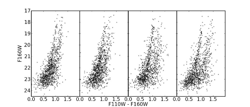
Figure 1.— The spatial variation in the NIR color magnitude diagrams, shown in 4 adjacent $20\arcsec$ bins within the disk of M31. Each CMD is dominated by red giant branch stars. There is a narrow, bluer RGB sequence that is similar in all regions, but that is accompanied by a highly variable redder RGB sequence, which varies in both width and position. RGB stars trace a sufficiently old stellar population that they should be well mixed at these spatial scales. The spatial variation in the redder population is therefore best explained by spatial variation in the dust that is obscuring some fraction of the RGB stars.

The CMD morphology in Figure 1 can be explained as follows. The thinner, bluer RGB sequence is due to old or intermediate age stars seen in front of the cool dusty ISM. The redder stars are then those that lie behind the layer of dust. The cool ISM is highly structured, and thus we see rapid small-scale spatial variations in the behavior of the reddened stars. Based upon this interpretation, we developed a method to simultaneously fit the unreddened and reddened stars to derive the distribution of dust extinction, which we describe in detail in Secs. 3 & 4.

At its heart, the method is based on recognizing that the RGB stars are point-like “samples” of the column density distribution function of the dust. We demonstrate this effect in Figure 2. The first panel shows a 2MASS-based extinction map of the Orion molecular cloud, kindly provided by J. Kainulainen (Kainulainen et al., 2009). We have adjusted the angular scale of the map to be consistent with being located at the distance of M31. The grid on the image indicates regions $25{\rm\,pc}$ across, which is the scale we use in our analysis below. The second panel shows the distribution of extinctions within each of these grid regions. In the PHAT NIR photometry, there are typically $\sim$100 RGB stars that fall within a region this size, and 20–80% of them lie behind the dust. The RGB stars therefore sample the dust structure on scales below that of the $25{\rm\,pc}$ grid, and even adjacent RGB stars may fall on regions with quite different extinctions.

If we assume that any stars coincident with regions in Figure 2 are primarily found in a stellar disk that is significantly thicker than the cool ISM (consistent with the high velocity dispersion of $\sim\!90{\rm\,km\,s^{-1}}$ seen in RGB stars; Dorman et al., 2015), some fraction of the stars will be behind the dust layer, with the exact fraction depending on the disk geometry. These stars will be reddened, and will sample the local distribution of reddening in the molecular cloud. By analyzing the reddening distribution, we can infer the statistical properties of the extinction distribution of the gas layer that they lie behind, for a given choice of extinction law. The same approach applies for any dusty gas layer, not just the densest regions identified as molecular clouds, as long as the amount of reddening is large enough to produce a measurable shift in the RGB.

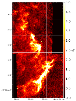
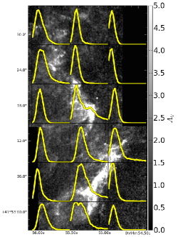
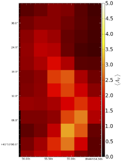
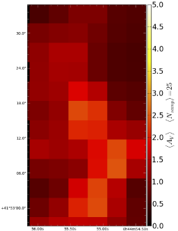
Figure 2.— Simulation of sampling the extinction distribution of the Orion molecular cloud at the distance of M31. (First Panel) The extinction map of Orion from Kainulainen et al. (2009), with the angular scale adjusted to place it at the distance of M31, and the RA and Dec shifted to a location in M31’s $10{\rm\,kpc}$ star-forming ring. Grid lines are 25${\rm\,pc}$ ($=6.645\arcsec$ apart). (Second Panel) The distribution of extinctions within each grid region (yellow), superimposed on the map from the top left. The same range of extinction is shown in each panel ($0<A_{V}<5{\rm\,mag}$). The distribution of extinctions can be reasonably characterized as a log-normal distribution in most cases. (Third Panel) The mean extinction, calculated using a dithered grid of 25${\rm\,pc}$, in steps of 12.5${\rm\,pc}$. In spite of the low resolution, the basic structure of the molecular cloud is still clearly visible. (Fourth Panel) The mean extinction in the same grid as in the lower left panel, but now calculated using only $\sim$25 randomly sampled pixels from the high resolution left-hand image in each 25${\rm\,pc}$ bin. Even this modest number of samples is sufficient to capture the same morphology seen in the middle panel, with a slight tendency to miss some of the highest extinctions.

As an example, the third panel of Figure 2 shows the mean extinction calculated in $25{\rm\,pc}$ bins (i.e, the same width as the grid lines in the upper panels), if the same region of the Orion molecular cloud shown in the upper panels were observed in M31; this bin size matches the fiducial bin size used in our analysis below, and provides a good balance between ensuring a large number of stars per bin, and maximizing resolution. To improve the spatial sampling of the distribution, we calculate the mean in 4 different grids, each shifted by half of a $25{\rm\,pc}$ pixel, and then interleave them into a grid with $12.5{\rm\,pc}$ pixels. The resulting map of the mean extinction clearly traces the same structure as the actual molecular cloud, albeit with lower resolution. The dynamic range is reduced because we are tracing the mean, and not the extremes of the distribution, and are convolving the data over the scale of a pixel.

The fourth panel of Figure 2 shows the same calculation of the mean extinction, but instead of averaging all the points in the original image, we use only averages from randomly selected lines of sight, which were laid down with an average spatial density of $\sim\!25$ samples per $25{\rm\,pc}$ bin (i.e., equivalent to what would be observed for an equivalent number of stars observed through the cloud). In spite of the fact that the fourth panel has dramatically fewer samples per bin than in the third panel, the map looks nearly identical. Thus, even a relatively coarse sampling of the extinction distribution is sufficient to map out broad statistical properties of the reddened distribution.

The example in Figure 2 bolsters our assumption that we can neglect depth effects within molecular clouds. The features in the Orion map have typical sizes that are less than $50{\rm\,pc}$ in their longest extents, and that are much smaller perpendicularly. Assuming that these small projected sizes are also comparable to the depth of the cloud along the line of sight, then the cloud must have little depth compared to the overall distribution of RGB stars. The scale height of M31’s stars is of order $\sim\!0.5-1{\rm\,kpc}$, which is more than a factor of 10 times larger than the likely depth of the cloud. Thus, the distribution of extinctions for groups of neighboring stars primarily reflects sampling the distribution of extinctions across the face of individual clouds, rather than a distribution of line-of-sight extinctions from RGB stars at different depths. It also suggests that when modeling the extinctions of comparable regions, we can most likely neglect any depth effects, and treat the dust as a thin screen within the stellar disk, such that the vast majority of stars are either in front or behind the dust layer. This assumption is likely to also hold even if there are multiple molecular clouds along the line of sight, given the typical thinness of molecular gas distributions.

That said, the neglect of depth effects may be less valid in regions where most of the gas is in the atomic phase, rather than in the dense molecular phase that has been the typical domain of dust extinction studies in the Milky Way. M31 is Hi dominated, and thus in many regions the gas layer may well be intrinsically thicker than is characteristic for individual molecular clouds, given Hi’s typically larger velocity disperions. In practice, however, it seems unlikely that most of the Hi is in a layer as thick as the stars. The Hi dominated regions are also likely to be the lower extinction regions where our methodology is most likely to break down for other reasons (Sec. 5.3 and 5.3.2 below).

Before proceeding, it is worth noting the similarities and differences with other extinction mapping efforts. By concentrating on mapping a large area of an external galaxy, our work is similar in spirit to the series of Harris & Zaritsky studies of the Magellanic Clouds (Harris et al., 1997; Zaritsky et al., 2002, 2004). However, we use only 2 NIR filters rather than fitting the full spectral energy distribution of the stars, and limit our analysis to only stars on the RGB. These choices reduce the data requirements and reliance on stellar models, but at the expense of being unable to probe differences in the dust column experienced by different kinds of stars. In addition, our interpretation of the reddening distribution is “sampling of a log-normal distribution”, whereas Zaritsky et al. (2004) largely interprets the width of the extinction distribution as being due to stars’ different depths within a thicker diffuse dust layer, although with some clumpiness being present (Harris et al., 1997). Likewise, our approach has similarities to the Milky Way extinction mapping described above, given that they are both based in modeling the NIR color distribution. However, we are able to use magnitude information as well as color information, thanks to the lack of any significant distance spread along the line of sight. This allows us to use only two filters (i.e., one color), whereas Milky Way studies typically employ 3 (i.e., the $J$, $H$, and $K_{s}$ filters of the 2MASS survey). In an appendix, we discuss possible extensions of this technique to bluer filters (Sec. A), which could in principle be more sensitive to lower extinctions.

3. Expected Distribution of $A_{V}$

Simulations of ISM turbulence (see reviews by Ballesteros-Paredes et al., 2011; Hennebelle & Falgarone, 2012, and references therein) suggest that ISM densities follow a log-normal distribution, both in terms of the volume density and the projected surface density. Observationally, analyses of dense molecular clouds and the diffuse ISM (e.g., Berkhuijsen & Fletcher, 2008; Hill et al., 2008) have found that the probability distribution function of dust and/or gas follows a broad distribution around a peak, that in most cases appears to be well fit by a log-normal density distribution. Although there are recent questions about whether the distributions are best fit by a log-normal or by broken power laws (particularly at low densities where the measurements are most uncertain; e.g., Alves et al., 2014; Lombardi et al., 2014, 2015), or whether deviations from log-normal distributions are the result of integrating over large areas that sample very different cloud conditions (e.g., Brunt, 2015), or whether somewhat different fitting functions are preferred in numerical simulations (e.g., Hopkins, 2013), these broad, peaked distributions appear to be a generic feature of the ISM, and are not tied to any particular gas phase.

The only consistent deviations from a log-normal density that have been noted are in extinction studies of the very densest regions, where some molecular clouds – particularly those that are star-forming – are observed to have an additional power law tail to very high densities (i.e., to high extinctions; Kainulainen et al., 2011b; Russeil et al., 2013; Schneider et al., 2013; Alves de Oliveira et al., 2014; Schneider et al., 2015; Abreu-Vicente et al., 2015), potentially due to the onset of self-gravity (e.g., Tassis et al., 2010; Ballesteros-Paredes et al., 2011; Kritsuk et al., 2011). However, the fraction of a cloud’s mass that is in this power law tail is typically small, such that the majority of the area and/or volume of the cloud samples the log-normal distribution. For example, in the map of Orion above, no more than 5% of the area falls in the densities associated with the power law tail, for any of the $25{\rm\,pc}$ analysis bins.

Given its ubiquity, we expect the log-normal distribution of ISM densities to be imprinted on the distribution of reddenings seen in the color-magnitude diagram. Since these reddened background stars are simply sampling different lines of sight, they should experience the same distribution of ISM column densities seen in the Milky Way, which will then be manifested as a log-normal distribution of reddening. The one caveat is that the extinction distributions reported in the Milky Way are typically calculated over size scales that may not agree with our fiducial $25{\rm\,pc}$ bins. In cases where we analyze smaller areas we might expect less averaging over ISM properties, and thus potentially larger departures from the log-normal assumption. This effect can be seen in the second panel of Figure 2, where three of the sub-regions show more complexity in their extinction distributions than can be easily described by a log-normal. Even in such cases, however, the log-normal still can provide a meaningful functional form for characterizing the typical extinction and its dispersion.

Based on the above, for the remainder of our analysis we model the effect of dust reddening on the predicted distribution of $A_{V}$ as follows. We first assume that all the extinction in an analysis region comes from a single layer of dusty gas along the line of sight, across which there is a log-normal distribution of line-of-sight values of $A_{V}$. Moreover, we assume that the gas layer has negligible thickness compared to the stellar distribution, allowing us to assume that stars either experience all of the dust column, or none of it. The probability distribution $p_{A}$ for $A_{V}$ then becomes a $\delta$-function at $A_{V}=0$ normalized to the fraction of stars that lie in front of the gas, plus a log-normal function $p_{A,gas}$ describing the distribution of extinctions across the face of the gas layer, normalized to $f_{red}$, the fraction of stars that lie behind the layer:

$$\begin{split}p_{A}(A_{V}|f_{red},\widetilde{A_{V}},\sigma)\,dA_{V}=(1-f_{red})\,\delta(A_{V})\,dA_{V}\\ +f_{red}\,p_{A,gas}(A_{V}|\widetilde{A_{V}},\sigma)\,dA_{V},\end{split}$$ (1)

where the extinction distribution of the dusty gas layer $p_{A,gas}$ is

$$p_{A,gas}(A_{V}|\widetilde{A_{V}},\sigma)\,dA_{V}=\frac{1}{A_{V}\sqrt{2\pi\sigma^{2}}}\,e^{-\frac{(\ln{(A_{V}/\widetilde{A_{V}})})^{2}}{2\sigma^{2}}}\,dA_{V}.$$ (2)

The parameters of the log-normal distribution $p_{A,gas}$ are $\widetilde{A_{V}}$, which is the median extinction of the stars behind the dust, and $\sigma$, which is a dimensionless parameter that sets the width and skewness of the log-normal distribution; smaller values of $\sigma$ produce more symmetric distributions with less significant tails to large values. These quantities can be related to the mean extinction $\langle A_{V}\rangle$ and the standard deviation of the extinction $\sigma_{A}$ using equations found below in Sec. 3.1. In our model, the median extinction $\widetilde{A_{V}}$ is independent of the fraction of stars that are actually reddened, and will therefore have the same value whether the fraction of the stars behind a particular molecular cloud is 10% or 90%. This treatment could be easily generalized to multiple gas layers along the line of sight, but in practice we expect this occurrence to be rare.

When modeling the CMD, the majority of the leverage on measuring $p_{A}$ does not come from measuring extinction, but instead from measuring the reddening in the NIR $F110W-F160W$ color. We therefore transform the extinction probability distribution into one of reddening for an arbitrary color $X-Y$. Once the values of $A_{X}/A_{V}$ and $A_{Y}/A_{V}$ are fixed by adopting a specific attenuation curve $A_{\lambda}/A_{V}$, the reddening $E(X-Y)$ becomes

$$E(X-Y)=A_{V}\,\left[\frac{A_{X}}{A_{V}}-\frac{A_{Y}}{A_{V}}\right].$$ (3)

Changing variables from $A_{V}$ to the reddening ${\mathcal{E}}_{XY}\equiv E(X-Y)$, the probability distribution of reddenings becomes

$$\begin{split}p_{{\mathcal{E}}}({\mathcal{E}}_{XY}|f_{red},\widetilde{A_{V}},\sigma,A_{\lambda}/A_{V})=(1-f_{red})\,\delta({\mathcal{E}}_{XY})\\ +f_{red}\,p_{{\mathcal{E}},gas}({\mathcal{E}}_{XY}|\widetilde{A_{V}},\sigma,A_{\lambda}/A_{V}),\end{split}$$ (4)

where

$$\begin{split}p_{{\mathcal{E}},gas}({\mathcal{E}}_{XY}|\widetilde{A_{V}},\sigma,A_{\lambda}/A_{V})\,d{\mathcal{E}}_{XY}\equiv\\ p_{A,gas}(A_{V}=\frac{{\mathcal{E}}_{XY}}{\left[\frac{A_{X}}{A_{V}}-\frac{A_{Y}}{A_{V}}\right]}|\widetilde{A_{V}},\sigma)\\ \times\left[\frac{A_{X}}{A_{V}}-\frac{A_{Y}}{A_{V}}\right]\,dA_{V}.\end{split}$$ (5)

For the specific case of NIR data in the PHAT data set, we adopt $A_{F110W}/A_{V}=0.3266$ and $A_{F160W}/A_{V}=0.2029$ from Girardi et al. (2008)’s application of a standard $R_{V}=3.1$ Cardelli et al. (1989) attenuation law to typical RGB spectrum with a NIR color of $F110W-F160W=0.75$. These ratios vary somewhat with the temperature of the star, and thus are not constant for all of the stars on the RGB. However, fitting to the Girardi et al. (2008) isochrones for RGB stars shows that the color dependence is quite weak, with $A_{F110W}/A_{V}=0.3448-0.0243({\rm F110W}-{\rm F160W})$ and $A_{F160W}/A_{V}=0.2061-0.0043({\rm F110W}-{\rm F160W})$. The RGB stars in our analysis have intrinsic colors in the range $0.5\lesssim{\rm F110W}-{\rm F160W}\lesssim 1.0$, and thus the adopted extinctions are good to $\pm$2% in F110W and $\pm$0.5% in F160W throughout the RGB, assuming $R_{V}=3.1$. These scalings would be $\sim$15% larger if the true attenuation law is much steeper ($R_{V}=5$), with $A_{F110W}/A_{V}$ increasing by 0.051, and $A_{F160W}/A_{V}$ by 0.031. This change would be smaller than our typical precision.

We will quote results in terms of $A_{V}$ to simplify comparisons with previous work and theoretical calculations, but the reader should note that the fit for $A_{V}$ is driven almost entirely by $E(F110W-F160W)=0.124A_{V}$. In addition, our adopted ratio $E(F110W-F160W)/A_{V}$ is 6% smaller than the canonical value for a solar-type star, due to the underlying cooler temperature we have assumed. Although the exact conversion from reddening to extinction depends on assumptions for the underlying stellar spectrum and for the attenuation law, the former does not vary dramatically among RGB stars, and the latter appears to be quite stable in the NIR among different lines of sight in the Milky Way (e.g., Martin & Whittet, 1990).

3.1. Other Useful Quantities

When interpreting dust maps, it is frequently useful to use the mean extinction $\langle A_{V}\rangle$, which is a better measure of the integrated column density of gas along the line of sight for a fixed dust-to-gas ratio. For a log-normal distribution, the mean depends on both the median $\widetilde{A_{V}}$ and the dimensionless width $\sigma$:

$$\langle A_{V}\rangle=\widetilde{A_{V}}\,e^{\sigma^{2}/2}.$$ (6)

In some circumstances it may be useful to consider the actual width of the log-normal in magnitudes of extinction (i.e. the standard deviation $\sigma_{A}$), rather than the dimensionless parameter $\sigma$. If needed, one can relate $\sigma$ to the standard deviation $\sigma_{A}$ of the distribution using either

$$\sigma_{A}^{2}=\widetilde{A_{V}}^{2}e^{\sigma^{2}}(e^{\sigma^{2}}-1)$$ (7)

or

$$\sigma^{2}=\ln{\left[\frac{1+\sqrt{1+4w^{2}}}{2}\right]}$$ (8)

where $w\equiv\sigma_{A}/\widetilde{A_{V}}$. Note that $\sigma_{A}$ scales linearly with the median $\widetilde{A_{V}}$, such that in regions of high extinction, the same value of $\sigma$ corresponds to an intrinsically wider distribution. Because of this dependence, we choose to fit for the dimensionless width $\sigma$, which is more likely to be invariant across the disk.

4. Modeling the Observed Distribution of Reddening

The basic outline of our fitting for the distribution of reddening (i.e., $p_{\mathcal{E}}$) is as follows. We first use NIR data from the PHAT survey to generate high-quality CMDs, focused on the well-populated RGB (Sec. 4.1). We then create an empirical model of the unreddened foreground as a function of position, by isolating small subregions with extremely low reddening, as indicated by their narrow, blue RGB and low FIR emission (Sec. 4.2). Assuming (1) that the RGB stars are well-mixed along the line of sight, such that the reddened stars on the far side of the gas layer have the same intrinsic CMD as the unreddened stars; and (2) that the distribution of extinctions is log-normal, we use the unreddened CMD and eqn. 1 to generate models for the NIR CMD for arbitrary values of the median extinction $\widetilde{A_{V}}$, the dimensionless width $\sigma$ of the log-normal distribution of extinctions, and the fraction of reddened stars $f_{red}$ (Sec. 4.3). The first two of these parameters characterize the properties of the dust distribution, and the third constrains the relative geometry of the gas and stars. We then use a Monte Carlo Markov-Chain (MCMC) to evaluate the relative posterior probability that a given set of model parameters are an acceptable fit to the observed CMD (Sec. 4.4). Finally, we repeat this process in a series of interleaved, oversampled pixels to generate a map of the three parameters that describe the dust distribution, and their associated uncertainties. We now describe the details of all the stages in this process, for the specific data in the PHAT survey.

4.1. NIR Data

We select stars with photometry in the WFC3/IR F110W and F160W filters from the simultaneous six-filter photometry described in Williams et al. (2014). We analyze individual “bricks”, which are large contiguous rectangular regions consisting of 3$\times$6 WFC3/IR pointings that have been astrometrically aligned, merged in overlap regions, and culled at the outer edges such that each star appears only once in a “brickwide catalog”. Although we include Brick 1 in fits involving the local stellar surface density to improve continuity, we do not analyze its reddening distribution; this brick is dominated by M31’s high surface brightness bulge and the majority of its photometry is quite shallow due to high crowding. The stellar population in the bulge also contains a significant high metallicity population, leading to a very broad RGB, limiting our ability to apply the extinction mapping technique. Although we cannot map the dust in the bulge using resolved stars, Dong et al. (2014) has analyzed its dust distribution using PHAT’s integrated photometry in tandem with GALEX and SWIFT observations.

We apply further culls to the publicly released photometry to reduce the number of stars with obviously bad photometry (largely due to unresolved blends and diffraction spikes from bright stars). While the number of such stars is small, their errors typically place them in the region redward of the RGB, close to the detection limit in F110W where they can be mistaken as highly reddened stars. Thus, even a small amount of contamination can bias the reddening distribution to spuriously high values of the extinction.

To reduce rare instances of corrupted or highly uncertain photometry, we adopt cuts on DOLPHOT’s (Dolphin, 2000) photometric quality parameters to ensure: (1) high signal-to-noise; (2) low probability of significant errors in subtraction of neighboring stars; and (3) efficient rejection of cosmic rays and of false-detections on the diffraction spikes of bright stars. Specifically, we require that the signal-to-noise ratio of each star was greater than 5 in both NIR filters, that the crowding parameter (which indicates the amount of contamination from neighboring stars) and “roundness” parameter were small (${\tt{crowd_{1}}}^{2}+{\tt{crowd_{2}}}^{2}<2.5^{2}$ and ${\tt{round_{1}}}^{2}+{\tt{round_{2}}}^{2}<4.0^{2}$). We also restrict the sharpness parameter, which evaluates whether the stellar profile is sharper or flatter than the point spread function. We fit an ellipse to the 2-dimensional distribution of sharpness in both filters and stars whose distribution in sharp₁ versus sharp₂ fell within an ellipse with major axis length 0.35, position angle $-128\deg$, and axis ratio 0.55. These combinations eliminate clear outliers in the space of photometric quality parameters while eliminating very few stars with clearly good photometry (i.e., those that fell on the CMD features occupied by the vast majority of stars).

We have considered whether these cuts are unfairly removing reddened stars. We find that there is no a priori reason why the reddened stars should be any more affected by the cuts in crowding and sharpness than the unreddened foreground, given that the cuts remove stars with known photometric limitations that are due to features that are unaffected by reddening (i.e., the random probability of blending with a star of a small projected separation, or of lying on a cosmic ray or diffraction spike). We also see no anti-correlation between the number density of stars and the local extinction. Instead, the surface density of stars is very smooth throughout the survey area (left panel of Figure 3, where $\Sigma_{stars}$ is defined to be the number density of stars in arcsec^-2 with $18.5>{\rm{F160W}}>21.0$ and ${\rm{F110W}}-{\rm{F160W}}>0.3$, generated in $15\arcsec$ wide pixels).

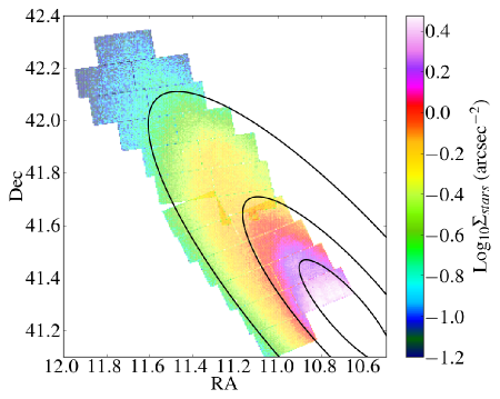
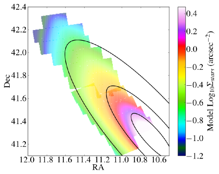
Figure 3.— Mapping the stellar surface density $\Sigma_{stars}$ (Sec. 4.1). (Left) Log₁₀ of the surface density of NIR-detected RGB stars (in arcsec^-2) with $18.5>F160W>21.0$ and $F160W>0.3$, calculated within $15\arcsec$ wide pixels. Outside of the dense inner bulge, the surface density falls smoothly with increasing distance from the center, with no obvious “holes” caused by regions of high dust extinction. For reference, we plot solid ellipses to represent the isophotes expected for an inclined disk with a position angle of 38.5^∘, inclination of 74^∘, and major axis lengths of 0.25^∘, 0.55^∘, and 1.05^∘; compared to these locii, it is clear that the internal stellar density distribution of M31 is complex, showing multiple components. (Right) A smooth model of the NIR surface density, generated from the sum of 12 Gaussian radial surface density profiles, each with a different position angle and inclination. The model reproduces the observed distribution to within $\sim$15% at all radii.

To minimize the effect of incompleteness and magnitude biases, we impose additional magnitude cuts beyond those implicit in the signal-to-noise cut. We use artificial star tests to define the 50% completeness limit, $m_{50}$, in each filter (i.e., the magnitude for which a star has a 50% chance of being detected) for a large number of fields across our survey area. Fainter than the 50% completeness magnitude, the detection fraction falls dramatically while the photometric bias rises, due to an increase in the fractional flux contributed by blends with faint undetected stars. For each filter we fit a polynomial to $m_{50}$ as a function of the local stellar density, as determined by a multicomponent model fit to the log of the stellar surface density in bright RGB stars (i.e., right panel of Figure 3). The data and polynomial fits are shown in Figure 4. We then use the local surface density to define a spatially-variable magnitude cut at $m_{50}$ that we apply to the photometry. The effect of the 50% completeness cut can be seen in Figure 9, which shows $m_{50}$ superimposed on CMDs constructed from low extinction regions at a range of representative local densities. We make the F160W cut even more stringent (by $\Delta m_{50,F160W}=0.5{\rm\,mag}$) than shown in Figure 9 to remove stars near the bottom of the CMD, where even small amounts of reddening would move the star beyond the magnitude limit in F110W; such stars are numerous but do not add significant leverage in measuring the reddening distribution and thus we wish to minimize their impact on the fit to the CMD.

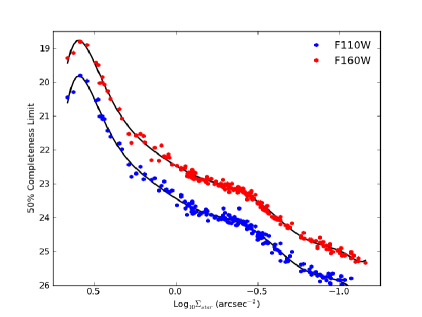
Figure 4.— The depth of the photometry as a function of radius. The blue and red points show the 50% completeness limit $m_{50}$ as a function of log₁₀ of the local stellar surface density in bright RGB stars, for the F110W and F160W filters, respectively. The solid lines show 10th order polynomial fits to the data, used to interpolate to an appropriate limiting magnitude at each position in the galaxy. The PHAT photometry is crowding-limited, and thus the limiting magnitude is a strong function of the local stellar surface density. The apparent roll-off in the inner disk (at high surface densities in the left side of the plot) is an artifact of the extraordinarily high crowding levels in the inner bulge, which lead to biases in the photometry; while we include these regions for completeness here, we do not actually analyze their $A_{V}$ distributions.

In addition to culling poorly measured stars, we also make an initial correction for spatially-dependent variations in the photometry across the WFC3/IR chip. The version of the photometry used in Williams et al. (2014) does not include spatial variation in the PSF model in the NIR. This can lead to systematic variations in the photometry across the face of the camera, such that stars in one position on the chip will be measured systematically brighter or fainter than in another. Errors in the large scale flat-field can also lead to similar issues. While these effects are partially corrected for by DOLPHOT’s perturbations of the PSF model, small differences on the scale of a hundredth of a magnitude persist. Our sensitivity to dust depends on small shifts in the NIR color, and thus failure to correct for these effects will limit the sensitivity we have to low levels of attenuation.

We develop a position-dependent correction map for the color by analyzing fields in the outer galaxy that have low extinction on the Draine et al. (2014) emission-based dust map. We use 54 individual fields in Bricks 2, 6, 8, 10, 11, 12, 14, 18, 19, 20, 22, and 23, and calculate each star’s color relative to the RGB locus. We bin the stars as a function of position on the NIR chip in a 40$\times$40 grid, keeping only bright stars that fall in positions where the extinction $A_{V,emission}$ predicted by Draine et al. (2014) is less than $0.15{\rm\,mag}$, and then calculate the median of the color offset. The resulting map shows coherent structure, with redder colors found for the largest values of $Y$, peaking at the middle of the range in $X$. Bluer colors are found for the lowest values of $Y$, peaking for large values of $X$. The amplitude of the variation is small, with peak-to-peak variations of roughly $\pm 0.01{\rm\,mag}$, comparable to the amplitude seen by Williams et al. (2014, ; see their Fig. 24). The structure appears robust with respect to different choices of magnitude range, binning scheme, mean vs. median, field choice, etc. We find similar patterns when using colors derived from measuring the magnitude of the red clump, although the resulting maps are less accurate due to the red clumps larger intrinsic width.

We apply this correction to all of the photometry before beginning analysis, choosing to modify the F160W magnitude to produce the required color shift. Although the pattern in the map of color shifts undoubtedly reflects differences in photometry between F110W and F160W, we cannot deduce the magnitude shifts from the RGB color alone. In practice, the effect of shifting magnitudes by $\pm 0.01{\rm\,mag}$ is minimal, since these shifts are significantly smaller than the magnitude error of the size of the magnitude bins we use when fitting the observed RGB.

4.2. Generating a Model for the Unreddened RGB

Building a model of the unreddened RGB that includes spatial variations is essential to mapping the extinction. Our extinction mapping technique relies on detecting stars that are “redder than expected”, and thus spatial variations in the expected stellar colors can be misinterpreted as reddening if the underlying RGB model is incorrect. We therefore must build a model for the unreddened RGB and red clump that captures as much of these variations as possible.

Unfortunately, stellar population gradients, density-dependent photometric quality, and projection effects make the CMD structure of the RGB and red clump complex and difficult to model. Generating a theoretical model for the unreddened RGB would require solving for the detailed star formation history across the disk to account for gradients in age and metallicity, while also building a model for projection effects and photometric errors. Such a model would be subject to errors in the disk model, the characterization of photometric errors throughout the disk, and the star formation history itself, as well as any errors in the underlying stellar isochrones and atmospheric models, which can be particularly significant for cool stars in the NIR.

Instead of trying to simulate these effects, we adopt an empirical approach. We isolate low-extinction regions throughout the galaxy, and then bin the stars in these regions to generate a model CMD. We create these models as a function of the local stellar surface density, which captures variations in both the underlying stellar populations and in the photometric errors.

Here we discuss the process used to generate the spatially-dependent model of the unreddened RGB, the properties of the RGB itself, and the associated uncertainties.

4.2.1 Spatial Variations in the NIR RGB

Almost all of the stars in the PHAT NIR photometry lie on the RGB or in the “red clump” found at the red end of the horizontal branch. These stars span a range of ages ($\gtrsim 1{\rm\,Gyr}$) and metallicities, depending on the exact star formation and chemical enrichment history of M31. The colors of these stars depend on their age and metallicity, with older and more metal rich stars favoring redder colors. The RGB’s mean color and width can therefore change as a function of position if the past star formation history and enrichment varies spatially. Metallicity and age gradients are common in disk galaxies, and distinct structures such as M31’s spheroid and bar may likewise have star formation histories that differ from those in the disk. The net result is that the structure of the RGB is likely to vary with position within the galaxy. While the RGB is sufficiently old that dynamical evolution will have smoothed out any sharp features, failure to account for the anticipated smooth variations will lead to errors when trying to model the color distribution of RGB stars.

The spatial variations in RGB and red clump structure can also be subtly altered by viewing angle. The RGB and red clump are dominated by older stars, many of which were born in or dynamically heated into a thicker disk. When this disk is inclined, a range of radii will be present along a given line of sight. The stars at a given projected radius are therefore a blend of the stars from a range of radii and scale heights. The degree of this “projection mixing” will depend on distance from the major axis. Stars on the major axis come from a range of scale heights and azimuthal angles, but will all be at the same radius. Away from the major axis, however, projection effects will mix together stars from a range in radii, not just scale height. This projection mixing will leave a signature on the structure of the RGB and red clump as a function of distance from the major axis, if the age and metallicity vary with radius and if the disk is thick compared to the scale length over which the intrinsic RGB properties vary. We currently do not try to capture the impact of projection mixing, which requires knowledge not just of the radial gradients in the stellar populations, but on the amplitude of such gradients with scale height; we expect that projection mixing will be second-order compared to the radial gradient and photometric errors.

Finally, in addition to spatial variations due to projection effects and in the intrinsic properties of the RGB and red clump, we expect there to be spatial variations in the quality of the photometry. The NIR observations of M31 are highly crowded, which affects the behavior of photometric errors, biases, and depth. In general, all of these quantities are adversely affected when the stellar density increases, such that photometric errors and biases are larger at a given magnitude, and the 50% completeness limit is much brighter (see Williams et al., 2014). We therefore expect the RGB to be broader and shallower in regions of the highest stellar density.

To characterize the unreddend RGB as a function of position, we use the stellar surface density $\Sigma_{stars}$ to track position, rather than projected radii. We choose to work in the space of stellar surface density (rather than radius), because the local surface density is the dominant factor setting the quality and depth of photometry for crowding-limited images. This variation in photometric quality has far more of an effect on the CMD morphology of the unreddened RGB than do the radial gradients in the underlying stellar population (which are small, as we show below). Moreover, the local density is an equally good proxy for “distance from the center of M31”, allowing it to track stellar population gradients without needing to be tied to a specific model for the 3-dimensional stellar distribution; a single disk model is not appropriate where the structure of the galaxy is far more complex (e.g., the inner bulge and bar (e.g., Beaton et al., 2007) and the outer warp (Innanen et al., 1982)). The decrease in the stellar density with radius, and the structurally complex inner region can be seen in Figure 5, where we plot the log of the surface density in bright RGB stars (from Figure 3) as a function of the projected major axis for a fiducial inclined disk model.

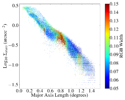
Figure 5.— The mapping between Log₁₀ of the surface density of bright RGB stars and the distance along the major axis (see discussion in Sec. 4.2). Points are color coded by the standard deviation of the upper RGB, relative to a fiducial locus, as in Figure 6. The color coding indicates the position of the major star-forming ring and the more minor outer star-forming arm, at $\sim 0.75{{}^{\circ}}$ and $\sim 1.15{{}^{\circ}}$ from the center, respectively. The outer disk declines approximately as an exponential disk, but the inner disk is multivalued, because the single inclined disk model used to calculate the major axis length is not appropriate for the complex inner disk. The falloff towards the center ($\lesssim\!0.2^{\circ}$) is due solely to increasing incompleteness in the highly crowded inner bulge.

4.2.2 Identifying Candidate Low Extinction Regions

We isolate low-extinction regions by identifying areas where the RGB is narrow and unreddened. We first divide the stars within each PHAT “brick” into bins $15\arcsec$ on a side ($\sim\!57{\rm\,pc}$) and then make a broad cut in color and magnitude to isolate stars on the upper RGB ($19.0\!<\!{\rm F160W}\!<\!22$). These regions are larger than our fiducial $25{\rm\,pc}$ analysis regions to ensure there are enough stars on the upper RGB to provide reliable measurements of the RGB’s width and color. We then calculate mean color of the RGB relative to a fiducial RGB locus (approximated as ${\rm F110W}-{\rm F160W}=a_{0}+a_{1}({\rm F160W}-m_{0})+a_{2}({\rm F160W}-m_{0})^{2}$ where $m_{0}=22.0$, $a_{0}=0.752$, $a_{1}=-0.1$, $a_{2}=-0.006$). We also calculate the standard deviation of the distribution of color differences between RGB stars and the fiducial locus; we refer to this standard deviation as the “width” of the RGB in subsequent plots. This definition of “width” is somewhat sensitive to differences in slope between the fiducial and the actual RGB. It therefore does not solely indicate broadening, given that an RGB with a different slope than the fiducial could also have a significant width by this measure, even if it were intrinsically narrow. However, such slope differences are modest and vary smoothly with radius (Fig. 10; left panel), and thus the “width” will still identify a locally broader RGB.

Figure 6 shows the resulting maps of the width of the RGB and the mean color shift of the stars with respect to the fiducial RGB locus. The main gas-rich star-forming rings clearly show up as regions that have larger RGB widths and redder colors than is typical for their location in the galaxy. The shift in mean color is also largest eastward of the major axis, which is the near side of M31. In this region, a much larger fraction of stars are reddened, as is obvious from optical images of the galaxy.

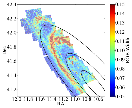
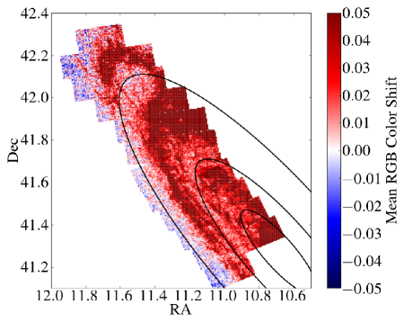
Figure 6.— Maps of the width and color of the upper RGB (Sec. 4.2.2). (Left) Standard deviation of bright ($19.0<F160W<22$) stars around a fiducial RGB locus, as a function of position. The RGB is broader in regions of higher extinction. The typical width of the RGB also increases towards the inner galaxy due to larger photometric errors from stellar crowding and undetected blends, and potentially due to a broader range of intrinsic properties in the underlying stellar population. (Right) The mean color of bright ($19.0<F160W<22$) stars relative to a fiducial RGB locus, as a function of position. The mean colors are redder in regions of high extinction, as expected. There are also radial trends towards bluer relative colors in the inner disk. However, this does not indicate a systematic bluing of the population, and instead reflects increasing mismatch between the RGB and the fiducial locus. Note also that there is some repeating structure in the mean RGB color that mimics the positions of the WFC3/IR fields. This structure is likely to be due to residual $<0.015\,{\rm mag}$ errors in the WFC3/IR flat fields, or in the spatially-varying PSF model. Ellipses are at the same location as in Figures 3.

We isolated the low-extinction regions from these maps as follows. First, we assembled a list of candidate low-extinction regions for each brick. Within each brick, we tagged regions by their projected major axis length for the fiducial inclined disk model, and sorted these subregions into 20 bins of radius within each brick. Then, within each of those radial bins, we identify candidate low $A_{V}$ regions by tagging the 20% of subregions that have the narrowest RGBs, as characterized by the standard deviation in the color of their RGB relative to the fiducial RGB locus. This process guarantees that candidate regions are identified uniformly throughout the brick. We repeat this process for every brick and then merge the candidate low-extinction regions into a list that is guaranteed to sample the entire area covered by the PHAT data.

4.2.3 Producing an RGB Model as a Function of Local Surface Density

After merging the candidate low-extinction regions from all bricks, we analyze the resulting list to find the lowest exinction subregions associated with a given stellar surface density.

From the list of low extinction candidates, we select the regions that have the narrowest RGBs as a function of local surface density, by including any region that falls below the heavy black lines in the left panel of Figure 7 ($\sigma_{RGB}=0.071+0.0125(\log_{10}{\Sigma_{stars}}+0.2)$ and $\sigma_{RGB}=0.071+0.0235(\log_{10}{\Sigma_{stars}}+0.2)$, for the high and low density regions, respectively). We then impose an additional cut on the color of these regions by iteratively fitting a fourth order polynomial to the mean RGB color relative to the RGB fiducial, and selecting the subset of regions with the narrowest RGB that are also no more than 0.5 standard deviations redder or 7 standard deviations bluer than the polynomial fit; the selected color range is indicated with light solid lines in the right panel of Figure 7. The red selection limit culls any potentially reddened regions and the blue selection limit reduces fields with large contamination on the blue side of the RGB from asymptotic giant branch or red core Helium burning (RHeB) stars. Finally, we compare the surviving regions to the dust map recently published by Draine et al. (2014), and reject any regions that fall where the implied extinction is greater than $A_{V}>0.175$. The stars that fall in the remaining regions are then tagged with the local stellar surface density, and then used to generate model unreddened CMDs.

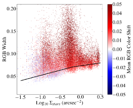
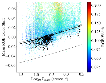
Figure 7.— Identifying low exinction regions using the width and mean color of the RGB, as defined in Sec. 4.2.2. (Left) The standard deviation of the upper RGB, relative to a fiducial RGB locus, as a function of the log of the local stellar surface density of bright RGB stars, color coded by the mean color of the RGB relative to the same fiducial RGB locus. Solid lines show the selection limit below which we identify the lowest extinction regions at each stellar surface density. (Right) The mean color of the RGB relative to the fiducial RGB locus, as a function of the log of the local stellar surface density of bright RGB stars, color-coded by the width of the upper RGB (defined as the standard deviation, relative to the same fiducial RGB locus). Light solid lines indicate the range in color used to exclude regions with possible extinction (upper curve) or high contamination from RHeB and/or AGB stars (lower curve) from the selection region identified in the left panel. Heavy solid points indicate regions that survive both cuts, and which also have low extinction in the Draine et al. (2014) dust map. The location of these points on the disk are shown in Figure 8.

The regions that survive the cuts are highlighted in dark blue in the right panel of Figure 7. There are $\sim 153,000$ stars total in these regions, sampling the full range in local surface density, although not uniformly; for example, there are no low extinction lines of sight identified in the dusty $10{\rm\,kpc}$ star forming ring ($-0.5\lesssim\log_{10}{\Sigma_{stars}}\lesssim-0.2$), and there are many more low extinction regions that sample the diffuse outer disk. The spatial distribution of these regions is shown in Figure 8, superimposed on a map of the width of the upper RGB. By design, these regions lie in the lowest extinction regions of the recently published Draine et al. (2014) dust mass map, derived from models of dust emission. We note, however, that our selection does not ensure that these regions truly have zero extinction. The RGB has a finite width due to photometric uncertainties and stellar population effects, and we cannot detect extinction variations that broaden the RGB by amounts smaller than the intrinsic width.

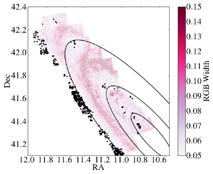
Figure 8.— Location of the lowest extinction regions (blue dots), superimposed on a map of the width of the RGB (e.g., left panel of Figure 6; see Sec. 4.2.2). Ellipses are at the same location as in Figures 3 and 7.

To generate the final model CMD for unreddened stars as a function of local surface density, we group the unreddened stars into bins of $\log_{10}{\Sigma_{stars}}$. We first rank the regions by their local surface density, and then use a sliding, adjustable bin to generate CMDs which each contain at least 2500 bright RGB stars in the range $19\!<\!{\rm F160W}\!<\!21.5$). Each of the resulting set of bins contain comparable numbers of stars, but do not sample equal ranges of local surface density; in the low surface density outer disk, one must merge stars in a wider range of $\log_{10}{\Sigma_{stars}}$ to reach the same total number of stars. We also allow sequential bins to overlap by one third, to provide a smoother interpolation over local density. To avoid having unnecessarily high numbers of nearly identical adjacent bins, we then merge neighboring density bins together until there is a step of at least $\Delta\log_{10}{\Sigma_{stars}}=0.05$ between each bin. We then keep a record of the mean and the range of $\log_{10}{\Sigma_{stars}}$ associated with each bin. When fitting data, we adopt the model CMD from the bin with the closest mean surface density to that of the region being analyzed.

4.2.4 Properties of the RGB in Low Extinction Regions

Four representative CMDs of the low extinction regions, in narrow ranges of local surface density, are shown in Figure 9. These CMDs are extremely clean, showing only a narrow RGB sequence. The CMDs also demonstrate the quality of the photometric cuts, as measured by the nearly total absence of spurious detections near the magnitude limit.

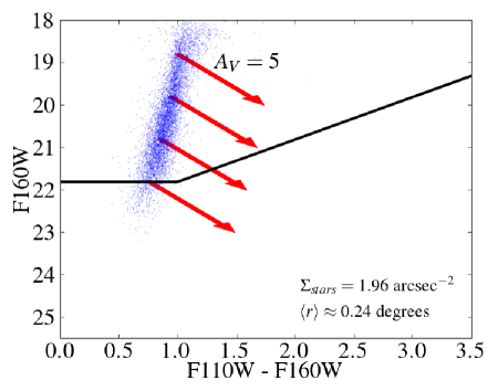
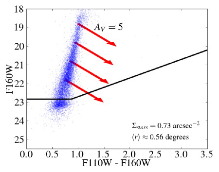
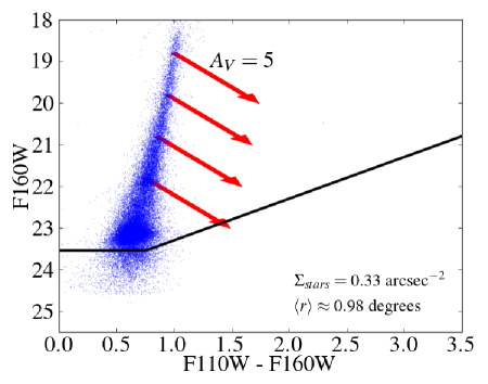
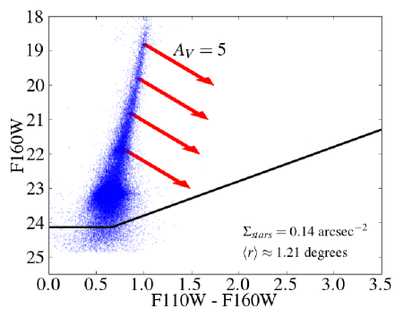
Figure 9.— CMDs of stars in 4 unreddened regions, spanning a range of local RGB surface density $\Sigma_{stars}$ (Sec. 4.1) and/or deprojected semi-major axis distance $\langle r\rangle$ (Sec. 4.2). The black lines indicate the 50% completeness limits adopted at that stellar surface density. Note the near absence of stars redward of the CMD, indicating the quality of the photometric cuts and of the identification of low extinction regions. Red arrows show the expected effect of 5 magnitudes of extinction in $V$. Extinction will cause fainter stars to drop below the completeness limit at lower $A_{V}$ than for brighter stars. The effect of the magnitude cuts on the range of observable $A_{V}$ is more severe in the inner disk, where the cuts are closer to the tip of the RGB. The RGB in this region is also intrinsically wider, making it more difficult to measure small offsets due to reddening.

In Figure 10, we show the properties of the unreddened RGB as a function of magnitude (calculated in bins of $0.15\,{\rm mag}$), in each of the resulting bins of local surface density. The mean color of the RGB (left panel) is systematically bluer and the RGB slope is steeper towards low local surface densities (i.e., towards the outer disk), as would be characteristic of an increasingly metal poor population (see Gregersen et al., 2015). However, the shift in RGB morphology is extremely small between adjacent bins, such that our choice to bin in $\log_{10}{\Sigma_{stars}}$ leaves no detectable imprint on the extinction maps that are eventually derived from the unreddened CMDs.

The right panel of Figure 10 shows the standard deviation of the color of the RGB as a function of magnitude. The RGB becomes increasingly narrow at bright magnitudes and towards the outer disk, as would be expected for decreasing photometric uncertainties, and a narrower mixture of stellar populations. There is also a clear floor at $\sim 0.025\,{\rm mag}$, which is due to a combination of the instrinsic width of the RGB, photometric uncertaintes, and systematic calibration errors in the WFC3/IR chip ($\pm 0.01\,{\rm mag}$). The minimum width corresponds to roughly $0.3$ mag of extinction, setting a threshold below which we are significantly less sensitive to broadening due to reddening. We could potentially improve our sensitivity to low-but-not-zero extinction with improved WFC3/IR calibrations if systematics dominate, but may not be able to if this floor is the intrinsic width of the underlying population.

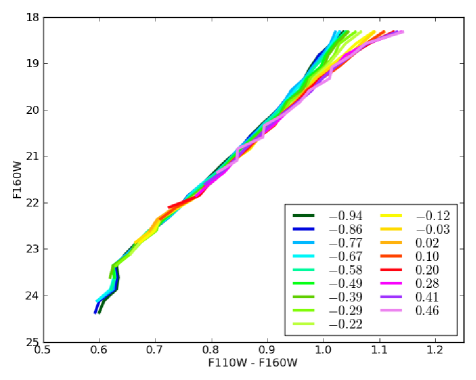
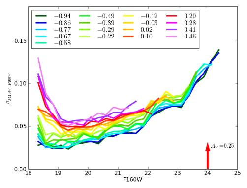
Figure 10.— The morphology and width of the unreddened RGB as a function of position within M31, as characterized by the stellar surface density $\Sigma_{stars}$ . (Left) Color locus of the unreddened RGB as a function of magnitude. Each line corresponds to a bin of $\log_{10}{\Sigma_{stars}}$ (in units of arcsec^-2), which can be mapped to major-axis length using Figure 5). The mean color was calculated in bins of 0.15$\,{\rm mag}$, above the limiting 50% completeness magnitude shown in Figure 4. The morphology of the RGB varies slowly and smoothly from the inner regions (pink) to the outer disk (dark blue). The RGB can be traced to fainter magnitudes in the less crowded outer regions, due to the smaller photometric errors and fainter crowding limit. (Right) Standard deviation of stars around the mean color locus as a function of magnitude, calculated in the same bins as in the left panel. The arrow indicates the expected shift in color for an extinction of $A_{V}=0.25$. See Sec. 4.2.4 for a discussion of this figure.

4.2.5 Limitations in Building an Unreddened RGB

There are a number of unavoidable limitations in our procedure for generating a model of the unreddened distribution. While these effects are quite small in terms of their effect on the structure of the RGB, they can potentially affect the inferred extinctions. In addition to their impact on the model of the unreddened RGB, these effects will also impact measurements of the redding at low extinction. We now discuss each of these in turn.

The Finite Width of the RGB

The width of the RGB (Figure 10) creates a limit on the lowest extinction we can reliably identify at a given location. If the color change produced by a given $A_{V}$ is much smaller than the typical width of the RGB, then small redward shifts of the CMD will not be detectable. The finite width of the NIR RGB thus directly affects our ability to accurately identify the lowest extinction lines of sight.

Although we have taken great pains to identify the lowest reddening regions throughout the galaxy, there is no guarantee that these are truly zero reddening lines of sight, due to the fact that low level of diffuse dust may not produce measurable shifts in the NIR colors and/or width of the RGB. We have attempted to mitigate for this effect by using the Draine et al. (2014) dust emission maps to place more stringent limits on the local extinction than are possible with the NIR CMD alone. However, due to background subtraction, the Draine et al. (2014) maps have uncertainties at low extinction as well, such that some stars with $A_{V}>0$ may still remain in our “zero reddening” model CMD. The resulting model CMD would be biased slightly to the red, and would lead to underestimating $A_{V}$ when modeling the observed CMD.

We can estimate the amount of reddening that could be present in our “unreddened” CMD by inspecting the widths of the RGB at bright magnitudes, shown in the right panel of Figure 10. If the width of the RGB is $\sigma_{F110W-F160W}\lesssim 0.03$ over a reasonably well populated part of the RGB, then one could expect to identify extinction at the level of $A_{V}=0.25$, indicated by the vertical arrow. We therefore expect that the model of the unreddened CMD could be “contaminated” with reddened regions with no more than this level of extinction. Inspection of the RGB widths in Figure 6 suggests that identifying low reddening regions will be harder in the inner galaxy, where the RGB appears to be wider, both due to higher photometric errors from crowding, and from the wider range of metallicities present as one nears M31’s bulge. However, the overall level of extinction in the inner galaxy appears to be low (Draine et al., 2014), which may perhaps mitigate against this effect.

Including bluer filters in our analysis could potentially improve our ability to correctly identify low extinction regions, while also giving more sensitivity in measuring $A_{V}$. In Appendix A we discuss the trade-off between the intrinsic width of the RGB and the sensitivity of RGB color to extinction in other PHAT filter combinations.

Stellar Population Gradients

Spatial variation in M31’s underlying stellar population pose another possible obstacle to creating a realistic model of the unreddened CMD. We construct models from stars in individual low reddening regions, but frequently, these are far from the individual pixel being analyzed. Thus, if there are spatial variations in the stellar population, we may sometimes use a model CMD that does not correctly reflect the local population. To first order, this should not present a severe problem because we match the local stellar density of the model to the pixel being analyzed, which isolates regions at comparable deprojected radii, and thus of similar underlying stellar population. Empirically, Figure 10 shows that the RGB color and width is a very weak function of local stellar density, particularly where $\log_{10}\Sigma_{stars}<-0.2{\rm\,arcsec^{-2}}$. Thus, systematic offsets in the structure of the RGB are likely to involve color differences of only a few hundredths of a magnitude, which would produce a very small bias in the modeled RGB. The only place where we anticipate that stellar population gradients might significantly affect the model unreddened CMD is in the inner regions of the galaxy where the stellar populations change more rapidly with radius, and where the structure of the galaxy is complex (due to M31’s bar, and multi-component bulge; see Figure 5 and Gregersen et al. (2015)).

A potentially more significant impact of stellar population gradients comes through their effects when viewing an inclined disk (as in M31). Projection effects lead to pixels along the minor axis having stars from a wider range of radii than along the major axis. The net result is that while matching of the stellar densities correctly matches the photometric properties of the RGB, it may not successfully match the underlying color and shape of the RGB, due to a mismatch in the stellar populations between the model and the pixel being analyzed.

Foreground Extinction from the Milky Way

The final limitation when constructing a model for the unreddened CMD is that there may be foreground dust extinction from the Milky Way or from a diffuse dust halo in M31 itself. This foreground would not affect our results if it were uniform, because our measurement is fundamentally relative; if both the reddened and “unreddened” stars are affected equally, the measurement of the reddening relative to the unreddened model is still sound even if the “unreddened” model has been affected by dust in the Milky Way foreground. If the foreground dust is not uniform (which indeed is most likely), then it broadens the RGB in the model for the unreddened CMD, due to including lines of sight with different reddenings. The net result will be to reduce sensitivity to low levels of reddening within M31. Unfortunately, one cannot use maps of the Milky Way dust (e.g., Schlegel et al., 1998; Schlafly & Finkbeiner, 2011) to correct for the foreground dust, since these maps fail when there is a bright background source of FIR emission (such as M31) that dominates the emission from the Milky Way.

While the list above describes the principal limitations in constructing the unreddened CMD, there are additional uncertainties associated with the model fitting itself. We discuss these below in Sec. 5.3.2, and make empirical tests of systematics in our final maps in Sec. 6.4.

4.3. Generating the Model Reddened CMD

Our data is set of F160W magnitudes $m_{i}$ and F110W$-$F160W colors $c_{i}$. We therefore need to translate our adopted model for the expected distribution of extinctions $p_{A}$ and/or reddenings $p_{\mathcal{E}}$ into a model of the expected color magnitude diagram for a given set of model parameters $\vec{\theta}=\{\widetilde{A_{V}},\sigma,f_{red},\delta_{c}\}$, given the empirical model for the distributions of colors and magnitudes of unreddened RGB stars that we derived in Sec. 4.2.3. In other words, we wish to derive $p_{CMD}(c,m|\vec{\theta})$, the probability of finding a star at color $c$ and magnitude $m$, given $\vec{\theta}$. This model will depend on the local surface density $\Sigma_{stars}$, but we do not make this surface density dependence explicit, for notational compactness.

Before proceding with the calculation of $p_{CMD}$, we take two steps to increase the computational efficiency. First, we bin both the data and the models into bins of color and magnitude. We use a grid spacing of 0.015$\,{\rm mag}$ in color and 0.2$\,{\rm mag}$ in magnitude. This choice guarantees that there are at least 2 pixels across the 1$\sigma$ width of the narrowest RGB, effectively Nyquist sampling the width. Experiments with smaller bins produced no noticeable changes in the resulting extinction maps, while dramatically increasing the computation time.

Second, we translate all F160W magnitudes into “reddening-free” magnitudes $q$, defined as

$$\begin{split}q\equiv{\rm F160W}-(({\rm F110W}-{\rm F160W})-c_{0})\\ \times\frac{A_{F160W}/A_{V}}{(A_{F110W}/A_{V})-(A_{F160W}/A_{V})}\end{split}$$ (9)

where $c_{0}$ is an arbitrary color for which $q\equiv{\rm F160W}$. With this transformation, increases in extinction will cause a star’s color to redden, while leaving the reddening-free magnitude unchanged. With this skewed version of the CMD, changes in the extinction move stars horizontally in the grid, rather than diagonally (i.e., the reddening vector becomes horizontal). We can then do 1-dimensional convolutions when calculating the reddened CMD, rather than more computationally expensive 2-dimensional convolutions. We will therefore calculate $p_{CMD}(c,q|\vec{\theta})$ rather than $p_{CMD}(c,m|\vec{\theta})$.

The next step in generating $p_{CMD}$ is to define what region of the CMD will be fit. We restrict our analysis to regions occupied by RGB stars by generating a mask. The blue boundary of the mask is defined to be 2.5$\sigma$ blueward of the RGB (Fig. 10) to reduce contributions from AGB and RHeB stars. The upper boundary is fixed at $q=18.5$, which is approximately the tip of the RGB. The lower faint boundary and the right diagonal boundaries were set by the adopted F160W magnitude limit ($m_{50,F160W}-0.5$) and the 50% completeness limit in F110W, respectively, both translated into the reddening-free CMD. All normalizations and comparisons with data are restricted to be within the unmasked regions.

Within each bin of local stellar surface density, we grid the unreddened stars into a CMD where the reddening-free magnitude $q$ has replaced F160W, eliminating stars that fall in the masked region. We then normalize the binned CMD so that it integrate to one over the unmasked area. We refer to the final binned, masked, normalized probability distribution for unreddened stars as $p_{unreddened}(c,q)$.

We then generated the probability distribution for the reddened stars, $p_{reddened}(c,q|\widetilde{A_{V}},\sigma)$, by convolving the binned unreddened CMD with a 1-dimensional log-normal kernel, where the properties of the kernel are set by $\widetilde{A_{V}}$ and $\sigma$. We then added the reddened and unreddened model CMDs together to generate the model for the combined CMD $p_{unreddened+reddened}(c,q|\vec{\theta})$ after weighting them by appropriate fraction of reddened stars:

$$\begin{split}p_{unreddened+reddened}(c,q|\vec{\theta})=(1-f_{red})\,p_{unreddened}(c,q)\\ +f_{red}\,p_{reddened}(c,q|\widetilde{A_{V}},\sigma).\end{split}$$ (10)

We then reapply the mask to $p_{unreddened+reddened}$ and renormalize.

We also include a third component to model the noise from potentially bad photometry. Occasionally, spurious sources will be detected with colors and magnitudes consistent with being reddened RGB stars. These sources are rare, but not impossible, and thus we need to include an additional component in our model that allows there to be a small chance of an individual source being spurious, rather than requiring every star redward of the RGB to be due to dust reddening. To model the CMD contribution from noise, $p_{noise}$, we identify stars that are more than 3.5$\sigma$ redward of the mean RGB color in regions that were identified as being “unreddened”. These red stars are unlikely to be due to intervening dust, and instead are due to occasional photometric errors when doing crowded field photometry. These anomalous red stars are then gridded into a “noise CMD”, $p_{noise}(c,q)$, and then re-added into the sum of the unreddened$+$reddened models in the proportion with which they were found in the original unreddened CMD. Letting $f_{noise}$ be the fraction of stars in the catalog of unreddened stars were classified as noise,

$$\begin{split}p_{CMD}(c,q|\vec{\theta})=(1-f_{noise})\,p_{unreddened+reddened}(c,q|\vec{\theta})\\ +f_{noise}\,p_{noise}(c,q)\end{split}$$ (11)

The fraction of pixels in the noise model was never more than 1.5% in any bin of local stellar surface density, and was less than 0.5% in 3/4 of the bins.

Finally, we introduce a fourth parameter $\delta_{c}$ that allows the color of the unreddened CMD to shift by a few hundredths of a magnitude, with the goal of absorbing any residual issues with the spatially-dependent WFC3/IR calibration/photometry correction discussed in Sec. 4.1. Because the photometric correction we applied in Sec. 4.1 was calculated on a coarse grid of chip position, it does not accurately trace rapid changes with position, particularly those near the edges of the chip; these residual issues can be seen as slight bands in Figure 6 that trace the edges of the NIR chip in adjacent observations. In addition, a handful of fields show small global shifts in RGB color, most likely due to a small error in the aperture correction that was applied to the entire field. Both of these residual systematic photometry errors translate directly into features on the resulting extinction map if not corrected for.

An example of an unreddened and reddened CMD are shown in Figure 11.

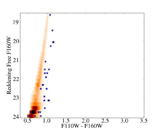
Figure 11.— Comparing a binned unreddened CMD (left) to a reddened model including noise (right). Star symbols show the location of stars found in a $25{\rm\,pc}$ pixel in Brick 15. The best fit parameters for that pixel are used in the reddened model. Note that the vertical axis is not F160W magnitude, but instead is the “reddening-free” F160W magnitude $q$ (eqn. 9), such that changes in the amount of extinction/reddening moves stars horizontally.

4.4. Fitting the Reddened CMD

The model CMD shown in Figure 11 has three adjustable parameters — the median $\widetilde{A_{V}}$ of the log-normal distribution of extinctions, the dimensionless width $\sigma$ of the same distribution, and the fraction of reddened stars $f_{red}$ (eqns. 1 & 2) – in addition to one parameter $\delta_{c}$ to help absorb any residual issues in spatially variable photometry. We solve for these parameters and their uncertainties within small spatial regions of the PHAT imaging data, using MCMC fitting to find the most probable fit and the associated uncertainties, subject to sensible prior probability distributions (“priors”) on the values of the parameters. The choice of priors is discussed in Sec. 4.4.1 below.

Specifically, we use $p_{CMD}(c,q|\vec{\theta})$ derived in the previous section to calculate the probability of finding a star at color $c$ and reddening-free magnitude $q$, for a given set of parameters $\vec{\theta}=\{\widetilde{A_{V}},\sigma,f_{red},\delta_{c}\}$, assuming a model for an unreddened CMD at the local surface density $\Sigma_{stars}$.

The total probability distribution function $p_{total}$ of measuring a set of $N$ independent and identically drawn observations $\{c_{i},q_{i}\}$ is then

$$p_{data}(\{c_{i},q_{i}\}|\vec{\theta})=\prod_{i=0}^{N}p_{CMD}(c_{i},q_{i}|\vec{\theta}).$$ (12)

We do not concern ourselves with the variation in the number of stars per CMD point, given that any variations due to the loss of highly extincted stars is expected to be extremely small, adding little useful information to the fit.

We are interested not in the probability distribution function (PDF) of a given set of observations given the parameters of the adopted reddening model, but instead are interested in the posterior probability distribution function for the reddening parameters $\vec{\theta}$, given the set of observations $\{c_{i},q_{i}\}$. We therefore use Bayes theorem to derive

$$p_{param}(\vec{\theta}|\{c_{i},q_{i}\}) \propto p_{data}(\{c_{i},q_{i}\}|\vec{\theta})\,p_{prior}(\vec{\theta})$$ (13)

$$\propto \prod_{i=0}^{N}p_{CMD}(c_{i},q_{i}|\vec{\theta})\,p_{prior}(\vec{\theta}),$$ (14)

where $p_{prior}(\vec{\theta})$ encodes any prior information on the values of the parameters.

4.4.1 Choice of Prior Probability Distributions

We chose specific forms for $p_{prior}$ to limit the parameters $\vec{\theta}$ to physically plausible values. We chose the prior in $\widetilde{A_{V}}$ to require that the extinction be greater to or equal to zero. For $\sigma$, we adopt a wide log-normal distribution where the most probable value of $\sigma$ is 0.3, which is characteristic of extinction distributions seen in the Milky Way (e.g., Kainulainen et al., 2009), and the dimensionless log-normal width of the prior on $\sigma$ is 0.3. This choice also restricts the value of $\sigma$ to be greater than zero. We adopt a narrow, flat-topped prior for $\delta_{c}$, since we expect the photometric systematics to be small (i.e., as the same order as the large scale systematics corrected for in Sec. 4.1), but do not have a strong prior on the exact value. We adopt a functional form similar to a gaussian with $\sigma_{\delta}=0.035$, but with the exponent raised to the fourth power, rather than squared; this change produces a peaked distribution with a flatter top and faster fall-off than a gaussian.

When setting the prior for $f_{red}$, we take a more sophisticated approach than for $\widetilde{A_{V}}$ and $\sigma$. The value of $f_{red}$ is naturally bounded by zero and one, but rather than having a hard limit at each of these values, we instead adopt a prior that increasingly penalizes values of $f_{red}$ that approach these limits. We do so by “regularizing” $f_{red}$ by switching to a closely related parameter that more easily penalizes the reddening fraction becoming zero or 1, while maximizing the prior probability at an arbitrary mean value of $\langle f_{red}\rangle$. Specifically, we adopt a new parameter $x$ such that

$$f_{red}=\left(\frac{e^{x}}{1+e^{x}}\right)^{(\ln{\langle f_{red}\rangle})/(\ln{0.5})}$$ (15)

With this change of variables, $f_{red}=\langle f_{red}\rangle$ when $x=0$, and $f_{red}$ goes to zero or 1 only when $x\rightarrow\pm\infty$. We then adopt a prior that has a mean $\langle x\rangle=0$ and that declines to both positive and negative $x$, which maximizes the prior probability on $f_{red}$ to have the proper mean, while increasingly (but smoothly) penalizing values of $f_{red}$ that approach the extremes of its permitted values.

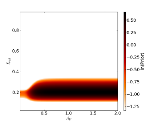
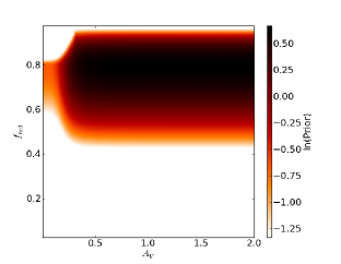
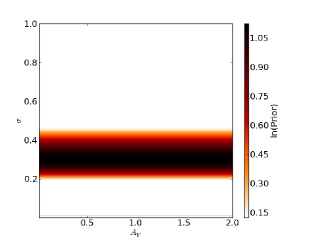
Figure 12.— The log of the priors in $f_{red}$ as a function of $\widetilde{A_{V}}$, for an assumed mean reddening fraction of $\langle f_{red}\rangle=0.2$ (left) and $\langle f_{red}\rangle=0.8$ (center). The right hand plot shows the log-normal prior in $\sigma$, for which the width of the reddening distribution is assumed to be independent of extinction. These priors can be compared to the distribution of recovered values shown in the upper two panels of Figures 16 and 17.

Eqn. 15 requires chosing a value for the expected mean value of $f_{red}$. Naively one might expect $\langle f_{red}\rangle=0.5$, but this is generically only true along the major axis of an inclined disk. For a thickened stellar disk, projection effects lead the stars on the near side of the disk to come from slightly different radii than the stars on the far side of the disk. The number of stars declines approximately exponentially with radius, and thus the fraction of reddened stars at some projected radius can be much higher or lower than 0.5, depending on whether the stars in front of the dust layer are coming from inside or outside the nominal projected radius. As a result, for a moderately thick inclined stellar disk like M31, the fraction of reddened stars should vary significantly from the near side to the far side, by an amount that depends on the inclination and on the thickness of the stellar disk relative to the disk’s exponential scale length. As such, the appropriate value of $\langle f_{red}\rangle$ should vary with position to avoid biasing the derived parameters.

To create a prior that looks as much as possible like the actual data, we developed a simple geometric model for the reddening fraction of a thick, inclined disk. We adjust the properties of this model iteratively, using the observed spatial distribution of $f_{red}$ in regions where the measurement of $f_{red}$ has small reported errors, and thus is essentially unaffected by the prior. Between iterations, the only significant change in the maps of $f_{red}$ are in regions of very low extinction where $f_{red}$ is largely unconstrained by the data, and instead gravitates to the value of $\langle f_{red}\rangle$ set by the prior. The fit converged after only 2 iterations (verifying our assumption that the measured values of $f_{red}$ in low uncertainty regions were unaffected by the choice of prior). The resulting model for $\langle f_{red}\rangle$ has a position angle of $37^{\circ}$, inclination of $78^{\circ}$, and a ratio of vertical to horizontal exponential scale heights of $h_{z}/h_{r}=0.15$. The residuals from this simple model are approximately $\Delta f_{red}=\pm 0.1$.

After setting the most probable value of $f_{red}$ as a function of position and extinction, we set the width of the prior probability distribution by using an asymmetric split normal distribution in $x$. We keep the priors broad, to avoid biases in regions where the simple geometric model for $f_{red}$ is not ideal, and to account for our more uncertain knowledge of the filling factor of molecular clouds $f_{fill}\equiv\mathcal{A}_{cloud}/\mathcal{A}_{pixel}$, where $\mathcal{A}_{cloud}$ and $\mathcal{A}_{pixel}$ are the areas of the gas cloud and the analysis pixel, respectively. We narrow the prior for low extinctions ($\widetilde{A_{V}}<0.3$), where the RGB is only slightly broadened, rather than split into distinct peaks, since these regions will not have sufficient information to constrain $f_{red}$ reliably without the prior. Examples of the resulting priors for regions with $\langle f_{red}\rangle=0.2$ and 0.8 are shown in Fig. 12.

4.4.2 Fitting Parameters in a Pixelized Map

Using these priors and the likelihood (eqn. 12), we use a MCMC sampler to characterize the posterior probability distribution for $\vec{\theta}$ (eqn. 13). We use emcee (Foreman-Mackey et al., 2013), which implements an affine-invariant ensemble sampler to efficiently sample the distribution using a set of coupled MCMC chains (“walkers”; Goodman & Weare, 2010).

We run the MCMC sampler within pixels defined by a dense spatial grid covering the survey area. Our fiducial grid uses square $6.645\arcsec$ pixels, which correspond to $25{\rm\,pc}$ at the distance of M31 ($776{\rm\,kpc}$). M31 is highly inclined, and thus projection effects may make the effective spatial resolution of the survey significantly worse than $25{\rm\,pc}$ in the direction paralleling the minor axis. However, although this degredation in resolution is generically true for disk structures, there is no strong evidence in the Milky Way that molecular clouds are flattened in the same sense as the global galactic disk, rather than being 3-dimensional objects with no preferred direction to their structure. In this latter case, projection does not actually affect the physical resolution; as an extreme example, if molecular clouds were spherical, they would appear to have the exact same size when viewed at any angle. We therefore adopt $25{\rm\,pc}$ as the effective resolution of the dust map, in spite of the inclination of M31’s disk, but recognize that the exact physical resolution could be worse in the direction perpendicular to the major axis.

The adopted $25{\rm\,pc}$ grid size balances the accuracy in $\vec{\theta}$ (which decreases when there are few stars per pixel, as discussed below in Sec. 5.3) and the spatial resolution of the resulting map. We have found that we can produce reliable maps at significantly higher resolution, but only in regions where a large fraction of the stars are reddened.

We oversample the $25{\rm\,pc}$ grid by rerunning the fitting procedure at 4 dithered locations, shifted by 0.5 pixel. We then interleave the resulting 4 dithered maps, producing pixels of $12.5{\rm\,pc}$ on a side. This sub-sampling is roughly analogous to Nyquist sampling a map with $25{\rm\,pc}$ resolution. Each of the interleaved pixels shares 50% of the stars with the adjacent pixels with which it shares a border, and 25% of the stars with the pixels with which it shares a corner. Thus, pixels are not independent of their immediate neighbors, but are completely independent of all other pixels.

Within each $25{\rm\,pc}$ spatial pixel, we use 50 sets of coupled MCMC chains, and take 150 steps to localize the chains near the parameter values that maximize the posterior probability. We then run the sampler for a final 15 steps (i.e., $50\times 15$ samples) to sample the posterior distribution. To deal with memory limitations and allow parallelization, we analyze the pixels in batches, defined by the area of individual survey bricks; when a pixel overlaps adjacent bricks, we use the results for the pixel that contained the largest number of stars. Running the samper for all 22 bricks at all 4 dither positions takes over a week when running on 50 cores.

A representative example of the resulting distribution is shown in Figure 13, for the same model shown in Figure 11. The distribution is smooth and unimodal, as has been the case for all distributions that we have inspected individually. Because of the simplicity of these distributions, we do not save the full probability distribution at each grid point, but instead record the values of the parameters that maximize the posterior probability. We also marginalize the distributions for each parameter, and record the values corresponding to 16%, 50%, and 84% of the parameter distribution (i.e., the median and the $\pm 1\sigma$ points for a Gaussian distribution). When quoting a single value for the uncertainty in each parameter (rather than a range), we define the uncertainty in the $i$-th parameter to be $\Delta\theta_{i}=(\theta_{i,84}-\theta_{i,16})/2$.

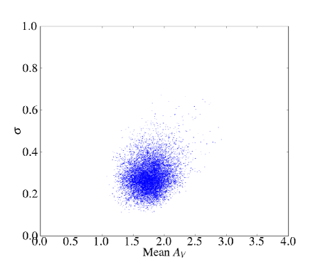
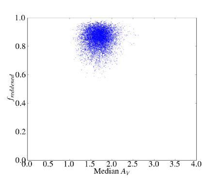
Figure 13.— Samples of the posterior probability distribution function for the width of the log-normal distribution $\sigma$ (left) and the reddening fraction $f_{red}$ (right) as a function of the mean $A_{V}$ (left) and the median $A_{V}$ (right). Samples were drawn for the same $25{\rm\,pc}$ pixel used in Figure 11. Bestfit values and the 16%-84% range are $f_{red}=0.84_{-0.07}^{+0.05}$, $\langle A_{V}\rangle=1.80_{-0.24}^{+0.17}$, and $\sigma=0.24_{-0.06}^{+0.07}$.

We also record the equivalent percentile points for quantities that we derive from the best-fit parameters during subsequent analysis. For example, the mean $A_{V}$ depends on both $\widetilde{A_{V}}$ and $\sigma$ (eqn. 6), so we calculate the marginalized distribution of $\langle A_{V}\rangle=\widetilde{A_{V}}\exp{(\sigma^{2}/2)}$ and record the resulting 16%, 50%, and 84% percentile values, rather than relying on formulas that assume propagation of Gaussian errors in $\widetilde{A_{V}}$ and $\sigma$. The same deterministic translation of uncertainties is used when converting from the regularized variable $x$ back to the reddening fraction $f_{red}$ (eqn. 15).

5. Properties of the Reddening Parameters

Before presenting final maps, we use the results of fitting individual PHAT bricks to demonstrate the overall accuracy of the method. We show results for two independent regions, and discuss the model parameters’ spatial distribution (Sec. 5.1), correlations (Sec. 5.2), and uncertainties (Sec. 5.3). We then discuss the method’s overall susceptibility to systematic errors (Sec. 5.3.2), a point we return to when comparing to other dust tracers in Sec. 6.4 below.

5.1. The Spatial Distribution of Derived Reddening Parameters

The left panels of Figures 14 and 15 show the spatial distribution of $\widetilde{A_{V}}$, $\sigma$, and $f_{red}$ for two of the PHAT bricks that sample regions with different star formation intensities (Bricks 16 and 15, the latter of which contains some of the most intense star formation in the PHAT survey area). Each brick covers an area of roughly $1.5{\rm\,kpc}\times 3{\rm\,kpc}$; see Dalcanton et al. (2012) for details.

Although the reddening parameters are derived independently for each spatial pixel, there are clear coherent features in all the derived parameters across the area, on scales larger than the one pixel coherence expected solely from oversampling the $25{\rm\,pc}$ pixel grid. The distribution of dust extinction shows clear filamentary structure throughout the kiloparsec-scale regions, and is reminiscent of large scale maps within the Milky Way (e.g., Schlegel et al., 1998; Froebrich et al., 2007; Kohyama et al., 2013; Lombardi et al., 2011; Schlafly & Finkbeiner, 2011; Nidever et al., 2012). There is also obvious large scale coherence in the spatial distribution of the reddening fraction $f_{red}$. The width of the reddening distribution $\sigma$ also is spatially coherent and follows the structure in the reddening distribution, but with a much smaller dynamic range.

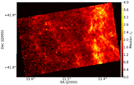
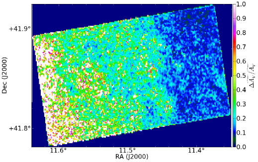
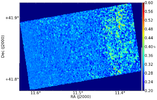
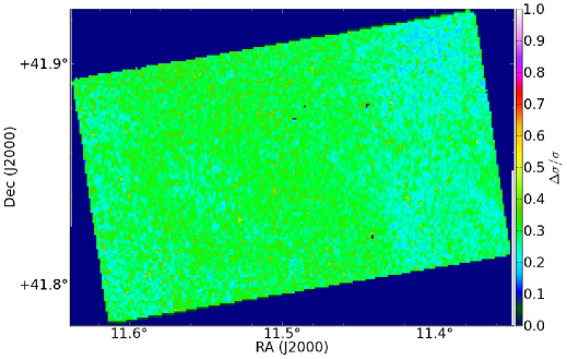
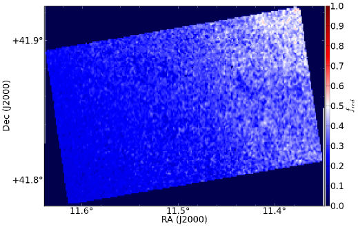
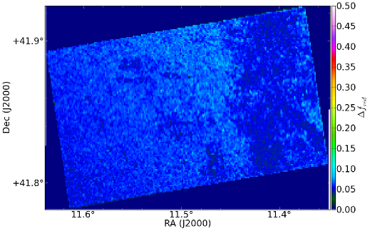
Figure 14.— Left: Maps of the median extinction $\widetilde{A_{V}}$ (top), log-normal width $\sigma$ (middle), and reddened fraction $f_{red}$ (bottom) for Brick 16. In regions of low extinction, the values of $f_{red}$ and $\sigma$ are driven to the most likely value in their priors ($=0.4$). Right: Maps of the fractional uncertainty in extinction $\Delta\widetilde{A_{V}}/\widetilde{A_{V}}$ (top) and the log-normal width $\Delta\sigma/\sigma$ (middle), and the absolute uncertainty in the reddening fraction $\Delta f_{red}$ (bottom). Uncertainties are smallest in the regions of highest extinction. In general, the fractional errors in $\widetilde{A_{V}}$ are much smaller than in $\sigma$.

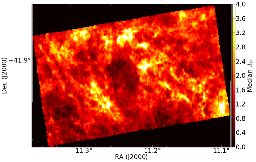
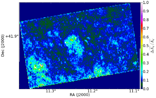
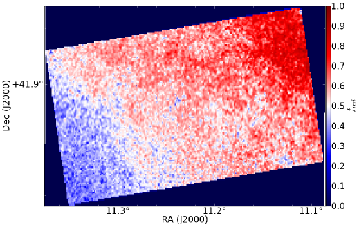
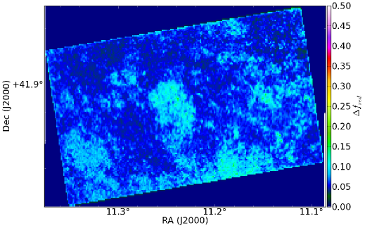
Figure 15.— Same as Figure 14, but for Brick 15, which falls on the $10{\rm\,kpc}$ star-forming ring on the major axis, and thus samples the highest star formation of any of the PHAT bricks. Left: Maps of the median extinction $\widetilde{A_{V}}$ (top), log-normal width $\sigma$ (middle), and reddened fraction $f_{red}$ (bottom). Right: Maps of the fractional uncertainty in extinction $\Delta\widetilde{A_{V}}/\widetilde{A_{V}}$ (top) and the log-normal width $\Delta\sigma/\sigma$ (middle), and the absolute uncertainty in the reddening fraction $\Delta f_{red}$ (bottom). Given that uncertainties are smallest in the regions of highest extinction, Brick 15 has low uncertainties overall.

5.2. Correlations Among the Reddening Parameters

Figures 16 and 17 plot correlations among the different reddening parameters, for the maps in Figures 14 and 15, respectively.

The plots of $f_{red}$ as a function of $\widetilde{A_{V}}$ (upper left) reveal a number of features that are due to either the dust distribution or to the fitting process, or both. First, at high extinction ($\widetilde{A_{V}}\gtrsim 1{\rm\,mag}$), the mean value of $f_{red}$ shows no obvious trend with increasing extinction; this behavior is most noticeable in Figure 17, where the extinction and $f_{red}$ are highest. The simplest interpretation of this behavior is that dusty gas largely fills the entire $25{\rm\,pc}$ pixel when the extinction is high, such that the value of $f_{red}$ reflects only geometrical effects (i.e., the relative position of the stars and the gas along the line of sight). In this high extinction regime, the scatter in $f_{red}$ is due both to the uncertainty in measuring $f_{red}$ (Sec. 5.3 below) and to the intrinsic variation in the relative position of the gas with respect to the stars.

At lower extinctions ($0.3\lesssim\widetilde{A_{V}}\lesssim 1{\rm\,mag}$), the typical value of $f_{red}$ tends to fall with decreasing extinction (albeit with large scatter, particularly in Brick 15, where the value of $f_{red}$ varies significantly across the brick). It is unlikely that the relative placement of gas and stars along the line of sight would “know” about the overall extinction of the gas. Instead, this fall-off may reflect that dusty gas has an increasingly smaller filling factor as the median extinction decreases (see, for example, Figure 2). In this regime $f_{red}$ equals the product of the “geometric” value of $f_{red,geom}$ that one would measure if the gas filled the entire pixel and of the filling factor $f_{fill}$. Thus, if the area covered by gas is smaller for lower extinctions, then one expects exactly the fall-off we observe. Note that in this range of $\widetilde{A_{V}}$ we have not built the decreasing filling factor into the prior (see Figure 12), and thus the decrease effectively reflects the properties of the gas itself. On the other hand, some of the reduced scatter may be due to the increasing role that the prior plays as the information content of the data decreases. At lower extinctions, reddening does not cleanly separate the reddened and unreddened RGB, making measurements of $f_{red}$ more challenging, which increases the weight given to the prior and pulls the measured value of $f_{red}$ closer to $\langle f_{red}\rangle$.

At the lowest extinctions ($\widetilde{A_{V}}\lesssim 0.3{\rm\,mag}$), the relationship between $f_{red}$ as a function of $\widetilde{A_{V}}$ changes again. In this regime, the width of the NIR RGB is comparable to or less than the broadening expected due to reddening. As such, the observed CMD is barely changed by the dust, and the constraints on the reddening parameters becomes extremely weak. As such, the most probable value of $f_{red}$ is driven almost entirely by its prior. In other words, when the posterior probability distribution is very broad, the peak is set primarily by the prior probability distribution function, which in this case drives $f_{red}$ towards $\langle f_{red}\rangle$ as the extinction decreases below $\widetilde{A_{V}}\lesssim 0.3{\rm\,mag}$.

Unlike the clear trends between $\widetilde{A_{V}}$ and $f_{red}$, any trends of $\sigma$ with the other reddening parameters are far weaker. Below $\widetilde{A_{V}}\lesssim 0.75{\rm\,mag}$, the distribution of $\sigma$ is clearly dominated by the prior. Large values of $\sigma$ are only found at higher extinctions ($\widetilde{A_{V}}\gtrsim 1{\rm\,mag}$, most prevalent in Figure 17). Visual inspection of Figures 14 and 15 confirms that larger values of $\sigma$ are associated with regions of high reddening, but Figures 16 and 17 suggest this is largely the effect of the fits being able to move away from the prior when the signal from reddening is strongest. However, while the distribution of $\sigma$ broadens in high extinction regions, it is clearly much more likely to scatter to higher values than lower ones, suggesting that the distribution of reddenings can become much broader, but rarely becomes narrower, as seen by the floor at $\sigma\approx 0.25$. These high extinction regions with broader reddening distributions may reflect differences in the underlying turbulent structure, a breakdown in the log-normal assumption for the reddening distribution, or an increased likelihood of multiple gas layers falling in a single analysis pixel when the column density is high.

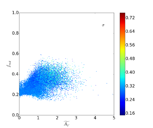
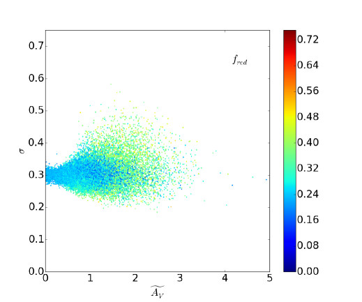
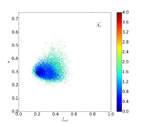
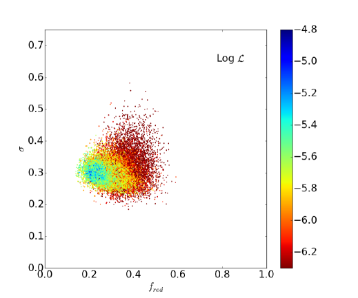
Figure 16.— Joint distributions of derived parameters ($\widetilde{A_{V}}$ vs $f_{red}$, $\widetilde{A_{V}}$ vs $\sigma$, and $f_{red}$ vs $\sigma$, clockwise from top left) for each pixel in Brick 16, color-coded by the parameter labeling the figure; L is the likelihood calculated for the fit. At low $\widetilde{A_{V}}$ ($\lesssim 0.5$), the values of $f_{red}$ and $\sigma$ are clearly pulled towards the maximum probability of the assigned priors ($=0.4$). The bottom right shows $f_{red}$ vs $\sigma$ again, but now color-coded by the log likelihood of the model fit.

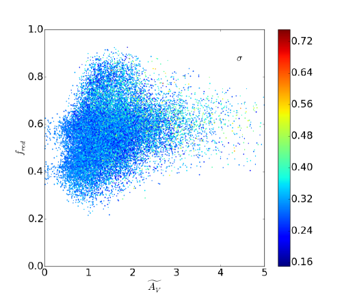
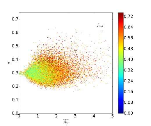
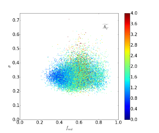
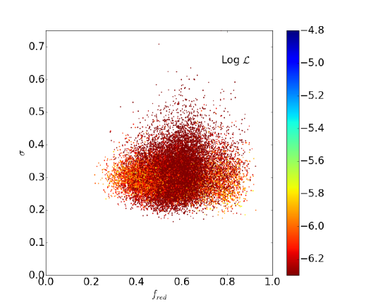
Figure 17.— Same as Figure 16, but for the high star-formation region covered by Brick 15. Joint distributions of derived parameters ($\widetilde{A_{V}}$ vs $f_{red}$, $\widetilde{A_{V}}$ vs $\sigma$, and $f_{red}$ vs $\sigma$, clockwise from top left) for each pixel in Brick 15, color-coded by the unplotted parameter (denoted by the legend). The bottom right shows $f_{red}$ vs $\sigma$ again, but now color-coded by the log likelihood of the model fit.

5.3. Uncertainties in the Reddening Parameters

In the right panels of Figures 14 and 15, we plot the spatial distribution of the uncertainties in $\widetilde{A_{V}}$, $\sigma$, and $f_{red}$ (i.e. $\Delta\theta=(\theta_{84}-\theta_{16})/2$). The uncertainties are clearly not spatially uniform, and instead mimic structures seen in the distribution of $\widetilde{A_{V}}$ and $f_{red}$. This correspondence reflects the fact that the accuracy of the derived parameters depends on how cleanly the extincted stars separate from the unreddened RGB. Thus, the uncertainties are lowest when the median extinction $\widetilde{A_{V}}$ is high (as in Brick 15; Figure 15).

The accuracy of the measured parameters also depends on the number of reddened stars in the pixel. In Brick 15 (Figure 15), the uncertainties on the extinction are low in the upper right corner, where the fraction of reddened stars $f_{red}$ is highest, in spite of the fact that the extinction is not particularly high in that region. Brick 16 (Figure 14) shows a similar gradient in accuracy, but at essentially constant $f_{red}$; here, the fall off in accuracy is due to the lower number of stars per pixel overall, since the stellar density falls significantly from right to left (not shown). Uncertainties are also high for edge pixels, which may not be fully covered by the data. These pixels disappear when we merge the bricks into a contiguous map, because the edges of the bricks overlap significantly. In cases of overlaps, we adopt the fits from whichever overlapping pixel had measurements with the smallest uncertainties.

Because the accuracy depends most strongly on the extinction of the reddened component, in Figures 18 and 19 we plot the fractional uncertainties of $\Delta\widetilde{A_{V}}/\widetilde{A_{V}}$ and $\Delta\sigma/\sigma$, and the absolute uncertainty $\Delta f_{red}$ as a function of $\widetilde{A_{V}}$, for all pixels in Bricks 16 and 15 (whose parameter distributions were shown in Figures 16 and 17).

As expected, there is a clear trend towards better precision at higher extinctions. For large $\widetilde{A_{V}}$, the reddened distribution of RGB stars becomes completely distinct from the unreddened RGB in the CMD, and the distribution typically becomes broader, leading to stronger constraints on the reddening distribution. At high extinctions, the typical uncertainties are smaller than 20% in $\widetilde{A_{V}}$, and smaller than $\pm 0.1$ in $f_{red}$. The uncertainty in $\sigma$ is comparatively high, being rarely smaller than 20%. As with $\widetilde{A_{V}}$, the fractional uncertainty in $\sigma$ drops somewhat at high extinction, because of the better separation of the unreddened and reddened RGB sequences.

There are rare outliers at high $\widetilde{A_{V}}$, where the fractional uncertainties are much larger than typical. These outliers usually correspond to cases where the posterior probability distribution on $\widetilde{A_{V}}$ is very broad due to a very small number of reddened stars, as may occur when the total number of stars is small, when the reddening fraction is very low, and/or when there is a region with bad photometry (typically due to sources detected around saturated stars).

At lower extinctions ($\widetilde{A_{V}}\!\approx\!1{\rm\,mag}$), the uncertainties in $A_{V}$ are more typically 20-30% in regions where $f_{red}>0.3$, and reach 50% by $\widetilde{A_{V}}\lesssim 0.3{\rm\,mag}$. The typical uncertainties are larger in regions with even lower reddening fractions, due to the smaller number of stars in the reddened peak. These regions also have more spurious high $\widetilde{A_{V}}$ points with large uncertainties, because the presence of very few red stars can appear to mimic high extinction when the prior favors small values of $f_{red}$. The uncertainties in $f_{red}$ and $\sigma$ decrease towards low extinction, because of the narrowing of the prior rathan than because of increasingly constraining data.

A comparison of Figures 18 and 19 also shows the effect of $f_{red}$ on the uncertainties. The reddened fraction in Brick 16 (Figure 18) is much lower than the typical reddening fraction in Brick 15 (Figure 19), leading to lower precision at the same median extinction. At $\widetilde{A_{V}}=2{\rm\,mag}$, the fractional accuracy in the extinction is $\sim 12\%$ in Brick 16, whereas it is better than 6% in Brick 15, which has a reddening fraction that is nearly twice as high (see Figures 16 and 17). This difference reflects the larger number of stars in the reddened peak when $f_{red}$ is large.

To better show the impact of the stellar density on the uncertainties, the right panels of Figures 18 and 19 show $\Delta f_{red}$ and $\Delta\sigma/\sigma$ as a function of the median extinction, color coded by the number of stars in the pixel. There is a clear tendency for pixels with fewer stars to have broader posterior distributions and thus larger uncertainties. For a fixed pixel scale, this trend indicates that the uncertainties will be larger in the outer disk, where the stellar surface density is low. This trend also suggests that better spatial resolution could be achieved in regions with high reddening fractions, where we can reduce the number of stars per pixel in exchange for increased resolution, while still preserving scientifically useful results. We have not chosen to adopt spatially-variable resolution elements here, to allow easier comparisons to global emission maps of M31’s ISM. However, we will be pursuing higher resolution analyses of specific high-extinction subregions in future work.

Finally, we stress that the above uncertainties are random, and not systematic. However, in the low extinction regime where systematic biases could potentially become important, the random uncertainties are large. Thus, while we expect biases at low extinctions (e.g., Sec. 4.2.5), we also know not to over-interpret these extinctions because of their significant random uncertainties.

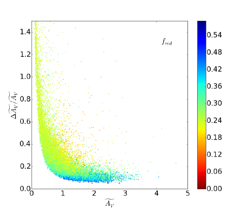
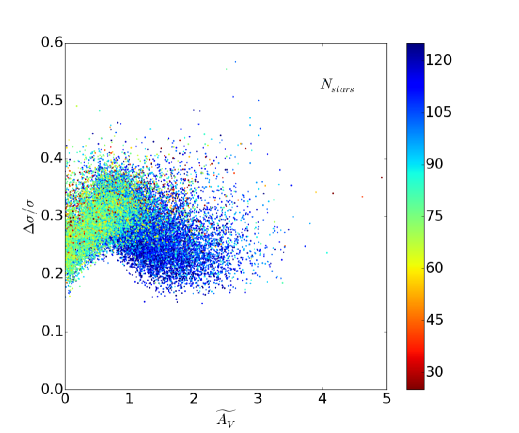
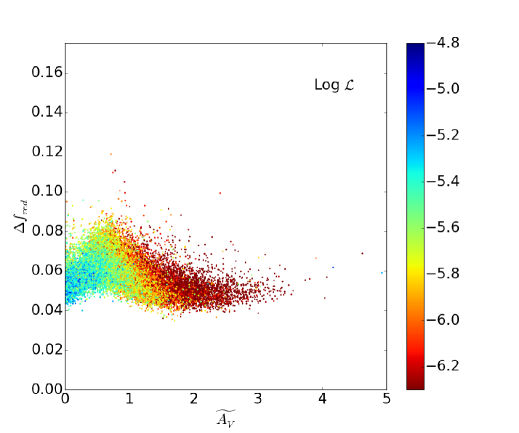
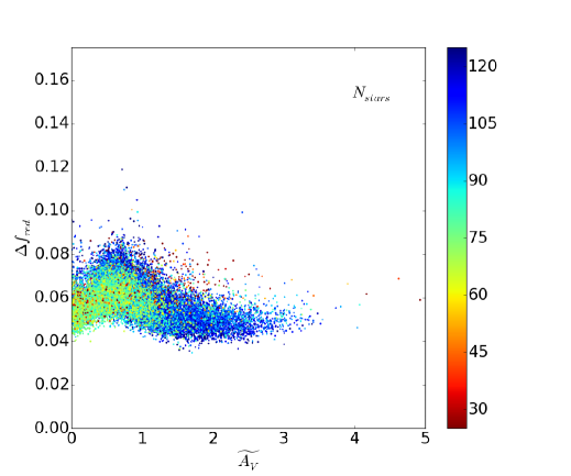
Figure 18.— Uncertainties $\Delta\widetilde{A_{V}}/\widetilde{A_{V}}$, $\Delta\sigma/\sigma$, and $\Delta f_{red}$ (clockwise from top left) as a function of median extinction $\widetilde{A_{V}}$, for each pixel in Brick 16, color-coded by the reddening fraction (upper left), number of stars fit per pixel (right panels) and the log likelihood of the model fit (lower left). As expected from visual inspection of Figure 14, uncertainties increase strongly at low extinctions, where the reddened RGB is not cleanly separated from the unreddened RGB. In regions of modest or high extinction ($>1{\rm\,mag}$), fractional uncertainties are typically lower for the median extinction than for the width of the log-normal. The log likelihood of the best fit decreases steadily with increasing $\widetilde{A_{V}}$ because as the constraining power of the data becomes stronger (as reflected in the smaller uncertainties), any deviations from the assumed log-normal distribution become apparent. The lower right panel shows $\Delta f_{red}$ again, but now color-coded by the number of stars in each pixel. Not unexpectedly, at fixed extinction, the uncertainties are higher when the number of stars is lower.

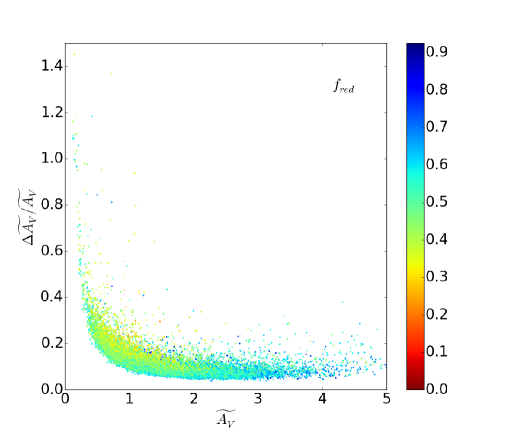
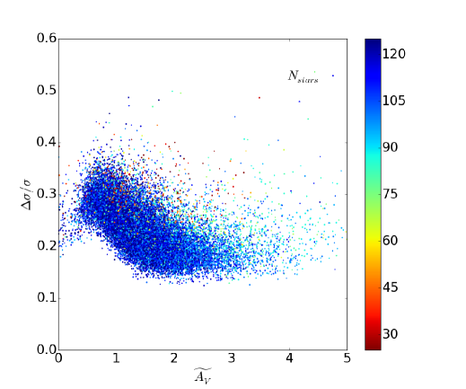
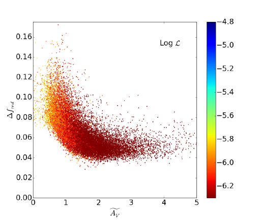
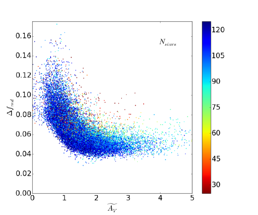
Figure 19.— Same as Figure 18, but for the high extinction star-forming region in Brick 15. Uncertainties $\Delta\widetilde{A_{V}}/\widetilde{A_{V}}$, $\Delta\sigma/\sigma$, and $\Delta f_{red}$ (clockwise from top left) are as a function of median extinction $\widetilde{A_{V}}$, for each pixel in Brick 15, color-coded by the parameter indicated in the upper right of each panel. Given the overall high extinction in this region, the associated uncertainties on the parameters are much smaller than in Figure 18

5.3.1 Failures of Model Fitting

In addition to the normal scatter due to random uncertainties, there are individual pixels where the model fitting has obviously failed. These cases are most noticeable in low extinction regions, where we find occasional pixels that have extremely high values of $\widetilde{A_{V}}$, in a region where there is no other evidence for significant dust. There are two major failure modes we have identified in these regions.

Spurious Photometry & the Noise Model

The first of these cases corresponds to failures of our adopted noise model. If an individual pixel has unusually high contamination from bad photometry, then there will be a larger than expected number of spurious detections. When these sources are not well-represented by our noise model the fitting code will adjust the log-normal parameters to increase the likelihood of finding stars far redward of the RGB, where such spurious sources typically lie (i.e., close to the photometric limit). As a result, the best fit value of $\widetilde{A_{V}}$ and/or $\sigma$ will be driven to large values in an attempt to produce an extremely broad log-normal component, increasing the probability of finding very red sources. This failure represents a complete breakdown of our model. The effect is especially pernicious in regions with low reddening fractions, where one expects few stars redward of the unreddened RGB. It is further compounded in the outer disk, where the absolute number of stars per pixel is small. Luckily, however, these same failure modes are also marked by much higher than average uncertainties in $\widetilde{A_{V}}$, allowing them to be easily identified. An adaptive pixel size would help alleviate this issue, at the expense of complicating comparisons with other dust tracers by introducing spatial variations in the resolution.

Although the noise-model failures sometimes affect only a single isolated pixel, they also sometimes affect multiple adjacent pixels (i.e., spanning $\gtrsim 13\arcsec$). The most common reasons for such highly clustered spurious sources are (1) improper rejection of sources on diffraction spikes around bright stars; and (2) subregions of background galaxies. To minimize the impact of these bad fits in the following analysis, we use unsharp masking to identify pixels that are wildly different from their neighbors, and then replace those pixels with the local median of the neighboring pixels. Our rejection threshold is extremely conservative, and therefore some problem areas clearly remain even in the cleaned maps. All subsequent analysis will use these “cleaned” maps.

WFC3 Calibration Issues

The second failure of the models in low extinction regions is due to the WFC3/IR photometric calibration errors discussed in Sec. 4.1. Inspection of the right hand plot in Figure 6 shows that there are repeating structures in the map of mean RGB color, even after applying the first order correction in Sec. 4.1. These structures follow a square pattern that coincides with the locations of the individual WFC3/IR frames that make up the survey data. This pattern suggests that some of the width of the RGB is due to stars in one part of the detector consistently appearing redder or bluer than stars in another area. As discussed in Sec. 4.1, such an offset could be due to different accuracies in the flat fields used for the F110W and/or the F160W filters, or (more likely) due to systematic differences in the accuracy of the spatially-varying model point spread functions used for photometry. Attempts to track down the exact calibration issue are on-going. We have reduced the effect of these structures on the eventual extinction map by introducing a fitting parameter $\delta_{c}$ to allow very small shifts in the color, but the correction is noisy, particularly when the fraction of unreddened stars is small. Thus, while it helps, residual issues remain.

The pattern is created because our procedure for creating a model of the unreddened stars identifies stars in regions where the RGB is narrow and blue. Regions where the RGB is redder and/or broadened by systematic errors in the photometry will therefore be best fit by models with higher extinction. When these systematically redder and bluer regions are consistently found in certain parts of the WFC3/IR footprint, they imprint a pattern of apparently higher than normal extinction on the resulting map. However, because these photometric issues are at the level $<\pm 0.02{\rm\,mag}$ nearly everywhere, their effects are only noticeable when the extinction is small. We can estimate the amplitude of this effect on the $A_{V}$ map by considering the most extreme case, where all the stars in the model unreddened CMD would come from portions of the WFC3/IR footprint with systematically blue colors. In this case, unreddened regions that lie in the systematically redder parts of the WFC3/IR footprint would by redder by $\lesssim 0.04{\rm\,mag}$, corresponding to an apparent, spurious extinction of $A_{V}\lesssim 0.3{\rm\,mag}$. This amplitude is comparable to the typical random errors at low extinction (Figures 18 and 19). We expect these features to eventually be eliminated in the final version of the PHAT photometry, which will use spatially-variable PSF models in the NIR.

5.3.2 Possible Systematic Uncertainties

The uncertainties derived above are tied specifically to our chosen model. If this model is incorrect, systematic uncertainties can be introduced into our analysis without being reflected in the uncertainties derived from the MCMC fit. We have already addressed several of the systematics inherent in constructing a model of the unreddened CMD (Sec. 4.2.5; i.e., failure to identify true zero reddening stars, biases from population gradients and projection effects, foreground reddening, etc), but address a few additional points here.

Variations in the Reddening Law

We have assumed that there is a single conversion between reddening and extinction that applies throughout M31 (see Sec. 3). This assumption may not hold if there are local departures from a standard $R_{V}=3.1$ extinction law. In such cases we will convert the observed reddening into the wrong extinction. However, the conversion in the NIR is relatively insensitive to the value of $R_{V}$. Even an extreme value of $R_{V}=5$ leads to an inferred extinction that is only 15% different than in the $R_{V}=3.1$ case, which is less than our typical precision. We therefore do not anticipate this to be a significant source of error in the extinction map.

The Assumption of a Log-Normal $A_{V}$ Distribution

Our model assumes that the distribution of extinction in each spatial pixel can be approximated as a single log-normal. If the true distribution is more complex, then the specific values of parameters are harder to interpret and their uncertainties may not be correct.

The log-normal appears to be an adequate representation for the majority of sightlines in typical Milky Way molecular clouds and the diffuse ISM, but the densest star-forming clouds are usually found to have an additional power-law at high-extinctions (e.g., Kainulainen et al., 2009, ; see the more extensive discussion in Sec. 3). In practice, deviations from log-normal distributions are not a large concern, given that the power-law tail is only found in the most actively star forming clouds, and contains only a small fraction of the cloud mass when present. The highest column densities occupy a very small volume of any molecular cloud, and thus random sampling of the column density distribution using background RGB stars will tend to miss any features that occupy only a negligible fraction of the pixel area. The only notable effect may be a tendency of fits to favor a somewhat broader distribution (i.e., larger $\sigma$), particularly in regions with large median extinctions. Inspection of Figures 16 and 17 suggest that this combination of parameter values is not common.

Another violation of the log-normal assumption may occur when the gas distribution is sufficiently complex that there are multiple gas layers along the line of sight. For example, two molecular clouds that are spatially coincident when viewed in projection could have different densities and depths along the line of sight, and thus would produce a more complex reddening distribution than we have assumed. However, even when multiple gas overdensities are superimposed along the line of sight, they are unlikely to all contribute equally to the column density distribution, such that the total reddening distribution is likely to be dominated by the subcomponent with the highest column density with the largest fraction of stars behind it, potentially leaving the log-normal as an adequate fit.

As a potential test of the suitability of the log-normal model, we have color-coded the values of the uncertainties by the log of the posterior probability of the best fit model in Figures 18 and 19. There is an obvious trend such that the log-normal model becomes systematically less likely at higher extinction (although only by $\sim 1.5$ dex). This behavior is not alarming, because our data clearly have less constraining power at low extinctions; when the ability to constrain parameters is low, making it impossible to rule against a given adopted model. Any model is therefore acceptable in terms of the posterior probability of the best fit. While we could engage in more exhaustive testing of whether a log-normal is the optimal functional form, we proceed with an understanding that the log-normal parameters are best interpreted as a good, but approximate, first-order characterization of the distribution of column densities within the pixel.

Biases from Reddened Young Stars

Our model assumes that all of the stars that we fit in the CMD are reddened RGB stars. However, in regions of significant reddening, some of the younger stars that are blueward of our analysis region can be reddened into the portion of the CMD that we are analyzing. These younger stars are typically found in high extinction regions (e.g., Harris et al., 1997; Zaritsky et al., 2002, 2004), making this mechanism a possible source of bias.

Unfortunately, the amplitude of the bias is difficult to quantify because the young stellar populations have much more dramatic spatial variations (Lewis et al., 2015) than the older RGB stars, which have been well-mixed over many dynamical times ($\sim 250{\rm\,Myrs}$ in M31’s main star-forming ring). Thus, the exact degree to which highly reddenened young stars contaminate the RGB analysis region will depend on exactly how numerous the young stars are relative to RGB stars. The degree of contamination will also depend on the ages of the young stars, since the core Helium-burning sequences (roughly 25–$400{\rm\,Myr}$) are redder than the main sequence, and thus can more easily be reddened into our analysis regions. Finally, the degree of contamination will also depend on the depth of the observations. At brighter magnitudes, core Helium-burning stars are well-separated from the RGB, but at fainter magnitudes, they merge into the red clump where their colors are indistinguishable from the main population of RGB stars. In this latter case, reddening of these stars would produce no bias, because they would be included in the unreddened model.

Although the exact amount of bias is difficult to compute, we can make a first order estimate by calculating the colors of stars at different ages, and their relative numbers compared to the RGB. We adopt photometric errors comparable to those in PHAT, and assume a constant star formation rate. Overall, this choice will tend to overestimate the contribution of young stars, given that M31’s star formation rate has declined since a burst 2–$3{\rm\,Gyr}$ ago (Williams et al., 2015). However, Figure 13 of Lewis et al. (2015) shows that there are some star-forming regions that have recent star formation rates (averaged over $100{\rm\,Myr}$ and $\sim\!0.4{\rm\,Gyr}$ timescales) that are of the order of the past average star formation rate or higher. In these regions, the potential bias will be somewhat higher than we estimate here.

In Figure 20 we plot the resulting distribution of colors for 4 different age ranges (100–$500{\rm\,Myr}$, $500{\rm\,Myr}$–$1{\rm\,Gyr}$, $1$–$2{\rm\,Gyr}$, and $>\!2{\rm\,Gyr}$), assuming a modest degree of metallicity evolution ([Fe/H] = 0 for the two most recent bins, -0.25 for the 1–$2{\rm\,Gyr}$ bin, and $-$0.75 in the oldest age bin); the first age ranges encompass the ages probed in Lewis et al. (2015)’s spatially resolved maps of M31’s recent star formation history. We do not include results for ages younger than $100{\rm\,Myr}$, since these stars are too few and too blue to make any significant contribution. We plot the distributions relative to the color of the oldest stellar populations (i.e., relative to the peak of the RGB), for four different magnitude ranges. Each plot lists the numbers of stars redder than $F110W-F160W=0.2$, both as an absolute number and as a percentage of the stars in the oldest RGB peak; these numbers give some sense of the relative size of the young population that might potentially contaminate the RGB when reddened.

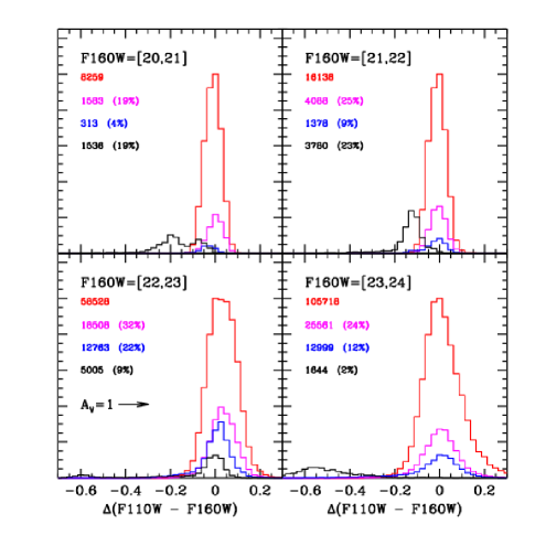
Figure 20.— The distribution of colors for stars in 4 different age ranges (100–$500{\rm\,Myr}$, $500{\rm\,Myr}$–$1{\rm\,Gyr}$, $1$–$2{\rm\,Gyr}$, and $>\!2{\rm\,Gyr}$; black, blue, magenta, and red, respectively), assuming a modest degree of metallicity evolution ([Fe/H]$=\!0$ for the two most recent bins, -0.25 for the 1–$2{\rm\,Gyr}$ bin, and $-$0.75 in the oldest age bin), for a simulated CMD assuming a constant star formation history and typical PHAT photometric errors. Each panel shows the distribution of colors within a $1{\rm\,mag}$ interval of F160W magnitude. To assess the possible contribution of reddened young stars to the RGB-dominated portion of the CMD, all colors are given relative to the peak of the stars in the oldest age range; the arrow in the bottom left panel shows the reddenening expected for $A_{V}=1{\rm\,mag}$ of extinction. The numbers listed in each panel give the number of stars in each histogram; percentages are given relative to the number of stars in the oldest peak. Stars older than $\sim\!500{\rm\,Myr}$ have NIR colors that are indistinguishable from the main RGB peak. Stars in the youngest bin can have bluer colors at young ages, but are not numerous and require large reddening before they could be mistaken as RGB stars with modest reddening.

Figure 20 suggests that the impact of contamination from young reddened stars is likely to be small. Stellar populations older than $\sim\!0.5{\rm\,Gyr}$ have colors that are indistinguishable from the RGB. While their presence or absence may affect the total number of stars in a given pixel, our model fits only relative distribution of stars on the CMD, and is thus insensitive to their presence. Stars in the 100–$500{\rm\,Myr}$ age range will likewise have no impact at faint magnitudes (F160W$>22$) where their fractional contribution is small ($\leq 5$% of the number of RGB stars), and their colors are either indistinguishable from the RGB ($22<F160W<23$), or too blue to make any contribution except at the very highest extinctions ($23<F160W<24$).

At brighter magnitudes ($22<$F160W), the 100–$500{\rm\,Myr}$ stars are proportionally more important. They contain up to 20-25% of the number of stars found in the RGB (assuming a constant star formation rate), and could be reddenened to the color of the RGB peak with 1–$1.5{\rm\,mag}$ of visual extinction. If the young stars experienced this amount of extinction, they would merge with the peak of unreddened RGB stars. The model fits would then assume that the fraction of reddened stars was smaller than it actually was. To affect the measurement of $A_{V}$, however, the stars would need to experience even more reddening, such that they moved redwards of the RGB peak. In this case, the presence of the stars would tend to bias the measurement of $A_{V}$ to lower values. However, given that (1) RGB stars would still outnumber the young stars 3:1 at bright magnitudes; (2) that the fainter stars where the bias is low are factors of 4-6 times more numerous; and (3) that the inclusion of the noise model can potentially “absorb” some fraction of stars that appear abberant compared to the pure RGB fit, it is not clear by how much the best fit model would be biased in practice. We therefore conclude that biases due to reddening from young $<0.5{\rm\,Gyr}$ old stars is likely to be negligible in most cases, and would only potentially be detectable at the highest extinctions ($A_{V}>2$), at anomalously high SFRs in the 100–$500{\rm\,Myr}$ age range, and where the data was shallowest (i.e., in the inner disk).

Loss of Stars at High $A_{V}$

Another possible source of bias would be if highly reddened stars are systematically missing from our data in high extinction regions, due to their suffering enough extinction that they fall below our detection limit. Given the range of extinction found in our analysis, rarely is the extinction high enough to completely remove large numbers of moderately bright RGB stars (e.g., Figure 9). This is not to say that no individual stars have been reddened out of the sample. Intrinsically faint RGB stars are certainly “missing”, and undoubtedly occasional bright RGB stars may be extinguished as well if they happen to fall behind the very smallest, densest core of a molecular cloud. However, it appears highly unlikely that either effect is not being accounted for in the model fitting, as long as the mode of the log-normal distribution is detectable for some of the RGB.

Summary of Systematic Biases

All of the potential systematic biases identified above and in Sec. 4.2.5 are modest ($A_{V}\lesssim\!0.3{\rm\,mag}$) or confined to very rare regions. Systematic errors are therefore likely to only be noticeable at low extinctions. However, the random errors at these low extinctions are large, so that the systematic errors may not actually dominate the error budget for any individual pixel. However, the effects of systematics can be noticeable when looking at the cumulative behavior of the extinction over large, low extinction regions of the galaxy, which essentially averages over many pixels and thus reduces the impact of random uncertainties. We look for evidence of these effects in Sec. 6.4 below, after presenting our final dust maps and comparing them with other measurements of dust extinction.

6. Results

6.1. A Galaxy Wide Map of M31’s Cool ISM

In Figure 21 we present the full maps of M31’s median extinction $\widetilde{A_{V}}$. Figures 22–24 show a series of zoomed in regions of the same maps, from the inner to the outer disk (i.e., moving from bottom to top in Figures 21). All images show the full interleaved map (12.5${\rm\,pc}$ pixel sampling with 25${\rm\,pc}$ resolution). We present only the cleaned maps; some remaining spurious features due to high numbers of false detections near bright stars are still visible, particularly in the outer disk. There are also very low level “grid” structures due to the $\pm 0.01{\rm\,mag}$ structured systematics in the photometry across the WFC3/IR chip (as discussed in Sec. 4.1 and 5.3.2).

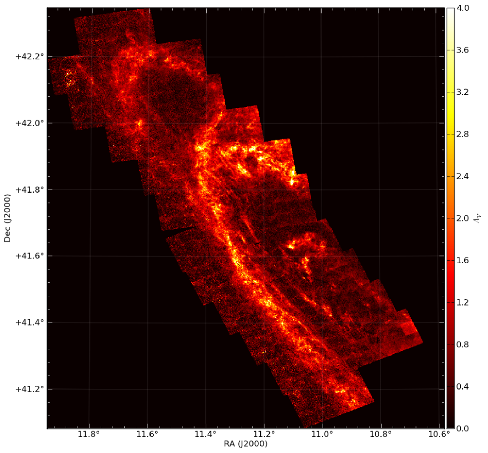
Figure 21.— Map of the median extinction $\widetilde{A_{V}}$ for all analyzed regions. Some very low-level “grid” patterns are visible in the map, due to position-dependent calibration issues with the WFC3/IR chip (Sections 4.1 & 5.3).

The maps in Figures 21—24 reveal extremely rich details. Assuming that the extinction is proportional to the column density of cold gas, the maps of $\widetilde{A_{V}}$ offer one of the highest resolution views of the ISM of a spiral disk, outside our own Milky Way. The structure of the extinction shows networks of filaments (Figures 23 & 24), holes (Figure 23), ripples/feathers (Figure 22; seen as repeating hooked structures on the inside edge of major star-forming ring), and spurs (Figure 24; linear features extending radially from the major star-forming rings and spiral arms). These latter two features are thought to be direct results of hydrodynamic instabilities (e.g., Kim & Ostriker, 2002; Chakrabarti et al., 2003; Shetty & Ostriker, 2006; Kim & Ostriker, 2006; Dobbs & Bonnell, 2006; Lee & Shu, 2012), making the maps a superb resource for understanding these common features of spiral disks (e.g., Elmegreen, 1980; La Vigne et al., 2006). For example, the regular pattern of spurs evident in the inside edge of M31’s star-forming ring (Figure 22) has a particularly small opening angle, and quickly bends around to form almost a complete inner ring. In contrast, simulations of spur formation typically find much more open patterns of spurs than are seen here.

Inspection of Figure 21 shows that typical extinctions are of order $\widetilde{A_{V}}\!\sim\!1$, with very little surface area having $\widetilde{A_{V}}\!>\!3$. If we limit the map to only those regions with well-measured values of $\widetilde{A_{V}}$ (fractional errors $\Delta\widetilde{A_{V}}/\widetilde{A_{V}}\!\lesssim\!0.3$), the median of $\widetilde{A_{V}}$ is $1.0{\rm\,mag}$, with only 10% of the pixels having $\widetilde{A_{V}}\!>\!1.8$, and 1% having $\widetilde{A_{V}}\!>\!2.8$. For comparison, the Milky Way sample of 23 molecular clouds studied by Kainulainen et al. (2009) has a median of $\widetilde{A_{V}}\!=\!1.2$, and only 2 clouds have $\widetilde{A_{V}}\!>\!3$. Thus, although one cannot draw firm statistical conclusions based on the heterogeneous Kainulainen et al. (2009) sample, the median extinctions in M31 are not obviously atypical for what is seen locally in the Milky Way.

Figure 22.— Map of the median extinction $\widetilde{A_{V}}$ for the inner regions containing Bricks 2, 4, 6, and 8 along the $10{\rm\,kpc}$ star-forming ring (bottom to top), and the major axis field Brick 5, which samples a smaller, less intense star-forming ring. Note the regular ripples or spurs along the inside edge of the star-forming ring.

Figure 23.— Map of the median extinction $\widetilde{A_{V}}$ for: (1) the major axis of the the $10{\rm\,kpc}$ star-forming ring (Bricks 12, 14, and 16 along the left, and Bricks 15 and 17 along the major axis, from bottom to top); (2) the major axis field Brick 9, which samples the second of the 2 inner star-forming rings; and (3) the star of the outermost star-forming ring (Brick 18, in the upper left). The ripples/spurs noted in Figure 22 continue into Brick 12 on this map.

Figure 24.— Map of the median extinction $\widetilde{A_{V}}$ in the outer disk, including Bricks 17, 19, 21, and 23 along the major axis, and Bricks 18 and 22 on the left of the image. Two of the fields in Brick 22 (near $\alpha=11.86^{\circ}$, $\delta=42.14^{\circ}$) have somewhat higher-than-expected photometry errors, which leads to a large fraction of erroneous pixels in the dust map.

One way to assess the veracity of the extinction maps is to compare to other tracers of extinction. A straightfoward test is to compare the dust morphology to that seen in optical imaging in blue filters. At these wavelengths, dusty structures can appear as dark features against the smooth background of unresolved stars, albeit with confusion from foreground stars. Optical images also have the highest spatial resolution of various extinction tracers.

In the lower right panels of Figures 25—27, we show blue optical images of the same regions as the extinction maps in Figures 22, 23, and 24 (reproduced in the upper left of Figures 25–27, for reference). The extinction features seen in our maps rival the resolution of the equivalent features seen in the optical images. The morphology of the features are in excellent agreement as well.

As a further morphological comparison, the lower left panels of Figures 25—27 show the publicly available Westerbork maps of Hi from Brinks & Bajaja (1986). Although these maps have significantly lower resolution ($45\arcsec$) than the extinction maps, the broad morphology is again in good agreement.

While the comparison between the optical image and the extinction map show many of the same detailed structures, the new extinction maps offer a far less ambiguous view. First, they lack the complicated foreground of young stars that confuses interpretation of extinction features in broad-band images. But more importantly, the new maps measure the total extinction of the dust column, regardless of where it is with respect to the stars. In contrast, there are extinction features in the broad-band optical image which appear extremely strong, when in fact the strength results only from the dust layer being closer to the foreground, allowing it to block more of light due to geometry alone. A clear example of this effect can be seen in the optical image in Figure 25, where the structure at ($10.92^{\circ}$, $41.42^{\circ}$) appears to be much higher column density than the neighboring structure at ($10.99^{\circ}$, $41.45^{\circ}$). Comparing to the adjacent map of $\widetilde{A_{V}}$, however, reveals that the latter clump is actually the higher extinction region. Instead, the high apparent extinction is due primarily to the much higher reddening fraction in that region. This example points to the peril of using color and/or unsharp masking to infer the extinction from maps of the attenuation (e.g., Regan et al., 2011), particularly in inclined galaxies with large variations in $f_{red}$.

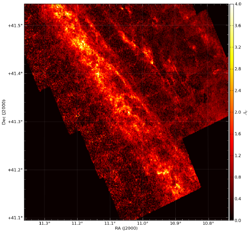
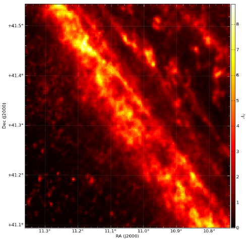
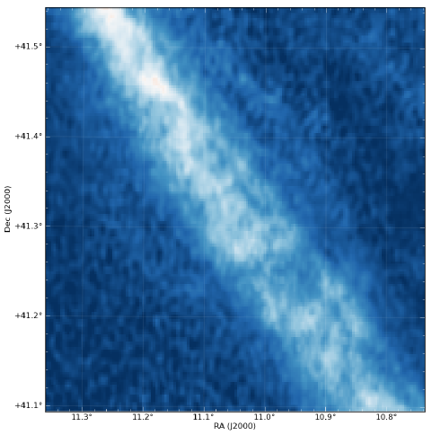
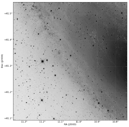
Figure 25.— Comparison between the new M31 extinction map ($\widetilde{A_{V}}$; upper left), the extinction inferred from the emission-based Draine et al dust map (upper right), an Hi map (lower left), and an optical image (lower right). These maps reproduce the area shown in Figure 22.

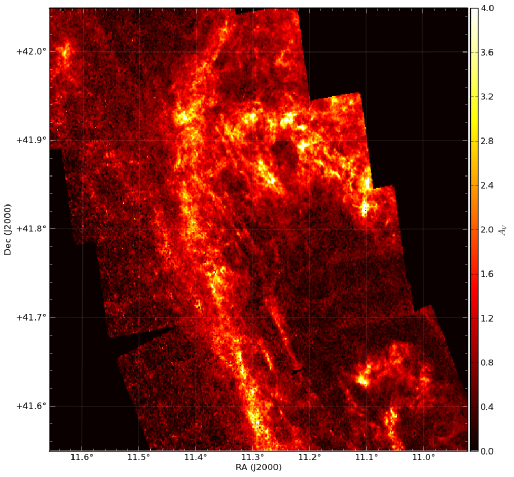
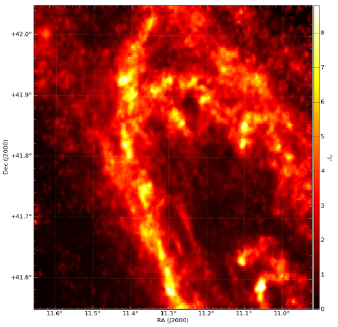
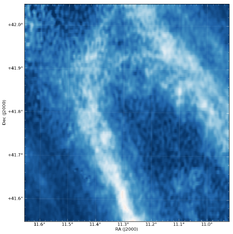
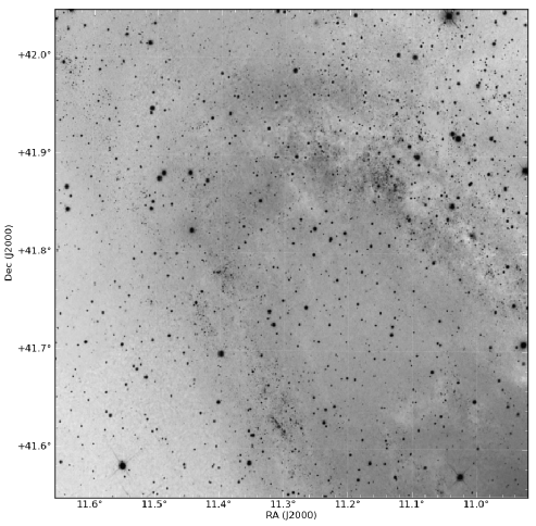
Figure 26.— Comparison between the new M31 extinction map ($\widetilde{A_{V}}$; upper left), the extinction inferred from the emission-based Draine et al dust map (upper right), an Hi map (lower left), and an optical image (lower right). These maps reproduce the area shown in Figure 23.

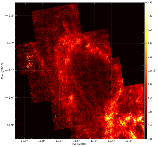
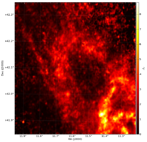
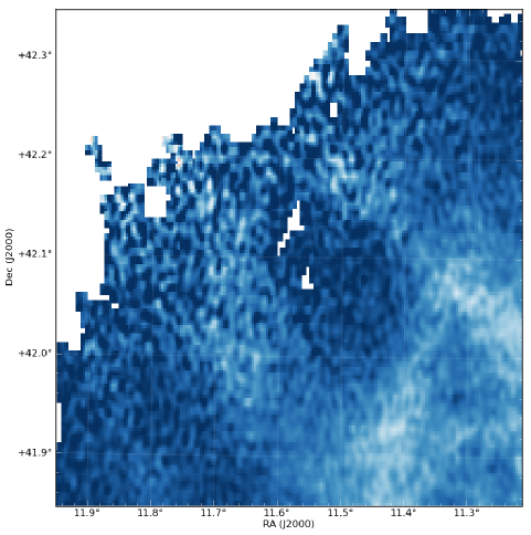
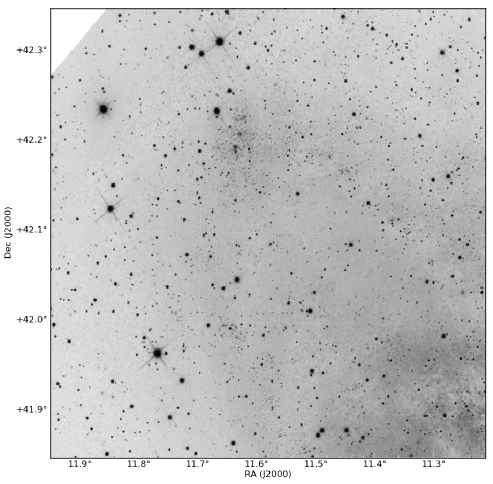
Figure 27.— Comparison between the new M31 extinction map ($\widetilde{A_{V}}$; upper left), the extinction inferred from the emission-based Draine et al dust map (upper right), an Hi map (lower left), and an optical image (lower right). These maps reproduce the area shown in Figure 24.

6.2. Comparison with Emission-Based Maps of Dust Mass

Thanks to revolutionary new mid- and far-infrared facilities (e.g., Spitzer, Herschel), and sophisticated models (e.g., Desert et al., 1990; Draine & Li, 2007; Compiègne et al., 2011), it has now become standard to use long-wavelength spectral energy distributions (SEDs) to infer the mass, composition, and temperature of the dust, and the illuminating radiation field (e.g., Tuffs et al., 2004; Boissier et al., 2004; Walter et al., 2007; Muñoz-Mateos et al., 2009; Noll et al., 2009; Montalto et al., 2009; Dunne et al., 2011; Boselli et al., 2010; Smith et al., 2010; Compiègne et al., 2010; Tamura et al., 2010; Popescu et al., 2011; Galametz et al., 2011; Skibba et al., 2011; Galliano et al., 2011; Dale et al., 2012; Bendo et al., 2012; Aniano et al., 2012; Smith et al., 2012; Galametz et al., 2012; Groves et al., 2012). In nearby, well-resolved galaxies, these techniques can generate maps of the dust mass as a function of position, which, for a given dust model, can be converted directly into predictions for the extinction.

Recently, Draine et al. (2014) published a state-of-the-art analysis of M31’s dust, using emission maps from Spitzer’s IRAC and MIPS cameras (Barmby et al., 2006; Gordon et al., 2006, respectively), and from high resolution HERSCHEL maps made with PACS and SPIRE (Groves et al., 2012). The SEDs cover from 3.6$\mu$m to $\sim$500$\mu$m, using observations in 13 different bandpasses. The resulting maps of the dust column density were generated at two resolutions: 24.9$\arcsec$ and 39$\arcsec$, corresponding to the resolution of the SPIRE $350\mu$m and the MIPS $160\mu$m observations, respectively, and then sampled with either 10$\arcsec$ or 16$\arcsec$ pixels. A high ($6\arcsec$) resolution emission map has also been published by Montalto et al. (2009), but the level of contamination from stellar sources makes it difficult to compare to the work here.

The emission-based dust map of Draine et al. (2014) can be used to make a direct prediction for the extinction. Draine et al. (2014) derive the extinction-to-dust mass surface density ratio $A_{V}/\Sigma_{Md}=7.394$ for their specific model of the dust composition, where $\Sigma_{Md}$ is the dust mass surface density in ${\rm\,M_{\odot}}/{\rm\,pc}^{2}$.

In the upper right of Figures 25—27, we plot the predicted distribution of $A_{V}$ derived from the 24.9$\arcsec$ resolution Draine et al. (2014) dust map (i.e., $A_{V,emission}$). The morphological agreement between the $A_{V,emission}$ map and the CMD-based $\widetilde{A_{V}}$ map is superb, particularly in regions where $\widetilde{A_{V}}\gtrsim 1{\rm\,mag}$. Even very small features are clearly reproduced in both of the maps, in spite of their completely independent derivations. It is hard not to see the level of agreement as a triumph for both techniques.

That said, the maps do present some differences. The CMD extinction maps have nearly 4 times the spatial resolution ($93{\rm\,pc}$ vs $25{\rm\,pc}$), which naturally produces clearer views of the smallest features. However, the emission-based maps will be sensitive to any dust in a given pixel, whereas the CMD extinction-based maps can miss dust that is locked into small dense structures with negligible filling factors. The emission-based maps are also possibly more accurate at low extinctions, where the CMD-mapping technique is limited by our ability to: (1) detect broadening over the intrinsic width of the RGB; and (2) generate accurate “zero-reddening” models of the RGB. On the other hand, the emission-based maps face their own difficulties at low extinctions, where the uncertainty in wide-field background subtraction and calibration can easily produce large-scale systematic offsets in the photometry. Emission maps may also have difficulty disentangling emission from unresolved dust components with different temperatures (e.g., Galliano et al., 2011).

The most glaring discrepancy between the two techniques is the offset in the normalizations. Examination of the color scales in Figures 25—27 shows that the emission-based maps predict extinctions that are more than twice those that are observed. This difference is present even in low extinction regions, suggesting that it cannot be due to simply missing very dense dust clouds with very small filling factors, which would only affect the highest column density regions. Given the simplicity of the CMD-based extinction technique compared to the emission based technique (which relies on assumptions about the radiation field as well as calibrations within the Milky Way; e.g., Weingartner & Draine, 2001), it is far more likely that this global offset represents an issue with the current calibration of the dust emission models.

We make a more quantitative assessment of this offset by comparing a resolution-matched version of our CMD-based extinction map to the emission-based map. We use the mean extinction $\langle A_{V}\rangle$ for all comparisions, rather than the median $\widetilde{A_{V}}$; these two quantities can be significantly different for a log-normal distribution, and the mean is the better estimate of the total dust column density and thus is a fairer test of the quantity tracked by the emission-based map. We extract the posterior probability distribution function of $\langle A_{V}\rangle$ directly from the MCMC samples, rather than deriving it from the combination of the best fit $\widetilde{A_{V}}$ and $\sigma$ (i.e., $\langle A_{V}\rangle=\widetilde{A_{V}}\exp{(\sigma^{2}/2)}$; Eqn. 6); this choice avoids any biases due to correlations between $\widetilde{A_{V}}$ and $\sigma$. We then degrade the resolution of the $\langle A_{V}\rangle$ map from ${\rm FWHM}=6.645\arcsec$ to ${\rm FWHM}=24.9\arcsec$ by smoothing with a Gaussian kernel of standard deviation of 10.19$\arcsec$ ($=\sqrt{24.9^{2}-6.645^{2}}/2\sqrt{2\ln{2}}$); this degrades the resolution from $25{\rm\,pc}$ to $94{\rm\,pc}$. We use this resolution-matched map of $\langle A_{V}\rangle$ in all subsequent comparisons with results from Draine et al. (2014).

The top left panel in Figure 28 shows the pixel-by-pixel correlation between the Draine et al. (2014) extinction maps and the mean extinction $\langle A_{V}\rangle$ of the reddened component, derived from the NIR CMD. The pixels are highly correlated, as expected from the excellent morphological agreement seen in Figures 25—27. However, it is clear from the top left of Figure 28 that the extinctions from the Draine et al. (2014) maps are higher by a factor of $\gtrsim$2. There is also a small tail of points where there is little dust emission, but the CMD-based extinction is higher. These points are all due to regions where the photometry is slightly biased to redder colors near the chip edge in the very outer disk, where there are other photometry errors (Fields 2 and 8 of Brick 22), or where crowding is high and the RGB is intrinsically broad in the very inner disk (Fields 3 and 4 of Brick 3).

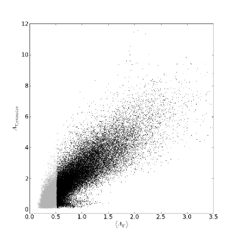
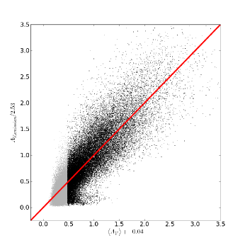
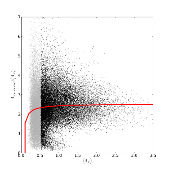
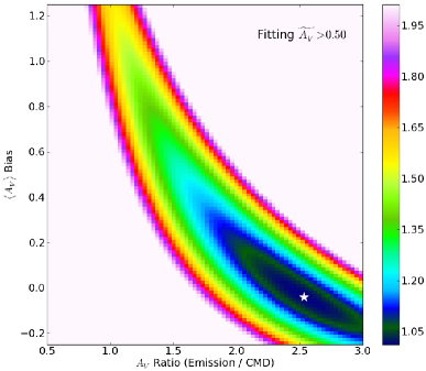
Figure 28.— (Top Row) Pixel-by-pixel comparisons between the Draine et al. (2014) emission-based $A_{V}$ map and the resolution-matched map of mean extinction $\langle A_{V}\rangle$ derived from the NIR CMD. The original comparison (left) shows strong correlations, as expected from the morphological agreement. However, the steep slope and the vertical offset from the origin indicate issues with the overall scaling between the two methods, and a bias in the CMD-based extinction maps at low dust column. After correcting the Draine et al. (2014) maps (right) by an overall scaling factor of $R=2.53$, and correcting the CMD-based extinction by an additive bias factor of $b=-0.04$, the agreement between the two maps is much improved. The scatter is still significant, however. (Bottom Left) The pixel-by-pixel ratio between the two maps and the resolution-matched map of mean extinction $\langle A_{V}\rangle$ derived from the NIR CMD. The red line shows the predicted ratio using the scale$+$bias correction used in the center panel. The results are similar if the median extinction of the reddened component is used instead of the mean, although the scale factors are slightly different. (Bottom Right) The $\chi^{2}$ distribution of the values of the scale factor correction $R$ to the Draine et al. (2014) map and the bias correction $b$ to the CMD-based map, derived where $\widetilde{A_{V}}>0.5$.

6.2.1 Correcting the Emission- and CMD-based Extinctions

We quantify the differences between the emission-based and CMD-based extinction maps by calculating a transformation that would bring the maps into agreement. We assume that the Draine et al. (2014) extinctions are too high, and must be divided by a factor $R$. We include an additional correction factor $b$ for possible systematic biases in the CMD-based extinctions (see Sec. 4.2.5 & 5.3.2). We then estimate appropriate values for $R$ and $b$ by calculating $\chi^{2}$ on a grid of $R$ and $b$, where $\chi^{2}$ is calculated using the observed ratio $A_{V,emission}/\langle A_{V}\rangle$ compared to the prediction for the model as a function of $\langle A_{V}\rangle$ (i.e., $A_{V,emission}/\langle A_{V}\rangle=R(1+b/\langle A_{V}\rangle)$; lower left of Figure 28). When calculating $\chi^{2}$, we use an empirical estimate of the uncertainty in the measured ratio as a function of $\langle A_{V}\rangle$, since we lack a realistic noise model for the ratio $R$. We limit the calculation to only points with $\widetilde{A_{V}}>0.5{\rm\,mag}$ where measurements for both dust models are expected to be more robust.

The resulting $\chi^{2}$ distribution is shown in the lower right panel of Figure 28. The best-fit model parameters are $R=2.53$ and $b=-0.04\,{\rm mag}$ when using the mean CMD-based extinction $\langle A_{V}\rangle$. If the CMD-based extinctions are assumed to be unbiased ($b=0$) then the scaling for the Draine et al. (2014) extinctions shifts to slightly lower values of $R$.

In the upper right panel of Figure 28, we show the pixel-by-pixel correlation after applying these corrections, such that $A_{V,emission}\rightarrow A_{V,emission}/R$ and $\langle A_{V}\rangle\rightarrow\langle A_{V}\rangle+b$. The prediction for the ratio using the same model is also shown as the red line on the lower left panel. The overall distribution now has the desired slope of 1 (red line) and is consistent with passing through (0,0).

The fits shown in Figure 28 suggest that (1) there is a negligible global bias in the CMD-derived extinction values, corresponding to a color shift of $\sim\!0.005$ magnitudes in $F110W-F160W$, and (2) there is a large scaling difference between the emission- and CMD-based extinctions. We now discuss the second of these conclusions in more detail, and defer the less pressing issue of biases to Sec. 6.4.

6.2.2 Are the Draine et al. (2014) Extinctions Really Too High?

Figure 28 strongly suggests that there is a factor of $\sim\!2.5$ difference between the extinction inferred from CMD fitting and that inferred from modeling the IR emission. The distribution of $\chi^{2}$ values in Figure 28 shows there is no reasonable value of the bias for which the ratio $R$ becomes 1. Thus, we are in the uncomfortable position of accepting a large systematic problem in either the CMD-based extinction or in widely used models of dust emission.

We argue that the factor of 2.5 scaling difference is more likely to have resulted from a problem with the Draine et al. (2014) emission-based maps. Simply put, there is no obvious way that the extinction inferred from the CMD can have mistaken the degree of reddening by such a large factor. We demonstrate this in Figure 29, which shows the CMD of the same region plotted in Figure 11. The underlying density map shows the CMD expectation for the true best fit model (upper left) and for a model where the true reddening is $\sim$2.5 times higher than what we derived (shown in the lower row as an adjustment to the median extinction $\widetilde{A_{V}}$ or to the width of the distribution, on the left and right, respectively). A higher extinction is completely at odds with the actual observations.

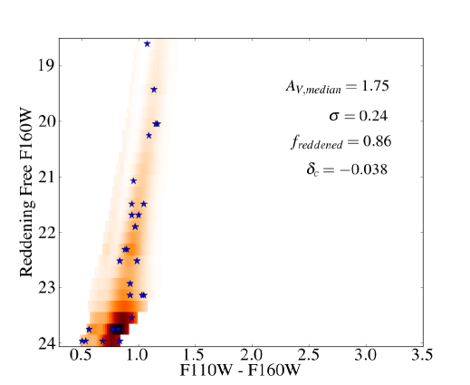
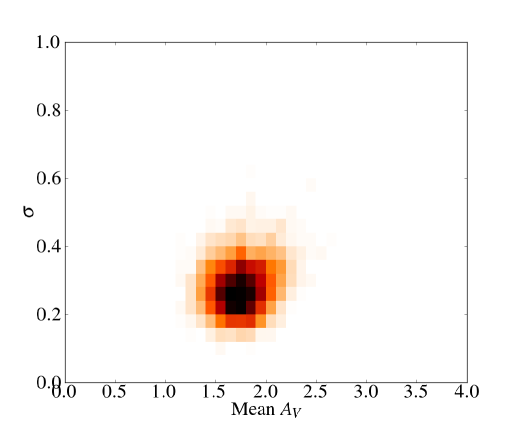
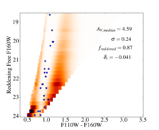
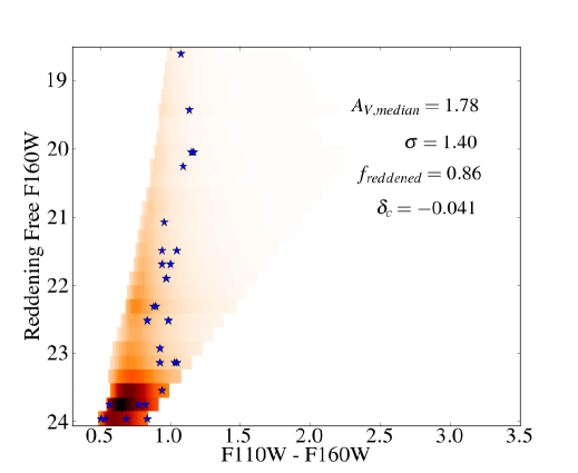
Figure 29.— Binned CMD showing the reddened model derived for stars found in a $25{\rm\,pc}$ pixel in Brick 15 (as in the right panel of Figure 11). The upper row shows the actual best fit model derived from CMD fitting (left) and the joint probability distribution for $\langle A_{V}\rangle$ and $\sigma$ (right). The lower row shows example models corresponding to a factor of 2.53$\times$ higher mean extinction, as inferred from the Draine et al. (2014) dust emission model, made by rescaling the median extinction (left) or the width of the reddening distribution (right). Clearly, the data (shown as blue stars) are not consistent with the higher mean extinction characteristic of the emission-based dust model. Note: slight differences in the best fit parameter values given on each plot are due to difference instances of fitting the same pixel.

The only ways out of this conclusion are deeply unsatisfying. For the CMD-based extinctions to be artificially low at essentially all pixels, we would have had to (1) mistaken the true location of the unreddened CMD by many tenths of a magnitude, or (2) invoked a reddening law with a drastically different relationship between attenuation and reddening in the NIR. We can rule out the first escape route because we have many regions where the vast majority of stars are unreddened (i.e., small $f_{red}$); in these regions, the NIR RGB is essentially exactly where our model places it, and is fully consistent with theoretical isochrones. Moreover, such a color offset would manifest as a constant bias factor, not a difference in scaling. The second solution is equally difficult to accept. While reddening laws are known to vary in the ultraviolet (e.g., Gordon et al., 2003), there is no evidence for significant variations in the NIR at the required amplitude.

In contrast to the difficulty explaining a large scale error in the CMD-based extinctions, there are many possible ways to explain scale errors in the emission-based extinction maps. Converting the spectral energy distribution of the dust emission to a prediction for the extinction requires calculating the dust mass in the context of a specific model for the physical properties of the dust (composition, grain size distribution, etc) and for the starlight radiation field. The Draine et al. (2014) dust map is derived using the Draine & Li (2007) models, which are calibrated to match the emission of diffuse, dusty regions in the Milky Way (e.g., Weingartner & Draine, 2001), with additional adjustments in the volume of grain material to give better consistency with depletion measurements of the dust mass per hydrogen atom (Draine et al., 2014). Given the complexity of the models and the calibration, it is possible that these locally calibrated models do not apply in a different environment. Indeed, Draine et al. (2014) specifically raises the possibility of their systematically overestimating the dust mass when discussing differences with Planck emission, although they argue that systematic errors initially appear smaller than a factor of $\sim$1.3.

Additional complications arise from the degeneracy inherent in fitting dust models to spectral energy distributions, and from the inability to fully resolve complex, multi-temperature dust distributions (e.g., Galliano et al., 2011). Dust emission is highly non-linear with temperature, and thus the ensemble emission from a collection of dust clouds with varying temperatures does not accurately reflect the mean mass-weighted temperature. There is also evidence that cold dust may be much more emissive than expected (Paradis et al., 2009). If the component of high-emissivity dust is pervasive in M31 as well as the MW, then it may help to explain why the Draine et al. (2014) map infers more extinction than is actually seen. However, this effect seems restricted to the molecular phase, which is not dominant in M31.

Comparable mismatches between extinction and the Draine & Li (2007) models have been seen before in the literature. Both Alton et al. (2004) and Dasyra et al. (2005) found that multiwavelength radiative transfer modeling of edge-on galaxies underpredicts the observed sub-mm emission at 850$\mu$m when using the Draine & Li (2007) models. In other words, to be consistent with the observed amount of extinction, either there must be another component of dust not accounted for in their radiative transfer model, or the dust must produce a factor of $\sim$3-4$\times$ greater emission at long wavelengths than predicted by the Draine & Li (2007) model. The inverse of this latter possibility — i.e., that a given amount emission can be produced by 1/3 the amount of dust – would be consistent with our results, after including the model revisions in Draine et al. (2014). Recent simulations, however, suggest that the mismatch may instead be due to asymmetries and inhomogeneities in the disk that affect the outcome of radiative transfer calculations (e.g., Saftly et al., 2015).

Even more clearly, recent work by Plank Collaboration et al. (2014) showed a nearly identical discrepancy to the one we identify here. They measured the optical extinction observed towards thousands of QSOs observed with the Sloan Digital Sky Survey and compared it to the extinction predicted by fitting (Draine & Li, 2007) models to all-sky data from Planck, IRAS, and WISE. This comparison found that the Draine & Li (2007) extinction estimates were too high by a factor of $\sim\!2-2.4$. They found a comparable discrepancy when looking at molecular clouds whose NIR extinctions were mapped using 2MASS by Schneider et al. (2011). We compare our results to those in Plank Collaboration et al. (2014) in more detail in Sec. 6.5 below.

Finally, Lombardi et al. (2014) find a factor of $\sim$2 difference between observations in Orion and the Weingartner & Draine (2001) predictions for the ratio of 2.2$\mu$m extinction to the 850$\mu$m opacity. They argue that this discrepancy is reduced with recent models by Ormel et al. (2011). Interestingly, however, the ratio measured by Plank Collaboration et al. (2014) is actually in much better agreement with Weingartner & Draine (2001), in spite of showing a siginificant difference between the measured and the predicted extinctions from the similar Draine & Li (2007) models.

In summary, it appears that the most widely used Draine & Li (2007) dust models overestimate the mass of dust needed to produce a given amount of emission in M31, even after revising the dust masses downwards using the modifications in Draine et al. (2014). This discrepancy is particularly troubling, given the ever growing importance of dust modeling in the era of flagship mid- and far-IR observatories. Further application of CMD-based extinction measurements outside the Milky Way will be invaluable in improving existing dust models.

6.3. Small-Scale Variations in Emission- and CMD-based Extinctions: The Impact of the Interstellar Radiation Field

In Figure 30 we plot the ratio between the emission-based $A_{V}$ from Draine et al. (2014) and the CMD-based mean extinction $\langle A_{V}\rangle$, after smoothing the latter to match the resolution of the former. The left panel plots the raw ratio, and the right panel plots the ratio after correcting the Draine et al. (2014) extinctions by a factor of $R=2.53$ and the CMD-based mean extinctions by an offset $b=-0.04{\rm\,mag}$. The dark contour shows the locus within which $\langle A_{V}\rangle\!>\!1$ in the smoothed map; CMD-based extinctions outside this locus will potentially be subject to larger systematic uncertainties. The redder regions of the right hand panel indicate regions where the mismatch between the Draine et al. (2014) and the CMD-based extinctions are larger. In the bluer regions the agreement is better, but only approaches good agreement ($A_{V,emission}/\langle A_{V}\rangle\!\sim\!1$ in the left panel) at the very lowest extinctions, where both methods agree there is very little dust.

Figure 30 shows an amount of scatter consistent with that seen in the pixel-by-pixel correlations shown in Figure 28. However, it also shows that the deviations from the mean ratio are often spatially coherent. In the following section (6.4) we assess the possible contribution from systematic errors in the CMD-based extinctions, but before doing so we discuss how such behavior could also be produced by emission-based extinction measurements.

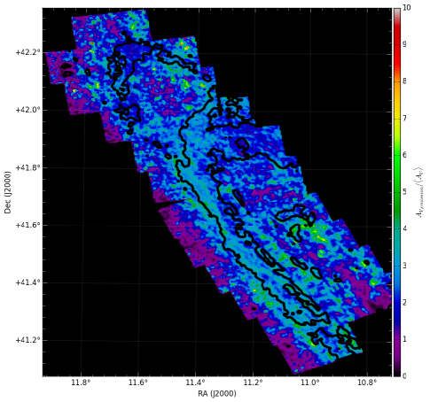
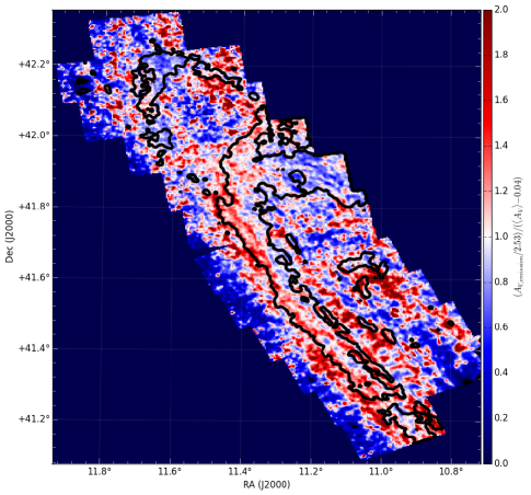
Figure 30.— Images of the pixel-by-pixel ratio of the Draine et al. (2014) emission-based $A_{V}$ map divided by the resolution-matched map of mean extinction $\langle A_{V}\rangle$ derived from the NIR CMD, before (left) and after (right) applying the scale$+$bias correction used in the top-right panel of Figure 28 (Sec. 6.2.1). The heavy dark contours indicate where $\langle A_{V}\rangle>1$. Inspection of the uncorrected map shows that the mismatch between the two maps is clearly spatially dependent. The overall difference in scale in the high extinction regions falls between 2-3, with some tendency towards higher values on the far side of the disk. The scale correction brings the agreement to roughly $\pm 30\%$ in regions with $\langle A_{V}\rangle>1$. The ratio deviates most strongly from 1 at low to intermediate extinctions, due to the expected systematic underestimates in the CMD-based extinctions (discussed in Sec. 5.3); the agreement in these regions is greatly improved by the correction of an additive bias factor, although at the cost of worse agreement at the very lowest extinctions. The correction is not as effective as in the high extinction regions, most likely because the bias factor would be expected to vary radially.

Non-linearities in Smoothing

To produce Figure 30 we have smoothed the CMD-based dust map. However, this smoothing is weighted by the column-density of the dust. In contrast, the smoothing that takes place during emission observations is flux-weighted. The emission from dust is a strong power of dust temperature, and thus the resolution of a mid- or far-IR telescope will effectively smooth the dust map non-linearly, with more weighting given to regions with higher dust temperatures. This can lead to emission maps missing cold dust (e.g., Galliano et al., 2011), and producing systematic mismatches with the observed extinction when there are strong, sharp gradients in the dust temperature. This latter situation is likely to be found on the edges of star-forming regions, such as just beyond the boundaries of the star-forming ring (see Figure 9 of Draine et al., 2014). Such an effect could be responsible for the more significant deviations (redder colors) frequently seen just outside the $\langle A_{V}\rangle\!=\!1$ contour.

Variations in Dust Composition

Models of dust emission typically allow the dust composition, and in particular the polyaromatic hydrocarbon (PAH) content, to vary spatially. Draine et al. (2014) fit for PAH abundance $q_{pah}$ and find strong spatial variations in and out of M31’s star-forming rings, as well as large gradients within the galaxy. Some of the abundance variations are lessened when variations in the interstellar radiation field are also included, particularly in the inner galaxy, but the change in PAH abundance across major star-forming features appears to persist in the more structured northern half of the galaxy. Interestingly, the largest red region outside the $\langle A_{V}\rangle\!=\!1$ contour is also a region where the PAH abundance appears anomalously high for such a low column density region (Figure 11 of Draine et al., 2014). It may be possible that coherent variations in the inferred dust composition may be propagating into coherent variations in the dust extinction. It would not be surprising if M31’s dust composition varied systematically between the diffuse gas in the low column density regions and the denser gas in high column density regions. It is also possible that some of the bias factor $b$ that we have ascribed to the CMD-fitting method may instead be a systematic in how the dust composition changes in the more diffuse ISM. We return to the issue of possible PAH correlations in Sec. 6.5.

The Spectrum of the Interstellar Radiation Field

One of the most interesting features in Figure 30 is the presence of two large regions at high extinction where the ratio $A_{V,emission}/\langle A_{V}\rangle$ is much lower than typical – one in the $10{\rm\,kpc}$ star-forming ring just west of the major axis, and one in the outermost spiral arm along the major axis. These two regions are the locations of two well-known recent star formation events. They can clearly be seen in Figure 13 of Lewis et al. (2015), which plots the “Scalo $b$” parameter, defined as the current star formation rate ($SFR$) divided by the past average SFR. This parameter is closely associated with the hardness of the underlying spectrum. As the Scalo $b$ parameter increases, so does the fraction of young stars, which will increase the contribution from hot stars to the underlying interstellar radiation field, potentially changing the efficiency of dust heating for a given bolometric energy density in the interstellar radiation field.

To explore a possible empirical correlation between the spectrum of the underlying stars and the spatial variation of $A_{V,emission}/\langle A_{V}\rangle$, in Figure 31 we plot the observed ratio of dust extinctions as a function of the Scalo $b$ parameter ($=SFR_{100}/\langle SFR\rangle$) where the “current” star formation rate $SFR_{100}$ is integrated over the past $100{\rm\,Myr}$ using the spatially-resolved recent star formation history derived in Lewis et al. (2015), derived on 100 pc bins. We also plot a rolling average constructed by taking the mean of 200 sequential points ranked by the Scalo $b$ parameter. We restrict this comparison to regions where $\langle A_{V}\rangle\!>\!1$, which should better sample the denser neutral and molecular ISM.

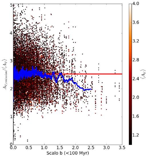
Figure 31.— The observed pixel-by-pixel ratio of the Draine et al. (2014) emission-based $A_{V}$ map divided by the resolution-matched map of mean extinction $\langle A_{V}\rangle$ derived from the NIR CMD (i.e., Figure 30), as a function of the Scalo $b$ parameter ($\equiv\!SFR_{100}/\langle SFR\rangle$) from Lewis et al. (2015). The ratio is systematically smaller as the contribution from hot young stars increases, shown as the running average plotted in blue. For $SFR_{100}/\langle SFR\rangle\gtrsim 2$, almost all of the pixels are below the globally measured value of $\sim\!2.5$ (Figure 28), shown as the red horizontal line. Points are color-coded according to the mean CMD-based extinction.

Figure 31 reveals that there is a systematic drop in $A_{V,emission}/\langle A_{V}\rangle$ that begins when the current star formation rate becomes higher than the past average star formation rate. At lower fractions of young stars, the mean ratio is $\sim\!2.5$, but this drops to $\sim\!2$ in regions where the fraction of young stars is very high ($SFR_{100}/\langle SFR\rangle\gtrsim 2$). This trend is not nearly as strong when we limit the measurement of the current star formation rate to only the past $25{\rm\,Myr}$ (not shown), indicating that the cumulative effect of star formation over a longer timescale is more important in shaping the dust emission than just the short term impact of O- and massive B-stars. The observed trend cannot be due to contamination from younger stars on the RGB discussed earlier in Sec. 5.3.2, which would tend to reduce the CMD-based extinction and increase the plotted ratio, which is the opposite of what is seen in Figure 31.

Figure 31 also points to an interesting path forward. The recent star formation histories available in Lewis et al. (2015) in principle allow the spectrum of the interstellar radiation field to be calculated indpendently of the dust emission. By assuming a vertical distribution, the density of the interstellar radiation field could also be calculated. Including these independent measurements would remove a significant uncertainty in modeling the dust emission, and would potentially lead to improvements in modeling the dust itself. This test would be particularly interesting in other higher star formation rate intensity galaxies in the Local Group, including M33 and the Magellanic Clouds.

6.4. Spatially-Dependent Systematics

The power of the CMD-based extinctions is that they present a direct, independent route to constraining the dust mass, with an angular resolution that is currently significantly higher than other techniques. However, when comparing to other ISM tracers — such as one may want to do to derive gas-to-dust ratios, or to constrain the physical models of the dust — we have to be wary of possible systematic errors.

We have previously discussed a number of possible systematic errors that may affect the CMD-based extinctions (Sec. 4.2.5 & 5.3.2). The majority of these possible systematics are due to uncertainties that are on the order of a few hundredths of a magnitude in the NIR color distribution of the unreddened RGB. While these are extremely small effects in terms of the CMD, they lead to uncertainties of several tenths in the visual extinction, given that $A_{V}=7.56\,E({\rm F110W}-{\rm F160W})$.

One feature of the majority of the systematic errors, however, is that they should only produce either smooth large-scale variations, or variations that correlate with individual WFC3/IR chips, while leaving the morphology of small scale pixel-to-pixel maps intact. One class of possible large scale variations we may expect is one that correlates with the local stellar surface density. The unreddened model we adopted was constructed in bins of local surface density to simultaneously capture photometric errors, photometric depth, and smooth stellar population changes with radius (see Sec. 4.2 and Figure 3). We therefore could have biases that depend on $\log_{10}\Sigma_{stars}$ if there are specific density bins in which the model of the unreddened CMD is incorrect. Possible origins of such a bias could be: (1) the need to interpolate between neighboring bins when a density range contains few unreddened regions; (2) failure of $\log_{10}\Sigma_{stars}$ to correlate perfectly with radial changes in the stellar population, as might be expected in the rapidly changing, structurally complex inner regions; or (3) loss of sensitivity to low extinction in the high surface density inner galaxy where the RGB is broadened by crowding and/or a large metallicity spread.

A second possible class of large scale systematic is one that varies with distance from the major axis. The stellar disk of M31 is thick (as we show in a companion paper), and as such there can be a range of radii present in projection at any given position in the sky (“projection mixing”; Sec. 4.2.5). This effect is non-existent along the major axis, where the projected radius equals the true radius. However, the farther one moves from the major axis, the larger the fractional range of radii that are projected onto the same location. Any radial gradient in the stellar population will affect the morphology of the RGB, and thus the superposition of a large range in radii can lead to offsets and spreads in the apparent RGB. This effect would lead to values of $A_{V}$ that are biased in regions that are further from the major axis.

We can assess these two large scale effects by looking at the spatially-resolved correlations between the CMD-based extinctions and other dust tracers. Specifically, we break down our maps of the mean extinction into bins of stellar surface density and reddening fraction. The latter is an excellent proxy for the spread of radii present at a given position, because the same spread is directly responsible for deviations from $f_{red}\!=\!0.5$. We assign regions to bins of $\log_{10}\Sigma_{stars}$ and $f_{red}$ using the models developed when constructing the unreddened CMD and the prior on $f_{red}$, respectively (Secs. 4.2 & 4.4).

The resulting transformation of the extinction map is shown in Figure 32, restricted to regions where $A_{V}$ is likely to well-measured ($\langle A_{V}\rangle>0.5{\rm\,mag}$). The left hand plot shows the more familar map, with the locii of constant $\log_{10}\Sigma_{stars}$ shown as heavy contours, and the $f_{red}$ coordinate shown as “spokes” emanating from the center of the galaxy. The right hand plot shows the extinction distribution remapped into the $\log_{10}\Sigma_{stars}$ vs $f_{red}$ coordinate system.

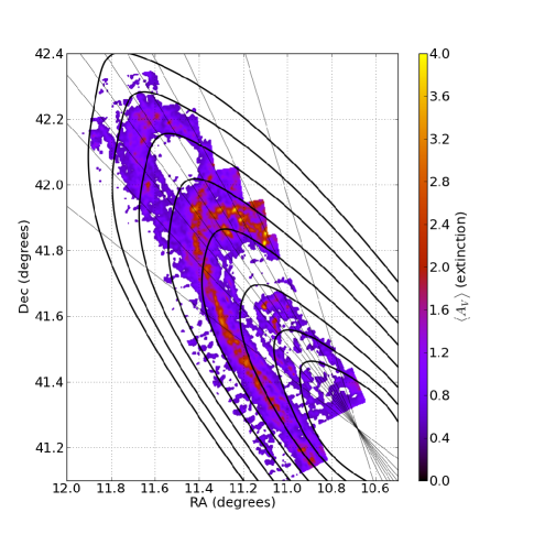
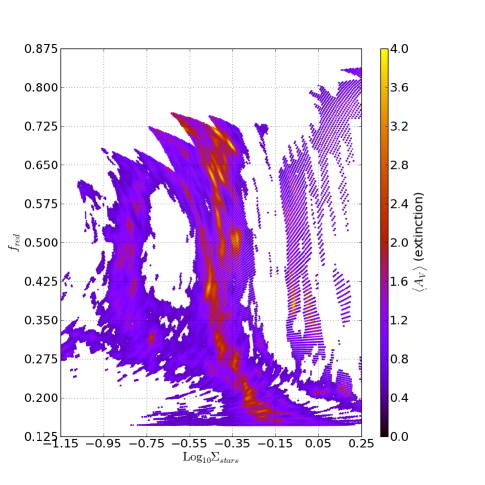
Figure 32.— Maps of the mean extinction $\langle A_{V}\rangle$ in terms of position on the sky (left), and transformed into coordinates tracking the local stellar surface density and the fraction of reddened stars (right); the latter quantity is a proxy for the range of radii that fall in a given line of sight. Only pixels with high extinction are plotted ($\langle A_{V}\rangle>0.5$). The heavy solid lines on the left panel show lines of constant $\log_{10}\Sigma_{stars}$, and the light diagonal lines indicate constant $f_{red}$ for the same coordinate grid used in the right panel.

In Figure 33 we plot the pixel-by-pixel correlations between the mean CMD-based extinction $\langle A_{V}\rangle$ (restricted to where $\langle A_{V}\rangle>0.5$) and the scale-corrected emission-based extinction $A_{V,emission}/2.53$. Each individual correlation sub-panel is calculated for pixels within one of the bins of $\log_{10}\Sigma_{stars}$ versus $f_{red}$ shown in the right panel of Figure 32. Thus, each sub-panel is equivalent to the upper right panel of Figure 28, but restricted to a subregion of the galaxy.

The correlations in Figure 33 can be used to look for large-scale spatially-dependent variations in the systematic bias and in the factor of 2.53 scale factor used to correct $A_{V,emission}$ to a better estimate of $A_{V}$. In each range of $\log_{10}\Sigma_{stars}$ and $f_{red}$, the diagonal line shows the expectation for a perfect 1:1 correlation. Data will fall along this line wherever $A_{V,emission}/2.53$ is a good estimator of $A_{V}$ and there are no systematic biases in either extinction measurement. If the scale factor is correct, but there is a systematic bias, then the data would have the same slope as the 1:1 line, but would be shifted horizontally or vertically.

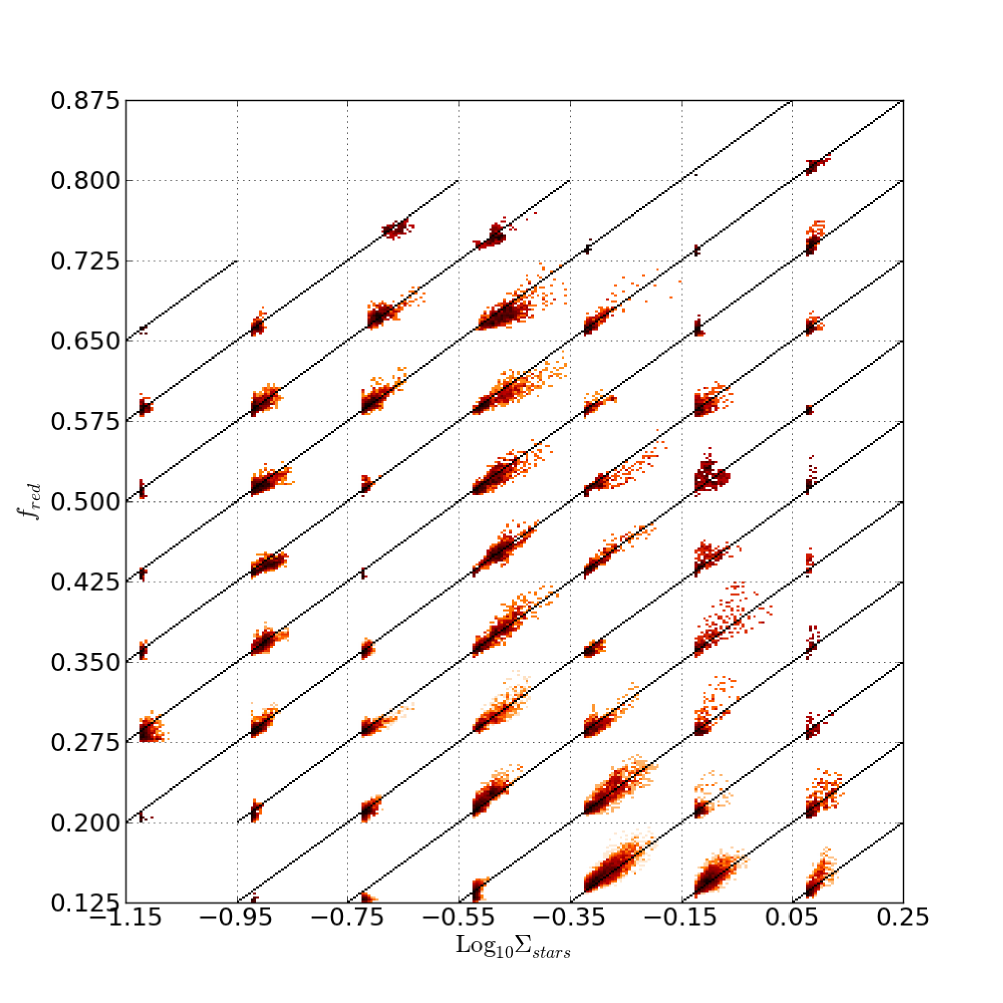
Figure 33.— Correlations between the CMD-based extinction and resolution-matched predictions for $A_{V}$ derived from emission (after correcting for $A_{V,emission}/\langle A_{V}\rangle=2.53$; see Sec. 6.2), calculated in bins of $\log_{10}\Sigma_{stars}$ and $f_{red}$, using the coordinate divisions shown in Figure 32. Each subpanel contains a plot equivalent to the upper right of Figure 28, with the CMD-based extinction on the horizontal axis and the emission-based extinction on the vertical axis. In each subpanel, $A_{V}$ is plotted between 0 and $4{\rm\,mag}$, and data with $A_{V,emission}<0.5{\rm\,mag}$ is not shown. Perfect correlations would fall along the diagonal lines. In every pixel, the correlations are strong. However, there are subtle differences in the slopes, depending on the specific values of $\log_{10}\Sigma_{stars}$ and $f_{red}$. These shifts are discussed in detail in Sec. 6.4.

6.4.1 Spatial Variations in $\langle A_{V}\rangle$ Correlations

In general, Figure 33 suggests that the CMD- and emission-based extinctions are well correlated throughout the galaxy, with no strong positional-dependent biases like those discussed in Sec. 4.2.5 & 5.3.2. There are two notable exceptions.

The first is seen at very high surface densities where the range of emission-based extinctions is much larger than the CMD-based extinctions. This difference is most probably due to the CMD-based extinction’s lack of sensitivity in the very inner disk, where the CMD is too broad to be sensitive to any but the highest extinctions (Figure 10). It may also be related to an inappropriate model for the unreddened CMD, due to the inner region’s complex stellar populations, which lead to large spatial variations in the fractions of M31’s disk, bulge, bar, and inner spheroid.

The second place where the correlation between the two extinction measures breaks down is at the very lowest surface densities. These regions are the origin of the small tail of stars with spuriously high CMD-based extinctions seen in Figure 28; most of these are in the region of bad photometry in Brick 22, or in the very outskirts of the disk where there are both few reddened stars and low extinctions, which leads to systematic errors (primarily due to systematic offsets in the photometry across the WFC3/IR chip) being more noticeable.

To quantify the trends in Figure 33, in Figure 34 we show the ratio $A_{V,emission}/\langle A_{V}\rangle$ at $\langle A_{V}\rangle=1$, as derived from fitting a linear function to the correlation in each subpanel of Figure 33 (i.e., as a function of $\log_{10}\Sigma_{stars}$ and $f_{red}$), after removing the factor of $\sim\!2.5$ correction to the Draine et al. (2014) extinctions. The plot has been scaled such that the overall ratio is in the middle of the color bar, and the range goes from zero to twice the observed ratio.

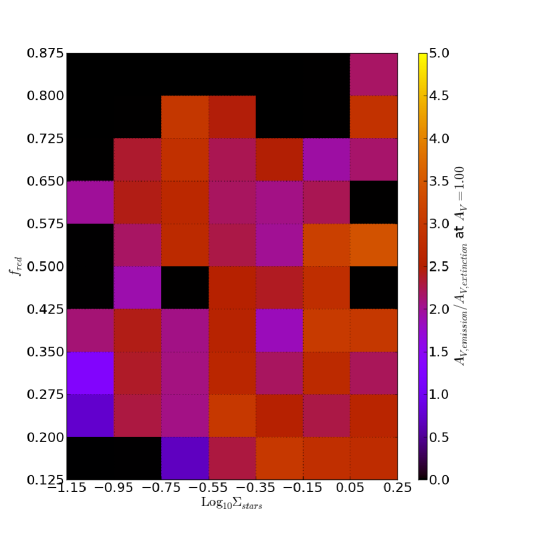
Figure 34.— Ratio between resolution-matched predictions for $A_{V}$ derived from emission (before correcting $A_{V,emission}$; see Sec. 6.2) and the CMD-based extinction, calculated in bins of $\log_{10}\Sigma_{stars}$ and $f_{red}$, using the coordinate divisions shown in Figure 32. The ratio is inferred at $\langle A_{V}\rangle=1$ from fitting the correlations shown in Figure 32, but without applying the factor of 2.53 correction to the dust-emission based extinctions; only bins whre the data extends to at least $\langle A_{V}\rangle=0.75$ are shown. The color bar spans from zero to twice the expected ratio. The spatial variations in the ratio are modest for the dust-emission estimates.

Figure 34 confirms our impressions from Figure 33, namely that the ratio of $A_{V}$’s is relatively uniform, except for the previously noted problems at very low surface densities.

6.5. Testing the Plank Collaboration et al. (2014) Exctinction Estimator

The Plank Collaboration et al. (2014) studies of reddening towards Milky Way molecular clouds and towards background QSOs strongly suggest that some of the spatial variation in $A_{V,emission}/\langle A_{V}\rangle$ that we see in Figures 30 & 33 may be correlated with a parameter related to the background radiation field. In the physical dust models of Draine & Li (2007), the dust is heated by a distribution of radiation field intensities, described by a $\delta$-function at the minimum intensity $U_{min}$ and a power-law distribution extending from $U_{min}$ to $U_{max}$ with slope $\alpha$. Plank Collaboration et al. (2014) argue that the dependence of the observed extinction on $U_{min}$ suggests that in practice $U_{min}$ is not solely tracing the minimum radiation field intensity, but instead is also compensating for variations in the properties of the underlying dust, some of which may be manifesting in departures from the spectral shape of the dust opacity expected in the Planck 857, 545, and 353 bands. Although these band are not used in the Draine et al. (2014) fits, the SPIRE 350$\mu$m and 500$\mu$m bands cover comparable wavelengths as the first two of these Planck bandpasses and both papers produce comparable dust mass estimates in M31 (Appendix A of Plank Collaboration et al., 2014). Thus, the Draine et al. (2014) fits are likely to be subject to the same effects.

Plank Collaboration et al. (2014) argue that $U_{min}$ can be used to make more accurate estimates of the expected extinction using the results of Draine & Li (2007) fitting. They propose an empirical linear formula to predict the extinction:

$$A_{V,emission,Planck}=(a\,U_{min}+b)\times A_{V,emission}$$ (16)

where $a=0.31$ and $b=0.35$ for the Milky Way’s diffuse gas and $a=0.33$ and $b=0.27$ for Milky Way molecular clouds. At a typical value of $U_{min}\!=\!0.5$, $A_{V,emission}/A_{V,emission,Planck}$ would have values of 2.0 and 2.3 for the diffuse ISM and molecular clouds, respectively. These values are comparable to the overall factor of 2.53 overestimate we derive here.

We can look for a similar linear dependence of $A_{V,emission}$ on $U_{min}$ within our data for M31. In Figure 35 we plot $U_{min}$ versus the percentange of the dust mass in PAHs from Draine et al. (2014), $q_{pah}$. Each pixel overlapping PHAT is color-coded by its measured value of $A_{V,emission}/\langle A_{V}\rangle$. We have excluded regions where $A_{V,emission}<0.5{\rm\,mag}$, to eliminate piexls where the emission and CMD-based extinctions will have the largest uncertainties.

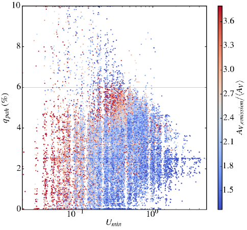
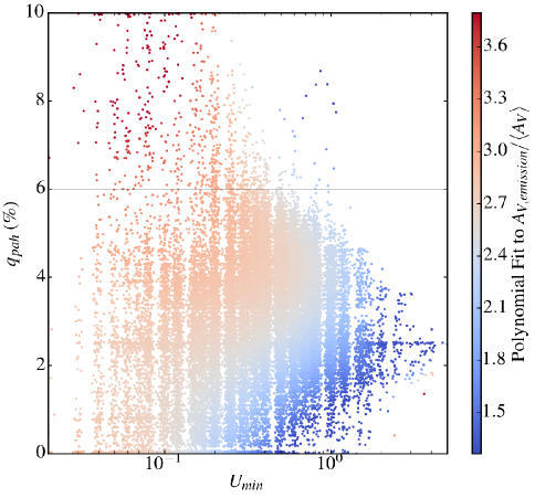
Figure 35.— The ratio between the emission-based extinction and the mean CMD-based extinction, as a function of $U_{min}$ and $q_{pah}$ derived in Draine et al. (2014). The left panel shows the data and the right panel shows the results of a 2nd order polynomial fit. The data show that the observed ratio depends on both $U_{min}$ and $q_{pah}$, not just on $U_{min}$ as was assumed in Plank Collaboration et al. (2014). The range of the color scale is chosen such that the grey value indicates the mean ratio of $A_{V,emission}/\langle A_{V}\rangle=2.53$ found in Sec. 6.2.1. The data is only plotted for points with $A_{V,emission}>0.5$, where uncertainties and biases in both methods are smaller. The fit was restricted to regions where $q_{pah}<6$%, because the regions with higher $q_{pah}$ are all found at the outer limits of where Draine et al. (2014) considers their fits to be reliable. For clarity, small random offsets have been added to both $U_{min}$ and $q_{pah}$ to compensate for the quantization of the original data and to better show the individual values of $A_{V,emission}/\langle A_{V}\rangle$.

Consistent with Plank Collaboration et al. (2014), the left panel of Figure 35 shows a tendency for $A_{V,emission}/\langle A_{V}\rangle$ to be overestimated where $U_{min}$ is low. However, the value of $A_{V,emission}/\langle A_{V}\rangle$ also appears to depend on $q_{pah}$ as well. The right panel of Figure 35 shows a 2nd order polynomial fit to the data with $q_{pah}<6$%; we exclude the highest values of $q_{pah}$ because they are all found in a region that is very close to the limit where Draine et al. (2014) consider their fits to no longer be robust to uncertainties in background subtraction. The resulting fit provides an alternate way to estimate the extinction from the Draine & Li (2007) dust models:

$$\begin{split}A_{V,emission}/\langle A_{V}\rangle=3.09-0.24q_{pah}+0.05q_{pah}^{2}\\ -4.77U_{min}-1.26U_{min}^{2}\\ +2.45U_{min}q_{pah}-0.34U_{min}q_{pah}^{2}\\ -1.26U_{min}^{2}q_{pah}+-0.18U_{min}^{2}q_{pah}^{2},\end{split}$$ (17)

where $q_{pah}$ is expressed as a percentage (rather than a fraction). We also provide a simpler first-order linear correction that produces an adequate fit to the data, but that leaves slightly larger systematic residuals:

$$\begin{split}A_{V,emission}/\langle A_{V}\rangle=2.57+0.08q_{pah}-1.24U_{min}\\ +0.17U_{min}q_{pah}.\end{split}$$ (18)

Figure 36 shows the result of applying either the Plank Collaboration et al. (2014) correction or the $U_{min}+q_{pah}$ correction from eqn. 17. Because our map of M31 includes both diffuse and molecular cloud components, for the Plank Collaboration et al. (2014) correction we adopt a slope and intercept midway between the two very similar linear corrections recommended for these two regimes ($a=0.32$, $b=0.31$).

The upper panels of Figures 36 show the observed ratio $A_{V,emission}/\langle A_{V}\rangle$ as a function of $U_{min}$, color-coded by either $q_{pah}$ (upper left) or the mean extinction ($\langle A_{V}\rangle$; upper right). The cyan stars show the median ratio in small bins of $U_{min}$, and the magnenta line shows the estimator derived in Plank Collaboration et al. (2014). The horizontal line is the overall 2.53 scaling we derived in Sec. 6.2.1 (i.e., Figure 28). The lower panels show the ratio that results after correcting the emission-based extinction by the 2nd-order polynomial fit from eqn. 17 (left panel) or the Plank Collaboration et al. (2014) correction (right panel).

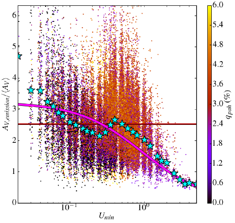
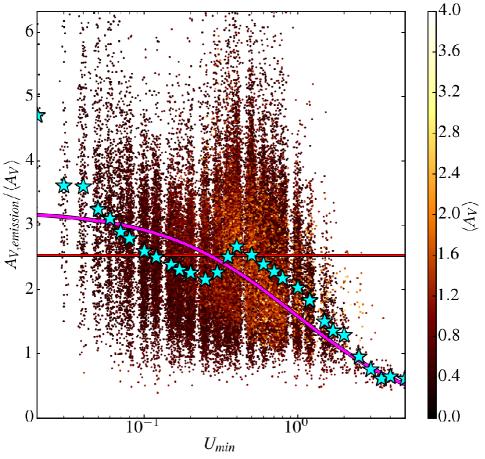
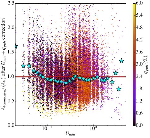
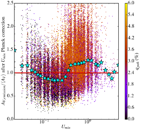
Figure 36.— The observed ratio between the emission-based extinction and the mean CMD-based extinction, as a function of $U_{min}$, color coded by $q_{pah}$ (top left, bottom row) or $\langle A_{V}\rangle$ (top right). Large cyan stars indicate the median value of $A_{V,emission}/\langle A_{V}\rangle$ in bins of $U_{min}$. In the top row, the solid magnenta line is the expectation based on the Plank Collaboration et al. (2014) correction, and the horizontal red line is the mean correction derived in Sec. 6.2.1. The bottom row shows the ratio after correcting $A_{V,emission}$ using the joint $U_{min}+q_{pah}$ correction shown in Figure 35 (left) and the Plank Collaboration et al. (2014) correction based on $U_{min}$ (right). The correction based on both $U_{min}$ and $q_{pah}$ shows much weaker systematic residuals, except at the very lowest values of $U_{min}$. The spatial correlation of the residuals is also reduced (see Figure 37). For clarity, small random offsets have been added to $U_{min}$ to compensate for the quantization of the original data and to better show the individual values of $A_{V,emission}/\langle A_{V}\rangle$.

Figure 36 shows that the Plank Collaboration et al. (2014) extinction estimator overall does a good job of correcting the extinction predicted by the Draine & Li (2007) models (lower right). The overall scale of the correction agrees very well, such that the ratio $A_{V,emission}/\langle A_{V}\rangle$ has a median within 25% of 1 after applying the $U_{min}$ correction to $A_{V,emission}$. However, when compared to the result of applying the $U_{min}+q_{pah}$ correction (lower left), the Plank Collaboration et al. (2014) correction leaves larger, systematic residuals. Both corrections leave significant scatter, however, which may be due to some of the effects discussed in Sec. 6.3.

In Figure 37 we compare the spatial distibution of $A_{V,emission}/\langle A_{V}\rangle$ after making the Plank Collaboration et al. (2014) correction (left) or the $U_{min}+q_{pah}$ correction from eqn. 17 (right). The left panel shows that the systematic residuals that the Plank Collaboration et al. (2014) correction leaves with $U_{min}$ produce large-scale spatially-correlated residuals in the predicted extinction map. With the Plank Collaboration et al. (2014) corrections, the extinction in the inner galaxy and half of the major star forming ring is overestimated, and the extinction in the outer galaxy is underestimated. When compared to Figure 30, the Plank Collaboration et al. (2014) correction appears to produce larger, more spatially-correlated residuals than applying a single $\sim$2.5 correction factor.

In contrast, the $U_{min}+q_{pah}$ correction from eqn. 17 produces a map that appears to be free from the large scale systematics that were visible in Figures 30 & 33. The only noticeable exceptions are the two regions of high star formation intensity discussed in Sec. 6.3 (see Figure 31) where the corrected value of $A_{V,emission}$ is too low, and a region near the end of M31’s long bar in the inner disk, where the corrected value of $A_{V,emission}$ is too high. This latter mismatch may be due to an error in $\langle A_{V}\rangle$ associated with rapidly changing stellar poplations at this position. Other than these regions, and the expected convergence of the uncorrected value of $A_{V,emission}$ and $\langle A_{V}\rangle$ in regions where $A_{V}\rightarrow 0$ in the outermost disk, the corrected map looks quite uniform. This suggests that our earlier suspicion (Sec. 6.3) that some of the observed systematic variations were tracing the variation in $q_{pah}$ was correct.

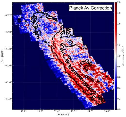
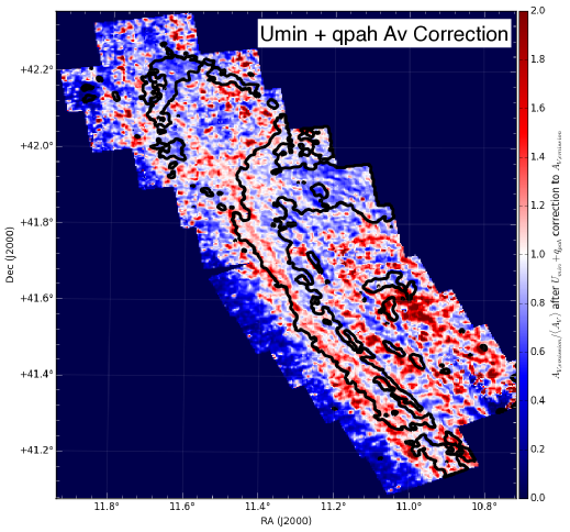
Figure 37.— Maps of the ratio between the emission-based extinction and the mean CMD-based extinction, after correcting $A_{V,emssion}$ by applying either the Plank Collaboration et al. (2014) correction that uses only $U_{min}$ (left) or a polynomial correction based on both $U_{min}$ and $q_{pah}$ (right). The (Plank Collaboration et al., 2014) correction does a good job of correcting the overall normalization, but introduces a clear radial bias and does not correct some of the largest, spatially-coherent features in the map. The correction based on both $U_{min}$ and $q_{pah}$ produces a much more uniform map. The notable discrepancies are in the inner disk where $\langle A_{V}\rangle$ values are known to be more uncertain, and in the two most actively starforming complexes identified in Figure 31.

6.5.1 Interpreting the Dependence on $q_{pah}$

As Plank Collaboration et al. (2014) noted, the dependence of $A_{V,emission}/\langle A_{V}\rangle$ on other parameters of the Draine & Li (2007) fits does not necessarily suggest that the true values of those parameters are actually changing. Any fitting procedure will tend to produce correlated residuals in the values of parameters when the underlying model is not perfect. The mass contained in PAHs is quite small (typically less than 5%), and they are responsible for very little of the extinction in the NIR. Thus, the fact that we see a correlation between the $A_{V,emission}/\langle A_{V}\rangle$ and $q_{pah}$ is unlikely to indicate that variations in the PAH fraction are actually causing variations in the extinction. Instead, it is likely that both $U_{min}$ and $q_{pah}$ are compensating for subtle differences in the spectral shape of the dust’s opacity and emissivity, and for complexities in how the interstellar radiation field relates to dust emission.

One interesting feature in Figure 36 points to possible connections to the role of dust heating and to the differences between dust in the diffuse ISM and in star forming regions. The upper panels of Figure 36 appear to show two broad diagonal sequences that have a similar variation of $A_{V,emission}/\langle A_{V}\rangle$ with $U_{min}$, but that are shifted horizontally from each other. At low values of $U_{min}<0.2$, the majority of points have low PAH fractions and low extinctions. At higher values of $U_{min}>0.2$, the sequence is dominated by regions with higher PAH fractions and higher extinctions. This bifurcation may reflect that the appropriate conversion between emission and extinction largely separates into two different regimes – one associated with the diffuse ISM and one associated with higher star formation rate intensities and larger typical gas columns. Although the Draine & Li (2007) models attempt to include this effect by allowing some fraction of the dust to be heated by harder radiation fields associated with photo-dissociation regions (PDRs), it is unlikely that a single physical dust model can fully capture the complexity of dust heating and composition that is found in a typical PDR.

In light of this, although Figures 35–37 show that the correction to $A_{V,emission}$ given in eqn. 17 does an excellent job of predicting the extinction in M31, the correction should not necessarily be expected to do an equally good job in other circumstances. The joint distribution of $U_{min}$ and $q_{pah}$ is likely to reflect the dust heating and composition that is particular to M31, to first order. The second order dependence of $A_{V,emission}/\langle A_{V}\rangle$ on $U_{min}$ and $q_{pah}$ seems likely to arise from deviations between the assumptions of the Draine & Li (2007) physical dust model and the real behavior of M31’s dusty ISM. Neither of these situations will necessarily be reproduced in galaxies with very different star formation rates, metallicities, or dense gas fractions. Likewise, if the variation of $A_{V,emission}/\langle A_{V}\rangle$ with $U_{min}$ and $q_{pah}$ is due to the fit compensating for subtle mismatches in the underlying dust model, then fits that use data taken in different bandpasses and/or with different physical resolutions may not compensate for these effects in exactly the same way. As a result, we do not expect that the correction in eqn. 17 will be one that holds generically in all situations. The overall scaling of a factor of $\sim\!2-2.5$ seems robust, given that comparable corrections were needed both in M31 and in the diffuse and the molecular components of the Milky Way (Plank Collaboration et al., 2014), but the exact second-order dependence of $A_{V,emission}/\langle A_{V}\rangle$ on $U_{min}$ and $q_{pah}$ may be variable.

7. Conclusions

In this paper we have developed a new method for mapping extinction in external galaxies. The method is based on using NIR observations of RGB stars. These stars have a very narrow distribution in NIR color as a function of magnitude, allowing one to diagnose extinction as a redward shift in the position of the RGB on a CMD. We model the NIR CMD as a combination of a foreground of unreddened stars, and a background of stars that lie behind a thin layer of dust. The background stars sample the distribution of extinctions within the dust layer, which we characterize with a single log-normal function. We fit for the fraction of stars behind the dust layer, and the characteristic parameters of the log-normal (median extinction, dimensionless width), from which we derive the mean and dispersion of the distribution of $A_{V}$. We carry out this analysis using stars from the PHAT survey of M31, selected in $25{\rm\,pc}$ ($6.6\arcsec$) bins with $12.5{\rm\,pc}$ sampling.

The resulting map is the highest resolution tracer of extinction available in M31 to date. More importantly, it offers a completely independent assessment of the properties of the cold ISM, allowing it to be compared with other widely-used tracers, including emission from dust and from cool gas (Hi and CO).

Our maps reveal a factor of $\sim$2.5 offset between the extinction directly measured from RGB stars and the extinction inferred from recent maps of the dust emission (e.g., Draine et al., 2014). This difference is unlikely to be due to the NIR CMD fitting, and instead suggests that there is significantly more emission associated with a given amount of dust extinction than expected for the most recent calibration of the Draine & Li (2007) models. Given how important these models have become to the study of external galaxies, understanding the origin of this offset is vital. Similar offsets have been seen in the Milky Way (Plank Collaboration et al., 2014), where they were found to have a second order dependence on the Draine & Li (2007) estimates of the strength of the background radiation field. We show that the offset in M31 depends on the measured percentage of PAH’s as well. We provide a fitting formula to allow the extinction to be estimated from the results of fitting to the Draine & Li (2007) models.

Given the success of this technique, it is natural to think of possible extensions. Within M31, one might consider including optical data in the analysis to provide better sensitivity at low extinction. However, unlike the NIR, the color of the optical RGB is quite sensitive to age, leading to a much broader RGB for galaxies with extended star formation histories, and greater sensitivity to stellar population gradients. Given that the efficacy of the technique depends on having sufficient reddening to move stars out of the unreddened CMD, it is not immediately clear that optical data’s greater sensitivity to reddening would counteract the problem of an intrinsically broader RGB. We address these issues more quantitatively in an appendix (Sec. A).

Some of the difficulty in incorporating optical and UV data into an RGB-only analysis can be sidestepped by carrying out joint UV$+$optical$+$NIR fitting of every star’s spectral energy distribution (Gordon et al 2015, submitted). This approach was very successful in Zaritsky et al. (2002) and Zaritsky et al. (2004)’s analyses of the Magellanic Clouds, but used UV and optical data alone, as was appropriate for the much lower extinctions in these galaxies. Fitting PHAT’s 6-filter photometry should offer an excellent opportunity to probe down to lower extinctions and to assess the detailed connections between dust and different ages of stellar populations, although with more dependence on the accuracy of the underlying stellar models.

As another possible extension, one might also think of applying this technique to other galaxies, with M33 being an obvious target. In more distant galaxies, however, the apparent width of the RGB will be a limiting factor when using current facilities; more distant galaxies have higher levels of crowding that limit the photometric accuracy possible with a given telescope+camera (e.g. Olsen et al., 2003), leading to a wider RGB. However, a next generation telescope (either 30m class from the ground, or an 10-12m in space) with a high resolution NIR camera would make this technique viable throughout the local volume.

Appendix A Applying This Technique at Other Wavelengths

Although we have developed and applied this technique in the NIR, it is natural to consider whether it might also be useful in other wavelength regimes. In particular, by incorporating optical data we could potentially improve our sensitivity to low extinctions, because of the greater impact of reddening and extinction at bluer wavelengths. As we now show, the increased sensitivity to reddening comes at a cost, because the underlying CMD is far more sensitive to population effects in bluer filter.

The key issues that affect the sensitivity of our technique are: (1) the amount of reddening produced by a given $A_{V}$; (2) the amount of reddening needed to move a star clearly out of the RGB; (3) the spatial uniformity of the unreddened RGB; (4) the maximum $A_{V}$ that can be detected before losing a star below the photometric limit; and (5) the total number of well-measured stars on the RGB. Incorporating data from bluer wavelengths improves the first issue, but its effect on the remaining issues is unclear.

To assess the impact of these issues outside the NIR, we construct CMDs of the unreddened RGB in a variety of filter combinations. In Figure 38 we show Hess diagrams constructed within Brick 12, Field 7, which has extremely low reddening as judged from both the NIR CMD and the Draine et al. (2014) maps. To allow us to compare arbitrary filter combinations, we use the simultaneous six filter *.gst photometry described in Williams et al (2014), which supersedes the first generation photometry in Dalcanton et al. (2012); these photometry have not had cuts applied to optimize rejection of spurious measurements redward of the RGB, but are sufficient for our purposes here. The horizontal purple bars indicate the median photometric uncertainty at 5 different magnitudes; the uncertainties are a quadrature sum of the photon counting uncertainties reported by DOLPHOT and a flat $0.015{\rm\,mag}$ uncertainty due to calibration (Dalcanton et al., 2012). The diagonal red line shows the effect of $\Delta A_{V}=2{\rm\,mag}$, using $A_{F475W}/A_{V}=1.1591$ and $A_{F814W}/A_{V}=0.5962$, which we derived analogously to $A_{F110W}/A_{V}$ and $A_{F160W}/A_{V}$ above in Sec. 3.

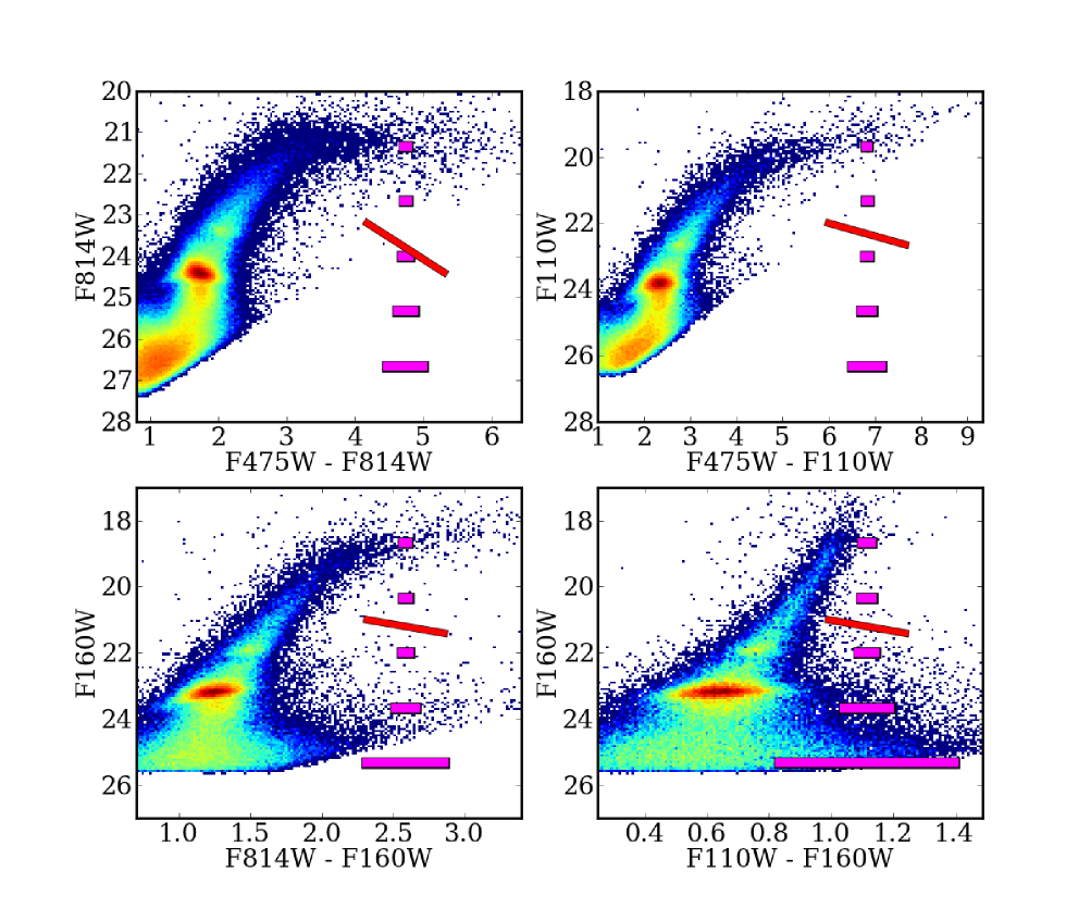
Figure 38.— Comparing the sensitivity of different filter combinations to reddening and extinction. Plots show logarithmically-scaled Hess diagrams of the RGB region in 4 different filter combinations, for one of the lowest reddening regions of the PHAT survey (Brick 12, Field 1, plotting the ‘‘gst’’ photometry). The horizontal magenta bars indicate the median reported photometric uncertainty at the plotted magnitude, including an additional systematic component of $\sigma_{color}=0.015$ (see Dalcanton et al., 2012); these bars do not include errors due to crowding, which will increase significantly near the limiting magnitude of the data. In general, the width of the RGB is significantly larger than the photometric uncertainties, indicating that variations in the age and metallicity of the stellar population is primarily responsible for broadening the RGB. This effect is worse in the optical filters, but negligible in the NIR, where the RGB is intrinsically narrow and has a width almost entirely dominated by photometric uncertainties. The red bar shows the shift in color and magnitude that would be caused by $\Delta A_{V}=2$ magnitudes of extinction; and the range of plotted colors is adjusted so that it covers the amount of reddening caused by a constant $\Delta A_{V}=10$ magnitudes of extinction. The intrinsic width of the RGB in terms of $\Delta A_{V}$ is much broader in the optical filters than the NIR, which cancels out any possible benefit which may have resulted from the optical’s greater sensitivity to extinction, compared to the NIR.

The first, and most important, figure of merit needed to interpret Figure 38 is the relative width of the RGB compared to the length of the reddening vector. If the RGB is narrow compared to the reddening vector, then even modest $A_{V}$ will move a star clearly off the unreddened sequence, increasing the sensitivity to low dust columns. We facilitate this comparison by plotting each CMD with a color range that corresponds to a constant $\Delta A_{V}$, such that the reddening vector has the same width in each panel. With this display choice, CMDs that appear wider are indeed “wider compared to a given $\Delta A_{V}$”.

Inspection of Figure 38 shows that the RGB is intrinsically narrower in the NIR than in any other filter combination. In other words, although the reddening in $F110W-F160W$ is smallest for a given $A_{V}$, our ability to actually detect that reddening is largest. In terms of $A_{V}$, the NIR RGB has a width of $\Delta A_{V}=0.38{\rm\,mag}$ for stars with $19.5<F160W<20.5$, whereas the optical CMD (upper left) has $\Delta A_{V}=0.54{\rm\,mag}$.

The narrowness of the NIR CMD comes in large part because of the cancellation of age and metallicity in RGB isochrones. Older stars tends to have redder RGBs, but these stars also tend to have lower metallicities, which drives their colors back blueward. In the NIR, these effects are intrinsically small, and also largely cancel out. In contrast, in the optical these effects are much larger and do not effectively cancel out. This unfortunate fact leads to broader CMDs in the optical. Moreover, it points to increased sensitivity of the optical CMD to variations in the underlying stellar population’s age and/or metallicity. While this is good for stellar population studies, it means that one expects much larger spatial gradients in the properties of the unreddened RGB, making the construction of an accurate, smoothly varying “unreddened” CMD far more difficult. Thus, by the criteria listed above, issues (2) and (3) are negatively affected by including bluer filters.

Issue (4) is also further compromised when moving to bluer filters. Inspection of the optical CMDs in the top row shows that the blue magnitude limit in $F475W$ cuts off stars with more than $A_{V}\sim 2$. In contrast, the redder CMDs in the bottom row allow a much larger range of $A_{V}$ to be detected, giving better constraints on the median $A_{V}$ and the shape of the reddening distribution. This limitation can not necessarily be overcome by a larger investment of telescope time, given that the data is already crowding limited.

The one area where switching to optical filter may improve sensitivity is in the number of stars (i.e., issue #5). Comparing photometric errors (magenta bars) to the width of the RGB shows that bluer filters can accurately track the RGB down to fainter CMD features, increasing the number of stars that can be used in a given area. This difference potentially allows one to increase the resolution of the extinction maps. However, the higher stellar density would have only modest effects in high extinction regions, since most of the newly detected stars are close to the magnitude limit.

Rather than switching entirely to the optical, it may be that some gains could be achieved by using $F814W-F160W$ to measure the reddening. The RGB is less than 5% wider than in the NIR (in terms of $\Delta A_{V}$), so the sensitivity to small extinctions should be comparable. However, the photometric errors are proportionally smaller, due to the wider color baseline and the better accuracy in $F814W$ compared to F110W. These improved errors should allow us to use stars further down the RGB, which increases the spatial density of stars. One can then use smaller analysis pixels to increase the spatial resolution of the extinction map. Unlike in the optical, these additional stars are comfortably above the magnitude limit, even for significant reddening, and thus they should provide useful leverage on the distribution of reddenings. It is not clear, however, whether these gains trump the likely increase in the susceptibility of the RGB structure to age and metallicity variations.

Appendix B Smooth Models for the Dust Distribution

During the course of this work, we also considered a model where the reddening seen in the CMD was produced by a smooth layer of dust embedded within the stellar disk. As we show here, this assumption produces distributions of extinction that are inconsistent with the data, leading to the need for the alternative “thin screen with a log-normal distribution of extinction” model adopted in this paper.

We calculate the expected distribution of stellar extinctions for a smooth dust model as follows. We assume that the dust is embedded within a stellar disk with a scale height $z_{\star}$. We model the stellar disk using the probability $p_{\star}(z;z_{\star})$ that a star is found at height $z$ relative to the midplane of the stellar disk (assuming that positive values of $z$ correspond to stars that are closer to us than the midplane at $z=0$). The stellar density distribution can be assumed to be a Gaussian, an exponential, or any other reasonable functional form.

We first assume that the dust is smoothly distributed within a vertical distribution $p_{d}(z;z_{d},z_{0})$ with scale height $z_{d}$, centered at a height $z_{0}$ relative to the midplane of the stellar disk. We assume that the total extinction of the integrated dust column is $A_{V,tot}$. The integrated extinction seen for a star at height $z$ is then

$$A_{V}(z)=A_{V,tot}\,\int^{\infty}_{z}{p_{d}(z;z_{d},z_{0})\,dz}.$$ (B1)

If we assume that the vertical distribution of dust is an exponential and let $z^{\prime}\equiv z-z_{0}$, then

$$A_{V}(z=z^{\prime}+z_{0})=\frac{A_{V,tot}}{2}\,\left[\frac{|z^{\prime}|-z^{\prime}}{|z^{\prime}|}+\frac{z^{\prime}}{|z^{\prime}|}\,e^{-|z^{\prime}|/z_{d}}\right]$$ (B2)

The probability $p_{A}(A_{V})\,dA_{V}$ of finding a star with an extinction between $A_{V}$ and $A_{V}+dA_{V}$ is then

$$p_{A}(A_{V})\,dA_{V} = p_{\star}(z(A_{V});z_{\star})\,\left|\frac{dz}{dA_{V}}\right|\,dA_{V}$$ (B3)

$$= p_{\star}(z(A_{V});z_{\star})\,\left(\frac{z_{d}}{A_{V,tot}/2}\right)\,\frac{1}{\frac{z^{\prime}}{|z^{\prime}|}\,\frac{A_{V}}{A_{V,tot}/2}-\frac{|z^{\prime}|-z^{\prime}}{|z^{\prime}|}}\,dA_{V}$$ (B4)

where $z^{\prime}\equiv z(A_{V})-z_{0}$ and $z(A_{V})$ is the inverse of equation B2:

$$z(A_{V})=z_{0}-z_{d}\,\frac{\Delta A_{V}}{|\Delta A_{V}|}\,\ln{\left(\frac{|\Delta A_{V}|-\Delta A_{V}}{|\Delta A_{V}|}+\frac{\Delta A_{V}}{|\Delta A_{V}|}\,\left(\frac{A_{V}}{A_{V,tot}/2}\right)\right)},$$ (B5)

assuming $\Delta A_{V}\equiv A_{V,tot}/2-A_{V}$.

The resulting distribution of $p_{A}(A_{V})$ is shown in Figure 39 for the case of a Gaussian distribution of stars. When the scale height of the dust is less than that of the stars, the probability distribution has two strong peaks — one at $A_{V}=0$, corresponding to unreddened stars seen on the near side of the dust layer, and one at $A_{V}=A_{V,tot}$, corresponding to stars seen on the far side of the dust layer, after they have experienced the entire dust column. The relative height of the two peaks depends on the position of the dust layer relative to the stars, with the unreddened peak becoming stronger when the dust layer is on the far side of the stellar midplane. As the scale height of the dust increases, there are fewer stars with either zero reddening or the maximum reddening (i.e., all stars are embedded within the dust), and the two peaks move together towards a typical extinction of half the total integrated extinction.

Figure 39.— Probability distributions for a smooth exponential dust layer with scale height $z_{dust}$ embedded within a Gaussian stellar disk of scale height $z_{stars}$, for different ratios between the scale heights of the dust and stars. When the dust layer is thin compared to the stars, the stars have a bimodal distribution of $A_{V}$, falling in an either unreddened or reddened peak. This bimodality becomes less distinct as the thickness of the dust and stars become comparable. The left hand panel shows a dust layer centered at the stellar midplane and the right hand panel shows a dust layer that is shifted to the far side of the stellar midplane by one half the scale height of the stars. When the dust lies on the far side of the midplane, a larger fraction of stars have low extinctions.

To transfer $p_{A}(A_{V})$ to the observed reddening distribution for the RGB, one must convolve equation B3 with the intrinsic distribution of RGB colors along the reddening vector. For an intrinsic Gaussian distribution of RGB colors and a thin dust layer, one would then expect to see two skewed Gaussian peaks – an unreddened Gaussian skewed towards redder colors, and a highly reddened Gaussian skewed toward bluer colors – provided that the expected total reddening from dust is significantly larger than the intrinsic width of the RGB colors. The reddened and unreddened Gaussians should have identical widths when the dust is centered on the midplane, but can have somewhat different widths if the dust lane is not aligned with the stars (right hand panel of Figure 39), in the sense that the peak containing a higher fraction of stars should also be wider. However, there are many regions in our data which appear to violate this condition. Frequently the reddened distribution is nearly an order of magnitude broader than the unreddened peak, which cannot be accounted for in models with a smooth dust layer. We therefore reject a smooth dust layer as being an appropriate model for these observations.

References

- Abreu-Vicente et al. (2015) Abreu-Vicente, J., Kainulainen, J., Stutz, A., Henning, T., & Beuther, H. 2015, ArXiv e-prints, arXiv:1507.00538
- Alton et al. (2004) Alton, P. B., Xilouris, E. M., Misiriotis, A., Dasyra, K. M., & Dumke, M. 2004, A&A, 425, 109
- Alves et al. (1998) Alves, J., Lada, C. J., Lada, E. A., Kenyon, S. J., & Phelps, R. 1998, ApJ, 506, 292
- Alves et al. (2014) Alves, J., Lombardi, M., & Lada, C. J. 2014, A&A, 565, A18
- Alves et al. (2001) Alves, J. F., Lada, C. J., & Lada, E. A. 2001, Nature, 409, 159
- Alves de Oliveira et al. (2014) Alves de Oliveira, C., Schneider, N., Merín, B., et al. 2014, A&A, 568, A98
- Aniano et al. (2012) Aniano, G., Draine, B. T., Calzetti, D., et al. 2012, ApJ, 756, 138
- Arce & Goodman (1999) Arce, H. G., & Goodman, A. A. 1999, ApJ, 517, 264
- Astropy Collaboration et al. (2013) Astropy Collaboration, Robitaille, T. P., Tollerud, E. J., et al. 2013, A&A, 558, A33
- Ballesteros-Paredes et al. (2012) Ballesteros-Paredes, J., D’Alessio, P., & Hartmann, L. 2012, MNRAS, 427, 2562
- Ballesteros-Paredes et al. (2011) Ballesteros-Paredes, J., Vázquez-Semadeni, E., Gazol, A., et al. 2011, MNRAS, 416, 1436
- Barmby et al. (2006) Barmby, P., Ashby, M. L. N., Bianchi, L., et al. 2006, ApJ, 650, L45
- Beaton et al. (2007) Beaton, R. L., Majewski, S. R., Guhathakurta, P., et al. 2007, ApJ, 658, L91
- Beaumont et al. (2012) Beaumont, C. N., Goodman, A. A., Alves, J. F., et al. 2012, MNRAS, 423, 2579
- Bendo et al. (2012) Bendo, G. J., Boselli, A., Dariush, A., et al. 2012, MNRAS, 419, 1833
- Bergin & Tafalla (2007) Bergin, E. A., & Tafalla, M. 2007, ARA&A, 45, 339
- Berkhuijsen & Fletcher (2008) Berkhuijsen, E. M., & Fletcher, A. 2008, MNRAS, 390, L19
- Bianchi (2008) Bianchi, S. 2008, A&A, 490, 461
- Boissier et al. (2004) Boissier, S., Boselli, A., Buat, V., Donas, J., & Milliard, B. 2004, A&A, 424, 465
- Boselli et al. (2010) Boselli, A., Eales, S., Cortese, L., et al. 2010, PASP, 122, 261
- Braun et al. (2009) Braun, R., Thilker, D. A., Walterbos, R. A. M., & Corbelli, E. 2009, ApJ, 695, 937
- Brinks & Bajaja (1986) Brinks, E., & Bajaja, E. 1986, A&A, 169, 14
- Brunt (2015) Brunt, C. M. 2015, MNRAS, 449, 4465
- Butler & Tan (2009) Butler, M. J., & Tan, J. C. 2009, ApJ, 696, 484
- Butler & Tan (2012) —. 2012, ApJ, 754, 5
- Cambrésy (1999) Cambrésy, L. 1999, A&A, 345, 965
- Cambrésy et al. (2002) Cambrésy, L., Beichman, C. A., Jarrett, T. H., & Cutri, R. M. 2002, AJ, 123, 2559
- Cambrésy et al. (1997) Cambrésy, L., Epchtein, N., Copet, E., et al. 1997, A&A, 324, L5
- Cardelli et al. (1989) Cardelli, J. A., Clayton, G. C., & Mathis, J. S. 1989, ApJ, 345, 245
- Cernicharo & Bachiller (1984) Cernicharo, J., & Bachiller, R. 1984, A&AS, 58, 327
- Chakrabarti et al. (2003) Chakrabarti, S., Laughlin, G., & Shu, F. H. 2003, ApJ, 596, 220
- Chemin et al. (2009) Chemin, L., Carignan, C., & Foster, T. 2009, ApJ, 705, 1395
- Ciardi et al. (1998) Ciardi, D. R., Woodward, C. E., Clemens, D. P., Harker, D. E., & Rudy, R. J. 1998, AJ, 116, 349
- Combes (1991) Combes, F. 1991, ARA&A, 29, 195
- Compiègne et al. (2010) Compiègne, M., Flagey, N., Noriega-Crespo, A., et al. 2010, ApJ, 724, L44
- Compiègne et al. (2011) Compiègne, M., Verstraete, L., Jones, A., et al. 2011, A&A, 525, A103
- Dalcanton et al. (2012) Dalcanton, J. J., Williams, B. F., Lang, D., et al. 2012, ApJS, 200, 18
- Dale et al. (2012) Dale, D. A., Aniano, G., Engelbracht, C. W., et al. 2012, ApJ, 745, 95
- Dasyra et al. (2005) Dasyra, K. M., Xilouris, E. M., Misiriotis, A., & Kylafis, N. D. 2005, A&A, 437, 447
- Desert et al. (1990) Desert, F.-X., Boulanger, F., & Puget, J. L. 1990, A&A, 237, 215
- Devereux et al. (1994) Devereux, N. A., Price, R., Wells, L. A., & Duric, N. 1994, AJ, 108, 1667
- Dickman (1978) Dickman, R. L. 1978, AJ, 83, 363
- Disney et al. (1989) Disney, M., Davies, J., & Phillipps, S. 1989, MNRAS, 239, 939
- Dobashi (2011) Dobashi, K. 2011, PASJ, 63, 1
- Dobashi et al. (2008) Dobashi, K., Bernard, J.-P., Hughes, A., et al. 2008, A&A, 484, 205
- Dobashi et al. (2009) Dobashi, K., Bernard, J.-P., Kawamura, A., et al. 2009, AJ, 137, 5099
- Dobashi et al. (2005) Dobashi, K., Uehara, H., Kandori, R., et al. 2005, PASJ, 57, 1
- Dobbs & Bonnell (2006) Dobbs, C. L., & Bonnell, I. A. 2006, MNRAS, 367, 873
- Dolphin (2000) Dolphin, A. E. 2000, PASP, 112, 1383
- Dong et al. (2014) Dong, H., Li, Z., Wang, Q. D., et al. 2014, ApJ, 785, 136
- Dorman et al. (2015) Dorman, C. E., Guhathakurta, P., Seth, A. C., et al. 2015, ApJ, 803, 24
- Draine (2003) Draine, B. T. 2003, ARA&A, 41, 241
- Draine & Li (2007) Draine, B. T., & Li, A. 2007, ApJ, 657, 810
- Draine et al. (2014) Draine, B. T., Aniano, G., Krause, O., et al. 2014, ApJ, 780, 172
- Driver et al. (2007) Driver, S. P., Allen, P. D., Liske, J., & Graham, A. W. 2007, ApJ, 657, L85
- Dunne et al. (2011) Dunne, L., Gomez, H. L., da Cunha, E., et al. 2011, MNRAS, 417, 1510
- Elmegreen (1980) Elmegreen, D. M. 1980, ApJ, 242, 528
- Federrath et al. (2010) Federrath, C., Roman-Duval, J., Klessen, R. S., Schmidt, W., & Mac Low, M.-M. 2010, A&A, 512, A81
- Ford et al. (2013) Ford, G. P., Gear, W. K., Smith, M. W. L., et al. 2013, ApJ, 769, 55
- Foreman-Mackey et al. (2013) Foreman-Mackey, D., Hogg, D. W., Lang, D., & Goodman, J. 2013, PASP, 125, 306
- Frerking et al. (1982) Frerking, M. A., Langer, W. D., & Wilson, R. W. 1982, ApJ, 262, 590
- Frieswijk & Shipman (2010) Frieswijk, W. W. F., & Shipman, R. F. 2010, A&A, 515, A51
- Fritz et al. (2012) Fritz, J., Gentile, G., Smith, M. W. L., et al. 2012, A&A, 546, A34
- Froebrich & del Burgo (2006) Froebrich, D., & del Burgo, C. 2006, MNRAS, 369, 1901
- Froebrich et al. (2007) Froebrich, D., Murphy, G. C., Smith, M. D., Walsh, J., & Del Burgo, C. 2007, MNRAS, 378, 1447
- Froebrich & Rowles (2010) Froebrich, D., & Rowles, J. 2010, MNRAS, 406, 1350
- Galametz et al. (2011) Galametz, M., Madden, S. C., Galliano, F., et al. 2011, A&A, 532, A56
- Galametz et al. (2012) Galametz, M., Kennicutt, R. C., Albrecht, M., et al. 2012, MNRAS, 425, 763
- Galliano et al. (2011) Galliano, F., Hony, S., Bernard, J.-P., et al. 2011, A&A, 536, A88
- Girardi et al. (2008) Girardi, L., Dalcanton, J., Williams, B., et al. 2008, PASP, 120, 583
- Gonzalez et al. (2011) Gonzalez, O. A., Rejkuba, M., Zoccali, M., Valenti, E., & Minniti, D. 2011, A&A, 534, A3
- Gonzalez et al. (2012) Gonzalez, O. A., Rejkuba, M., Zoccali, M., et al. 2012, A&A, 543, A13
- Goodman et al. (2009) Goodman, A. A., Pineda, J. E., & Schnee, S. L. 2009, ApJ, 692, 91
- Goodman & Weare (2010) Goodman, J., & Weare, J. 2010, Comm. App. Math. Comp. Sci., 5, 6+
- Gordon et al. (2003) Gordon, K. D., Clayton, G. C., Misselt, K. A., Landolt, A. U., & Wolff, M. J. 2003, ApJ, 594, 279
- Gordon et al. (2006) Gordon, K. D., Bailin, J., Engelbracht, C. W., et al. 2006, ApJ, 638, L87
- Green et al. (2015) Green, G. M., Schlafly, E. F., Finkbeiner, D. P., et al. 2015, ArXiv e-prints, arXiv:1507.01005
- Gregersen et al. (2015) Gregersen, D., Seth, A. C., Williams, B. F., et al. 2015, submitted to ApJ
- Groves et al. (2012) Groves, B., Krause, O., Sandstrom, K., et al. 2012, MNRAS, 426, 892
- Harjunpää et al. (2004) Harjunpää, P., Lehtinen, K., & Haikala, L. K. 2004, A&A, 421, 1087
- Harris et al. (1997) Harris, J., Zaritsky, D., & Thompson, I. 1997, AJ, 114, 1933
- Hayakawa et al. (2001) Hayakawa, T., Cambrésy, L., Onishi, T., Mizuno, A., & Fukui, Y. 2001, PASJ, 53, 1109
- Hennebelle & Falgarone (2012) Hennebelle, P., & Falgarone, E. 2012, A&A Rev., 20, 55
- Hill et al. (2008) Hill, A. S., Benjamin, R. A., Kowal, G., et al. 2008, ApJ, 686, 363
- Hopkins (2013) Hopkins, P. F. 2013, MNRAS, 430, 1880
- Hunter (2007) Hunter, J. D. 2007, Computing in Science & Engineering, 9, 90
- Innanen et al. (1982) Innanen, K. A., Kamper, K. W., van den Bergh, S., & Papp, K. A. 1982, ApJ, 254, 515
- Jurić et al. (2008) Jurić, M., Ivezić, Ž., Brooks, A., et al. 2008, ApJ, 673, 864
- Kainulainen et al. (2011a) Kainulainen, J., Alves, J., Beuther, H., Henning, T., & Schuller, F. 2011a, A&A, 536, A48
- Kainulainen et al. (2011b) Kainulainen, J., Beuther, H., Banerjee, R., Federrath, C., & Henning, T. 2011b, A&A, 530, A64
- Kainulainen et al. (2009) Kainulainen, J., Beuther, H., Henning, T., & Plume, R. 2009, A&A, 508, L35
- Kainulainen et al. (2006) Kainulainen, J., Lehtinen, K., & Harju, J. 2006, A&A, 447, 597
- Kainulainen & Tan (2013) Kainulainen, J., & Tan, J. C. 2013, A&A, 549, A53
- Kauffmann et al. (2010) Kauffmann, J., Pillai, T., Shetty, R., Myers, P. C., & Goodman, A. A. 2010, ApJ, 712, 1137
- Kennicutt & Evans (2012) Kennicutt, R. C., & Evans, N. J. 2012, ARA&A, 50, 531
- Kim & Ostriker (2002) Kim, W.-T., & Ostriker, E. C. 2002, ApJ, 570, 132
- Kim & Ostriker (2006) —. 2006, ApJ, 646, 213
- Kirk et al. (2006) Kirk, H., Johnstone, D., & Di Francesco, J. 2006, ApJ, 646, 1009
- Kohyama et al. (2013) Kohyama, T., Shibai, H., Fukagawa, M., & Sumi, T. 2013, PASJ, 65, 13
- Kritsuk et al. (2011) Kritsuk, A. G., Norman, M. L., & Wagner, R. 2011, ApJ, 727, L20
- La Vigne et al. (2006) La Vigne, M. A., Vogel, S. N., & Ostriker, E. C. 2006, ApJ, 650, 818
- Lada et al. (1999) Lada, C. J., Alves, J., & Lada, E. A. 1999, ApJ, 512, 250
- Lada et al. (1994) Lada, C. J., Lada, E. A., Clemens, D. P., & Bally, J. 1994, ApJ, 429, 694
- Lada et al. (2009) Lada, C. J., Lombardi, M., & Alves, J. F. 2009, ApJ, 703, 52
- Lee & Shu (2012) Lee, W.-K., & Shu, F. H. 2012, ApJ, 756, 45
- Leroy et al. (2011) Leroy, A. K., Bolatto, A., Gordon, K., et al. 2011, ApJ, 737, 12
- Lewis et al. (2015) Lewis, A. R., Dolphin, A. E., Dalcanton, J. J., et al. 2015, ApJ, 805, 183
- Lilley (1955) Lilley, A. E. 1955, ApJ, 121, 559
- Lombardi (2005) Lombardi, M. 2005, A&A, 438, 169
- Lombardi (2009) —. 2009, A&A, 493, 735
- Lombardi & Alves (2001) Lombardi, M., & Alves, J. 2001, A&A, 377, 1023
- Lombardi et al. (2006) Lombardi, M., Alves, J., & Lada, C. J. 2006, A&A, 454, 781
- Lombardi et al. (2011) —. 2011, A&A, 535, A16
- Lombardi et al. (2015) —. 2015, A&A, 576, L1
- Lombardi et al. (2014) Lombardi, M., Bouy, H., Alves, J., & Lada, C. J. 2014, A&A, 566, A45
- Lombardi et al. (2008) Lombardi, M., Lada, C. J., & Alves, J. 2008, A&A, 489, 143
- Lombardi et al. (2010) —. 2010, A&A, 512, A67
- Lucas et al. (2008) Lucas, P. W., Hoare, M. G., Longmore, A., et al. 2008, MNRAS, 391, 136
- Majewski et al. (2011) Majewski, S. R., Zasowski, G., & Nidever, D. L. 2011, ApJ, 739, 25
- Martin & Whittet (1990) Martin, P. G., & Whittet, D. C. B. 1990, ApJ, 357, 113
- McKee & Ostriker (2007) McKee, C. F., & Ostriker, E. C. 2007, ARA&A, 45, 565
- Misiriotis et al. (2001) Misiriotis, A., Popescu, C. C., Tuffs, R., & Kylafis, N. D. 2001, A&A, 372, 775
- Möllenhoff et al. (2006) Möllenhoff, C., Popescu, C. C., & Tuffs, R. J. 2006, A&A, 456, 941
- Montalto et al. (2009) Montalto, M., Seitz, S., Riffeser, A., et al. 2009, A&A, 507, 283
- Muñoz-Mateos et al. (2009) Muñoz-Mateos, J. C., Gil de Paz, A., Boissier, S., et al. 2009, ApJ, 701, 1965
- Nidever et al. (2012) Nidever, D. L., Zasowski, G., & Majewski, S. R. 2012, ApJS, 201, 35
- Nieten et al. (2006) Nieten, C., Neininger, N., Guélin, M., et al. 2006, A&A, 453, 459
- Noll et al. (2009) Noll, S., Burgarella, D., Giovannoli, E., et al. 2009, A&A, 507, 1793
- Oliphant (2007) Oliphant, T. E. 2007, Computing in Science & Engineering, 9, 10
- Olsen et al. (2003) Olsen, K. A. G., Blum, R. D., & Rigaut, F. 2003, AJ, 126, 452
- Ormel et al. (2011) Ormel, C. W., Min, M., Tielens, A. G. G. M., Dominik, C., & Paszun, D. 2011, A&A, 532, A43
- Padoan et al. (2003) Padoan, P., Boldyrev, S., Langer, W., & Nordlund, Å. 2003, ApJ, 583, 308
- Padoan et al. (2002) Padoan, P., Cambrésy, L., & Langer, W. 2002, ApJ, 580, L57
- Padoan et al. (1997) Padoan, P., Jones, B. J. T., & Nordlund, A. P. 1997, ApJ, 474, 730
- Paradis et al. (2009) Paradis, D., Bernard, J.-P., & Mény, C. 2009, A&A, 506, 745
- Pierini et al. (2004) Pierini, D., Gordon, K. D., Witt, A. N., & Madsen, G. J. 2004, ApJ, 617, 1022
- Pineda et al. (2010) Pineda, J. L., Goldsmith, P. F., Chapman, N., et al. 2010, ApJ, 721, 686