Motility-driven glass and jamming transitions in biological tissues

Abstract

Cell motion inside dense tissues governs many biological processes, including embryonic development and cancer metastasis, and recent experiments suggest that these tissues exhibit collective glassy behavior. To make quantitative predictions about glass transitions in tissues, we study a self-propelled Voronoi (SPV) model that simultaneously captures polarized cell motility and multi-body cell-cell interactions in a confluent tissue, where there are no gaps between cells. We demonstrate that the model exhibits a jamming transition from a solid-like state to a fluid-like state that is controlled by three parameters: the single-cell motile speed, the persistence time of single-cell tracks, and a target shape index that characterizes the competition between cell-cell adhesion and cortical tension. In contrast to traditional particulate glasses, we are able to identify an experimentally accessible structural order parameter that specifies the entire jamming surface as a function of model parameters. We demonstrate that a continuum Soft Glassy Rheology model precisely captures this transition in the limit of small persistence times, and explain how it fails in the limit of large persistence times. These results provide a framework for understanding the collective solid-to-liquid transitions that have been observed in embryonic development and cancer progression, which may be associated with Epithelial-to-Mesenchymal transition in these tissues.

Recent experiments have revealed that cells in dense biological tissues exhibit many of the signatures of glassy materials, including caging, dynamical heterogeneities and viscoelastic behavior Schoetz2013 ; Schoetz2008 ; Angelini_PRL_2010 ; Angelini_PNAS_2011 ; KaesNJP . These dense tissues, where cells are touching one another with minimal spaces in between, are found in diverse biological processes including wound healing, embryonic development, and cancer metastasis.

In many of these processes, tissues undergo an Epithelial-to-Mesenchymal Transition (EMT), where cells in a solid-like, well-ordered epithelial layer transition to a mesenchymal, migratory phenotype with less well-ordered cell-cell interactions Theiry_EMT_review ; Thompson_Newgreen_EMT_review , or an inverse process, the Mesenchymal-to-Epithelial Transition (MET). Over many decades, detailed cell biology research has uncovered many of the signaling pathways involved in these transitions MET_review ; Nakaya_MET , which are important in developing treatments for cancer and congenital disease.

Most previous work on EMT/MET has focused, however, on properties and expression levels in single cells or pairs of cells, leaving open the interesting question of whether there is a collective aspect to these transitions: Are some features of EMT/MET generated by large numbers of interacting cells? Although there is no definitive answer to this question, several recent works have suggested that EMT might coincide with a collective solid-to-liquid jamming transition in biological tissues Park_2015 ; Sadati-Fredberg-review ; KaesNJP ; Friedl_2014 . Therefore, our goal is to develop a framework for jamming and glass transitions in a minimal model that accounts for both cell shapes and cell motility, in order to make predictions that can quantitatively test this conjecture.

Jamming occurs in non-biological particulate systems (such as granular materials, polymers, colloidal suspensions, and foams) when their packing density is increased above some critical threshold, and glass transitions occur when the fluid is cooled below a critical temperature. Over the past 20 years these phenomena have been unified by “jamming phase diagrams” LiuNagelReview ; Trappe_nature_2001 .

Building on these successes, researchers have recently used self-propelled particle (SPP) models to describe dense biological tissues Szabo_PRE_2006 ; Belmonte_PRL_2008_cell_sorting ; Henkes2011 ; Sepulvieda_et_al ; Garcia_Gov_2015 ; Gupta_etal_2015 . These models are similar to those for inert particulate matter – cells are represented as disks or spheres that interact with an isotropic soft repulsive potential – but unlike Brownian particles in a thermal bath, self-propelled particles exhibit persistent random walks.

SPP models typically exhibit a glass transition from a diffusive fluid state to an arrested sub-diffusive solid that is controlled by (1) the strength of self-propulsion Henkes2011 ; Ran_2013 ; Garcia_Gov_2015 and (2) the packing density $\phi$  Henkes2011 ; Fily_2012 ; Ran_2013 ; Berthier_PRL_2014 ; Fily_SM_2014 . Just like in thermal systems, a jamming transition occurs at a critical packing density $\phi_{G}$, but this critical density is altered by the persistence time of the random walks Henkes2011 ; Fily_2012 ; Ran_2013 ; Berthier_PRL_2014 ; Fily_SM_2014 .

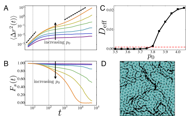
Figure 1: Analysis of glassy behavior. (A) The mean-squared displacement of cell centers for $D_{r}=1$ and $v_{0}=0.1$ and various values of $p_{0}$ (bottom to top: $p_{0}=3.5,3.65,3.7,3.75,3.8,3.85$) show the onset of dynamical arrest as $p_{0}$ is changed indicating a glass transition. The dashed lines indicate a slope of $2$(ballistic) and $1$(diffusive) on log-log plot. (B) The self-intermediate scattering function at the same values of $p_{0}$ shown in (A) shows the emergence of caging behavior at the glass transition. (C) The effective self-diffusivity as function of $p_{0}$ at $v_{0}=0.1$. At the glass transition $D_{eff}$ becomes nonzero. (D)The cell displacement map in SPV model for a fluid state very close to the glass transition ($p_{0}=3.8$, $v_{0}=0.1$ and $D_{r}=1$) over a time window $t=10^{4}$ corresponding to the structural relaxation at which $F_{s}(t)\approx 1/2$.

During many biological processes, however, a tissue remains at confluence (packing fraction equal to unity) while it changes from a liquid-like to a solid-like state or vice-versa. For example, in would healing, cells collectively organize to form a ‘moving sheet’ without any change in their packing density Kim_monoloayer_obstacle_2013 , and during vertebrate embryogenesis mesendoderm tissues are more fluid-like than ectoderm tissues, despite both having packing fraction equal to unity Schoetz2013 .

Recently, Bi and coworkers bi_manning_nphys have demonstrated that the well-studied vertex model for 2-D confluent tissues ngai_honda ; Farhadifar2007 ; Hufnagel2007 ; Staple2010 ; manning_2010 ; bi_softmatter exhibits a rigidity transition in the limit of zero cell motility. Specifically, the rigidity of the tissue vanishes at a critical balance between cortical tension and cell-cell adhesion. An important insight is that this transition depends sensitively on cell shapes, which are well-defined in the vertex model. While promising, vertex models are difficult to compare to some aspects of experiments because they do not incorporate cell motility.

In this work, we bridge the gap between the confluent tissue mechanics and cell motility by studying a hybrid between the vertex model and the SPP model, that we name Self-Propelled-Voronoi (SPV) model. A similar model was introduced by Li and Sun Li_Sun_Biophys , and cellular Potts models also bridge this gap Szabo_Potts_2010 ; Kabla_CPM , although glass transitions have not been carefully studied in any of these hybrid systems.

I The SPV model

While the vertex model describes a confluent tissue as a polygonal tiling of space where the degrees of freedom are the vertices of the polygons, the SPV model identifies each cell only using the center ($\bm{r}_{i}$) of Voronoi cells in a Voronoi tessellation of space (Dirichlet domains) Dirichlet_1850 . The observation that Voronoi tessellations can describe cellular patterns in epithelial tissues was first proposed by Honda honda_voronoi . For a tissue containing $N$-cells, the inter-cellular interactions are captured by a total energy which is the same as that in the vertex model. Since the tessellation is completely determined by the $\{\bm{r}_{i}\}$, the total tissue mechanical energy can be fully expressed as $E=E(\{\bm{r}_{i}\})$:

$$E=\sum_{i=1}^{N}\left[K_{A}(A(r_{i})-A_{0})^{2}+K_{P}(P(r_{i})-P_{0})^{2}\right].$$ (1)

The term quadratic in cell area $A(r_{i})$ results from a combination of cell volume incompressibility and the monolayer’s resistance to height fluctuations Hufnagel2007 . The term involving the cell perimeter $P(r_{i})$ originates from active contractility of the acto-myosin sub-cellular cortex (quadratic in perimeter) and effective cell membrane tension due to cell-cell adhesion and cortical tension (both linear in perimeter). This gives rise to an effective target shape index that is dimensionless: $p_{0}=P_{0}/\sqrt{A_{0}}$. $K_{A}$ and $K_{P}$ are the area and perimeter moduli, respectively. For the remainder of this manuscript we assume $p_{0}$ is homogenous across a tissue, although heterogeneous properties are also interesting to consider Wetzel_draft_2015 .

In the vertex model bi_manning_nphys , a rigidity transition takes place at a critical value of $p_{0}=p_{0}^{*}\approx 3.81$. When $p_{0}<p_{0}^{*}$, cortical tension dominates over cell-cell adhesion and the energy barriers for local cell rearrangement and motion are finite. The tissue then behaves as a elastic solid with finite shear modulus. When $p_{0}>p_{0}^{*}$, cell-cell adhesion dominates and the energy barriers for local rearrangements vanish, resulting in zero rigidity and fluid-like behavior. While the energy functional for cell-cell interactions is identical in the vertex and SPV models, the two are truly distinct: the local minimum energy states of the vertex model are not guaranteed to be similar to a Voronoi tessellation of cell centers, although we do find them to be very similar in practice. Therefore, we are also interested in whether a rigidity transition in the SPV model coincides with the rigidity transition of the vertex model.

We define the effective mechanical interaction force experienced by cell $i$ as $\bm{F}_{i}=-\bm{\nabla}_{i}E$ (see Appendix A for details). In contrast to particle-based models, $\bm{F}_{i}$ is non-local and non-additive: $\bm{F}_{i}$ cannot be expressed as a sum of pairwise force between cells $i$ and its neighboring cells. Nevertheless, one can show that momentum is still precisely conserved by this energy functional in the absence of the additional self-propulsion forces introduced below.

In addition to $\bm{F}_{i}$, cells can also move due to self-propelled motility. Just as in SPP models, we assign a polarity vector $\hat{\bm{n}}_{i}=(\cos\theta_{i},\sin\theta_{i})$ to each cell; along $\hat{\bm{n}}_{i}$ the cell exerts a self-propulsion force with constant magnitude $v_{0}/\mu$, where $\mu$ is the mobility (the inverse of a frictional drag). Together these forces control the over-damped equation of motion of the cell centers $\bm{r}_{i}$

$$\frac{d\bm{r}_{i}}{dt}=\mu\bm{F}_{i}+v_{0}\hat{\bm{n}}_{i}.$$ (2)

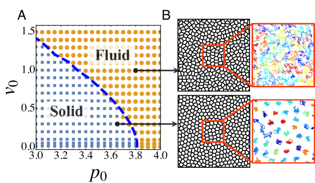
Figure 2: (A) Glassy phase diagram for confluent tissues as function of cell motility $v_{0}$ and target shape index $p_{0}$ at fixed $D_{r}=1$. Blue data points correspond to solid-like tissue with vanishing $D_{eff}$; orange points correspond to flowing tissues (finite $D_{eff}$). The dynamical glass transition boundary also coincides with the locations in phase space where the structural order parameter $q=\left\langle p/\sqrt{a}\right\rangle=3.81$ (dashed line). In the solid phase, $q\approx 3.81$ and $q>3.81$ in the fluid phase. (B) Instantaneous tissue snapshots show the difference in cell shape across the transition. Cell tracks also show dynamical arrest due to caging in the solid phase and diffusion in the fluid phase.

The polarity is a minimal representation of the front/rear characterization of a motile cell Szabo_Potts_2010 . While the precise mechanism for polarization in cell motility is an area of intense study, here we model its dynamics as a unit vector that undergoes random rotational diffusion

$$\begin{split}\partial_{t}\theta_{i}&=\eta_{i}(t)\\ \langle\eta_{i}(t)\eta_{j}(t^{\prime})\rangle&=2D_{r}\delta(t-t^{\prime})\delta_{ij}\end{split}$$ (3)

where $\theta_{i}$ is the polarity angle that defines $\hat{\bm{n}}_{i}$, and $\eta_{i}(t)$ is a white noise process with zero mean and variance $2D_{r}$. The value of angular noise $D_{r}$ determines the memory of stochastic noise in the system, giving rise to a persistence time scale $\tau=1/D_{r}$ for the polarization vector $\mathbf{\hat{n}}$. For small $D_{r}\ll 1$, the dynamics of $\mathbf{\hat{n}}$ is more persistent than the dynamics of the cell position. At large values of $D_{r}$, i.e. when $1/D_{r}$ becomes the shortest timescale in the model, Eq. (2) approaches simple Brownian motion.

The model can be non-dimensionalized by expressing all lengths in units of $\sqrt{A_{0}}$ and time in units of $1/(\mu K_{A}A_{0})$. There are three remaining independent model parameters: the self propulsion speed $v_{0}$, the cell shape index $p_{0}$, and the rotational noise strength $D_{r}$. We simulate a confluent tissue under periodic boundary conditions with constant number of $N=400$ cells (no cell divisions or apoptosis) and assume that the average cell area coincides with the preferred cell area, i.e. $\langle A_{i}\rangle=A_{0}$. This approximates a large confluent tissue in the absence of strong confinement. We numerically simulate the model using molecular dynamics by performing $10^{5}$ integration steps at step size $\Delta t=10^{-1}$ using Euler’s method. A detailed description of the SPV implementation can be found in the Appendix Sec. A.

II Characterizing glassy behavior

We first characterize the dynamics of cell motion within the tissue by analyzing the mean-squared displacement (MSD) of cell trajectories. In Fig. 1(a), we plot the MSD as function of time, for tissues at various values of $p_{0}$ and fixed $v_{0}=0.1$ and $D_{r}=1$. The MSD exhibits ballistic motion ( slope close to $2$ on a log-log plot) at short times, and plateaus at intermediate timescales. The plateau is an indication that cells are becoming caged by their neighbors. For large values of $p_{0}$, the MSD eventually becomes diffusive (slope =1), but as $p_{0}$ is decreased, the plateau persists for increasingly longer times. This indicates dynamical arrest due to caging effects and broken ergodicity, which is a characteristic signature of glassy dynamics.

Another standard method for quantifying glassy dynamics is the self-intermediate scattering function van_Hove_1954 : $F_{s}(k,t)=\left\langle e^{i\vec{k}\cdot\Delta\vec{r}(t)}\right\rangle.$ Glassy systems possess a broad range of relaxation timescales, which show up as a long plateau in $F_{s}(t)$ when it is analyzed at a lengthscale $q$ comparable to the nearest neighbor distance. Fig 1 (b) illustrates precisely this behavior in the SPV model, when $|\vec{k}|=\pi/r_{0}$, where $r_{0}$ is the position of the first peak in the pair correlation function. The average $\langle...\rangle$ is taken temporally as well as over angles of $\vec{k}$. $F_{s}(t)$ also clearly indicates that there is a glass transition as a function of $p_{0}$: at high $p_{0}$ values $F_{s}$ approaches zero at long times, indicating that the structure is changing and the tissue behaves as a viscoelastic liquid. At lower values of $p_{0}$, $F_{s}$ remains large at all timescales, indicating that the structure is arrested and the tissue is a glassy solid. Fig 1 (d) demonstrates that at the structural relaxation time, the cell displacements show collective behavior across large lengthscales suggesting strong dynamical heterogeneity. This is strongly reminiscent of the ‘swirl’ like collective motion seen in experiment in epithelial monolayers Angelini_PRL_2010 ; Angelini_PNAS_2011 ; Poujade_2007 ; Silberzan2010 ; Garcia_Gov_2015 .

II.1 A dynamical order parameter for the glass transition

Although the phase space for this model is three dimensional, we now study the model at a fixed value of $D_{r}=1$.

We then search for a dynamical order parameter that distinguishes between the glassy and fluid states as a function of the two remaining model parameters,$(v_{0},p_{0})$. A candidate order parameter is the self-diffusivity $D_{s}$: $D_{s}=\lim_{t\to\infty}\langle{\Delta r(t)}^{2}\rangle/(4t).$ For practicality, we calculate $D_{s}$ using simulation runs of $10^{5}$ time steps, chosen to be much longer than the typical caging timescale in the fluid regime. We present the self-diffusivity in units of $D_{0}=v_{0}^{2}/(2D_{r})$, which is the free diffusion constant of an isolated cell. $D_{eff}=D_{s}/D_{0}$ then serves as an accurate dynamical order parameter that distinguishes a fluid state from a solid (glassy) state in the space of $(v_{0},p_{0})$, matching the regimes identified using the MSD and $F_{q}$. In Fig. 2, the fluid region is characterized by a finite value of $D_{eff}$ and $D_{eff}$ drops below a noise floor of $\sim 10^{-3}$ as the glass transition is approached. In practice, we label materials with $D_{eff}>10^{-3}$ as fluids indicated by an orange dot, and those with $D_{eff}\leq 10^{-3}$ as solids indicated by blue squares. Importantly, we find that the SPV model in the limit of zero cell motility shares a rigidity transition with the vertex model bi_manning_nphys at $p_{0}\approx 3.81$, and that this rigidity transition controls a line of glass transitions at finite cell motilities. Typical cell tracks (Fig. 2) clearly show caging behavior in the glassy solid phase.

II.2 Cell shape is a structural order parameter for the glass transition

In glassy systems it can be difficult to experimentally distinguish between a truly dynamically arrested state and a state with relaxation times longer than the experimental time window. Similarly, in tissues it is experimentally challenging to quantify a glass transition through the measurement of a dynamical quantity such as the diffusivity $D_{s}$. Identifying a static quantity that directly probes the mechanical properties of a tissue would therefore be a powerful tool for experiments. Puliafito et al. have suggested that shape changes accompany dynamical arrest in proliferating tissues Puliafito_2012 . Similarly, a structural signature based on cell shapes – the shape index $q=\left\langle p/\sqrt{a}\right\rangle$ – was previously shown to be an excellent order parameter for the confluent tissue rigidity transition in the vertex model Park_2015 . In a model where cells were not motile ($v_{0}=0$) we found that when $p_{0}<3.813$, $q$ is constant $\sim 3.81$ and when $p_{0}>3.81$ $q$ grows linearly with $p_{0}$. Quite surprisingly, we found that the prediction of $q=3.813$ works perfectly in identifying a jamming transition in in-vitro experiments involving primary human tissues, where cells are clearly motile ($v_{0}\neq 0$) Park_2015 . At that time, we did not understand why the $v_{0}=0$ theory worked so well for these tissues.

The prediction of a solid-liquid transition in the SPV model presented here provides an explanation for this observation.We find that $q$ (which can be easily calculated in experiments or simulations from a snapshot) can be used as a structural order parameter for the glass transition for all values of $v_{0}$, not just at $v_{0}=0$. Specifically, the boundary defined by $q=3.813$, shown by the blue dashed line in Fig. 2(A) coincides extremely well with the glass transition line obtained using the dynamical order parameter, shown by the round and square data points. The insets to Fig. 2 also illustrate typical cell shapes: cells are isotropic on average in the solid phase and anisotropic in the fluid phase. This highlights the fact that $q$ can be used as a structural order parameter for the glass transition at all cell motilities, providing a powerful new tool for analyzing tissue mechanics.

III A three-dimensional jamming phase diagram for tissues

Having studied the glass transition as function of $v_{0}$ and $p_{0}$ at a large value of $D_{r}$, we next investigate the full three-dimensional phase diagram by characterizing the effect of $D_{r}$ on tissue mechanics and structure. $D_{r}$ controls the persistence time $\tau=1/D_{r}$ and persistence length or Péclet number $Pe\sim v_{0}/D_{r}$ of cell trajectories; smaller values of $D_{r}$ correspond to more persistent motion.

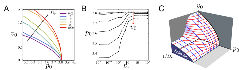
Figure 3: (A) The glass transition in $v_{0}-p_{0}$ phase space shifts as the persistence time changes. Lines represent the glass transition identified by the structural order parameter $q=3.81$. The phase boundary collapse to a single point at $p_{0}^{*}=3.81$, regardless of $D_{r}$, in the limit $v_{0}\rightarrow 0$. (B) The glass transition in $p_{0}-D_{r}$ phase space shifts as a function of $v_{0}$ (from top to bottom: $v_{0}=0.02,0.08,0.14,0.2,0.26$) For large $v_{0}$ there is a crossover in the behavior at $D_{r}\sim\mu K_{A}A_{0}=1$, as discussed in the main text. (C) The phase boundary between solid and fluid as function of motility $v_{0}$, persistence $1/D_{r}$ and $p_{0}$ which is tuned by cell-cell adhesion can be organized into a schematic 3D phase diagram. Red lines on the surface correspond to iso-$v_{0}$ contours and blue lines correspond to iso-$D_{r}$ contours.

In Fig. 3(A), we show several 2D slices of the three dimensional jamming boundary. Solid lines illustrate the phase transition line identified by the structural order parameter $q=3.813$ as function of $v_{0}$ and $p_{0}$ for a large range of $D_{r}$ values (from $10^{-2}$ to $10^{3}$). (In Appendix B.2 we demonstrate that the structural transition line $q=3.813$ matches the dynamical transition line for all studied values of $D_{r}$.) In contrast to results for particulate matter Berthier_PRL_2014 , this figure illustrates that the glass transition lines meet at a single point ($p_{0}=3.81$) in the limit of vanishing cell motility, regardless of persistence.

Fig. 3(B) shows an orthogonal set of slices of the jamming diagram, illustrating how the phase boundary shifts as function of $p_{0}$ and $D_{r}$ at various values of $v_{0}$. This highlights the interesting result that a solid-like material at high value of $D_{r}$ can be made to flow simply by lowering its value of $D_{r}$. The crossover in behavior at large $v_{0}$ occurs when the persistence time $1/D_{r}$ is approximately equal to the viscous relaxation time $1/(\mu K_{A}A_{0})=1$.

These slices can be combined to generate a three-dimensional jamming phase diagram for confluent biological tissues, shown in Fig. 3(C). This diagram provides a concrete, quantifiable prediction for how macroscopic tissue mechanics depends on single-cell properties such as motile force, persistence, and the interfacial tension generated by adhesion and cortical tension.

We note that Fig. 3(C) is significantly different from the jamming phase diagram conjectured by Sadati et al Sadati-Fredberg-review , which was informed by results from adhesive particulate matter Trappe_nature_2001 . For example, in particulate matter adhesion enhances solidification, while in confluent models adhesion increases cell perimeters/surface area and enhances fluidization. In addition, we identify “persistence” as a new axis with a potentially significant impact on cell migration rates in dense tissues.

Figure 4: (A-C) Instantaneous cell displacements at $p_{0}=3.65$ and $v_{0}=0.5$. They are different from the displacements shown in Fig. 1(D) which are averaged over the structural relaxation timescale. (A) At the lowest value of $D_{r}=0.01$, the cells are able to flow by collectively displacing along the ‘soft’ modes of the system (Appendix. B.1). (B) At $D_{r}=0.1$, collective displacements are less pronounced. (C) For $D_{r}=1$ and larger, the displacements appear disordered and uncorrelated.

To better understand why persistence is so important in dense tissues, we first have to characterize the transitions between different cellular structures. In the limit of zero cell motility, the system can be described by a potential energy landscape where each allowable arrangement of cell neighbors corresponds to a metastable minimum in the landscape. There are many possible pathways out of each metastable state: some of correspond to localized cell rearrangements, while others correspond to large-scale collective modes. The maximum energy required to transition out of a metastable state along each pathway is called an energy barrier bi_softmatter .

We observe that tissue fluidity can increase drastically with increasing $D_{r}$ at finite cell speeds. This suggests that different pathways (with lower energy barriers) must become dynamically accessible at higher values of $D_{r}$.

One hint about these pathways comes from the instantaneous cell displacements, shown for different values of $D_{r}$ in Fig. 4. At high values of $D_{r}$, ($p_{0}=3.78$, $v_{0}=0.1$) the instantaneous displacement field is essentially random and largely uncorrelated, as shown in Fig. 4, and the material is solid-like. There is no collective behavior among cells, and each cell ‘rattles’ independently near its equilibrium position.

However, as $D_{r}$ is lowered, the instantaneous displacement field becomes much more collective (Fig. 4) and the tissue begins to flow, presumably because these collective displacement fields correspond to pathways with lower transition energies.

Two obvious questions remain: How does a lower value of $D_{r}$ generate more collective instantaneous displacements? Why should collective instantaneous displacements generically have lower energy barriers? The first question can be answered by extending ideas first proposed by Henkes, Fily and Marchetti Henkes2011 to explain why motion in self-propelled particle models seems to follow the ‘soft modes’ of a solid. This argument is based on a simple, yet powerful observation: in the limit of zero motility ($v_{0}=0$), a solid-like state will have a well-defined set of normal modes of vibration (with frequencies $\{\omega_{\nu}\}$), and a corresponding set of eigenvectors ($\{\hat{e}_{\nu}\}$) that forms a complete basis. At higher motilities ($v_{0}>0$) near the glass transition, the motion of particles in the system can be expanded in terms of the eigenvectors. As discussed in Appendix B.1, one can use this observation to show that in the limit of $D_{r}\to 0$, motion along the lowest frequency eigenmodes is amplified – the amplitude along each mode is proportional to $1/\omega_{\nu}^{2}$. These low-frequency normal modes are precisely the collective displacements observed for low $D_{r}$.

The second question is more difficult to answer because it is impossible to enumerate all of the possible transition pathways and energy barriers in a disordered material. However, a partial answer comes from recent work in disordered particulate matter showing that low-frequency normal modes do have significantly lower energy barriers Xu_EPL_2010 ; Manning_Liu_PRL_2011 than higher frequency normal modes. A similar analysis could potentially be performed in vertex or SPV models.

IV A continuum model for glass transitions in tissues

Although continuum hydrodynamic equations of motion have been developed by coarse graining SPP models in the dilute limit, there is no existing continuum model for a dense active matter system near a glass transition. Here we propose that a simple trap bouchaud_trap or Soft Glassy Rheology (SGR) Sollich_SGR_1998 model provides an excellent continuum approximation for the phase behavior in the large $D_{r}$ Brownian regime, but fails in the small $D_{r}$ limit.

For large $D_{r}$ it is known that particle behave like Brownian particles with an effective temperature $T_{eff}=v_{0}^{2}/2\mu D_{r}$ Fily_2012 . This mapping becomes exact when $D_{r}\rightarrow\infty$ at fixed “effective inertia” $(\mu D_{r})^{-1}$ Fily_SM_2014 . In other words, like in granular systems Abate_Durian_effective_temp ; Cecconi_PRL_2003 , the effective temperature in SPP is dominated by kinetic effects. Guided by this result we conjecture that in our model the temperature also scale quadratically with the velocity,

$$T_{eff}\propto cv_{0}^{2}.$$ (4)

Physically, this effective temperature gives the amount of energy available for individual cells to vibrate within their cage or ‘trap’.

The next important question is how to characterize the ‘trap depths’, or energy barriers between metastable states. In the Brownian regime (large $D_{r}$) there is no dynamical mechanism for the cells to organize collectively, and therefore a reasonable assumption is that the rearrangements are small and localized.

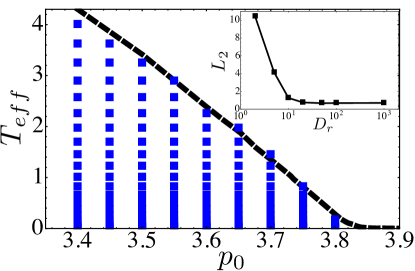
Figure 5: Comparison between SPV glass transition and an analytic prediction based on a Soft Glass Rheology (SGR) continuum model. The dashed line corresponds to an SGR prediction with no fit parameter based on previously measured vertex model trap depths bi_softmatter . Data points correspond to SPV simulations with $D_{r}=10^{-3}$ and where we have defined $T_{eff}=cv_{0}^{2}$ with $c=0.1$ as the best-fit normalization parameter. Blue points correspond to simulations which are solid-like, with $D_{eff}<10^{-3}$, and the boundary of these points define the observed SPV glass transition line. (Inset) $L_{2}$ difference between SPV glass transition line (at best-fit value of $c$) and the predicted SGR transition line at various values of $D_{r}$. The SGR prediction based on localized T1 trap depths works well in the high $D_{r}$ limit, but not in the low $D_{r}$ limit.

In bi_softmatter , some of us explicitly calculated the statistics of energy barriers for localized rearrangements in the equilibrium vertex model. In the 2D vertex model, one can show that localized rearrangements must occur via so-called T1 transitions Weaire_book . Using a trap model bouchaud_trap or Soft Glassy Rheology(SGR) Sollich_SGR_1998 framework, we were able to use these statistics to generate an analytic prediction, with no fit parameters, for the glass transition temperature $T_{g}$ as function of $p_{0}$.

To see if the SGR prediction for the glass transition holds for the SPV model in the large $D_{r}$ limit, we simply overlay the data points corresponding to glassy states from the SPV model with the glass transition $T_{g}$ line predicted in bi_softmatter . There is one fitting parameter $c$ that characterizes the proportionality constant in Eq. 4. Fig 5, shows that the SPV data for $D_{r}=10^{3}$ is in excellent agreement with our previous SGR prediction. Because $T_{eff}\sim v_{0}^{2}$, and the glass transition line scales as $T_{g}\sim p_{0}^{*}-p_{0}$ for $p_{0}\ll p_{0}^{*}$ and $D_{r}\to 0$, the glass transition line scales as $v_{0}\sim{(p_{0}^{*}-p_{0})}^{0.5}$ in those limits.

The reason the effective temperature SGR model works here is that, like in SPP models of spherical active Brownian colloids, the angular dynamics of each cell evolves independently of cell-cell interactions and of the angular dynamics of other cells. An additional alignment interaction that couples the angular and translational dynamics may therefore modify this behavior.

To our knowledge, this is the first time that a SGR / trap model prediction has been precisely tested in any glassy system. This is because, unlike most glass models, we can enumerate all of the trap depths for localized transition paths in the vertex model.

However, for small values of $D_{r}$, we have shown that cell displacements are dominated by collective normal modes, and therefore the energy barriers for localized T1 transitions are probably irrelevant in this regime. The inset to Fig 5 shows the deviation ($L^{2}$-norm) between glass transition lines in the SPV model and T1-based SGR prediction as a function of $D_{r}$. We see that the SGR prediction fails in the small $D_{r}$ limit, as expected. A better understanding of the energy barriers associated with collective modes will be required to modify the theory at small $D_{r}$.

V Discussion and Conclusions

We have shown that a minimal model for confluent tissues with cell motility exhibits glassy dynamics at constant density. This model allows us to make a quantitative prediction for how the fluid-to-solid/jamming transition in biological tissues depends on parameters such as the cell motile speed, the persistence time associated with directed cell motion, and the mechanical properties of the cell (governed by adhesion and cortical tension). We define a simple, experimentally accessible structural order parameter – the cell shape index – that robustly identifies the jamming transition, and we show that a simple analytic model based on localized T1 rearrangements precisely predicts the jamming transition in the large $D_{r}$ limit. We also show that this prediction fails in the small $D_{r}$ limit, because the instantaneous particle displacements are dominated by collective normal modes.

This model makes several experimentally-verifiable predictions for cell shape and tissue mechanics:

• The order parameter $q=3.81$ is a structural signature for the glass transition, even in tissues with significant cell motility or dynamics. This prediction has already been tested in epithelial lung tissue Park_2015 , but it should be much more broadly applicable. We have performed a rudimentary shape analysis of a small number of images from other systems that have been previously published, including proliferating MCDK monolayers Deforet_ncomm_2014 and convergent extension in fruit fly development matthias_elife and found that the shapes are consistent with this prediction. A much more careful analysis with full data sets should be performed to further validate this prediction or understand where it breaks down.

• In the limit of vanishing cell motility, shape and pressure fluctuations should vanish when the jamming transition is approached from the solid side, and remain zero in the fluid. A finite motility $v_{0}$ will induce such fluctuations in the fluid phase, as confirmed by preliminary calculation of cellular stresses and pressure in the SPV model SPV_stress_paper . This could be studied by combining measurement of cell shape fluctuations with traction force microscopy (TFM) in wound healing assays. After locating the glass transition by imaging cell shape changes, it may be possible to extract information on cell motility $v_{0}$ from cellular stresses and pressure inferred from TFM in the fluid phase near the glass transition. This suggests that one may estimate cell motility by examining the changes in cellular stresses and pressure in the cell monolayer near the unjamming transition and assuming that the local velocity of the monolayer is very small just above the transition. The latter assumption can also be verified independently via particle image velocimetry (PIV).

• Cell proliferation, so far neglected in our model, causes an increase in cell number density in confluent tissues. Often this is accompanied by a reduction in individual cell motility $v_{0}$, via contact inhibition of locomotion. In cases where this is the dominant effect and changes to the ratio between $A_{0}$ and $P_{0}$ are negligible, our work predicts that proliferation would drive the system towards jamming. This is consistent with existing reports in the literature Deforet_ncomm_2014 , although more work is required to test the prediction carefully. In tissues where $v_{0}$ remains low at all times Puliafito_2012 , our model predicts that proliferation can either cause jamming or unjamming, depending on whether cell divisions are oriented in such a way to decrease or increase cell shape anisotropy.

• Spatial correlations and fluctuations of the cell displacement field, such as swirl sizes  Poujade_2007 ; Silberzan2010 ; Angelini_PRL_2010 ; Angelini_PNAS_2011 ; Garcia_Gov_2015 , should grow as a tissue approaches the glass transition from the fluid side. Very recently, a similar prediction for displacements and correlation lengths based on a particle-based model has been verified in one cell type Garcia_Gov_2015 . The SPV model, which makes predictions for cell shapes in addition to displacements and correlation lengths, could be tested simply by compiling detailed statistics about cell shapes and cell motion in epithelial monolayers.

Although all of the work presented here focuses on the SPV model, which tracks cell centers and therefore has only two degrees of freedom per cell, we found that in the limit of zero cell motility it exhibits the same rigidity transition as the vertex model which has two degrees of freedom per vertex. We have also checked that an ”active vertex model”, where active motile forces are added to the vertex model vertices, also exhibits a robust glass transition characterized by the shape order parameter $q$. The fact that two models with ostensibly different degrees of freedom share the same transition suggests that there is a deeper universality, perhaps generated by isostaticity, that remains to be understood.

Another result of this work is the surprising and unexpected differences between confluent models (such as the vertex and SPV models) and particle-based models (such as Lennard-Jones glasses and SPP models). For example, works by Berthier Berthier_PRL_2014 , Fily and Marchetti Fily_2012 in SPP models suggest that the location of the zero motility glass transition packing density $\phi_{G}$ (defined as the density at which dynamics cease in the limit of $v_{0}\to 0$) depends the value of noise, $D_{r}$. This is also related to the observation that the jamming and glass transition are not controlled by the same critical point in non-active systems Ikeda_PRL_2012 ; Teitel_athermal_vs_glass . We find this is not the case in the SPV model. Fig. 3(a & b) show that while the glass transition point $p_{0}^{*}$ shifts with $D_{r}$ at finite values of $v_{0}$, in the limit of vanishing motility, all glass transition lines merge on to a single point in the limit $v_{0}\to 0$, namely $p_{0}^{*}=3.81$.

Given these differences, it is important to ask which type of model is appropriate for a given system. We argue that SPV models are maybe more appropriate for many biological tissues. Whereas SPP models interact with two-body interactions that only depend on particle center positions, both SPV and vertex models naturally incorporate contractility as a key property of living cells and capture the inherently multi-body nature of intercellular forces due to shape deformations. Unlike equilibrium vertex models, SPV models account for cell motility, and they are also much easier to simulate in 3D (which is nearly impossible in practice for the vertex model.)

Recent work by Li and Sun Li_Sun_Biophys also models a confluent cell as a Voronoi tessellation of the plane. An important difference between this work and ours is that in Ref.  Li_Sun_Biophys cell-cell adhesion is captured via a potential that is quadratic in the distance between cell centers, just as in particle models. We might guess that stronger cell-cell adhesion in their model will result in stiffening of the tissue, which is common for particle based models, although that remains to be tested in active systems. In contrast, adhesion enters our model through the coupling of the shape energy to the cell perimeter. Increasing cell-cell adhesion (or decreasing cortical tension) yields a larger value of $p_{0}$, which leads to the tissue becoming softer.

We expect that other shape-based models of confluent tissue dynamics will also yield the glass transition described here. For example, it has been reported in recent works based on the Cellular Potts model Szabo_Potts_2010 ; Kabla_CPM and in a modified SPP model Garcia_Gov_2015 when the cell motile force is decreased beyond a certain threshold, the motion of cells transitions from diffusive to sub-diffusive. This is similar to crossing the glass transition line in the SPV model by decreasing the value of $v_{0}$.

In this work and in previous work based on the vertex model, the cell volume is generally assumed to be fixed. While this is a good assumption in developmental systems such as drosopholia Zallen_Karen ; Gelbart_PNAS_2012 and zebrafish manning_2010 , epithelial tissues cells can show significant volume fluctuations, as reported recently  Zehnder_Angelini_Biophys_2015 ; Zehnder_Angelini_PRE_2015 . Therefore, it will be important to incorporate volume fluctuations in future iterations of the vertex model or the SPV model, as they introduce another source of active shape fluctuation and could therefore lead to jamming or unjamming of the tissue locally and potentially shift the location of the rigidity and glass transitions.

In our version of the SPV model, we have assumed that cell polarity is controlled by simple rotational white noise. It is also possible to include more complex mechanisms. For example, external chemical or mechanical cues could be modeled by coupling $v_{0}$ and $\hat{\bm{n}}_{i}$ to chemoattractant or mechanical gradients, allowing waves or other pattern formation mechanisms to interact with the jamming transition. Similarly, simple alignment rules (such as those in the Viscek model Vicsek_1995 ) could lead to collective flocking modes that also affect glassy dynamics.

Another interesting extension of the SPV model would be to study the role of cell-cell friction, which has already been shown to be important in controlling collective dynamics in particle-based tissue models Garcia_Gov_2015 . Our current model includes viscous frictional coupling of cell to the 2D substrate and cell-cell adhesion enters as a negative line tension on interfaces. However, it would be possible to add a frictional force between cells proportional to the length of the edge shared between two cells, and we know from previous work on particulate glasses that these localized frictions can change the location of jamming/glass transition and the nature of spatial correlations in a glass Silbert_frictional_jamming ; Henkes_frictional_jamming .

It is also tempting to speculate about the relationship between the unjamming transition captured by our model and the epithelial-mesenchimal transition (EMT) that precedes cell escape from a solid tumor mass. The EMT involves significant changes in cell-cell adhesion and cytoskeletal composition, with associated changes in cell shape and motility. This suggests that escape from the tumor mass is controlled not just by the chemical breakdown of the basement membrane, but also by specific changes in mechanical properties of both individual cells and the surrounding tissue Wong_Nat_Mat_2014 . One could then hypothesize that the collective unjamming described here may provide the first necessary step towards the mechanical changes needed for cell escape from primary tumors.

In particular, recent work suggests that cancer tumors are mechanically heterogeneous, with mixtures of stiff and soft cells that have varying degrees of active contractility Wetzel_draft_2015 . Our jamming phase diagram suggests that the soft cells, which often exhibit mesenchymal markers and presumably correspond to higher values of $p_{0}$, might unjam and move towards the boundary of a primary tumor more easily than their stiff counterparts. Examining the effects of tissue heterogeneity on tissue rigidity and patterns of cell motility is therefore a very promising avenue for developing predictive theories for tumor invasiveness and metastasis.

Appendix A Simulation algorithm for the SPV model

To create an initial configuration for the simulation, we first generate a seed point pattern using random sequential addition (RSA) RSA_Torquato and anneal it by integrating Eq. 2 with $v_{0}=0$ for $100$ MD steps. The resulting structure then serves as an initially state for all simulations runs. The use of (RSA) only serves to speed up the initial seed generation as using a Poisson random point pattern does not change the results presented in this paper.

At each time step of the simulation, a Voronoi tesselation is created based on the cell centers. The intercellular forces are then calculated based on shapes and topologies of the Voronoi cells (see discussion below). We employ Euler’s method to carry out the numerical integration of Eq. 2, i.e., at each time step of the simulation the intercellular forces is calculated based on the cell center positions in the previous time step.

In a Delaunay triangulation, a trio of neighboring Voronoi centers define a vertex of a Voronoi polygon. For example in Fig. 6, ($\vec{r}_{i},\vec{r}_{j},\vec{r}_{k}$) define the vertex $\vec{h}_{3}$, which is given by

$$\vec{h}_{3}=\alpha\vec{r}_{i}+\beta\vec{r}_{j}+\gamma\vec{r}_{k},$$ (5)

where the coefficients are given by

$$\begin{split}\alpha&={\|\vec{r}_{j}-\vec{r}_{k}\|}^{2}(\vec{r}_{i}-\vec{r}_{j})\cdot(\vec{r}_{i}-\vec{r}_{k})/D\\ \beta&={\|\vec{r}_{i}-\vec{r}_{k}\|}^{2}(\vec{r}_{j}-\vec{r}_{i})\cdot(\vec{r}_{j}-\vec{r}_{k})/D\\ \gamma&={\|\vec{r}_{i}-\vec{r}_{j}\|}^{2}(\vec{r}_{k}-\vec{r}_{i})\cdot(\vec{r}_{k}-\vec{r}_{j})/D\\ D&=2{\|(\vec{r}_{i}-\vec{r}_{j})\times(\vec{r}_{j}-\vec{r}_{k})\|}^{2}.\end{split}$$ (6)

Figure 6: Cell centers positions are specified by vectors $\{\vec{r}\}$. They form a Delaunay triangulation (black lines). Its dual is the Voronoi tessellation (red lines), with vertices given by $\{\vec{h}\}$.

In the vertex model, the total mechanical energy of a tissue depends only on the areas and perimeters of cells:

$$E=\sum_{i=1}^{N}\left[K_{P}(A_{i}-A_{0})^{2}+K_{P}(P_{i}-P_{0})^{2}\right].$$ (7)

In a Voronoi tessellation, the area and perimeter of a cell $i$ can be calculated in terms of the vertex positions

$$\begin{split}P_{i}&=\sum_{m=0}^{z_{i}-1}\|\vec{h}_{m}-\vec{h}_{m+1}\|;\\ A_{i}&=\frac{1}{2}\sum_{m=0}^{z_{i}-1}\|\vec{h}_{m}\times\vec{h}_{m+1}\|,\end{split}$$ (8)

where $z_{i}$ is the number of vertices for cell $i$ (also number of neighboring cells) and $m$ indexes the vertices. We use the convention $\vec{h}_{z_{i}}=\vec{h}_{0}$.

With these definitions, the total force on cell-$i$ can be calculated using Eq. 7

$$F_{i\mu}\equiv-\frac{\partial{E}}{\partial r_{i\mu}}=-\sum_{j\in n.n.(i)}\frac{\partial{E_{j}}}{\partial r_{i\mu}}-\frac{\partial{E_{i}}}{\partial r_{i\mu}},$$ (9)

here $\mu$ denotes the cartesian coordinates ($x,y$). The first term on the r.h.s. of Eq. 9 sums over all nearest neighbors of cell $i$. It is the force on cell $i$ due to changes in neighboring cell shapes. The second term is the force on cell $i$ due to shape changes brought on by its own motion.

It maybe tempting to treat $\frac{\partial{E_{j}}}{\partial r_{i\mu}}$ as the force between cells-$i$ and $j$, but

$$\frac{\partial{E_{j}}}{\partial r_{i\mu}}\neq\frac{\partial{E_{i}}}{\partial r_{j\mu}}$$ (10)

since the interaction is inherently multi-cellular in nature and interactions between $i$ and $j$ also depend on $k$ and $l$ (see Fig. 6).

For the typical configuration shown in Fig. 6, the first term in Eq. 9 can be expanded using the chain rule and calculated using Eq. 5

$$\begin{split}\frac{\partial{E_{j}}}{\partial r_{i\mu}}&=\sum_{\nu}\left(\frac{\partial{E_{j}}}{\partial h_{2\nu}}\frac{\partial h_{2\nu}}{\partial r_{i\mu}}+\frac{\partial{E_{j}}}{\partial h_{3\nu}}\frac{\partial h_{3\nu}}{\partial r_{i\mu}}\right).\end{split}$$ (11)

In Eq. 11, only terms involving $\vec{h}_{2}$ and $\vec{h}_{3}$ are kept since $E_{j}$ does not depend on other vertices of cell $i$. $\nu$ is a cartesian coordinate index. The energy derivative in Eq. 11 can be calculated in a straightforward way, by using Eqs. 7 and 8

$$\begin{split}\frac{\partial{E_{j}}}{\partial h_{2x}}=&2K_{A}(A_{j}-A_{0})\frac{\partial{A_{j}}}{\partial h_{2x}}+2K_{P}(P_{j}-P_{0})\frac{\partial{P_{j}}}{\partial h_{2x}}\\ =&K_{A}(A_{j}-A_{0})(h_{3y}-h_{7y})\\ &+2K_{P}(P_{j}-P_{0})\left(\frac{h_{2x}-h_{7x}}{\|\vec{h}_{7}-\vec{h}_{2}\|}+\frac{h_{2x}-h_{3x}}{\|\vec{h}_{2}-\vec{h}_{3}\|}\right)\\ \end{split}$$ (12)

and

$$\begin{split}\frac{\partial{E_{j}}}{\partial h_{2y}}=&2K_{A}(A_{j}-A_{0})\frac{\partial{A_{j}}}{\partial h_{2y}}+2K_{P}(P_{j}-P_{0})\frac{\partial{P_{j}}}{\partial h_{2y}}\\ =&K_{A}(A_{j}-A_{0})(h_{3x}-h_{7x})\\ &+2K_{P}(P_{j}-P_{0})\left(\frac{h_{2y}-h_{7y}}{\|\vec{h}_{7}-\vec{h}_{2}\|}+\frac{h_{2y}-h_{3y}}{\|\vec{h}_{2}-\vec{h}_{3}\|}\right).\\ \end{split}$$ (13)

Similarly, the second term on the r.h.s. of Eq. 9 can be calculated in a similar way.

Appendix B Cell displacements and structural order parameter as a function of $D_{r}$

B.1 Expanding cell displacements in an eigenbasis associated with the underlying dynamical matrix

In the absence of activity ($v_{0}=0$), the tissue is a solid for $p_{0}<p_{0}^{*}=3.81$. As $v_{0}$ is increased, the solid behavior persists up to $v_{0}=v_{0}^{*}(p_{0})$, which is given by the glass transition line in Fig. 2. In order for the tissue to flow, sufficient energy input is needed to overcome energy barriers in the potential energy landscape, which are a property of the underlaying solid state at $v_{0}=0$. In this limit, the instantaneous cell center positions $\{\vec{r}_{i}(t)\}$ can be thought of as a small displacement $\{\vec{d}_{i}(t)\}$ from the nearest solid reference state $\{\vec{r}_{0i}\}$ Henkes2011 where $\vec{d}_{i}(t)=\vec{r}_{i}-\vec{r}_{0i}$. The $\vec{r}_{0i}$ correspond to positions of cell in a solid, which has a well-defined linear response regime bi_manning_nphys . The linear response is most conveniently expressed as the eigen-spectrum of the dynamical matrix $D_{ij\alpha\beta}$. Since the eigenvectors $\{\hat{e}_{i,\nu}\}$ of $D_{ij\alpha\beta}$ form a complete orthonormal basis, the cell center displacement can then be expressed as a linear combination of $\{\hat{e}_{i,\nu}\}$

$$\vec{d}_{i}(t)=\sum_{\nu}a_{\nu}(t)\hat{e}_{i,\nu}$$ (14)

For simplicity, we will adopt the Bra-ket notation and express the eigenbasis simply as $|\nu\rangle$ and Eq. 14 becomes

$$|d\rangle=\sum_{\nu}a_{\nu}(t)|\nu\rangle,$$ (15)

where

$$\hat{D}|\nu\rangle=\omega_{\nu}^{2}|\nu\rangle$$ (16)

and $\omega_{\nu}^{2}$ are the eigenvalues of the dynamical matrix.

The polarization vector $\hat{n}_{i}$ can also be expressed as a linear combination of eigenvectors

$$|n\rangle=\sum_{\nu}b_{\nu}(t)|\nu\rangle.$$ (17)

Since the polarization vector and eigenvector are both unit vectors, it follows that $b_{\nu}(t)=\langle n|\nu\rangle=cos(\theta_{\nu}-\psi)$. Where $\psi$ is the angle of the polarization and $\theta_{\nu}$ the angle of the eigenvector.

Then the equation of motion for $\vec{d}_{i}$ (Eq. 2), can be rewritten as

$$\dot{\vec{d}}=-\mu\frac{\partial E}{\partial\vec{r}_{i}}\bigg{|}_{\vec{r}_{0,i}}+v_{0}\hat{n}_{i}$$ (18)

Using Eqs. 15–18, we find

$$\begin{split}\frac{d}{dt}\langle\nu|d\rangle&=-\mu\langle\nu|\hat{D}\ d\rangle+v_{0}\langle\nu|n\rangle\ \ ,\text{or}\\ \frac{d}{dt}a_{\nu}(t)&=-\mu\omega_{\nu}^{2}a_{\nu}(t)+v_{0}b_{\nu}(t).\end{split}$$ (19)

Then the equation of motion for each amplitude is

$$\begin{split}\frac{d}{dt}a_{\nu}(t)&=-\mu\omega_{\nu}^{2}a_{\nu}(t)+v_{0}cos(\theta_{\nu}-\psi)\\ \dot{\psi}&=\eta.\end{split}$$ (20)

This is just the equation of motion for a self-propelled particle tethered to a spring with active forcing that is strongest along the direction of the eigenvector Gov_elastic_gel_PRE_2015 . The solution is then:

$$a_{\nu}(t)=a_{\nu}(t=0)e^{-kt}+v_{0}\int_{0}^{t}dt^{\prime}e^{-k(t-t^{\prime})}cos(\theta_{\nu}-\psi),$$ (21)

where $k=\mu\omega_{\nu}^{2}$.

Solving for the ensemble averaged quantity:

$$\langle a_{\nu}(t)\rangle=a_{\nu}(t=0)e^{-kt}+v_{0}\int_{0}^{t}dt^{\prime}e^{-k(t-t^{\prime})}\langle cos(\theta_{\nu}-\psi)\rangle,$$ (22)

and using the relations

$$\begin{split}\langle\cos\psi(t)\rangle&=\cos\psi(0)e^{-D_{r}t};\\ \langle\sin\psi(t)\rangle&=\sin\psi(0)e^{-D_{r}t}\\ \cos(\theta_{\nu}-\psi)&=\sin(\theta_{\nu})\sin(\psi)+\cos(\theta_{\nu})\cos(\psi),\end{split}$$ (23)

to get the ensemble averaged solution for the amplitude becomes

$$\langle a_{\nu}(t)\rangle=a_{\nu}(0)e^{-kt}+v_{0}\cos\left(\theta_{\nu}-\psi(0)\right)\frac{e^{-kt}-e^{-D_{r}t}}{D_{r}-k}.$$ (24)

In the limit of $D_{r}\to\infty$ and Eq. 24 becomes

$$\langle a_{\nu}(t)\rangle=a_{\nu}(0)e^{-kt}.$$ (25)

This suggests that while normal modes control the rate of decay, they do no affect the long-time behavior.

However as $D_{r}\to 0$, Eq. 24 becomes

$$a_{\nu}(t)=a_{\nu}(0)e^{-\mu\omega_{\nu}^{2}t}+\frac{v_{0}}{\mu\omega_{\nu}^{2}}\cos\left(\theta_{\nu}-\psi(0)\right)\left(1-e^{-\mu\omega_{\nu}^{2}t}\right)$$ (26)

The second term in this equation scales as $\sim 1/\omega_{\nu}^{2}$. Therefore, at short times (corresponding to instantaneous response), the mode amplitude $a_{\nu}$ is much larger for modes at lower frequencies. Since the reference state is an elastic solid with Debye scaling $D(\omega)\sim\omega$ as $\omega\to 0$ bi_manning_nphys , this suggests that the displacement will be heavily dominated by the lowest frequency modes that are spatially more collective in nature.

B.2 Effect of $D_{r}$ on glass transition boundary

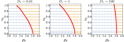
Figure 7: Comparison between glass transition boundaries obtained using shape order parameter (red line) and $D_{eff}$ (blue squares and orange circles).

Figure. 7 shows that the location in phase space where the shape index $q=3.81$ is in excellent agreement with the dynamical solid-fluid phase boundary determined by $D_{eff}$, at all values of $D_{r}$.

- [1] A. R. Abate and D. J. Durian. Effective temperatures and activated dynamics for a two-dimensional air-driven granular system on two approaches to jamming. Phys. Rev. Lett., 101:245701, Dec 2008.
- [2] Thomas E. Angelini, Edouard Hannezo, Xavier Trepat, Jeffrey J. Fredberg, and David A. Weitz. Cell migration driven by cooperative substrate deformation patterns. Phys. Rev. Lett., 104:168104, Apr 2010.
- [3] Thomas E. Angelini, Edouard Hannezo, Xavier Trepat, Manuel Marquez, Jeffrey J. Fredberg, and David A. Weitz. Glass-like dynamics of collective cell migration. Proceedings of the National Academy of Sciences, 108(12):4714–4719, 2011.
- [4] Julio M. Belmonte, Gilberto L. Thomas, Leonardo G. Brunnet, Rita M. C. de Almeida, and Hugues Chaté. Self-propelled particle model for cell-sorting phenomena. Phys. Rev. Lett., 100:248702, Jun 2008.
- [5] E. Ben-Isaac, É. Fodor, P. Visco, F. van Wijland, and Nir S. Gov. Modeling the dynamics of a tracer particle in an elastic active gel. Phys. Rev. E, 92:012716, Jul 2015.
- [6] Ludovic Berthier. Nonequilibrium glassy dynamics of self-propelled hard disks. Physical Review Letters, 112(22):220602, 2014.
- [7] Dapeng Bi, J. H. Lopez, J. M. Schwarz, and M. Lisa Manning. A density-independent rigidity transition in biological tissues. Nat Phys, advance online publication:–, 09 2015.
- [8] Dapeng Bi, Jorge H. Lopez, J. M. Schwarz, and M. Lisa Manning. Energy barriers and cell migration in densely packed tissues. Soft Matter, 10:1885–1890, 2014.
- [9] Fabio Cecconi, Andrea Puglisi, Umberto Marini Bettolo Marconi, and Angelo Vulpiani. Noise activated granular dynamics. Phys. Rev. Lett., 90:064301, Feb 2003.
- [10] M. Deforet, V. Hakim, H. G. Yevick, G. Duclos, and P. Silberzan. Emergence of collective modes and tri-dimensional structures from epithelial confinement. Nat Commun, 5, 05 2014.
- [11] Raphaël Etournay, Marko Popović, Matthias Merkel, Amitabha Nandi, Corinna Blasse, Benoît Aigouy, Holger Brandl, Gene Myers, Guillaume Salbreux, Frank Jülicher, and Suzanne Eaton. Interplay of cell dynamics and epithelial tension during morphogenesis of the Drosophila pupal wing. eLife, 4:e07090, jun 2015.
- [12] Reza Farhadifar, Jens-Christian Roeper, Benoit Aigouy, Suzanne Eaton, and Frank Julicher. The influence of cell mechanics, cell-cell interactions, and proliferation on epithelial packing. Current Biology, 17(24):2095 – 2104, 2007.
- [13] Yaouen Fily, Silke Henkes, and M. Cristina Marchetti. Freezing and phase separation of self-propelled disks. Soft Matter, 10:2132–2140, 2014.
- [14] Yaouen Fily and M. Cristina Marchetti. Athermal phase separation of self-propelled particles with no alignment. Phys. Rev. Lett., 108:235702, Jun 2012.
- [15] Simon Garcia, Edouard Hannezo, Jens Elgeti, Jean-François Joanny, Pascal Silberzan, and Nir S. Gov. Physics of active jamming during collective cellular motion in a monolayer. Proceedings of the National Academy of Sciences, 112(50):15314–15319, 2015.
- [16] Michael A. Gelbart, Bing He, Adam C. Martin, Stephan Y. Thiberge, Eric F. Wieschaus, and Matthias Kaschube. Volume conservation principle involved in cell lengthening and nucleus movement during tissue morphogenesis. Proceedings of the National Academy of Sciences, 109(47):19298–19303, 2012.
- [17] N.P.A.Devika Gunasinghe, Alan Wells, ErikW. Thompson, and HonorJ. Hugo. Mesenchymal–epithelial transition (met) as a mechanism for metastatic colonisation in breast cancer. Cancer and Metastasis Reviews, 31(3-4):469–478, 2012.
- [18] Anna Haeger, Marina Krause, Katarina Wolf, and Peter Friedl. Cell jamming: Collective invasion of mesenchymal tumor cells imposed by tissue confinement. Biochimica et Biophysica Acta (BBA) - General Subjects, 1840(8):2386 – 2395, 2014. Matrix-mediated cell behaviour and properties.
- [19] S. Henkes, M. van Hecke, and W. van Saarloos. Critical jamming of frictional grains in the generalized isostaticity picture. EPL (Europhysics Letters), 90(1):14003, 2010.
- [20] Silke Henkes, Yaouen Fily, and M. Cristina Marchetti. Active jamming: Self-propelled soft particles at high density. Phys. Rev. E, 84:040301, Oct 2011.
- [21] Hisao Honda. Description of cellular patterns by dirichlet domains: The two-dimensional case. Journal of Theoretical Biology, 72(3):523 – 543, 1978.
- [22] Lars Hufnagel, Aurelio A. Teleman, H. Rouault, Stephen M. Cohen, and Boris I. Shraiman. On the mechanism of wing size determination in fly development. Proceedings of the National Academy of Sciences, 104(10):3835–3840, March 2007.
- [23] Atsushi Ikeda, Ludovic Berthier, and Peter Sollich. Unified study of glass and jamming rheology in soft particle systems. Phys. Rev. Lett., 109:018301, Jul 2012.
- [24] Alexandre J. Kabla. Collective cell migration: leadership, invasion and segregation. Journal of The Royal Society Interface, 9(77):3268–3278, 2012.
- [25] Karen E Kasza, Dene L Farrell, and Jennifer A Zallen. Spatiotemporal control of epithelial remodeling by regulated myosin phosphorylation. Proc Natl Acad Sci U S A, 111(32):11732–11737, Aug 2014.
- [26] Jae Hun Kim, Xavier Serra-Picamal, Dhananjay T. Tambe, Enhua H. Zhou, Chan Young Park, Monirosadat Sadati, Jin-Ah Park, Ramaswamy Krishnan, Bomi Gweon, Emil Millet, James P. Butler, Xavier Trepat, and Jeffrey J. Fredberg. Propulsion and navigation within the advancing monolayer sheet. Nat Mater, 12(9):856–863, 09 2013.
- [27] G. Lejeune Dirichlet. Über die reduction der positiven quadratischen formen mit drei unbestimmten ganzen zahlen. Journal fur die reine und angewandte Mathematik, 40:209–227, 1850.
- [28] Bo Li and Sean X. Sun. Coherent motions in confluent cell monolayer sheets. Biophysical Journal, 107(7):1532–1541, 2015/08/23 2015.
- [29] Andrea J. Liu and Sidney R. Nagel. The jamming transition and the marginally jammed solid. Annual Review of Condensed Matter Physics, 1(1):347–369, 2010.
- [30] M. L. Manning and A. J. Liu. Vibrational modes identify soft spots in a sheared disordered packing. Phys. Rev. Lett., 107:108302, Aug 2011.
- [31] M. Lisa Manning, Ramsey A. Foty, Malcolm S. Steinberg, and Eva-Maria Schoetz. Coaction of intercellular adhesion and cortical tension specifies tissue surface tension. Proceedings of the National Academy of Sciences, 107(28):12517–12522, 07 2010.
- [32] Cecile Monthus and Jean-Philippe Bouchaud. Models of traps and glass phenomenology. Journal of Physics A: Mathematical and General, 29(14):3847, 1996.
- [33] Tatsuzo Nagai and Hisao Honda. A dynamic cell model for the formation of epithelial tissues. Philosophical Magazine Part B, 81(7):699–719, 2001.
- [34] Yukiko Nakaya, Shinya Kuroda, Yuji T. Katagiri, Kozo Kaibuchi, and Yoshiko Takahashi. Mesenchymal-epithelial transition during somitic segmentation is regulated by differential roles of cdc42 and rac1. Developmental Cell, 7(3):425–438, 2015.
- [35] Ran Ni, Martien A. Cohen Stuart, and Marjolein Dijkstra. Pushing the glass transition towards random close packing using self-propelled hard spheres. Nat Commun, 4, 10 2013.
- [36] Kenechukwu David Nnetu, Melanie Knorr, Josef Käs, and Mareike Zink. The impact of jamming on boundaries of collectively moving weak-interacting cells. New Journal of Physics, 14(11):115012, 2012.
- [37] Peter Olsson and S. Teitel. Athermal jamming versus thermalized glassiness in sheared frictionless particles. Phys. Rev. E, 88:010301, Jul 2013.
- [38] Jin-Ah Park, Jae Hun Kim, Dapeng Bi, Jennifer A. Mitchel, Nader Taheri Qazvini, Kelan Tantisira, Chan Young Park, Maureen McGill, Sae-Hoon Kim, Bomi Gweon, Jacob Notbohm, Robert Steward Jr, Stephanie Burger, Scott H. Randell, Alvin T. Kho, Dhananjay T. Tambe, Corey Hardin, Stephanie A. Shore, Elliot Israel, David A. Weitz, Daniel J. Tschumperlin, Elizabeth P. Henske, Scott T. Weiss, M. Lisa Manning, James P. Butler, Jeffrey M. Drazen, and Jeffrey J. Fredberg. Unjamming and cell shape in the asthmatic airway epithelium. Nat Mater, 14(10):1040–1048, 10 2015.
- [39] L Petitjean, M Reffay, E Grasland-Mongrain, M Poujade, B Ladoux, A Buguin, and P Silberzan. Velocity fields in a collectively migrating epithelium. Biophysical journal, 98(9):1790–1800, 2010.
- [40] M. Poujade, E. Grasland-Mongrain, A. Hertzog, J. Jouanneau, P. Chavrier, B. Ladoux, A. Buguin, and P. Silberzan. Collective migration of an epithelial monolayer in response to a model wound. Proceedings of the National Academy of Sciences, 104(41):15988–15993, 10 2007.
- [41] Alberto Puliafito, Lars Hufnagel, Pierre Neveu, Sebastian Streichan, Alex Sigal, D. Kuchnir Fygenson, and Boris I. Shraiman. Collective and single cell behavior in epithelial contact inhibition. Proceedings of the National Academy of Sciences, 109(3):739–744, 2012.
- [42] Monirosadat Sadati, Nader Taheri Qazvini, Ramaswamy Krishnan, Chan Young Park, and Jeffrey J. Fredberg. Collective migration and cell jamming. Differentiation, 86(3):121 – 125, 2013. Mechanotransduction.
- [43] E.-M. Schoetz, R. D. Burdine, F. Julicher, M. S. Steinberg, C.-P. Heisenberg, and R. A. Foty. Quantitative differences in tissue surface tension influence zebrafish germlayer positioning. HFSP journal, Vol.2 (1):1–56, 2008.
- [44] Eva-Maria Schoetz, Marcos Lanio, Jared A. Talbot, and M. Lisa Manning. Glassy dynamics in three-dimensional embryonic tissues. J. Roy. Soc. Interface, 10:20130726, 2013.
- [45] Nestor Sepulveda, Laurence Petitjean, Olivier Cochet, Erwan Grasland-Mongrain, Pascal Silberzan, and Vincent Hakim. Collective cell motion in an epithelial sheet can be quantitatively described by a stochastic interacting particle model. PLoS Comput Biol, 9(3):e1002944, 03 2013.
- [46] Leonardo E. Silbert. Jamming of frictional spheres and random loose packing. Soft Matter, 6:2918–2924, 2010.
- [47] Peter Sollich. Rheological constitutive equation for a model of soft glassy materials. Phys. Rev. E, 58:738–759, Jul 1998.
- [48] S S Soumya, Animesh Gupta, Andrea Cugno, Luca Deseri, Kaushik Dayal, Dibyendu Das, Shamik Sen, and Mandar M. Inamdar. Coherent motion of monolayer sheets under confinement and its pathological implications. PLoS Comput Biol, 11(12):e1004670, 12 2015.
- [49] D. B Staple, R Farhadifar, J. C Roeper, B Aigouy, S Eaton, and F Julicher. Mechanics and remodelling of cell packings in epithelia. Eur. Phys. J. E, 33(2):117–127, Oct 17 2010.
- [50] A Szabo, Runnep, E Mehes, W O Twal, W S Argraves, Y Cao, and A Czirok. Collective cell motion in endothelial monolayers. Physical Biology, 7(4):046007, 2010.
- [51] B. Szabo, G. J. Szöllösi, B. Gönci, Zs. Jurányi, D. Selmeczi, and Tamás Vicsek. Phase transition in the collective migration of tissue cells: Experiment and model. Phys. Rev. E, 74:061908, Dec 2006.
- [52] Jean Paul Thiery. Epithelial-mesenchymal transitions in tumour progression. Nat Rev Cancer, 2(6):442–454, 06 2002.
- [53] Erik W. Thompson and Donald F. Newgreen. Carcinoma invasion and metastasis: A role for epithelial-mesenchymal transition? Cancer Research, 65(14):5991–5995, 2005.
- [54] S Torquato, Author and HW Haslach, Jr. Random heterogeneous materials: Microstructure and macroscopic properties. Applied Mechanics Reviews, 55(4):B62–B63, 07 2002.
- [55] V Trappe, V Prasad, L Cipelletti, and P Segre…. Jamming phase diagram for attractive particles. Nature, Jan 2001.
- [56] Léon Van Hove. Correlations in space and time and born approximation scattering in systems of interacting particles. Phys. Rev., 95:249–262, Jul 1954.
- [57] Tamás Vicsek, András Czirók, Eshel Ben-Jacob, Inon Cohen, and Ofer Shochet. Novel type of phase transition in a system of self-driven particles. Phys. Rev. Lett., 75:1226–1229, Aug 1995.
- [58] Denis L Weaire and Stefan Hutzler. The physics of foams. Oxford University Press, 1999.
- [59] F. Wetzel, A. Fritsch, D. Bi, R. Stange, S. Pawlizak, T. Kieling, L-C. Horn, K. Bendrat, M. Oktay, M. Zink, A. Niendorf, J. Condeelis, M. Höckel, M. C. Marchetti, M. L. Manning, and J. K. Kas. Unpublished, 2015.
- [60] Ian Y. Wong, Sarah Javaid, Elisabeth A. Wong, Sinem Perk, Daniel A. Haber, Mehmet Toner, and Daniel Irimia. Collective and individual migration following the epithelial–mesenchymal transition. Nat Mater, 13(11):1063–1071, 11 2014.
- [61] N. Xu, V. Vitelli, A. J. Liu, and S. R. Nagel. Anharmonic and quasi-localized vibrations in jammed solids—modes for mechanical failure. EPL (Europhysics Letters), 90(5):56001, 2010.
- [62] X. B. Yang, D. Bi, M. C. Marchetti, and M. L. Manning. Unpublished, 2015.
- [63] Steven M. Zehnder, Melanie Suaris, Madisonclaire M. Bellaire, and Thomas E. Angelini. Cell volume fluctuations in {MDCK} monolayers. Biophysical Journal, 108(2):247 – 250, 2015.
- [64] Steven M. Zehnder, Marina K. Wiatt, Juan M. Uruena, Alison C. Dunn, W. Gregory Sawyer, and Thomas E. Angelini. Multicellular density fluctuations in epithelial monolayers. Phys. Rev. E, 92:032729, Sep 2015.