Fluctuations in the Statistical Model
of the Early Stage of nucleus-nucleus collisions

Abstract

Predictions on fluctuations of hadron production properties in central heavy ion collisions are presented. They are based on the Statistical Model of the Early Stage and extend previously published results by considering the strongly intensive measures of fluctuations. In several of the considered cases a significant change in collision energy dependence of calculated quantities as a result of the phase transition is predicted. This provides an opportunity to observe new signals of the onset of deconfinement in heavy ion collisions experiments.

1. Relativistic nucleus-nucleus (A+A) collisions provide a unique opportunity to study experimentally different phases of strongly interacting matter and transitions between them, for the recent review see Ref. Florkowski (2010). In particular, since the discovery of sub-hadronic particles, quarks and gluons, it was expected that at high temperature and/or pressure densely packed hadrons will ”dissolve” into a new phase of quasi-free quarks and gluons, the quark-gluon-plasma (QGP) Ivanenko and Kurdgelaidze (1965); Itoh (1970); Collins and Perry (1975); Shuryak (1980).

Years of experimental and theoretical studies of high energy A+A collisions led to the conclusion that the QGP exists in nature. This conclusion is based on a wealth of systematic data on A+A collisions at very high energies from the CERN Large Hadron Collider (LHC) (see, e.g., Ref. Braun-Munzinger et al. (2014)) and the BNL Relativistic Heavy Ion Collider (RHIC) (see, e.g., Ref. Adams et al. (2005)), and, very importantly the evidence of the transition between hadronic matter and QGP (the onset of deconfinement) at the CERN Super Proton Synchrotron (SPS) energies Afanasiev et al. (2002); Alt et al. (2008a).

2. The experimental search for the onset of deconfinement was motivated Afanasev et al. (2000) by predictions of the Statistical Model of the Early Stage (SMES) Gazdzicki and Gorenstein (1999) of A+A collisions. According to the model the onset of deconfinement in central A+A collisions should lead to a rapid change of the energy dependence of several hadron production properties, all appearing in a common energy domain. The predicted signals in single hadron properties were observed Afanasiev et al. (2002); Alt et al. (2008a); Gazdzicki et al. (2014). They indicate that the onset of deconfinement (the beginning of the mixed phase) is located at $\sqrt{s_{NN}}(OD)\approx 8$ GeV and the softest point (the end of the mixed phase region) at $\sqrt{s_{NN}}(SP)\approx 12$ GeV Gazdzicki (2014), where $\sqrt{s_{\mathrm{NN}}}$ denotes collision energy per nucleon pair in the center of mass system. However, up to now no convincing signal in fluctuations of event properties was reported Gazdzicki and Seyboth (2015).

Fluctuations are significantly more difficult to study than single hadron properties. This may explain problems in locating the onset of deconfinement using fluctuation measurements and it asks for experimental and theoretical developments in the study of fluctuations in relativistic nucleus-nucleus collisions.

3. This work extends the model predictions Gazdzicki et al. (2004); Gorenstein et al. (2004) on fluctuations of hadron production properties in relativistic A+A collisions related to the phase transition. The predictions have been based on the SMES model of A+A collisions Gazdzicki and Gorenstein (1999). The extension is needed because new measures of fluctuations were introduced in the recent years, for reviews see Refs. Gazdzicki et al. (2014); Gazdzicki and Seyboth (2015). In addition, the paper introduces a more general formalism to model fluctuations in high energy collisions which may be helpful in future efforts.

4. Based on the success of statistical and hydrodynamical models of particle production in high energy collisions the SMES assumes that the matter created at the early stage of collisions is in equilibrium. The created matter has zero conserved charges, thus, all chemical potentials are equal to zero, and the fireball energy $E$ and volume $V$ are assumed to vary from collision to collision according to the probability distribution function $P(E,V)$. Consequently, the energy density, $\varepsilon=E/V$ , also may change from collision to collision. This leads to changes of other properties of matter which, within the grand canonical ensemble (GCE) used here, can be calculated using its equation of state (EoS). In particular, according to the first and the second principles of thermodynamics, the entropy change $\delta S$ ($\delta$ denotes a deviations from average value) is related to energy and volume changes as $T\delta S=\delta E+p\delta V$, which provides $T\delta S=V\delta\varepsilon+(p+\varepsilon)\delta V$ , where $p$ is the pressure. Using the identity $TS=E+pV$ one finds

$$\frac{\delta S}{S}=\frac{1}{1+p/\varepsilon}\>\frac{\delta\varepsilon}{\varepsilon}+\frac{\delta V}{V}\;.$$ (1)

In case of energy and volume being proportional and the energy density being constant, $\delta\varepsilon=0$, Eq. (1) gives: $\delta S/S=\delta V/V=\delta E/E$. Thus, the relative fluctuations of entropy are equal to those of energy and volume, and they are insensitive to the EoS. In other cases the entropy fluctuations depend on the EoS and thus on a form of the created matter.

5. Similarly to entropy, mean multiplicity of particles of a given type changes with $E$ and $V$. These changes depend on the EoS and particle properties providing they lead to changes of $\varepsilon$. In particular, mean multiplicity of light pions or light quarks and massless gluons is approximately proportional to entropy of the produced matter. When crossing the transition region the effective number of degrees of freedom increases and thus the entropy increases faster with increasing $\sqrt{s_{NN}}$. Consequently, entropy fluctuations caused by energy density fluctuations will also be modified. Mean multiplicity of strange hadrons in the confined phase or strange quarks in the deconfined phase is rather sensitive to their masses and effective number of degrees of freedom. These quantities are changed rapidly when crossing the transition region by increasing energy density. This results in a change of fluctuations of mean multiplicity of strange particles caused by energy density fluctuations.

6. Within the SMES the fireball created in a high energy collision is treated as a micro-state which belongs to the ensemble of all possible micro-states defined by the EoS and the energy-volume probability density function $P(E,V)$. In particular, particle multiplicity is a property of a single event which varies from event to event even for fixed values of $E$ and $V$.

In the GCE these multiplicity fluctuations follow the Poisson distribution. Four extensive quantities $E$, $V$ and $N$, $N_{S}$ are considered. The distribution of the first pair, $P(E,V)$, is assumed, whereas the distribution of the second pair ${\cal P}(N,N_{S})$ follows from fluctuations of ensemble properties and fluctuations of event properties.

Specially, the scaled variance of particle multiplicity can be presented Gorenstein et al. (2004) as a sum of the scaled variance induced by the initial $E$ and $V$ fluctuations, $\omega_{0}$, and the scaled variance of particle multiplicity at fixed $E$ and $V$ values, which is equal to unity for the assumed Poisson distribution:

$$\omega[N]\leavevmode\nobreak\ =\leavevmode\nobreak\ 1\leavevmode\nobreak\ +\leavevmode\nobreak\ \omega_{0}[N]\leavevmode\nobreak\ ,\leavevmode\nobreak\ \leavevmode\nobreak\ \leavevmode\nobreak\ \leavevmode\nobreak\ \leavevmode\nobreak\ \leavevmode\nobreak\ \omega[N_{S}]\leavevmode\nobreak\ =\leavevmode\nobreak\ 1\leavevmode\nobreak\ +\leavevmode\nobreak\ \omega_{0}[N_{S}]\leavevmode\nobreak\ .$$ (2)

7. For the purposes of this work it is sufficient to characterize the distribution $P(E,V)$ by its five parameters which include its first and second moments:

$$\langle\varepsilon\rangle\leavevmode\nobreak\ ,\leavevmode\nobreak\ \leavevmode\nobreak\ \leavevmode\nobreak\ \langle V\rangle\leavevmode\nobreak\ ,\leavevmode\nobreak\ \leavevmode\nobreak\ \leavevmode\nobreak\ \leavevmode\nobreak\ \leavevmode\nobreak\ \frac{\sqrt{\langle(\delta\varepsilon)^{2}\rangle}}{\langle\varepsilon\rangle}\leavevmode\nobreak\ ,\leavevmode\nobreak\ \leavevmode\nobreak\ \leavevmode\nobreak\ \frac{\sqrt{\langle(\delta V)^{2}\rangle}}{\langle V\rangle}\leavevmode\nobreak\ ,\leavevmode\nobreak\ \leavevmode\nobreak\ \leavevmode\nobreak\ \leavevmode\nobreak\ \leavevmode\nobreak\ \frac{\langle\varepsilon\leavevmode\nobreak\ V\rangle\leavevmode\nobreak\ -\leavevmode\nobreak\ \langle\varepsilon\rangle\leavevmode\nobreak\ \langle V\rangle}{\sqrt{\langle(\Delta\varepsilon)^{2}\rangle\langle(\Delta V)^{2}\rangle}}\leavevmode\nobreak\ ,$$ (3)

the latter three, two scaled dispersions and the correlation coefficient, are dimensionless.

8. The SMES formulation and parameter values (unless otherwise stated) used in the original papers Gazdzicki et al. (2004); Gorenstein et al. (2004); Gazdzicki and Gorenstein (1999) are adopted here. Thus the ideal gas EoS is used to model the confined phase, the bag model EoS is used for the QGP phase, and the first order phase transition between them is assumed.

9. Since event-by-event volume fluctuations cannot be eliminated in experimental studies of A+A collisions, it is important to minimize their effect by defining suitable fluctuation measures. It was shown within the model of independent sources that one can construct fluctuation measures from the first and second moments of two extensive event quantities, $A$ and $B$, which are independent of the source number distribution. The measures were referred to as strongly intensive quantities Gorenstein and Gazdzicki (2011). The first measure of this type was introduced in Ref. Gazdzicki and Mrowczynski (1992) and then the concept was generalized Gorenstein and Gazdzicki (2011) and extended to third Mrowczynski (1999) and higher moments Sangaline (2015). Here the predictions of the SMES model will be calculated for strongly intensive quantities which include the first and second moments of $A$ and $B$.

10. Two families of strongly intensive quantities can be constructed Gorenstein and Gazdzicki (2011):

$$\Delta[A,B]\leavevmode\nobreak\ =\leavevmode\nobreak\ \frac{1}{C_{\Delta}}\Big{[}\langle B\rangle\,\omega[A]\leavevmode\nobreak\ -\leavevmode\nobreak\ \langle A\rangle\,\omega[B]\Big{]}\leavevmode\nobreak\ ,$$ (4)

$$\Sigma[A,B]\leavevmode\nobreak\ =\leavevmode\nobreak\ \frac{1}{C_{\Sigma}}\Big{[}\langle B\rangle\,\omega[A]\leavevmode\nobreak\ +\leavevmode\nobreak\ \langle A\rangle\,\omega[B]\leavevmode\nobreak\ -\leavevmode\nobreak\ 2\left(\langle AB\rangle-\langle A\rangle\langle B\rangle\right)\Big{]}\leavevmode\nobreak\ ,$$ (5)

where $\omega[X]\equiv(\langle X^{2}\rangle-\langle X\rangle^{2})/\langle X\rangle$. The normalization factors $C_{\Delta}$ and $C_{\Sigma}$ are required to be proportional to first moments of any extensive quantities. Note that $\Sigma[A,B]$ includes the correlation term $\langle AB\rangle-\langle A\rangle\langle B\rangle$ whereas $\Delta[A,B]$ does not.

11. Two selections of the $C_{\Delta}$ and $C_{\Sigma}$ normalization factors are used in the present paper. Firstly, the normalization factors equal to mean of the second argument are assumed:

$$C_{\Delta}\leavevmode\nobreak\ =\leavevmode\nobreak\ C_{\Sigma}\leavevmode\nobreak\ =\leavevmode\nobreak\ \langle B\rangle\leavevmode\nobreak\ .$$ (6)

As pointed out in Ref. Gazdzicki and Seyboth (2015) this normalization within the statistical model of the ideal Boltzmann gas in the GCE (IB-GCE) formulation and $B\sim V$ leads to:

$$\Delta[A,B]\leavevmode\nobreak\ =\leavevmode\nobreak\ \Sigma[A,B]\leavevmode\nobreak\ =\leavevmode\nobreak\ \omega^{*}[A]\leavevmode\nobreak\ ,$$ (7)

where $\omega^{*}[A]$ is the scaled variance of $A$ for a fixed system volume.

Secondly, the normalization

$$C_{\Delta}\leavevmode\nobreak\ =\leavevmode\nobreak\ \langle N\rangle\leavevmode\nobreak\ -\leavevmode\nobreak\ \langle N_{S}\rangle,\leavevmode\nobreak\ \leavevmode\nobreak\ \leavevmode\nobreak\ \leavevmode\nobreak\ \leavevmode\nobreak\ \leavevmode\nobreak\ \leavevmode\nobreak\ \leavevmode\nobreak\ \leavevmode\nobreak\ \leavevmode\nobreak\ \leavevmode\nobreak\ \leavevmode\nobreak\ \leavevmode\nobreak\ C_{\Sigma}\leavevmode\nobreak\ =\leavevmode\nobreak\ \langle N\rangle\leavevmode\nobreak\ +\leavevmode\nobreak\ \langle N_{S}\rangle$$ (8)

will be used for particle multiplicities Gazdzicki et al. (2013). It provides $\Delta[N,N_{S}]=\Sigma[N,N_{S}]=1$ in the IB-GCE.

12. Within the IB-GCE and provided $A$ and $B$ are uncorrelated in a fixed volume, one finds that $\omega^{*}[A]$ and $\omega^{*}[B]$ can be expressed via $\Sigma[A,B]$ and $\Delta[A,B]$. Let us introduce the quantities:

$$\Omega[A,B]\leavevmode\nobreak\ \equiv\leavevmode\nobreak\ \frac{1}{2}\leavevmode\nobreak\ \Big{[}\Sigma[A,B]+\Delta[A,B]\Big{]}\leavevmode\nobreak\ =\leavevmode\nobreak\ \omega[A]-\frac{\langle A\leavevmode\nobreak\ B\rangle\leavevmode\nobreak\ -\leavevmode\nobreak\ \langle A\rangle\leavevmode\nobreak\ \langle B\rangle}{\langle B\rangle}\leavevmode\nobreak\ ,$$ (9)

$$\Omega[B,A]\leavevmode\nobreak\ \equiv\leavevmode\nobreak\ \frac{1}{2}\leavevmode\nobreak\ \Big{[}\Sigma[B,A]+\Delta[B,A]\Big{]}\leavevmode\nobreak\ =\leavevmode\nobreak\ \omega[B]-\frac{\langle A\leavevmode\nobreak\ B\rangle\leavevmode\nobreak\ -\leavevmode\nobreak\ \langle A\rangle\leavevmode\nobreak\ \langle B\rangle}{\langle A\rangle}\leavevmode\nobreak\ .$$ (10)

Here the normalization of $\Sigma$ and $\Delta$ is given by Eq. (6). Then one finds Gorenstein and Gazdzicki (2011); Sangaline (2015)

$$\omega^{*}[A]\leavevmode\nobreak\ =\leavevmode\nobreak\ \Omega[A,B]\leavevmode\nobreak\ ,\leavevmode\nobreak\ \leavevmode\nobreak\ \leavevmode\nobreak\ \leavevmode\nobreak\ \leavevmode\nobreak\ \leavevmode\nobreak\ \leavevmode\nobreak\ \omega^{*}[B]\leavevmode\nobreak\ =\leavevmode\nobreak\ \Omega[B,A]\leavevmode\nobreak\ .$$ (11)

Predictions for $\Omega$ quantities will be also calculated in this paper.

13. Four extensive event quantities $E$, $V$ and $N$, $N_{S}$ define their six pairs:

$$[E,V],\leavevmode\nobreak\ \leavevmode\nobreak\ \leavevmode\nobreak\ [N,V],\leavevmode\nobreak\ \leavevmode\nobreak\ \leavevmode\nobreak\ [N_{S},V],\leavevmode\nobreak\ \leavevmode\nobreak\ \leavevmode\nobreak\ [N,E],\leavevmode\nobreak\ \leavevmode\nobreak\ \leavevmode\nobreak\ [N_{S},E],\leavevmode\nobreak\ \leavevmode\nobreak\ \leavevmode\nobreak\ [N_{S},N],$$ (12)

for which the strongly intensive fluctuation measures are calculated. Within the model the results for the $[E,V]$ pair depend only on the assumed distribution $P(E,V)$. The remaining pairs include at least one extensive event quantity which fluctuations are dependent on the EoS.

14. If the energy density $\varepsilon$ remains constant from event to event, the energy and volume fluctuations are correlated as $E\sim V$. Within the IB-GCE these fluctuations do not influence the strongly intensive measures $\Delta$ and $\Sigma$. The fluctuations of $\varepsilon$ within the SMES lead, however, to their dependence on $\langle V\rangle$ and $\sqrt{\langle(\delta V)^{2}\rangle}/\langle V\rangle$. Namely they are proportional to the term $1+\langle(\delta V)^{2}\rangle/\langle V\rangle^{2}$. For central Pb+Pb collisions one gets $1+\langle(\delta V)^{2}\rangle/\langle V\rangle^{2}\cong 1$ and thus in the following calculations the term is set to one.

15. Based on the SMES model Gazdzicki and Gorenstein (1999) the following numerical values of the parameters and their collision energy dependence are assumed. Mean volume and mean energy density at $\sqrt{s_{NN}}=10$ GeV are set to be $\langle V\rangle=$ 350 fm³ and $\langle\varepsilon\rangle=$3.2 GeV/fm³, respectively. Their dependence on collision energy is taken to be $\langle V\rangle\sim 1/\sqrt{s_{NN}}$ and $\langle\varepsilon\rangle\sim\sqrt{s_{NN}}\leavevmode\nobreak\ (\sqrt{s_{NN}}-2\leavevmode\nobreak\ m_{N})$. Scaled dispersion of volume fluctuations is set to $\sqrt{\langle(\delta V)^{2}\rangle}/\langle V\rangle=0$, which is a good approximation for central Pb+Pb collisions. Three values of the $\sqrt{\langle(\delta\varepsilon)^{2}\rangle}/\langle\varepsilon\rangle$ parameter are used: 0.17 (solid line), 0.13 (dashed line), and 0 (dotted line). The value $\sqrt{\langle(\delta\varepsilon)^{2}\rangle}/\langle\varepsilon\rangle=0.17$ is considered to be the upper limit based on the UrQMD and HSD simulations Alt et al. (2008b). The correlation between $E$ and $V$ is set to zero.

16. From Eqs. (4,5,9) one gets $\Omega[E,V]=\Delta[E,V]=\Sigma[E,V]=\omega^{*}[E]=\langle(\delta E)^{2}\rangle/\langle E\rangle$ shown in Fig. 1 as a function of $\sqrt{s_{NN}}$ for the model parameter values given above. This result is evidently insensitive to the EoS.

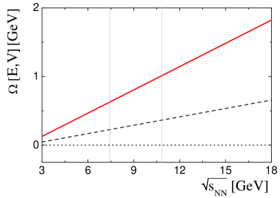
Figure 1: $\Omega[E,V]=\Delta[E,V]=\Sigma[E,V]=\omega^{*}[E]=\langle(\delta E)^{2}\rangle/\langle E\rangle$ as a function of $\sqrt{s_{NN}}$ in central Pb+Pb collisions at the CERN SPS energy range. See text for the numerical values of the model parameters and their $\sqrt{s_{NN}}$-dependence. The normalization factors $C_{\Delta}=C_{\Sigma}=\langle V\rangle$ are used. The solid, dashed, and dotted lines correspond to $\sqrt{\langle(\delta\varepsilon)^{2}\rangle}/\langle\varepsilon\rangle$ equal to 0.17, 0.13, and 0, respectively. The vertical lines indicate the beginning (the onset of deconfinement) and end (the softest point) of the mixed phase region, $\sqrt{s_{NN}}(OD)\cong 7.4$ GeV and $\sqrt{s_{NN}}(SP)\cong 10.8$ GeV, respectively.

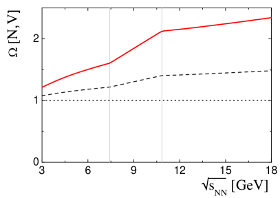
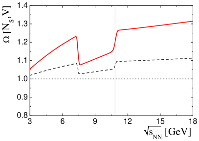
Figure 2: The same as in Fig. 1 but for $\Omega[N,V]=\Delta[N,V]=\Sigma[N,V]=\omega^{*}[N]$ (left) and $\Omega[N_{S},V]=\Delta[N_{S},V]=\Sigma[N_{S},V]=\omega^{*}[N_{s}]$ (right). The normalization factors $C_{\Delta}=C_{\Sigma}=\langle V\rangle$ are used.

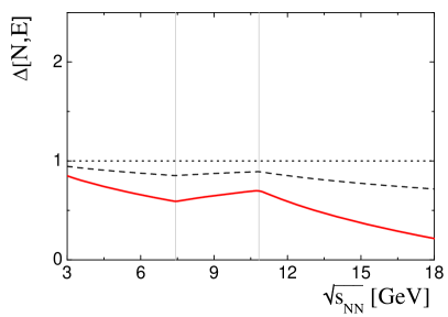
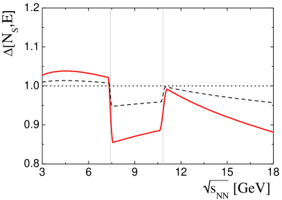
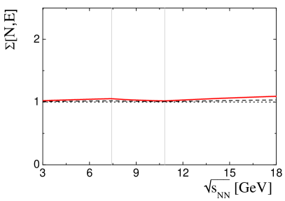
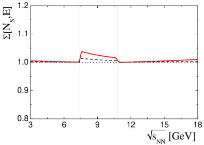
Figure 3: The same as in Figs. 1 and 2 but for $\Delta[N,E]$ and $\Sigma[N,E]$ (left), and $\Delta[N_{S},E]$ and $\Sigma[N_{S},E]$ (right). The normalization factors $C_{\Delta}=C_{\Sigma}=\langle E\rangle$ are used.

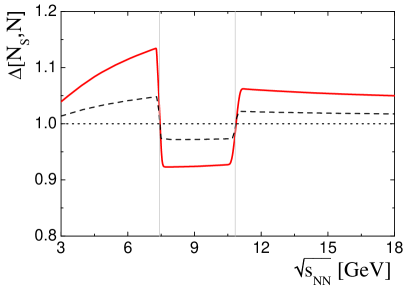
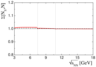
Figure 4: The same as in Figs. 1-3 but for $\Delta[N_{S},N]$ (left) and $\Sigma[N_{S},N]$ (right). The normalization factors $C_{\Delta}=\langle N\rangle-\langle N_{S}\rangle$ and $C_{\Sigma}=\langle N\rangle+\langle N_{S}\rangle$ are used.

The energy density fluctuations modify fluctuations of event properties like particle multiplicity and these modifications are dependent on the EoS and particle type. On the other hand the EoS and particle properties change significantly when crossing the phase transition region. Thus, one expects that the collision energy dependence of properly selected fluctuation measures may signal the transition region. The fluctuation measures which are sensitive to the EoS are plotted in Figs. 2-4 as functions of collision energy in the range which includes the phase transition region. Note that the $N$ and $N_{S}$ fluctuations for $\sqrt{\langle(\delta V)^{2}\rangle}/\langle V\rangle\leavevmode\nobreak\ =\leavevmode\nobreak\ 0$ and $\sqrt{\langle(\delta\varepsilon)^{2}\rangle}/\langle\varepsilon\rangle\leavevmode\nobreak\ =\leavevmode\nobreak\ 0$ are assumed to be Poissonian and uncorrelated.

17. The collision energy dependence of $\Omega[N,V]=\Delta[N,V]=\Sigma[N,V]=\omega^{*}[N]$ and $\Omega[N_{S},V]=\Delta[N_{S},V]=\Sigma[N_{S},V]=\omega^{*}[N_{S}]$ is shown in Fig. 2 for central Pb+Pb collisions at the CERN SPS energies. With $\sqrt{\langle(\delta\varepsilon)^{2}\rangle}/\langle\varepsilon\rangle$ decreasing to zero the results approach unity as expected in the IB-GCE. $\Delta$ and $\Sigma$ are equal to each other for pairs of quantities $[N,V]$ and $[N_{S},V]$. It results from the used approximations: $N$ and $N_{S}$ are uncorrelated in the fixed volume, $\langle N\rangle\sim V$ and $\langle N_{S}\rangle\sim V$, and $\langle(\delta V)^{2}\rangle/\langle V\rangle\cong 0$. The overall increasing trend of $\Omega[N,V]$ and $\Omega[N_{S},E]$ with $\sqrt{s_{NN}}$ seen in Fig. 2 is due to non-zero values of $\sqrt{\langle(\delta\varepsilon)^{2}\rangle}/\langle\varepsilon\rangle$. The modifications of this energy dependence are observed in the region of the phase transition. However, measurements of system volume (or quantity which is proportional to volume) are likely to be experimentally difficult or even impossible.

Figure 3 presents the fluctuation measures $\Delta[N,E]$ and $\Sigma[N,E]$ as well as $\Delta[N_{S},E]$ and $\Sigma[N_{S},E]$ as a function of collision energy. Similarly to the results presented in Fig. 2 the overall trend caused by the assumed energy density fluctuations is modified in the region of the phase transition. The most pronounced modification is observed for $\Delta[N_{S},E]$.

Finally, the collision energy dependence of $\Delta[N_{S},N]$ and $\Sigma[N_{S},N]$ is shown in Fig. 4. The normalization (8) is implied in this case. The most pronounced modification of the overall trend in the phase transition region is observed for $\Delta[N_{S},N]$, and a weak one for $\Sigma[N_{S},N]$.

18. In summary, predictions on the collision energy dependence of fluctuations of hadron production properties in central heavy ion collisions in the range of the phase transition are presented. They are based on the Statistical Model of the Early Stage and extend previously published results by predictions for the strongly intensive quantities. They are calculated for six pairs of event quantities:

$$[E,V],\leavevmode\nobreak\ \leavevmode\nobreak\ \leavevmode\nobreak\ [N,V],\leavevmode\nobreak\ \leavevmode\nobreak\ \leavevmode\nobreak\ [N_{S},V],\leavevmode\nobreak\ \leavevmode\nobreak\ \leavevmode\nobreak\ [N,E],\leavevmode\nobreak\ \leavevmode\nobreak\ \leavevmode\nobreak\ [N_{S},E],\leavevmode\nobreak\ \leavevmode\nobreak\ \leavevmode\nobreak\ [N_{S},N],$$ (13)

where $E$ and $V$ stand for the system energy and volume, whereas $N$ and $N_{S}$ for multiplicities of all and strange particles. In several considered cases the collision energy dependence is significantly modified in the phase transition region. The most pronounced change is seen for $\Delta[N_{S},N]$. This opens a possibility to observe signals of the onset of deconfinement in data on fluctuations of hadron production properties.