Nonlinear random optical waves: integrable turbulence, rogue waves and intermittency

Abstract

We examine the general question of statistical changes experienced by ensembles of nonlinear random waves propagating in systems ruled by integrable equations. In our study that enters within the framework of integrable turbulence, we specifically focus on optical fiber systems accurately described by the integrable one-dimensional nonlinear Schrödinger equation. We consider random complex fields having a gaussian statistics and an infinite extension at initial stage. We use numerical simulations with periodic boundary conditions and optical fiber experiments to investigate spectral and statistical changes experienced by nonlinear waves in focusing and in defocusing propagation regimes. As a result of nonlinear propagation, the power spectrum of the random wave broadens and takes exponential wings both in focusing and in defocusing regimes. Heavy-tailed deviations from gaussian statistics are observed in focusing regime while low-tailed deviations from gaussian statistics are observed in defocusing regime. After some transient evolution, the wave system is found to exhibit a statistically stationary state in which neither the probability density function of the wave field nor the spectrum change with the evolution variable. Separating fluctuations of small scale from fluctuations of large scale both in focusing and defocusing regime, we reveal the phenomenon of intermittency; i.e., small scales are characterized by large heavy-tailed deviations from Gaussian statistics, while the large ones are almost Gaussian.

I Introduction

The field of modern nonlinear physics has started with the pioneering work of Fermi and collaborators fermi1955studies who studied a chain of coupled anharmonic oscillators, now known as the FPU system, with the aim of understanding the effect of nonlinearities in the process of thermalization. Their unexpected results, i.e. the observation of a recurrent behavior instead of the phenomenon of thermalization, triggered the work by Zabusky and Kruskal zabusky1965 who performed numerical simulations of the Korteweg de Vries equation (KdV), i.e. the long wave approximation of the FPU system, and made the fundamental discovery of solitons; such discovery lead to the development of a new field in mathematical physics that deals with integrable systems with an infinite number of degrees of freedom. Some years after the discovery, Zakahrov and Shabat zakharov72 found that the Nonlinear Schrödinger equation (1D-NLSE) is an integrable partial differential equations and has multi-solution just like the KdV equation. The following years were characterized by the search of new integrable equations and the study of their mathematical properties and solutions.

In the late seventies and early eighties, besides solitons on a zero background, a new class of solutions of the 1D-NLSE were found kuznetsov1977solitons ; ma1979perturbed ; peregrine1983water ; akhmediev1985generation that describe the instability of a finite coherent background. Those solutions are sometimes named “breathers”: the classical Akhmediev akhmediev1985generation and the Peregrine peregrine1983water solutions breath just once in their life and they describe in toto the modulational instability process (also in its nonlinear stages). The Kuznetsov-Ma solution kuznetsov1977solitons ; ma1979perturbed is periodic in the evolution variable and the perturbation of the coherent state is never small.

The phenomenon of rogue waves (RW) in the ocean has been known to humans much before the discovery of integrability of partial differential equations; however, only in the last fifteen years a connection between those two fields has been made and it has been conjectured that the “breather” solutions of the focusing 1D-NLSE could be considered as rogue wave prototypes dysthe99 ; osborne00 . This idea has been rapidly picked up in different scientific communities kharif2009rogue ; Akhmediev:09 ; Akhmediev:09b ; Walczak:15 ; Dudley:14 ; Onorato:13 ; osborne2010nonlinear and a new field with fresh ideas and old equations has started. A first important step was the reproduction of the breather solutions of the 1D-NLSE in water wave tanks Chabchoub:11 ; Chabchoub:13 and in optical fibers Kibler:10 ; Kibler:12 ; Frisquet:13 . In order to generate these coherent structures in controlled lab experiments, very specific and carefully-designed coherent initial conditions have been considered. However, in nature such conditions are almost never encountered; wind generates ocean waves via a non trivial mechanism miles57 ; janssen91 and the resulting wave field appears as a superposition of random waves characterized by Fourier spectra with a small, but finite, spectral bandwidth. This suggests that the problem of rogue waves should be investigated from a statistical point of view Onorato:04 ; Erkintalo:10 ; Onorato:13 ; Walczak:15 . Indeed, one of the major question to be answered in the field of rogue waves concerns the determination of the probability density function (PDF) of the wave field for some given initial and boundary conditions. This is definitely not an easy task and, nowadays, given a nonlinear partial differential equation, there is no systematic theory that allows one to determine the PDF of the wave field.

The field of rogue waves has “belong” to oceanographers until the the pioneering experiments with optical fibers described in Solli:07 . Since then, optical rogue waves have been studied in various contexts such as supercontinuum generation in fibers Solli:07 ; Solli:08 ; Erkintalo:09 ; Kibler:09 ; Mussot:09 ; Dudley:14 , propagation in optical fiber described by the “pure” 1D-NLSE Walczak:15 or with higher order dispersion Taki:10 ; Conforti:15 , laser filamentation Kasparian:09 , passive cavities Montina:09 ; Conforti:15 , lasers Pisarchik:11 ; Bonatto:11 ; Lecaplain:12 ; Randoux:12 and Raman fiber amplifiers Hammani:08 .

From the general point of view and beyond the question of rogue waves, the field of nonlinear optics has then grown as a favorable laboratory to investigate both statistical properties of nonlinear random waves and hydrodynamic-like phenomena Babin:07 ; Turitsyn:10 ; Churkin:10b ; Michel:11 ; Turitsyna:13 ; Fatome:14 ; Picozzi:14 . Indeed, the field of incoherent dispersive waves resemble very much the classical field of fluid turbulence where, instead of waves, eddies interact with each other, giving birth to new eddies of different size. This mechanism is at the origin of the celebrated Kolmogorov cascade of the three-dimensional turbulence which is characterized by a constant flux of energy within the so called inertial range. A source and a sink of energy are required in order to maintain the cascade. Many years after such concept was developed, it was found that the cascade is intermittent, i.e. the statistical properties of the velocity field vary with the scales, becoming less Normal for smaller scales, see for example Frisch:95 for references. In the light of the paper Randoux:14 , this idea will be discussed in the present paper in the context of the dynamics of incoherent waves ruled by the integrable 1D-NLSE. Such equation provides a bridge between nonlinear optics and hydrodynamics, see chabchoub2015nonlinear for a one to one comparison. In particular, the focusing 1D-NLSE describes at leading order the physics of deep-water wave trains and it plays a central role in the study of rogue waves Onorato:01 ; Dudley:10 ; Onorato:13 ; Akhmediev:13 ; Dudley:14 . Moreover, the focusing 1D-NLSE is the simplest partial differential equation that describes the modulational instability phenomenon that is believed to be a fundamental mechanism for the formation of RW Onorato:04 ; Onorato:13 .

As mentioned, such waves emerge in the ocean from the interplay of incoherent waves in turbulent systems. The theoretical framework combining a statistical approach of random waves together with the property of integrability of the 1D-NLSE is known as integrable turbulence. This emerging field of research recently introduced by V. Zakharov relies on the analysis of complex phenomena found in nonlinear random waves systems described by an integrable equation Zakharov:09 ; Zakharov:13 ; Pelinovsky:13 ; Agafontsev:14c ; Randoux:14 ; Suret:11 . Strictly speaking, the word “turbulence” is not fully appropriate in the sense that the dynamics in Fourier space is not characterized by a constant flux of a conserved quantity because the system is Hamiltonian (no forcing and dissipation are included). For these integrable systems, given an initial condition, the spectrum generally relaxes to a statistically stationary state that in general is different from the standard thermal equilibrium characterized by the equipartition of energy. The prediction of the spectra of such final state and its statistical properties is the objective of the integrable turbulence field. In the weakly nonlinear regime Janssen:03 , starting with incoherent initial conditions in the 1D-NLSE, deviation from gaussian statistics has been predicted. In hydrodynamical numerical simulations performed with envelope equations and experiments made in water tanks, non gaussian statistics of the wave height has also been found to emerge from random initial conditions onorato2000occurrence ; Onorato:04 ; Onorato:05 .

While in the water wave context the NLSE is only a crude (but reasonable) approximation of the original equations of motion, the field of nonlinear fiber optics is a promising field for the investigation of integrable turbulence because optical tabletop “model experiments” accurately described by the 1D-NLSE can be performed Kibler:10 ; Kibler:12 ; Frisquet:13 ; Randoux:14 . Despite the numerous works devoted to optical RW, the generation of extreme events from purely stochastic initial conditions in focusing 1D-NLSE model experiments remains a crucial and open question Akhmediev:09b ; Akhmediev:13 ; Agafontsev:14c ; Dudley:14 .

In this paper, we review and extend a number of results recently obtained by the authors of this paper from optical fiber experiments Randoux:14 ; Walczak:15 in the anomalous and normal dispersion regime. The dynamics of the waves in the considered fiber is described with high accuracy by the focusing and defocusing 1D-NLSE. In the focusing regime, the idea is to implement optical fiber experiments conceptually analogous to the water tank experiment described in Onorato:04 where waves with a finite spectral bandwidth and random phases are generated at one end of the tank and the evolution of the statistical properties of the wave field is followed along the flume. Using an original setup to overcome bandwidth limitations of usual detectors, we evidence strong distortions of the statistics of nonlinear random light characterizing the occurrence of optical rogue waves in integrable turbulence.

In the defocusing regime, modulational instability is not possible and the evolution of incoherent waves does not lead to the formation of rogue waves. The statistics of wave intensity, initially following the central limit theorem, changes along the fiber resulting in a decrease of the tails of the PDF. This implies that the probability of finding a rogue wave is lower than the one described by linear theory. Implementing an optical filtering technique, we also report on the statistics of intensity of light fluctuations on different scales and we observe that the PDF of the wave intensity show tails that strongly depend on the scales. This reveals the phenomenon of intermittency, previously mentioned, that is similar to the one reported in several other wave systems, though fundamentally far from being described by an integrable wave equation. We also report new and original experimental results for partially coherent waves having a broad spectrum. We demonstrate in particular the emergence of strongly non gaussian statistics with low tailed PDF in the defocusing regime.

The paper is organized as follows: numerical simulations of focusing and defocusing 1D-NLSE are first considered and described in Sec. II. Optical fiber experiments designed to investigate changes in the statistics of random light fields and showing results in agreement with simulations are presented in Sec. III. In Sec. IV, we show that the integrable wave system under consideration exhibit a phenomenon of intermittency both in focusing and defocusing regime. In Sec. V, we summarize our work and we discuss open questions about integrable turbulence.

II Spatio-temporal, spectral and statistical features arising from nonlinear propagation of random waves in systems ruled by the integrable 1D-NLSE

II.1 General framework and description of the random initial condition

Our study enters within the general framework of the integrable 1D-NLSE:

$$i\psi_{t}+\psi_{xx}+2\,\sigma\,|\psi|^{2}\,\psi=0$$ (1)

where $\psi(x,t)$ is the complex wave envelope. The parameter $\sigma$ determines the focusing ($\sigma=+1$) or defocusing ($\sigma=-1$) nature of the propagation regime. In nonlinear fiber optics, it is relatively easy to explore each of the two propagation regimes just by changing either the fiber or the wavelength of light Agrawal . Eq. (1) conserves the energy (or Hamiltonian) $H=H_{L}+H_{NL}$ that has a nonlinear contribution $H_{NL}=-\sigma\int|\psi(x,t)|^{4}dx$ and a linear (kinetic) contribution $H_{L}=\int k^{2}|\widehat{\psi}(k,t)|^{2}dk$, the Fourier transform being defined as $\widehat{\psi}(k,t)=1/\sqrt{2\pi}\int\psi_{0}(x,t)e^{-ikx}dx$. Eq. (1) also conserves the number of particules (or power) $N=\int|\psi(x,t)|^{2}dx$ and the momentum $P=\int k|\psi(k,t)|^{2}dk$.

In our paper, the initial conditions that are used are non-decaying random complex fields. We examine a situation that is very different from the problem of the Fraunhoffer diffraction of nonlinear spatially incoherent waves already considered in ref. Bass:87 ; Bromberg:10 ; Derevyanko:08 ; Derevyanko:12 . In these papers, the nonlinear propagation of a speckle pattern of limited and finite spatial extension is studied in focusing and defocusing media. On the other hand we consider here continuous random waves of infinite spatial extension. This corresponds for instance to an experimental situation in which a partially coherent and continuous (i.e. not pulsed) light source of high power is launched inside a single-mode optical fiber Randoux:14 ; Walczak:15 . In numerical simulations, the random waves are confined in a box of size $L$ and periodic boundary conditions ($\psi(x=0,t)=\psi(x=L,t)$) are used to describe their time evolution Nazarenko .

The random complex field $\psi(x,t=0)=\psi_{0}(x)$ used as initial condition in this paper is made from a discrete sum of Fourier components :

$$\psi(x,t=0)=\psi_{0}(x)=\sum\limits_{n}\widehat{\psi_{0n}}e^{ink_{0}x}.$$ (2)

with $\widehat{\psi_{0n}}=1/L\int_{0}^{L}\psi_{0}(x)e^{-ink_{0}x}dx$ and $k_{0}=2\pi/L$. The Fourier modes $\widehat{\psi_{0n}}=|\widehat{\psi_{0n}}|e^{i\phi_{0n}}$ are complex variables. In the random phase and amplitude (RPA) model, generation of a random initial complex field is achieved by taking $|\widehat{\psi}_{0n}|$ and $\phi_{0n}$ as randomly-distributed variables Nazarenko . Here, we will mainly use the so-called random phase (RP) model in which only the phases $\phi_{0n}$ of the Fourier modes are considered as being random Nazarenko . In this model, the phase of each Fourier mode is randomly and uniformly distributed between $-\pi$ and $\pi$. Moreover, the phases of separate Fourier modes are not correlated so that $<e^{i\phi_{0n}}e^{i\phi_{0m}}>=\delta_{nm}$. In the previous expression, the brackets represent an average operation made over an ensemble of many realizations of the random process. $\delta_{nm}$ is the Kronecker symbol defined by $\delta_{nm}=1$ if $n=m$ and $\delta_{nm}=0$ if $n\neq m$.

With the assumptions of the RP model above described, the statistics of the initial field is homogeneous, which means that all statistical moments of the initial complex field $\psi_{0}(x)$ do not depend on $x$ Picozzi:07 ; Picozzi:14 . The power spectrum $n_{0}(k_{n})$ of the random field $\psi_{0}(x)$ then reads as :

$$<\widehat{\psi_{0n}}\widehat{\psi_{0m}}>=n_{0n}\,\delta_{nm}=n_{0}(k_{n}).$$ (3)

with $k_{n}=n\,k_{0}$. In the limit where $L\rightarrow\infty$, the frequency separation between two neighboring frequency components $k_{n}$ and $k_{n+1}$ tends to zero and the discrete spectrum $n_{0}(k_{n})$ becomes a continuous spectrum $n_{0}(k)$.

The RP model is often used in the contexts of hydrodynamics where the power spectrum $n_{0}(k)$ is given by the so-called JONSWAP spectrum Islas:05 ; Onorato:01 It has also been used in optics where simple gaussian or sech profiles are often used for the function $n_{0}(k)$ Suret:11 ; Randoux:14 ; Walczak:15 .

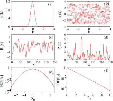
Figure 1: (a) Gaussian power spectrum $n_{0}(k)$ of the initial condition such as defined by Eq. (4) ( $\Delta k=0.5$, $n_{0}=1.129$). (b) Spectral distribution of the phases $\phi_{0}(k)$ of the Fourier modes used to compute the random initial field $\psi_{0}(x)$. (c) Real part $R_{0}(x)=\Re{(\psi_{0}(x))}$ and (d) power $P_{0}(x)=|\psi_{0}(x)|^{2}$ of the random field computed from spectra shown in (a), (b). (e) PDF of $R_{0}(x)$ and (f) PDF of $P_{0}(x)$ showing that the initial condition has a gaussian statistics.

In this Section, we consider a random complex initial field having a gaussian optical power spectrum that reads

$$n_{0}(k)=n_{0}\,\exp\left[-\left(\frac{k^{2}}{\Delta k^{2}}\right)\right]$$ (4)

where $\Delta k$ is the half width at $1/e$ of the power spectrum. Fig. 1 shows a typical example of a partially coherent complex field generated using the RP model and a power spectrum given by Eq. (4). Fig. 1(b) shows that the values of the spectral phases $\phi_{0}(k)$ are randomly distributed between $-\pi$ and $\pi$. Fig. 1(c) shows the random evolution of the real part $R_{0}(x)=\Re{(\psi_{0}(x))}$ of the initial field that is computed from the spectra shown in Fig. 1(a) and 1(b). We do not present here the evolution of the imaginary part $I_{0}(x)=\Im{(\psi_{0}(x))}$ of the initial field because it is qualitatively very comparable to what is shown in Fig. 1(c). However it is important to notice that the RP model produces a random field having real and imaginary parts that are statistically independent, i.e. $<R_{0}(x)I_{0}(x)>=0\,\,\,\forall\,x$. The spatial evolution of the power $P_{0}(x)=|\psi_{0}(x)|^{2}=R_{0}^{2}(x)+I_{0}^{2}(x)$ of the random initial field is shown in Fig. 1(d). Note that the numerical values of the parameters $n_{0}$ and $\Delta k$ have been chosen in such a way that the number of particules $N=1/L\int_{0}^{L}|\psi(x,t)|^{2}dx$ is equal to unity.

As previously described, the random complex field $\psi_{0}(x)$ used as initial condition is produced from the linear superposition of a large number of independent Fourier modes having randomly distributed phases. As stated by the central limit theorem, the statistics of the random process produced from such a superposition follows the normal law. The RP model thus produces a complex field having quadratures that are statistically independent and that have the same gaussian statistics. It is straightforward to prove that the statistics of power fluctuations $P_{0}$ follows the exponential distribution Mandel_wolf ; Agafontsev:14c . Note that the PDF for the fluctuations of the amplitude $A_{0}(x)=|\psi_{0}(x)|$ is given by the Rayleigh distribution defined by $PDF[A_{0}/<A_{0}>]=A_{0}/<A_{0}>\,.\,exp(-A_{0}/<A_{0}>)$ Mandel_wolf ; Agafontsev:14c

In order to illustrate these statistical features from numerical simulations, we have performed the analysis of the statistical properties of the complex field generated from the RP model by producing an ensemble of $10^{4}$ realizations of the random initial field. From this ensemble, it is in particular possible to compute the PDF for the fluctuations of $R_{0}(x)=\Re{(\psi_{0}(x))}$ and of $P_{0}(x)=|\psi_{0}(x)|^{2}$. Fig. 1(e) shows that the PDF of $R_{0}(x)/<R_{0}(x)>$ is gaussian. The PDF of the normalized imaginary part $I_{0}(x)/<I_{0}(x)>$ of the complex field is not shown here but it is rigorously identical to the PDF of $R_{0}(x)/<R_{0}(x)>$. As it is illustrated in Fig. 1(f), the PDF of the power is given by the exponential distribution, i.e. $PDF[P_{0}/<P_{0}>]=exp(-P_{0}/<P_{0}>)$.

II.2 Focusing regime

In this Section, we consider the focusing regime ($\sigma=+1$) and we use numerical simulations of Eq. (1) to investigate the propagation of a partially coherent wave generated at $t=0$ by the random complex field described in Sec. II.1. We will consider the spatio-temporal dynamics of the partially coherent wave and we will also discuss spectral and statistical changes occurring in time.

Our numerical simulations have been performed by using a pseudo-spectral method working with a step-adaptative algorithm permitting to reach a specified level of numerical accuracy. The numerical simulations are performed by using a box of size $L=257.36$ that has been discretized by using $4096$ points. Statistical properties of the random wave are computed from an ensemble of $10^{4}$ realizations of the random initial condition.

Fig. 2(a) shows the spatio-temporal evolution of the partially-coherent wave seeded by a random initial field having properties that are described in Sec.II.1 and that are synthesized in Fig. 1. At the initial stage of the nonlinear evolution ($t\sim 0$), the power $|\psi(x,t)|^{2}$ of the wave is slowly and randomly modulated. The spatial scale of the fluctuations of $|\psi(x,t)|^{2}$ at $t\sim 0$ is determined by $\Delta k$ and it is typically around $10$ in the simulations shown in Fig. 2 (see also Fig.1(d)). Numerical simulations show that series of peaks emerge from the random initial condition. The density of these peaks is higher is those regions of space where the complex field exhibits high peak power fluctuations at the initial time $t=0$, see e. g. the region where $x\in[-50,-40]$ in Fig. 2 and in Fig. 3(a),(c),(e). While the localized peaks shown in Fig. 2(a) drift with small velocities in the $(x,t)$ plane, their peak power increases with time. This increase of the peak power of the localized structures goes simultaneously with a reduction of their spatial width. The typical spatial scale of the power fluctuations evolves from a value of $\sim 10$ at initial stage ($t=0$) to the healing length of $\sim 1$ at long evolution time ($t>10$) (see Fig. 3(a) , (c), (e)).

A clear signature of the change in the fluctuation scale can be observed in the Fourier space. As shown in Fig. 3(b), 3(d) and 3(f), the power spectrum $|\widehat{\psi}(k,t)|^{2}$ of the random wave is indeed found to significantly broaden with time. Let us emphasize that the power spectrum of the wave broadens while always keeping exponentially decaying wings.

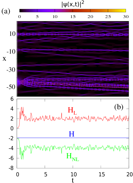
Figure 2: Numerical simulations of Eq. (1) in focusing regime ($\sigma=+1$). (a) Spatio-temporal evolution of the power $|\psi(x,t)|^{2}$ of the wave while starting from the random complex field having a gaussian power spectrum and a gaussian statistics, see Fig. 1. (b) Corresponding time evolution of linear (kinetic) energy $H_{L}$ and of nonlinear energy $H_{NL}$.

The evolution of the typical space scales and peak powers of the random fluctuations that is described above goes together with a process of energy balance between linear and nonlinear effects. Fig. 2(b) shows the evolutions in time of the linear (kinetic) energy $H_{L}$ and of the nonlinear energy $H_{NL}$ that are associated with the spatio-temporal evolution plotted in Fig. 2(a). The wave system is initially placed in a highly nonlinear regime in which the nonlinear energy is one order of magnitude greater than the linear energy ($|H_{NL}|\simeq 10|H_{L}|$). As a result of nonlinear propagation, linear and nonlinear effects come into balance and after a short transient evolution, the wave system reaches a state in which linear and nonlinear energies have the same order of magnitude ($|H_{NL}|\simeq 2|H_{L}|$, see Fig. 2(b) ).

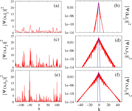
Figure 3: Numerical simulations of Eq. (1) in focusing regime ($\sigma=+1$). Spatial evolution of the power $|\psi(x,t)|^{2}$ of the random wave at times (a) $t_{1}=0.24$, (c) $t_{1}=2.44$ , (e) $t_{1}=16.04$. Power spectra (red lines) $|\psi(k,t)|^{2}$ of the random wave at times (b) $t_{1}=0.24$, (d) $t_{1}=2.44$ , (f) $t_{1}=16.04$. The spectra plotted in blue lines represent the gaussian power spectrum of the random initial complex field defined by Eq. (3) and Eq. (4).

It is interesting to compare the spatio-temporal evolution shown in Fig. 2(a) with the one shown in Fig. 2(a) of ref. Toenger:15 . In ref. Toenger:15 , the authors study the nonlinear evolution in space and time of a condensate perturbated by a small noise, i. e. $\psi_{0}(x)=1+\eta(x)$ where $|\eta(x)|<<1$ is a small noise with broad spectrum. As shown in Fig. 2(a) of ref. Toenger:15 , the fact that there is only a weak random modulation of the initial condition gives rise to a spatiotemporal diagram in which localized structures are distributed in space and time in a way that is more regular than the random pattern shown in Fig. 2(a) of this paper. Starting from our initial condition with a broad gaussian spectrum, there are some wide regions of space in which no localized structures are observable while there are some other regions of space including many localized structures. As shown in ref. Walczak:15 , the localized structures emerging from a complex field having initially a gaussian statistics can be locally fitted by some analytical functions corresponding to solitons on finite background, such as e. g. the Peregrine soliton. Fitting procedures implemented in the numerical work presented in ref. Toenger:15 have shown that many solitons on finite background can be also found while seeding the wave system from a condensate perturbated by a small noise.

Despite localized structures looking like solitons on finite background can be observed while starting from those two different random initial conditions, significantly different statistical features are observed at long evolution time. It has been shown in ref. Agafontsev:14c that gaussian statistics emerges from the nonlinear evolution of the noisy condensate. As shown in Fig.4(a), heavy-tailed deviations from gaussianity are contrarily found to emerge from a random complex field having initially a gaussian statistics Walczak:15 . It is an open question to understand how the interplay among localized structures does not produce the same statistics at long evolution time while starting from different noisy initial conditions.

Rational solutions of the 1D-NLSE such as Akhmediev breathers are considered as prototype of rogue waves Akhmediev:09 ; Akhmediev:09b . These coherent structures have been generated in optical fiber experiments Kibler:10 ; Kibler:12 and in hydrodynamical experiments Chabchoub:11 . The interaction of solitons Pelinovsky and the collision of breathers have been studied theoretically and experimentally Frisquet:13 . Our work points out the relevance of these works and the need to extend it in the context of random nonlinear waves. In particular, it is an open question to understand the mechanisms of the emergence of coherent structures from the two different initial conditions, i.e. the plane wave with small noise on one hand and the random wave computed from the RP model on the other hand.

Fig. 4 shows the time evolution of the PDF of $|\psi(x,t)|^{2}$. The nonlinear random field has a statistical evolution in which the PDF of power fluctuations continuously moves from the exponential distribution (plotted in red line in Fig. 4) to the heavy-tailed distribution plotted in magenta line in Fig. 4. For $t>10$, the wave system reaches a statistical stationary state in which the PDF no longer changes with time Walczak:15 . This statistical stationary state is determined by the interaction of coherent nonlinear structures such as for instance Akhmediev breathers, Kuznetsov-Ma solitons and also linear dispersive radiation Pelinovsky:13 ; Efimov:05 ; Bohm:06 . It is now an open question to determine the mechanisms in integrable turbulence that lead to the establishment of a stationary state in which statistical properties of the wave system do not change in time. Tools from the inverse scattering theory could be used to investigate this question of fundamental importance Bass:87 ; Gennadyprl:05 ; Bohm:06 ; Derevyanko:08 ; Derevyanko:12

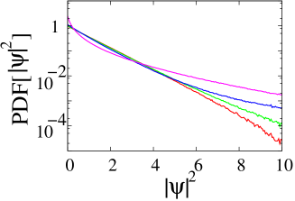
Figure 4: Numerical simulations of Eq. (1) in focusing regime ($\sigma=+1$). PDF of the power $|\psi(x,t)|^{2}$ at time $t=0$ (red line), $t=0.2$ (green line), $t=0.4$ (blue line), $t=10$ and $t^{*}=20$ (magenta line). The PDF is stationary from $t\sim 10$, i.e. the PDF plotted in magenta line does not change with time for $t>10$.

II.3 Defocusing regime

In this Section, we consider the defocusing regime ($\sigma=-1$) and we use numerical simulations of Eq. (1) to investigate the propagation of a partially coherent wave generated at $t=0$ by a random complex field identical to the one used in Sec. II.2.

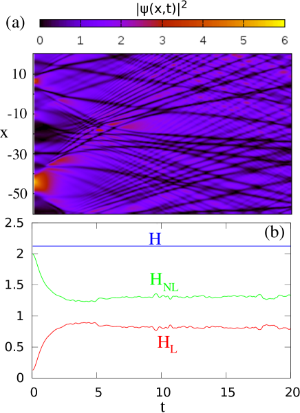
Figure 5: Numerical simulations of Eq. (1) in defocusing regime ($\sigma=-1$). (a) Spatio-temporal evolution of the power $|\psi(x,t)|^{2}$ of the wave while starting from the random complex field having a gaussian power spectrum and a gaussian statistics, see Fig. 1. (b) Corresponding time evolution of linear (kinetic) energy $H_{L}$ and of nonlinear energy $H_{NL}$.

Fig. 5(a) shows the spatio-temporal evolution of the partially-coherent wave seeded by a random initial field identical to the one used in Fig. 2(a). Spatiotemporal features emerging from the nonlinear propagation in defocusing regime drastically contrast with those found in the focusing regime. Instead of bright localized structures, we now observe the emergence of dark localized structures propagating at various speeds in the $(x,t)$ plane. Fig. 6(a) and 6(b) show that the initial stage of nonlinear evolution is now characterized by a fast decay of the peaks of highest intensities, see e. g. the region where $x\in[-50,-40]$. During the initial evolution of the random wave, the leading and trailing edges of peaks of highest intensities strongly sharpen. This leads to some gradient catastrophes which are regularized by the generation of dispersive shock waves (DSWs) Fatome:14 ; Conforti:13 ; Conforti:14 ; Moro:14 ; Gennady:05 . As in the focusing case, the typical spatial scale of the random fluctuations decreases from $\sim 10$ at the initial stage ($t=0$) to the healing length of $\sim 1$ at long evolution time ($t>10$). The stochastic evolution shown in Fig. 6(c) is determined by the interaction of nonlinear coherent structures such as dark solitons or DSWs and of linear radiation.

Fig. 6(b), 6(d) and 6(f) show that nonlinear propagation in defocusing regime induces a spectral broadening of the random wave. This spectral broadening phenomenon is quantitatively less pronounced than the one observed in the focusing regime, see Fig. 3(b), 3(d), 3(f). However the power spectrum of the wave broadens while always keeping exponentially decaying wings, as in the focusing regime.

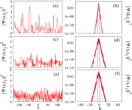
Figure 6: Numerical simulations of Eq. (1) in defocusing regime ($\sigma=-1$). Spatial evolution of the power $|\psi(x,t)|^{2}$ of the random wave at times (a) $t_{1}=0.24$, (c) $t_{1}=2.44$ , (e) $t_{1}=16.04$. Power spectra (red lines) $|\psi(k,t)|^{2}$ of the random wave at times (b) $t_{1}=0.24$, (d) $t_{1}=2.44$ , (f) $t_{1}=16.04$. The spectra plotted in blue lines represent the gaussian power spectrum of the random initial complex field defined by Eq. (3) and Eq. (4).

The spatiotemporal evolution shown in Fig. 5(a) and in Fig. 6(a), (c), (e) goes together with a process of energy balance between linear and nonlinear effects. Fig. 5(b) shows the time evolutions of the linear (kinetic) energy $H_{L}$ and of the nonlinear energy $H_{NL}$ that are associated with the spatio-temporal evolution plotted in Fig. 5(a). The wave system is initially placed in a highly nonlinear regime in which the nonlinear energy is one order of magnitude greater than the linear energy ($H_{NL}\sim 10H_{L}$). As in the focusing regime, linear and nonlinear effects come into balance and after a short transient evolution, the wave system reaches a state in which $H_{NL}$ and $H_{L}$ have the same order of magnitude, see Fig. 5(b).

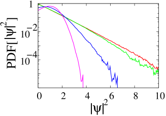
Figure 7: Numerical simulations of Eq. (1) in defocusing regime ($\sigma=-1$). PDF of the power $|\psi(x,t)|^{2}$ at time $t=0$ (red line), $t=0.2$ (green line), $t=1$ (blue line), $t=10$ and $t^{*}=20$ (magenta line). The PDF is stationary from $t\sim 10$, i.e. the PDF plotted in magenta line does not change with time for $t>10$.

In the defocusing regime, the nonlinear random field has a statistical evolution in which the PDF of power fluctuations continuously moves from the exponential distribution (plotted in red line in Fig. 7) to the low-tailed distribution plotted in magenta line in Fig. 7. As in the focusing regime, the wave system exhibits a statistical stationary state and the PDF computed at $t=10$ (magenta line in Fig. 7) does not change anymore with time Randoux:14 . This statistical stationary state is determined by the interaction of coherent nonlinear structures such as for instance dark solitons, dispersive shock waves and also linear radiation. As for the focusing regime, it is an open question to determine the mechanisms in integrable turbulence that lead to the establishment of a stationary state in which statistical properties of the wave system do not change in time. Tools of the inverse scattering transform could be of interest for the investigation of this question Fratolocchi:08 .

III Optical fiber experiments in focusing and in defocusing propagation regimes

Optical fiber experiments provide versatile and powerful tabletop laboratory to investigate the complex dynamics of 1DNLSE, hydrodynamic-like phenomena and the statistical properties of nonlinear random waves Babin:07 ; Turitsyn:10 ; Gorbunov:14 ; Turitsyna:13 ; Chabchoub:13 ; Fatome:14 ; Picozzi:14 ; Solli:07 ; Dudley:14 .

One of the most critical constraint of these experiments is the finite spectral bandwidth of usual detectors. The typical response time of the fastest detector and oscilloscope is several tens of picoseconds. On the other hand, with the usual parameters of standard experiments using optical fibers, the typical “healing time” scale characterizing the equilibrium between the nonlinearity and the dispersion is around one picosecond Walczak:15 . For this reason, the picosecond is also the order of magnitude of the time scale associated to the power fluctuations of partially coherent fiber lasers Babin:07 ; Turitsyn:10 ; Walczak:15b .

As a consequence spectral filters are therefore often used to reveal extreme events in time-domain experiments Solli:07 ; Erkintalo:09 ; Randoux:12 ; Randoux:14 . In the case of pulsed experiments, it is possible to evidence shot-to-shot spectrum fluctuations with a dispersive Fourier transform measurement Solli:07 ; Jalali:10 ; Wetzel:12 ; Goda:13 . To the best of our knowledge, up to our recent works Walczak:15 ; Walczak:15b , the accurate and well-calibrated measurement of the PDF characterizing temporal fluctuations of the power of random light with time scale of the order of picosecond had never been performed.

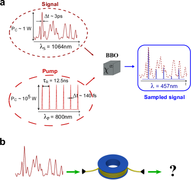
Figure 8: Experimental measurement of the statistics of random light a. Principle. Optical sampling of the partially-coherent wave fluctuating with time (the signal) is achieved from sum frequency generation in a second order ($\chi^{(2)}$) crystal. Blue pulses are generated at $\lambda=457$nm from the interaction of the signal with periodic femtosecond pump pulses inside a $\chi^{(2)}$ crystal. PDF is computed from the peak powers of the blue pulses. b. Nonlinear propagation in optical fiber The initial partially coherent light is launched inside a single mode optical fiber (either in the focusing (fiber 1) or defocusing (fiber 2) regime of dispersion. The statistics and the spectrum is measured before and after the propagation in the fiber.

We have developed an original setup based on asynchronous optical sampling (OS) which allows the precise measurement of statistics of random light rapidly fluctuating with time (see Fig. 8).

The “random light” under investigation is a partially coherent wave and it is called the “signal”. The signal is optically sampled with 140fs-pulses and the PDF is computed from the samples. The optical sampling is obtained from the second order nonlinearity $\chi^{(2)}$ in a BBO crystal. The sum-frequency generation (SFG) between the signal at $\lambda_{S}=1064$nm and short “pump” pulses having a central wavelength $\lambda_{P}=800$nm provide samples of the signal at a wavelength $\lambda=457$nm.

In our experiments, the linearly polarized partially coherent wave is emitted by a “continuous” wave (cw) Ytterbium fiber laser at $\lambda_{S}=1064$nm. This cw laser emits numerous (typically $10^{4}$) uncorrelated longitudinal modes. The reader can refer to Walczak:15 for the details of the experimental setup and of the statistics measurement procedure.

In this paper we present results obtained with two different fibers (fiber 1 and 2) having opposite sign of the group velocity dispersion at the wavelength of the signal $\lambda_{S}=1064$nm. The fiber 1 is a 15m-long highly nonlinear photonic crystal fiber (provided by Draka France company) with a nonlinear third order coefficient $\gamma\simeq 50$W^-1km^-1 and a group velocity dispersion coefficient $\beta_{2}\simeq-20ps^{2}/km$. The fiber 2 is a 100m-long polarization maintaining fiber with a nonlinear third order coefficient $\gamma\simeq 6$W^-1km^-1 and a group velocity dispersion coefficient $\beta_{2}\simeq+20ps^{2}/km$. We launch a mean power $<P>=0.6$W in the experiments performed with the fiber 1 (focusing case) and a mean power $<P>=4.$W in the experiments performed with the fiber 2 (defocusing case). Note that the results obtained with the fiber 1 have been presented in detail in Walczak:15 whereas the results obtained with the fiber 2 are new.

We first measure the PDF at the output of the laser. In all experiments presented in this letter, the mean output power of the Ytterbium laser is fixed at $\langle P\rangle=10$W. At this operating point, the statistics of the partially coherent wave follows the normal law. Indeed, as plotted in red in Figs. 9.c and 9.d, the PDF of the normalized power $P/\langle P\rangle$ is very close to the exponential function. Assuming that the real part and the imaginary parts are statistically independent, this exponential distribution of power corresponds to a gaussian statistics of the field. It is important to note that the dashed black lines in Figs. 9.c and 9.d are not a fitted exponential function but represent the exact normalized $PDF[P/\langle P\rangle]=\exp(-P/\langle P\rangle)$. To the best of our knowledge, PDF of so rapidly fluctuating optical signals has never been quantitatively compared to the normalized exponential distribution.

We use the output of the laser as a random source and we launch the partially coherent signal into optical fibers 1 and 2. Experiments have been carefully designed to be very well described by the 1D-NLSE. In particular, the signal wavelength $\lambda_{s}=1064$nm is far from the zero-dispersion wavelength ($\lambda_{0}$$\simeq 970$nm for the fiber 1 and $\lambda_{0}>1300$nm for the fiber 2). Moreover the optical spectral widths (see Figs. 9.a and 9.b) remain sufficiently narrow to neglect stimulated Raman scattering (SRS) and high-order dispersion effects. The linear losses experienced by optical fields in single pass in the fibers are neglictible. These total losses are around $0.3\%$ in the fiber 1 and around around $2.5\%$ in the fiber 2.

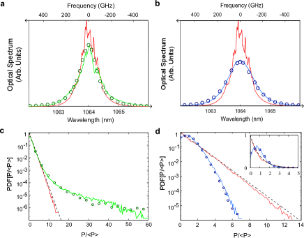
Figure 9: Experiments. a,b : Optical spectra. Input spectrum (red line). Spectrum at the output of fiber 1 (green line) and fiber 2 (blue line). The circles represents optical spectra computed from numerical simulation of 1D-NLSE. c, d : PDF of normalized optical power $P/\langle P\rangle$ plotted in logarithmic scale. Normalized exponential distribution $PDF[P/<P>]=\exp(-P/<P>)$ (black dashed line). PDF of the input random light (red line). PDF of the light at the output of the fiber 1 (green solid line) and at the output of the fiber 2 (blue solid line). The dashed lines represent the PDF computed from numerical simulation of 1D-NLSE with the parameters of the experiments. The inset represents the same PDF in linear scale.

Despite the broadening of the optical spectrum is of nearly the same importance in focusing and in defocusing regimes (see Figs. 9.a and 9.b) our experiments reveal that the distortions of the statistics of the random waves strongly depend on the sign of the group velocity dispersion coefficient.

The experiments performed in the focusing regime (fiber 1) reveal the occurrence of numerous extreme events (RW) (see green curve in Fig. 9.c). The comparison between the initial PDF (see red line in Fig. 9.c) and the output PDF (see green curve 9.c) shows an impressive change in the statistical distribution of optical power. The initial field follows the normal law and its PDF is an exponential function whereas the output PDF of optical power exhibits a strong heavy-tail.

On the other hand, the PDF experimentally measured at the output of fiber 2 in the defocusing regime exhibits a very low tail (see Fig. 9.d). Light fluctuations of a high power are found with a probability that has been strongly reduced as compared to the normal law. Moreover, contrary to the initial exponential distribution, the most probable value for the power is not the zero value (see inset of Fig. 9.d) ).

Numerical simulations show that experiments presented above are very well described by the integrable 1D-NLSE. The initial conditions are computed from the random phase assumption as in the section II.1. We have performed Monte Carlo simulations with ensemble average over thousands of realizations. We integrate the 1D-NLSE with experimental parameters :

$$i\frac{\partial\psi}{\partial z}=\frac{\beta_{2}}{2}\frac{\partial^{2}\psi}{\partial t^{2}}-\gamma|\psi|^{2}\psi$$ (5)

where $\beta_{2}$ is the group velocity dispersion coefficient and $\gamma$ is the effective Kerr coefficient. Optical spectra and PDFs computed from the numerical integration of the 1D-NLSE are in quantitative agreement with experiments both in the focusing and in the defocusing cases (see dashed green and blue lines in Fig. 9).

Moreover, the numerical simulations show that integrable turbulence is characterized by a statistical stationary state both in focusing and defocusing regime (see Fig. 10). In particular, the average of the nonlinear and linear parts of the Hamiltonian ($\langle H_{NL}\rangle$ and $\langle H_{L}\rangle$) evolves to constant values (see Figs. 10.a and 10.b). Note that we represent here the average of $H_{NL}$ and $H_{L}$ over hundreds of realizations whereas the values of $H_{NL}$ and $H_{L}$ computed on only one realization are plotted in section II.

Fig. 10.c represents PDFs computed from numerical simulations for different lengths of propagation in the focusing regime of dispersion. The red line is the PDF at $z=0$m, the green line is the PDF at $z=15m$ corresponding to the experiments (see Fig. 9.c) and the black line corresponds at the stationary PDF (computed at $z=500$m). Fig. 10.d represents PDFs computed from numerical simulations for different lengths of propagation in the defocusing regime of dispersion. The red line is the PDF at $z=0$m, the blue line is the PDF at $z=100m$ corresponding to the experiments (see Fig. 9.d) and the black line corresponds to the stationary PDF (computed at $z=500$m).

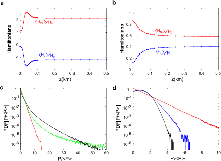
Figure 10: Numerical Simulations. a and b : evolution of the average of the nonlinear $H_{NL}$ and linear $H_{L}$ Hamiltonians in the focusing (a) and defocusing (b) cases. $H_{NL}$ and $H_{L}$ are normalized to the value of the Hamiltonian (constant of motion) $H=H_{NL}+H_{L}$ before the averaging over hundreds of realizations. c. PDFs computed at different $z$ in the focusing case. $z=0$m (red line), $z=15m$ (green line, identical to dashed green line in Fig. 9.c) and $z=100m$ (stationary PDF). d. PDFs computed at different $z$ in the defocusing case. $z=0$m (red line), $z=100m$ (blue line, identical to dashed blue line in Fig. 9.d) and $z=500m$ (stationary PDF).

Note that comparable deviations from gaussian statistics have been reported in 1D “spatial experiments” in which the transverse intensity profile of optical beams randomly fluctuates in space Bromberg:10 . In these spatial experiments performed in focusing and defocusing regime, the speckle fields are localized and random waves decay to zero at infinity Bromberg:10 ; Derevyanko:12 . IST with usual zero-boundary conditions has been used in ref. Derevyanko:12 to describe these experiments. In the long-term evolution of the wave system with zero boundary conditions, solitons separate from dispersive waves in the focusing regime. In the defocusing regime, only dispersive waves persist at long evolution time.

On the contrary, our experiments and numerical simulations are made with non-zero boundary conditions and with non-localized random waves. This widens the perspectives of experimental integrable turbulence studies. With random waves having an infinite spatial extension, solitons and dispersive waves never separate from each other and they always interact. Moreover breathers and solitons on finite background can emerge from nonlinear interaction in the focusing regime. In the defocusing case, the fact that the random field does not decay at infinity means that dark solitons can be sustained and interact all-together with dispersive waves at any time (any value of $z$ in our fiber experiments).

As a conclusion of Sec. III, we have experimentally studied the evolution of the statistics of random waves whose propagation is very well described by 1D-NLSE both in focusing and defocusing case.

In the defocusing case, we have experimentally and numerically demonstrated that the probability of occurrence of large waves decreases as a result of nonlinear propagation.

In the focusing case, we have evidenced the statistical emergence of RW from nonlinear propagation of random light. In Walczak:15 , we have also shown that solitons on finite background such as Akhmediev breathers, Peregrine solitons or Kuznetsov-Ma solitons having a short duration and a high power seem to emerge on the top of the highest fluctuations. This strengthens the idea that the emergence of deterministic solutions of 1D-NLSE such as Akhmediev breathers in nonlinear random fields is a major mechanism for the formation of rogue waves Akhmediev:09 ; Akhmediev:09b ; Dudley:09 ; Akhmediev:13 ; Dudley:14 . Note that the emergence of such coherent structures in incoherent fields has been already theoretically studied in non integrable wave turbulence Hammani:10 ; Kibler:11 and in integrable turbulence emerging from a modulationaly unstable condensate Akhmediev:09b ; Agafontsev:14c ; Zakharov:13 .

Note finally that in one dimensional deep water experiments, relatively small deviations from gaussianity have been observed and interpreted in the framework of wave turbulence theory Nobuhito11 ; Janssen:03 ; Onorato:13 . On the contrary, our optical fiber setup provides an accurate laboratory for the exploration of strongly nonlinear random wave systems ruled by the 1D-NLSE.

IV Separation of scales and intermittency phenomenon

Statistical features presented in Sec. II and in Sec. III are relevant to global random fields in the sense that all the fluctuations scales of the random waves are taken into account and contribute to the statistics. However, separating large scales from small scales is known to provide rich statistical information about nonlinear systems of random waves. In this respect, the phenomenon of intermittency is defined in the general context of turbulence as a departure from the Gaussian statistics that grows increasingly from large scales to small scales Frisch:95 .

Following the definition given by Frisch in ref. Frisch:95 , a random function $R(x)$ of space $x$ is defined as being intermittent when it displays some activity over a fraction of space that decreases with the scale under consideration. Considering stationary random processes, the intermittency phenomenon can be evidenced and quantified by using spectral filtering methods. The existence of deviations from gaussianity is usually made through the measurement of the kurtosis of the fluctuations that are found at the output of some frequency filter. Considering the high-pass filtered signal $R_{\xi}^{>}(x)$ defined in the spatial domain as

$$R(x)=\int{dke^{ikx}\,\tilde{R}(k)},$$ (6)

$$R_{\xi}^{>}(x)=\int_{|k|>\xi}{dke^{ikx}\,\tilde{R}(k)},$$ (7)

the random function $R(x)$ is intermittent at small scales if the kurtosis:

$$\kappa(\xi)=\frac{\langle(R_{\xi}^{>}(x))^{4}\rangle}{\langle(R_{\xi}^{>}(x))^{2}\rangle^{2}}$$ (8)

grows without bound with the filter frequency $\xi$ Frisch:95 .

Although we are going to use here the definition of intermittency given by Frisch (Eqs. (6)-(8)), it should be emphasized that the exact nature of the spectral filtering process is not of a fundamental importance and that the intermittency phenomenon can also be evidenced from the use of various frequency filters. Spectral fluctuations can be examined at the output of an ideal one-mode spectral filter passing only a single Fourier component Nazarenko:10 ; Nazarenko . Time fluctuations at the output of bandpass frequency filters can also be considered Frisch:95 ; Sreenivasan:85 ; Randoux:14 . PDFs of second-order differences of the wave height have also been measured in wave turbulence Falcon:07 . Using this kind of filtering techniques, the phenomenon of intermittency has been initially reported in fully developed turbulence Frisch:95 but it is also known to occur in wave turbulence Falcon:07 ; Falcon:10 ; Nazarenko:10 , solar wind Alexandrova:07 or in the Faraday experiment Bosch:93 . So far, the intermittency phenomenon has been ascribed to physical systems that are described by non-integrable equations. We are going to use numerical simulations of Eq. (1) to show that intermittency is a statistical phenomenon that also occurs in the field of integrable turbulence Randoux:14 .

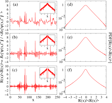
Figure 11: Numerical simulations of Eq. (1) in the focusing regime ($\sigma=+1$) for $t^{*}=20$. (a) Spatial fluctuations of $R(x)/<R(x)>=\Re{(\psi(x,t^{*}))}/<\Re{(\psi(x,t^{*}))}>$ that are found at the output of an ideal highpass frequency filter having a cutoff frequency $\xi=0$ (Eq. (6)) and (d) corresponding PDF of $R(x)/<R(x)>$. (b) and (e), same as (a) and (d) for $\xi=1$. (c) and (f), same as (a) and (d) for $\xi=2$. The insets in (a), (b), (c) represents the Fourier power spectra of the random fields plotted in (a), (b), (c).

Taking the wave system extensively described in Sec. II, we now consider the spatial fluctuations of the real part $\Re{(\psi(x,t^{*}))}$ of the complex field $\psi(x,t^{*})$ that has reached the stationary statistical state at $t^{*}=20$. In other words, the filtering process and the statistical treatment defined by Eqs. (6)-(8) are now applied to the random variable $R(x)=\Re{(\psi(x,t^{*}))}$. Spatial and statistical features found at the output of the highpass frequency filter are shown in Fig. 11 for the focusing regime.

When $\xi=0$, the random process $R(x)$ is not filtered and Fig. 11(a) shows the spatial evolution of the random variable $R(x)/<R(x)>=\Re{(\psi(x,t^{*}))}/<\Re{(\psi(x,t^{*}))}>$ in this situation. Fig. 11(d) represents the corresponding PDF of $R(x)/<R(x)>$. Without any filtering process, the heavy-tailed deviations from gaussianity shown in Fig. 11(d) are identical to those already shown in Fig. 4 but for $|\psi(x,t^{*})|^{2}$. Increasing the cutoff frequency $\xi$ of the ideal highpass filter (Eq.(6)), fluctuations of smaller and smaller scales are observed at the output of the highpass filter together with peaks of higher and higher amplitudes, see Fig. 11(b) and 11(c). Fig. 11(e) and Fig. 11(f) show that deviations from gaussianity become heavier when the cutoff frequency $\xi$ of the highpass filter is increased. These statistical features represent qualitative signatures of the intermittency phenomenon. Computing the kurtosis $\kappa(\xi)$ of $R(x)=\Re{(\psi(x,t^{*}))}$ for increasing values of the cutoff frequency $\xi$, we find a monotonic increase that complies with the definition of the intermittency phenomenon given by Frisch, see Fig. 13(a) Frisch:95 .

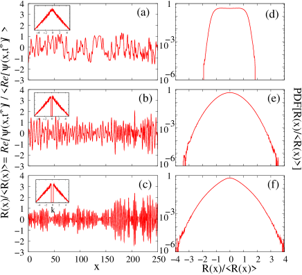
Figure 12: Numerical simulations of Eq. (1) in the defocusing regime ($\sigma=-1$) for $t^{*}=20$. (a) Spatial fluctuations of $R(x)/<R(x)>=\Re{(\psi(x,t^{*}))}/<\Re{(\psi(x,t^{*}))}>$ that are found at the output of an ideal highpass frequency filter having a cutoff frequency $\xi=0$ (Eq. (6)) and (d) corresponding PDF of $R(x)/<R(x)>$. (b) and (e), same as (a) and (d) for $\xi=1$. (c) and (f), same as (a) and (d) for $\xi=2$. The insets in (a), (b), (c) represents the Fourier power spectra of the random fields plotted in (a), (b), (c).

As shown in Fig. 12, features qualitatively similar to those described for the focusing regime are found in the defocusing regime. Fig. 12(a) (resp. Fig. 12 (d)) shows the spatial evolution (resp. the PDF) of $R(x)/<R(x)>=\Re{(\psi(x,t^{*}))}/<\Re{(\psi(x,t^{*}))}>$ for $\xi=0$, when the random process is not filtered. The low-tailed deviations from gaussianity shown in Fig. 12(d) are identical to those already shown in Fig. 7 but for $|\psi(x,t^{*})|^{2}$. They characterize the stationary statistical state found in the defocusing regime. Increasing the cutoff frequency $\xi$ of the ideal highpass filter (Eq.(6)), fluctuations of smaller and smaller scales are observed at the output of the highpass filter together with peaks of higher and higher amplitudes, see Fig. 12(b) and 12(c). Fig. 12(e) and Fig. 12(f) show that deviations from PDF computed for $\xi=0$ become heavier when the cutoff frequency $\xi$ of the highpass filter is increased. As shown in Fig. 13(b), the kurtosis $\kappa(\xi)$ monotonically increases with $\xi$, as for the focusing regime. Let us recall that a kurtosis $\kappa$ equal to $3$ corresponds to a random field having a gaussian statistics. The fact that the initial value of the kurtosis $\kappa(\xi=0)$ is lower (resp. greater) than $3$ in defocusing (resp. focusing) regime complies with the fact that the unfiltered field exhibit low-tailed (resp. heavy-tailed) deviations from gaussianity at $t^{*}=20$. Note that the growth of the kurtosis $\kappa(\xi)$ is greater in focusing regime than in defocusing regime, see Fig. 13.

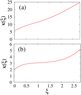
Figure 13: Numerical simulations of Eq. (1) for $t^{*}=20$. Evolution of the kurtosis $\kappa$ as a function of the cutoff frequency $\xi$ of the highpass filter defined by Eq. (6). (a) Focusing regime ($\sigma=+1$). (b) Defocusing regime ($\sigma=-1$).

V Conclusion

The work presented in this paper deals with the general question of statistical changes experienced by ensembles of nonlinear random waves propagating in systems ruled by integrable equations. It enters within the framework of “integrable turbulence” which is a new field of research introduced by Zakharov to address specifically this question that “composes a new chapter of the theory of turbulence” Zakharov:09 . In our work, we have specifically focused on optical fiber systems accurately described by the integrable one-dimensional nonlinear Schrödinger equation. We have considered random complex fields having a gaussian statistics and an infinite extension at initial stage. Numerical simulations with periodic boundary conditions and optical fiber experiments have been used to investigate spectral and statistical changes experienced by nonlinear waves both in focusing and in defocusing propagation regimes.

As a result of propagation in the strongly nonlinear regime, the power spectrum of the random waves is found to broaden while taking exponential wings both in focusing and in defocusing regimes, see Sec. II.2 and Sec. II.3. In the nonlinear regime, this spectral broadening phenomenon is a signature of a process in which the typical spatial scale of the random fluctuations decreases to reach the healing length of the wave system at long evolution time. Numerical simulations have revealed that heavy-tailed deviations from gaussian statistics occur in the focusing regime while low-tailed deviations from gaussian statistics are found in the defocusing regime. These statistical behaviors have been observed in optical fiber experiments relying on the implementation of an original and fast detection scheme, see Sec. III. Numerical simulations made at long evolution times have also shown that the wave system exhibits a statistically stationary state in which neither the PDF of the wave field nor the spectrum change with the evolution variable. Separating fluctuations of small scale from fluctuations of large scale, we have finally revealed the phenomenon of intermittency; i.e., small scales are characterized by large heavy-tailed deviations from Gaussian statistics, while the large ones are almost Gaussian. This intermittency phenomenon has been observed both in focusing and in defocusing propagation regimes, see Sec. IV.

As underlined in Sec. I, the determination of the PDF of a random wave field represents an issue of importance in the field of integrable turbulence. Given a nonlinear partial differential integrable equation together with some given initial and boundary conditions, there is no systematic theory that allows one to determine the PDF of the wave field at asymptotic stage (i.e. long evolution time).

The wave turbulence (WT) theory describes out-of-equilibrium statistical mechanics of random nonlinear waves in the weakly nonlinear regimeNazarenko ; Picozzi:07 . The WT theory is commonly used to treat wave systems that are ruled by non integrable equations and in which the long-time evolution is dominated by resonant interactions among waves (i.e. Fourier components). Using the closure of the statistical moments of the random field and neglecting non resonant interactions, kinetic equations describing the long-term evolution of the wave spectrum can be derived. However it has been shown that the short term evolution of WT can be influenced by non-resonant terms Annenkov:09 . In the specific case of the integrable 1D-NLSE, there are only trivial resonance conditions Suret:11 ; Picozzi:14 . As a result, collision terms found in the kinetic equations determined from the WT theory vanish Zakharov:09 ; Suret:11 ; Picozzi:14 . Using the closure of the moments and keeping the contribution of non resonant terms, it is however possible to derive “quasi-kinetic” equations that describe the evolution of the wave spectrum Janssen:03 ; Soh:10 ; Suret:11 . This approach has been used to study the evolution of the statistics both in focusing and defocusing case in ref. Janssen:03 . This kind of WT treatment has been shown to properly describe the evolution of the kurtosis of the wave field together with spectral changes that occur in the weakly nonlinear regime Janssen:03 ; Soh:10 ; Suret:11 .

There are now many open questions regarding integrable turbulence in the strongly nonlinear regime discussed throughout this paper. The inverse scattering theory (IST) provides a natural framework for the investigation of statistical properties of nonlinear wave systems ruled by integrable equations. In particular, IST has been used in ref. Derevyanko:12 to describe some experiments examining nonlinear diffraction of localized incoherent light beams Bromberg:10 . The theoretical description of this experiment can be made by using standard tools of the IST because it is fully compatible with the central assumption of IST that the wave field decays at infinity. IST has thus been used both in the focusing and in the defocusing regimes to determine some mathematical expressions for the PDF of the wave field Derevyanko:12 .

Our experiments and numerical simulations made with non-decaying and non-localized random waves open new questions about statistical properties of incoherent waves in integrable turbulence. First, the statistical properties characterizing the asymptotic stage of integrable turbulence are of fundamentally different natures for waves fluctuating around a constant background and for decaying waves. With continuous random waves having an infinite spatial extension, the nonlinear evolution of the random wave can no longer produce individualized solitons at long time. On the other hand, solitons never separate from each other and they always interact. Moreover solitons on finite background can emerge from nonlinear interaction in the focusing regime. In the defocusing case, the fact that the random field does not decay at infinity means that dark solitons can be sustained and interact at any time (any value of $z$ in our fiber experiments).

In our work, the relevant boundary conditions are periodic boundary conditions in a box of size $L$. Random waves of infinite spatial extension such as the ones considered in experiments reported in Sec. III can be described by taking the limit of a box of infinite spatial extension ($L\rightarrow\infty$). Rigorously speaking, the theoretical framework for dealing with integrable wave systems and periodic boundary conditions is finite gap theory osborne2010nonlinear . So far, no theoretical work has been made in this framework to determine statistical properties of ensembles of nonlinear random waves. However some recent results point out the possibility to use the inverse scattering transform for the focusing nonlinear Schrödinger equation with nonzero boundary conditions Biondini:14 .

The gaussian statistics of the initial condition is a key point of our experimental work. In the focusing regime of the 1D-NLSE, the statistics of the field measured in the statistically stationary state strongly depends on the nature of the initial condition. In our experiments and numerical simulations made with a complex field having initially a gaussian statistics, heavy-tailed deviations from gaussianity have been observed in the statistically stationary state (i.e. at long time), as discussed in Sec. II.2 and in Sec. III. If the initial condition is now made from a plane wave (or a condensate) with an additional noise, the nonlinear stage of modulational instability is characterized by a stationary statistics following the normal law Agafontsev:14c . The fact that there exists such a strong qualitative difference between statistics measured in the stationary state while starting from different noisy initial condition is an intriguing issue.

We hope that our results will stimulate new theoretical works aiming to understand the mechanisms leading to the strongly non gaussian statistics in focusing and defocusing 1D-NLSE systems with random initial conditions and non-zero boundary conditions.

Acknowledgments This work has been partially supported by Ministry of Higher Education and Research, Nord-Pas de Calais Regional Council and European Regional Development Fund (ERDF) through the Contrat de Projets Etat-Région (CPER) 2007–2013, as well as by the Agence Nationale de la Recherche through the LABEX CEMPI project (ANR-11-LABX-0007) and the OPTIROC project (ANR-12-BS04-0011 OPTIROC). S. R, P. W and P.S acknowledge Dr G. El for fruitful discussions. M.O. was supported by MIUR grant no. PRIN 2012BFNWZ2. M.O. thanks Dr B. Giulinico for fruitful discussions.

References

- (1) S. K. Turitsyn S. A. Babin, A. E. El-Taher, P. Harper, D. V. Churkin, S. I. Kablukov, J. D. Ania-Castanon, V. Karalekas, E. V. Podivilov, Nature Photonics, 4, 231 (2015).
- (2) P.Walczak, S. Randoux and P. Suret, Opt. Lett. 40, 3101 (2015).
- (3) S. Randoux, P. Walczak, M. Onorato, P. Suret, Phys. Rev. Lett. 113, 113902 (2014).
- (4) Zhang H. D., Guedes Soares C., Cherneva, Z., Onorato, M., Natural Hazards and Earth System Science, 14, 959 (2014).
- (5) Dudley John M., Dias Frederic, Erkintalo Miro and Genty, Goery, Nat. Photon., 8, 755 (2014).
- (6) Agafontsev D. S. and Zakharov V.E., ArXiv, 1409.4692, (2014).
- (7) Agafontsev D.S. and Zakharov V. E., ArXiv, 1404.6088, ( 2014)
- (8) Kibler B., Fatome J., Finot C., Millot G., Genty G., Wetzel B., Akhmediev N.,Dias F. and Dudley J. M, Scientific Reports, 2, (2012)
- (9) Mussot A., Beaugeois M., Bouazaoui M. and Sylvestre T., Opt. Express 15, 11553 (2007).
- (10) J. M. Dudley, G. Genty, F. Dias, B. Kibler and N. Akhmediev, Opt. Express 17, 21497 (2009).
- (11) Optics Commun., 13, 96 (1975)
- (12) Duguay M. A. and Hansen J. W., Applied Physics Letters, 13, 178 (1968).
- (13) A. Picozzi, Opt. Express, 15, 9063 (2007).
- (14) P. Suret, A. Picozzi and S. Randoux, Opt. Express 18, 17852 (2011).
- (15) S. Randoux, G. Beck, F. Anquez, G. Melin, L. Bigot, M. Douay and Pierre Suret, Journal of Lightwave Technology, 27, 1580 (2009).
- (16) E.N. Pelinovsky, E.G. Shurgalina, A.V. Sergeeva, T.G. Talipova, G.A. El and R.H.J. Grimshaw, Physics Letters A , 377, 272 (2013).
- (17) Derevyanko S. and Small E., Physical Review A, 85 053816 (2012).
- (18) Nonlinear random waves, Konotop V. and Vázquez L., World Scientific (1994).
- (19) Extreme ocean waves, Pelinovsky E. and Kharif C., Springer (2008).
- (20) S. A. Babin, D. V. Churkin, A. E. Ismagulov, S. I. Kablukov and E. V. Podivilov, J. Opt. Soc. Am. B, 24, 1729 (2007).
- (21) E. G. Turitsyna, S. V. Smirnov, S. Sugavanam, N. Tarasov, X. Shu, S.A. Babin, E.V. Podivilov, D.V. Churkin, G. Falkovich and S.K. Turitsyn, Nat. Photon., 7, 783 (2013).
- (22) Y. Bromberg, U. Lahini, E. Small and Y. Silberberg, Nat. Photon., 4, 721 (2010).
- (23) D. R. Solli, C. Ropers, P. Koonath and B. Jalali, Nature, 450, 1054 (2007).
- (24) Y. Q. Xu and S. G. Murdoch, Opt. Lett., 6, 826 (2010).
- (25) Bonatto C., Feyereisen M.,Barland S., Giudici M., Masoller C., Leite J. and Tredicce, J. R., Phys. Rev. Lett., 107, 053901 (2011).
- (26) Kibler B., Finot C. and Dudley J. M., European Physical Journal Special Topics, 173, 289 (2009).
- (27) Jalali B., Solli D. R., Goda K, Tsia K and Ropers C, European Physical Journal Special Topics, 185, 145 (2010).
- (28) Montina A., Bortolozzo U., Residori S. and Arecchi F. T., Phys. Rev. Lett., 103, 173901 (2009).
- (29) Lafargue C., Bolger J., Genty G., Dias F., Dudley J.M. and Eggleton B.J., Electronics Letters, 45, 217 (2009).
- (30) M. Erkintalo, G. Genty and J. M. Dudley, Opt. Lett., 16, 2468 (2009).
- (31) J.M. Dudley, C. Finot, G. Millot, J. Garnier, G. Genty, D. Agafontsev and F. Dias, The European Physical Journal Special Topics, 185, 125 (2010).
- (32) Nonlinear Fiber optics, G. P. Agrawal, Academic Press (2001).
- (33) Erkintalo M., Genty G. and Dudley J.M., The European Physical Journal Special Topics, 185, 135 (2010).
- (34) K. Hammani, B. Kibler, C. Finot and A. Picozzi”, Phys. Lett. A , 374, 3585 (2010).
- (35) J. Kasparian, P. Béjot, J. P. Wolf and John M. Dudley, Opt. Express, 14, 12070 (2009).
- (36) K. Hammani, C. Finot, J. M. Dudley and Guy Millot, Opt. Express, 21, 16467 (2008).
- (37) H. Rhee and T. Joo, Opt. Lett., 30, 96 (2005).
- (38) M. Nobuhito, M. Onorato and P. A. E. M. Janssen, J. Phys. Oceanogr., 41, 1484 (2011).
- (39) Janssen P. A. E. M. and Onorato M., J. Phys. Oceanogr., 37, (2007).
- (40) Zakharov V. E., Studies in Applied Mathematics, 122, 219, (2009).
- (41) Zakharov V. E. and Gelash A. A., Phys. Rev. Lett., 111, 054101 (2013).
- (42) P. A. E. M. Janssen, J. Phys. Oceanogr., 33, 863 (2003).
- (43) Agafontsev, D.S., JETP Letters 98, 731 (2014).
- (44) Pisarchik A. N., J. Rider, Sevilla-Escoboza R., Huerta-Cuellar G. and Taki M., Phys. Rev. Lett., 107, 274101 (2011).
- (45) Statistical optics, Goodman, J. W. , New York, Wiley-Interscience (1985).
- (46) Optical Coherence and Quantum Optics, Mandel L. and Wolf E., Cambridge University Press (1995).
- (47) Fundamentals of Photonics: Second Edition, Saleh, B. E. A. and Teich, M. C. , John Wiley & Son (2007).
- (48) Kolmogorov Spectra of Turbulence I, V.E. Zakharov, V.S. L’vov and G. Falkovich, Springer, Berlin (1992).
- (49) A. Picozzi, J. Garnier, T. Hansson, P. Suret, S. Randoux, G. Millot and D.N. Christodoulides, Physics Reports , 542, 1 (2014).
- (50) Wave Turbulence, Sergey Nazarenko, Lecture Notes in Physics, Springer, Berlin (2011).
- (51) S. Dyachenko, A.C. Newell, A. Pushkarev and V.E. Zakharov, Physica D, 57, 96 (1992).
- (52) M. Onorato, S. Residori, U. Bortolozzo, A. Montina and F.T. Arecchi, Physics Reports , 528, 47 (2013).
- (53) N. Akhmediev, J.M. Soto-Crespo and A. Ankiewicz, Phys. Lett. A , 373, 2137 (2009).
- (54) Ankiewicz A., Soto-Crespo J. M. and Akhmediev N., Phys. Rev. E, 81, 046602 (2010).
- (55) Kudlinski A., Barviau B., Leray A., Spriet C., Heliot L. and Mussot A., Opt. express, 18, 27445 (2010).
- (56) B. Barviau, S. Randoux and P. Suret, Opt. Lett., 31, 1696 (2006).
- (57) N. Akhmediev A. Ankiewicz and M. Taki, Physics Letters A , 373, 675 (2009).
- (58) A. Mussot, A. Kudlinski, M. Kolobov, E. Louvergneaux, M. Douay and M. Taki, Opt. Express, 19, 17010 (2009).
- (59) S. Randoux, N. Dalloz and P. Suret, Opt. Lett., 6, 790 (2011).
- (60) S. Randoux and P. Suret, Opt. Lett., 37, 500 (2012).
- (61) Solli D. R., Herink G., Jalali B. and Ropers C., Nature Photonics, 6, 463 (2012).
- (62) N. Akhmediev, J. M. Dudley, D. R. Solli and S. K. Turitsyn, Journal of Optics, 15, 060201 (2013).
- (63) Goda K. and Jalali B., Nature Photonics, 7, 102 (2013).
- (64) Wetzel B., Stefani A., Larger L., Lacourt P., Merolla J., Sylvestre T., Kudlinski A., Mussot A., Genty G., Dias F. and J.M. Dudley, Scientific reports, 2, (2012).
- (65) Iafrati A., Babanin A. and Onorato M., Phys. Rev. Lett., 110, 184504 (2013).
- (66) Marsch E. and Tu C-Y, Nonlinear processes in Geophysics, 4, 101 (1999).
- (67) Lecaplain C., Grelu P., Soto-Crespo J. M. and Akhmediev N., Phys. Rev. Lett. 108, 233901 (2012).
- (68) Onorato M., Osborne A. R., Serio M. and Cavaleri L., Physics of Fluids 17, 078101 (2005).
- (69) Onorato M., Osborne A. R., Serio M., Cavaleri L., Brandini C., Stansberg C. T., Phys. Rev. E 70, 067302 (2004).
- (70) Onorato M., Osborne A. R., Serio M. and Bertone S., Phys. Rev. Lett. 86, 5831 (2001).
- (71) Chabchoub A., Hoffmann N., Onorato M., Genty G., Dudley J. M., Akhmediev N., Phys. Rev. Lett. 111, 054104 (2013).
- (72) Chabchoub A., Hoffmann N. P. and Akhmediev N., Phys. Rev. Lett. 106, 204502 (2011).
- (73) Kibler B., Hammani K., Michel C., Finot C. and Picozzi A., Physics Letters A 375, 3149 (2011).
- (74) Frisquet B., Kibler B. and Millot G., Physical Review X 3, 041032 (2013).
- (75) Solli D. R., Ropers C. and Jalali B., Physical review letters 101, 233902 (2008)
- (76) Kibler B., Fatome J., Finot C., Millot G., Dias F., Genty G., Akhmediev N. and Dudley J. M., Nature Physics, 6, 790 (2010).
- (77) Fatome J., Finot C., Millot G., Armaroli A. and Trillo S., Phys. Rev. X 4, 021022 (2014).
- (78) Nonlinear Optics, R. W. Boyd, Academic Press (1992).
- (79) Islas A. L. and Schober C. M., Physics of Fluids 17 (2005)
- (80) Walczak P., Randoux S. and Suret P., Phys. Rev. Lett. 114, 143903, (2015).
- (81) Optical Coherence and Quantum Optics, L. Mandel and E. Wolf, Cambridge University Press (1995).
- (82) Toenger S., Godin T., Billet C., Dias F., Erkintalo M., Genty G. and Dudley J. M., Sci. Rep. 5 (2015).
- (83) Turbulence, the legacy of A.N. Kolmogorov, U. Frisch, Cambridge University Press (1995).
- (84) Nazarenko S., Lukaschuk S., McLelland S. and Denissenko P., Journal of Fluid Mechanics 642, 395 (2010).
- (85) Falcon E., Fauve S. and Laroche C., Phys. Rev. Lett. 98, 154501 (2007).
- (86) E. Falcon, S. G. Roux and C. Laroche, Europhysics Lett. 90, 34005 (2010).
- (87) Bosch E. and van de Water W., Phys. Rev. Lett. 70, 3420 (1993).
- (88) Sreenivasan K. R., Journal of Fluid Mechanics 151, 81 (1985).
- (89) O. Alexandrova, V. Carbone, P. Veltri and L. Sorriso-Valvo, Planetary and Space Science 55, 2224 (2007).
- (90) M. Conforti and S. Trillo, Opt. Lett. 38, 3815 (2013).
- (91) Moro A. and Trillo S., Phys. Rev. E 89, 023202 (2014).
- (92) Conforti M., Baronio F. and Trillo S., Phys. Rev. A, 89, 013807 (2014).
- (93) El G. A., Grimshaw R. H. J. and Kamchatnov A. M., Studies in Applied Mathematics 114, 395 (2005).
- (94) Efimov A., Yulin A. V., Skryabin D. V., Knight J. C., Joly, N., Omenetto, F. G.,Taylor A. J. and Russell P., Phys. Rev. Lett. 95, 213902 (2005).
- (95) Böhm M. and Mitschke F., Phys. Rev. E, 73, 066615 (2006).
- (96) Derevyanko S. A. and Prilepsky J. E., Phys. Rev. E 78, 046610 (2008).
- (97) F. G. Bass, Y. S. Kivshar and V. V. Konotop, Sov. Phys. JETP 65, 245 (1987).
- (98) Fratalocchi A., Conti, C., Ruocco G. and Trillo S., Phys. Rev. Lett. 101, 044101 (2008).
- (99) El G. A. and Kamchatnov A. M., Phys. Rev. Lett. 95, 204101 (2005).
- (100) Fermi E., Pasta J. and Ulam S, Studies of nonlinear problems, Los Alamos Scientific Laboratory Report No. LA-1940 (1955).
- (101) Zabusky N. J. and Kruskal M. D., Phys. Rev. Lett. 15, 240 (1965).
- (102) Zakharov V. E. and Shabat P. B., Sov. Phys. JETP 34, 62 (1972).
- (103) Ma Y.C., Studies in Applied Mathematics 60, 43 (1979).
- (104) Kuznetsov E. A., Akademiia Nauk SSSR Doklady 236, 575 (1977).
- (105) Peregrine D. H., J. Austral. Math. Soc. Ser. B 25, 16 (1983).
- (106) Akhmediev N. N., Eleonskii V. M. and Kulagin N.E., Sov. Phys. JETP, 62, 894 (1985).
- (107) Dysthe K. B. and Trulsen K., Physica Scripta, T82, 48 (1999).
- (108) Osborne A. R., Onorato, M. and Serio M., Phys. Lett. A 275, 386 (2000).
- (109) Onorato M., Residori S., Bortolozzo U., Montina A. and Arecchi F. T., Physics Reports 528, 47 (2013).
- (110) Nonlinear ocean waves, Osborne A., Academic Press (2010).
- (111) Rogue waves in the ocean, Kharif C., Pelinovsky E. and Slunyaev A., Springer Verlag (2009).
- (112) Chabchoub A., Hoffmann N., Onorato M., Akhmediev N., Physical Review X 2, 011015 (2012).
- (113) Miles J. W., J. Fluid Mech. 3, 185 (1957).
- (114) Janssen P. A. E. M., J. Phys. Oceanogr. 21, 1631 (1991).
- (115) Onorato M., Osborne A. R., Serio M. and Damiani T., Rogue Wave 2000, 181 (2000).
- (116) Chabchoub A., Kibler B., Finot C., Millot G., Onorato M., Dudley J. M. and Babanin A. V., Annals of Physics 361, 490 (2015).
- (117) Conforti M., Mussot A., Fatome J., Picozzi A., Pitois S., Finot C., Haelterman M., Kibler B., Michel C. and Millot G., Phys. Rev. A, 91, 023823 (2015).
- (118) Taki M., Mussot A., Kudlinski A., Louvergneaux E., Kolobov M., Douay M., Physics Letters A 374, 691 (2010).
- (119) Michel C., Haelterman M., Suret P., Randoux S., Kaiser R. and Picozzi A., Physical Review A 84, 033848 (2011).
- (120) Churkin D. V., Smirnov S. V. and Podivilov E. V., Optics letters 35, 3288 (2010).
- (121) O. A. Gorbunov, S. Sugavanam and D.V. Churkin, Opt. Express 22, 28071 (2014).
- (122) Biondini G. and Kovačič G., Journal of Mathematical Physics 55, 031506 (2014)
- (123) D. B. S. Soh, J. P. Koplow,S. W. Moore, K. L. Schroder and W. L. Hsu, Opt. Express 18, 22393 (2010).
- (124) Annenkov S. Y. and Shrira V. I., Phys. Rev. Lett. 102, 024502 (2009).