Planck 2015 results. XXIII. The thermal
Sunyaev-Zeldovich effect–cosmic infrared background correlation

We use Planck data to detect the cross-correlation between the thermal Sunyaev-Zeldovich (tSZ) effect and the infrared emission from the galaxies that make up the the cosmic infrared background (CIB). We first perform a stacking analysis towards Planck-confirmed galaxy clusters. We detect infrared emission produced by dusty galaxies inside these clusters and demonstrate that the infrared emission is about 50 % more extended than the tSZ effect. Modelling the emission with a Navarro–Frenk–White profile, we find that the radial profile concentration parameter is $c_{500}=1.00^{+0.18}_{-0.15}$. This indicates that infrared galaxies in the outskirts of clusters have higher infrared flux than cluster-core galaxies. We also study the cross-correlation between tSZ and CIB anisotropies, following three alternative approaches based on power spectrum analyses: (i) using a catalogue of confirmed clusters detected in Planck data; (ii) using an all-sky tSZ map built from Planck frequency maps; and (iii) using cross-spectra between Planck frequency maps. With the three different methods, we detect the tSZ-CIB cross-power spectrum at significance levels of (i) 6 $\sigma$, (ii) 3 $\sigma$, and (iii) 4 $\sigma$. We model the tSZ-CIB cross-correlation signature and compare predictions with the measurements. The amplitude of the cross-correlation relative to the fiducial model is $A_{\rm tSZ-CIB}=1.2\pm 0.3$. This result is consistent with predictions for the tSZ-CIB cross-correlation assuming the best-fit cosmological model from Planck 2015 results along with the tSZ and CIB scaling relations.

1 Introduction

This paper is one of a set associated with the 2015 release of data from the Planck mission. It reports the first all-sky detection of the cross-correlation between the thermal Sunyaev-Zeldovich (tSZ) effect (Sunyaev & Zeldovich 1969, 1972) and the cosmic infrared background (CIB; Puget et al. 1996; Fixsen et al. 1998; Hauser et al. 1998). An increasing number of observational studies are measuring the tSZ effect and CIB fluctuations at infrared and submillimetre wavelengths, including investigations of the CIB with the Spitzer Space Telescope (Lagache et al. 2007) and the Herschel Space Observatory (Amblard et al. 2011; Viero et al. 2012, 2015), and observations of the tSZ effect with instruments such as the Atacama Pathfinder Experiment (Halverson et al. 2009) and Bolocam (Sayers et al. 2011). In addition, a new generation of CMB experiments can measure the tSZ effect and CIB at microwave frequencies (Hincks et al. 2010; Hall et al. 2010; Dunkley et al. 2011; Zwart et al. 2011; Reichardt et al. 2012; Planck Collaboration XXI 2014; Planck Collaboration XXX 2014).

The large frequency coverage of Planck, from 30 to 857 GHz, makes it sensitive to both of these important probes of large-scale structure. At intermediate frequencies, from 70 to 217 GHz, the sky emission is dominated by the cosmic microwave background (CMB). At these frequencies, it is possible to detect galaxy clusters that produce a distortion of the CMB blackbody emission through the tSZ effect. At the angular resolution of Planck, this effect is mainly produced by local ($z<1$) and massive galaxy clusters in dark matter halos (above $10^{14}\thinspace{\rm M_{\odot}}$), and it has been used for several studies of cluster physics and cosmology (e.g., Planck Collaboration X 2011; Planck Collaboration XI 2011; Planck Collaboration Int. III 2013; Planck Collaboration Int. V 2013; Planck Collaboration Int. VIII 2013; Planck Collaboration Int. X 2013; Planck Collaboration XX 2014; Planck Collaboration XXIV 2015; Planck Collaboration XX 2014; Planck Collaboration XXIV 2015). At frequencies above 353 GHz, the sky emission is dominated by thermal emission, both Galactic and extragalactic (Planck Collaboration XI 2014; Planck Collaboration XXX 2014). The dominant extragalactic signal is the thermal infrared emission from dust heated by UV radiation from young stars. According to our current knowledge of star-formation history, the CIB emission has a peak in its redshift distribution between $z=1$ and $z=2$, and is produced by galaxies in dark matter halos of $10^{11}$–$10^{13}\thinspace{\rm M_{\odot}}$; this has been confirmed through the measured strong correlation between the CIB and CMB lensing (Planck Collaboration XVIII 2014). However, due to the different redshift and mass ranges, the CIB and tSZ distributions have little overlap at the angular scales probed by Planck, making this correlation hard to detect.

Nevertheless, determining the strength of this tSZ-CIB correlation is important for several reasons. Certainly we need to know the extent to which tSZ estimates might be contaminated by CIB fluctuations, but uncertainty in the correlation also degrades our ability to estimate power coming from the “kinetic” SZ effect (arising from peculiar motions), which promises to probe the reionization epoch (e.g., Mesinger et al. 2012; Reichardt et al. 2012; Planck Collaboration Int. XXXVII 2015). But as well as this, analysis of the tSZ-CIB correlation allows us to better understand the spatial distribution and evolution of star formation within massive halos.

The profile of infrared emission from galaxy clusters is expected to be less concentrated than the profile of the number counts of galaxies. Indeed, core galaxies present reduced infrared emission owing to quenching, which occurs after they make their first passage inside $r\simeq R_{500}$ (Muzzin et al. 2014). Using SDSS data, Weinmann et al. (2010) computed the radial profile of passive galaxies for high-mass galaxy clusters ($M>10^{14}\thinspace{\rm M_{\odot}}$). They found that the fraction of passive galaxies is 70–80 % at the centres and 25–35 % in the outskirts of clusters. The detection of infrared emission cluster by cluster is difficult at millimetre wavelengths, since the emission is faint and confused by the fluctuations of the infrared sky (Galactic thermal dust and CIB). Statistical detections of infrared emission in galaxy clusters have been made by stacking large samples of known clusters (Montier & Giard 2005; Giard et al. 2008; Roncarelli et al. 2010) in IRAS data (Wheelock et al. 1993). The stacking approach has also been shown to be a powerful method for extracting the tSZ signal from microwave data (e.g., Lieu et al. 2006; Diego & Partridge 2009).

Recently, efforts have been made to model the tSZ-CIB correlation (e.g., Zahn et al. 2012; Addison et al. 2012). Using a halo model, it is possible to predict the tSZ-CIB cross-correlation. The halo model approach allows us to consider distinct astrophysical emission processes that trace the large-scale dark matter density fluctuation, but have different dependencies on the host halo mass and redshift. In this paper, we use models of the tSZ-CIB cross-correlation at galaxy cluster scales. We note that the tSZ effect does not possess significant substructure on the scale of galaxies, so the tSZ-CIB cross-correlation should not possess a shot noise term.

Current experiments have already provided constraints on the tSZ-CIB cross-correlation at low frequencies, between 100 and 250 GHz. The ACT collaboration set an upper limit $\rho<0.2$ on the tSZ-CIB cross correlation (Dunkley et al. 2013). George et al. (2014), using SPT data and assuming a single correlation factor, obtained a tSZ-CIB correlation factor of $0.11^{+0.06}_{-0.05}$; a zero correlation is disfavoured at a confidence level of 99 %.

Our objective in this paper is twofold. First, we characterize the CIB emission toward tSZ-detected galaxy clusters by constraining the profile and redshift dependence of CIB emission from galaxy clusters. Then, we set constraints on the overall tSZ-CIB cross-correlation power spectrum, and report the first all-sky detection of the tSZ-CIB angular cross-power spectra, at a significance level of $4\thinspace\sigma$. Our models and results on the tSZ-CIB cross-correlation have been used in a companion Planck paper Planck Collaboration XXII (2015).

In the first part of Sect. 2, we explain our modelling approach for the tSZ effect and CIB emission at the galaxy cluster scale. In the second part of Sect. 2, we describe the model for the tSZ, CIB, and tSZ-CIB power and cross-power spectra using a halo model. Then in Sect. 3 we present the data sets we have used. Sections 4 and 5 present our results for the SED, shape, and cross-spectrum of the tSZ-CIB correlation. Finally, in Sect. 6 we discuss the results and their consistency with previous analyses.

Throughout this paper, the tSZ effect intensity will be expressed in units of Compton parameter, and we will use the best-fit cosmology from Planck Collaboration XIII (2015, fourth column of table 3) using “TT,TE,EE+lowP” values as the fiducial cosmological model, unless otherwise specified. Thus, we adopt $H_{0}=67.27\thinspace{\rm km}\thinspace{\rm s}^{-1}\thinspace{\rm Mpc}^{\-1}$, $\sigma_{8}=0.831$, and $\Omega_{\rm m}=0.3156$.

2 Modelling

To model the cross-correlation between tSZ and CIB anisotropies we have to relate the mass, $M_{500}$, and the redshift, $z$, of a given cluster to tSZ flux, $Y_{500}$, and CIB luminosity $L_{500}$. We define $M_{500}$ (and $R_{500}$) as the total mass (and radius) for which the mean over-density is 500 times the critical density of the Universe. Considering that the tSZ signal in the Planck data has no significant substructure at galaxy scales, we modelled the tSZ-CIB cross-correlation at the galaxy cluster scale. This can be considered as a large-scale approximation for the CIB emission, and at the Planck angular resolution it agrees with the more refined modelling presented in Planck Collaboration XXX (2014).

Table 1: Cosmological and scaling-law parameters for our fiducial model, for both the $Y_{500}$–$M_{500}$ relation (Planck Collaboration XX 2014) and the $L_{500}$–$M_{500}$ relation (fitted to spectra from Planck Collaboration XXX 2014).

Planck-SZ cosmology $$\Omega_{\rm m} \kern 4.00002pt0.29\pm 0.02 \sigma_{8} \kern 4.00002pt0.77\pm 0.02 H_{0} 67.3\pm 1.4 \Omega_{\rm m} \kern 4.00002pt0.316\pm 0.009 \sigma_{8} \kern 4.00002pt0.831\pm 0.013 H_{0} 67.27\pm 0.66 M_{500} Y_{500} {\rm log}\thinspace Y_{\ast} -0.19\pm 0.02 \alpha_{\rm SZ} \kern 6.22224pt1.79\pm 0.08 \beta_{\rm SZ} \kern 6.22224pt0.66\pm 0.50 M_{500} L_{500} T_{0} 24.4\pm 1.9 \alpha_{\rm CIB} \kern 4.00002pt0.36\pm 0.05 \beta_{\rm CIB} \kern 4.00002pt1.75\pm 0.06 \gamma_{\rm CIB} \kern 4.00002pt1.70\pm 0.02 \delta_{\rm CIB} \kern 4.00002pt3.2\kern 4.00002pt\pm 0.2\kern 4.00002pt \epsilon_{\rm CIB} \kern 4.00002pt1.0\kern 4.00002pt\pm 0.1\kern 4.00002pt$$. . . Planck-CMB cosmology . . . – . . . – . . . . . .

2.1 The thermal Sunyaev-Zeldovich effect

The tSZ effect is a small-amplitude distortion of the CMB blackbody spectrum caused by inverse-Compton scattering (see, e.g., Rephaeli 1995; Birkinshaw 1999; Carlstrom et al. 2002). Its intensity is related to the integral of the pressure along the line of sight via the Compton parameter, which for a given direction on the sky is

$$y=\int\frac{k_{\rm B}\sigma_{\rm T}}{m_{\rm e}c^{2}}n_{\rm e}T_{\rm e}{\rm d}l.$$ (1)

Here ${\rm d}l$ is the distance along the line of sight, $k_{\rm B}$, $\sigma_{\rm T}$, $m_{\rm e}$, and $c$ are the usual physical constants, and $n_{\rm e}$ and $T_{\rm e}$ are the electron number density and the temperature, respectively.

In units of CMB temperature, the contribution of the tSZ effect to the submillimetre sky intensity for a given observation frequency $\nu$ is given by

$$\frac{\Delta T_{\rm CMB}}{T_{\rm CMB}}=g(\nu)y.$$ (2)

Neglecting relativistic corrections we have $g(\nu)=x\coth(x/2)-4$, with $x=h\nu/(k_{\rm B}T_{\rm CMB})$. The function $g(\nu)$ is is equal to 0 at about 217 GHz, and is negative at lower frequencies and positive at higher frequencies.

We have used the $M_{500}$–$Y_{500}$ scaling law presented in Planck Collaboration XX (2014),

$$E^{-\beta_{\rm SZ}}(z)\left[\frac{D^{2}_{\rm A}(z){Y}_{500}}{10^{-4}\thinspace{\rm Mpc}^{2}}\right]=Y_{\ast}\left[\frac{h}{0.7}\right]^{-2+\alpha_{\rm SZ}}\left[\frac{(1-b)M_{500}}{6\times 10^{14}\thinspace{\rm M_{\odot}}}\right]^{\alpha_{\rm SZ}},$$ (3)

with $E(z)=\sqrt{\Omega_{\rm m}(1+z)^{3}+\Omega_{\Lambda}}$ for a flat universe. The coefficients $Y_{\ast}$, $\alpha_{\rm SZ}$, and $\beta_{\rm SZ}$ are taken from Planck Collaboration XX (2014), and are given in Table 1. The mean bias, $(1-b)$, between X-ray mass and the true mass is discussed in detail in Planck Collaboration XX (2014, appendix A) and references therein. We adopt $b=0.3$ here, which, given the chosen cosmological parameters, allows us to reproduce the tSZ results from Planck Collaboration XXII (2015) and Planck Collaboration XXIV (2015).

2.2 Cosmic infrared background emission

The CIB is the diffuse emission from galaxies integrated throughout cosmic history (see, e.g., Hauser & Dwek 2001; Lagache et al. 2005), and is thus strongly related to the star-formation rate history. The CIB intensity, $I(\nu)$, at frequency $\nu$ can be written as

$$I(\nu)=\int{\rm d}z\frac{{\rm d}\chi(z)}{{\rm d}z}\thinspace\frac{j(\nu,z)}{(1+z)},$$ (4)

with $\chi(z)$ the comoving distance and $j(\nu,z)$ the emissivity that is related to the star-formation density, $\rho_{\rm SFR}$, through

$$j(\nu,z)=\frac{\rho_{\rm SFR}(z)(1+z)\Theta_{\rm eff}(\nu,z)\chi^{2}(z)}{K},$$ (5)

where $K$ is the Kennicutt (1998) constant (SFR/$L_{\rm IR}=1.7\times 10^{-10}\thinspace{\rm M_{\odot}}\thinspace{\rm yr}^{-1}$) and $\Theta_{\rm eff}(\nu,z)$ the mean spectral energy distribution (SED) of infrared galaxies at redshift $z$.

To model the $L_{500}$–$M_{500}$ relation we use a parametric relation proposed by Shang et al. (2012) that relates the CIB flux, $L_{500}$, to the mass, $M_{500}$, as follows:

$$L_{500}(\nu)=L_{0}\left[\frac{M_{500}}{1\times 10^{14}\thinspace{\rm M_{\odot}}}\right]^{\epsilon_{\rm CIB}}\Psi(z)\thinspace\Theta\left[(1+z)\nu,T_{\rm d}(z)\right],$$ (6)

where $L_{0}$ is a normalization parameter, $T_{\rm d}(z)=T_{{\rm d}0}(1+z)^{\alpha_{\rm CIB}}$ and $\Theta\left[\nu,T_{\rm d}\right]$ is the typical SED of a galaxy that contributes to the total CIB emission,

$$\Theta\left[\nu,T_{\rm d}\right]=\left\{\begin{array}[]{ll}\nu^{\thinspace\beta_{\rm CIB}}B_{\nu}(T_{\rm d}),&\mbox{if}\ \nu<\nu_{0},\\ \nu^{-\gamma_{\rm CIB}},&\mbox{if}\ \nu\geq\nu_{0},\end{array}\right.$$

with $\nu_{0}$ being the solution of ${\rm d\thinspace log}[\nu^{\thinspace\beta_{\rm CIB}}B_{\nu}(T_{\rm d})]/{\rm d\thinspace log}(\nu)=-\gamma_{\rm CIB}$. We assume a redshift dependence of the form

$$\Psi(z)=(1+z)^{\delta_{\rm CIB}}.$$ (7)

We also define $S_{500}$ as

$${S}_{500}(\nu)=\frac{L_{500}(\nu)}{4\pi(1+z)\chi^{2}(z)}.$$ (8)

The coefficients $T_{{\rm d}0}$, $\alpha_{\rm CIB}$, $\beta_{\rm CIB}$, $\gamma_{\rm CIB}$, and $\delta_{\rm CIB}$ from Planck Collaboration XXX (2014) are given in Table 1. We fix the value of $\epsilon_{\rm CIB}$ to 1. In Sect. 2.5, this model of the CIB emission will be compared with the Planck measurement of the CIB power spectra. We stress that this parametrization can only be considered accurate at scales where galaxy clusters are not (or only marginally) extended. This is typically the case at Planck angular resolution for the low-mass and high-redshift dark matter halos that dominate the total CIB emission.

2.3 Angular power spectra

2.3.1 The halo model

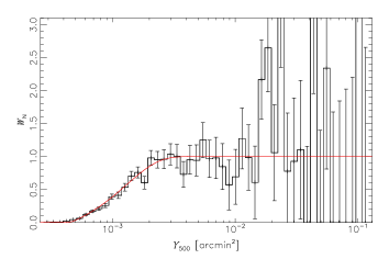
Figure 1: Weight of the mass function as a function of $Y_{500}$. Black: the ratio between the number of observed clusters and the predicted number of clusters from the Planck-SZ best-fit cosmology. Red: parametric formula, Eq. (12), for the selection function.

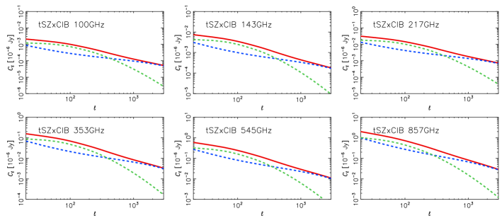
Figure 2: Predicted tSZ-CIB cross-correlation from 100 to 857 GHz for the fiducial model, where the tSZ signal is expressed in Compton parameter units. The blue dashed line presents the prediction for the 1-halo term, the green dashed line for the 2-halo term and the red solid line for the total model.

To model tSZ, CIB, and tSZ-CIB angular power spectra, we consider the halo-model formalism (see, e.g. Cooray & Sheth 2002) and the following general expression

$$C_{\ell}=C^{AB,{\rm 1h}}_{\ell}+C^{AB,{\rm 2h}}_{\ell},$$ (9)

where $A$ and $B$ stand for tSZ effect or CIB emission, $C^{AB,{\rm 1h}}_{\ell}$ is the 1-halo contribution, and $C^{AB,{\rm 2h}}_{\ell}$ is the 2-halo term that accounts for correlation in the spatial distribution of halos over the sky.

The 1-halo term $C^{AB,{\rm 1h}}_{\ell}$ is computed using the Fourier transform of the projected profiles of signals $A$ and $B$ weighted by the mass function and the $A$ and $B$ emission (see, e.g., Komatsu & Seljak 2002, for a derivation of the tSZ angular power spectrum):

$$C_{\ell}^{AB,{\rm 1h}}=4\pi\int{\rm d}z\frac{{\rm d}V}{{\rm d}z{\rm d}\Omega}\int{\rm d}M\frac{{\rm d^{2}N}}{{\rm d}M{\rm d}V}W^{A,{\rm 1h}}W^{B,{\rm 1h}},$$ (10)

where ${\rm d}^{2}N/{\rm d}M{\rm d}V$ is the dark-matter halo mass function from Tinker et al. (2008), ${\rm d}V/{\rm d}z{\rm d}\Omega$ is the comoving volume element, and $W^{A,{\rm 1h}}$, $W^{B,{\rm 1h}}$ are the window functions that account for selection effects and total halo signal. For the tSZ effect, we have $W^{\rm 1h}_{\rm tSZ}=W_{\rm N}(Y_{500}){Y}_{500}y_{\ell}(M_{500},z)$ and $W_{\rm N}(Y_{500})$ is a weight, ranging from 0 to 1, applied to the mass function to account for the effective number of clusters used in our analysis; here ${Y}_{500}$ is the tSZ flux, and $y_{\ell}$ is the Fourier transform of the tSZ profile. For the CIB emission we have $W^{\rm 1h}_{\rm CIB}={S}_{500}(\nu)I_{\ell}(M_{500},z)$, where $I_{\ell}$ the Fourier transform of the infrared profile (from Eq. 18) and ${S}_{500}(\nu)$ is given in Eq. (8).

The results for the radial analysis in Sect. 4.1.3 show that the infrared emission profile can be well approximated by an NFW profile (Navarro et al. 1997) with a concentration parameter $c_{500}=1.0$. The galaxy cluster pressure profile is modelled by a generalized NFW profile (GNFW, Nagai et al. 2007) using the best-fit values from Arnaud et al. (2010).

The contribution of the 2-halo term, $C^{AB,{\rm 2h}}_{\ell}$, accounts for large-scale fluctuations in the matter power spectrum that induce correlations in the dark-matter halo distribution over the sky. It can be computed as

$$C_{\ell}^{AB,{\rm 2h}}=4\pi \int{\rm d}z\frac{{\rm d}V}{{\rm d}z{\rm d}\Omega}\left(\int{\rm d}M\frac{{\rm d^{2}N}}{{\rm d}M{\rm d}V}W^{A,{\rm 1h}}b_{\rm lin}(M,z)\right)$$

$$\times\left(\int{\rm d}M\frac{{\rm d^{2}N}}{{\rm d}M{\rm d}V}W^{B,{\rm 1h}}b_{\rm lin}(M,z)\right)P(k,z)$$ (11)

(see, e.g., Taburet et al. 2011, and references therein), where $P(k,z)$ is the matter power spectrum computed using CLASS (Lesgourgues 2011) and $b_{\rm lin}(M,z)$ is the time-dependent linear bias factor (see Mo & White 1996; Komatsu & Kitayama 1999; Tinker et al. 2010, for an analytical formula).

As already stated, at the Planck resolution the tSZ emission does not have substructures at galaxy scales. Consequently there is no shot-noise in the tSZ auto-spectrum and all the tSZ-related cross-spectra. Considering the method we used to compute the CIB auto-correlation power spectra, the total amplitude of the 1-halo term should include this “shot-noise” (galaxy auto-correlation). We have verified that, at the resolution of Planck, there is no significant difference between our modelling and a direct computation of the shot-noise using the sub-halo mass function from Tinker & Wetzel (2010), by comparing our modelling with Planck measurements of the CIB auto-spectra.

2.3.2 Weighted mass-function for selected tSZ sample

Some of our analyses are based on a sample selected from a tSZ catalogue. However, we only consider confirmed galaxy clusters with known redshifts. Therefore, it is not possible to use the selection function of the catalogue, which includes some unconfirmed clusters. To account for our selection, we introduce a weight function, $W_{\rm N}$, which we estimate by computing the tSZ flux $Y_{500}$ as a function of the mass and redshift of the clusters through the $Y$–$M$ scaling relation. Then we compute the ratio between the number of clusters in our selected sample and the predicted number (derived from the mass function) as a function of the flux $Y_{500}$. We convolve the mass function with the scatter of the $Y$–$M$ scaling relation, to express observed and predicted quantities in a comparable form. Uncertainties are obtained assuming a Poissonian number count for the clusters in each bin. Finally, we approximate this ratio with a parametric formula:

$$W_{\rm N}={\rm erf}(660\thinspace Y_{500}-0.30).$$ (12)

This formula is a good approximation for detected galaxy clusters, with $Y_{500}>10^{-4}$ arcmin². The weight function is presented in Fig. 1. This weight applied to the mass function is degenerate with the cosmological parameters, and thus cancels cosmological parameter dependencies of the tSZ-CIB cross-correlation.

Moreover, considering that the detection methods depend on both $Y_{500}$ and $\theta_{500}$, a more accurate weight function could be defined in the $Y_{500}$–$\theta_{500}$ plane and convolved with the variation of noise amplitude across the sky. However, given the low number of clusters in our sample, we choose to define our weight only with respect to $Y_{500}$.

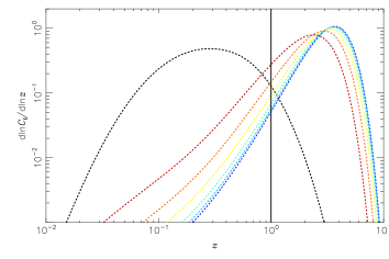
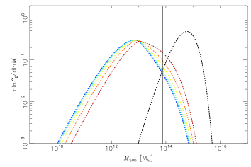
Figure 3: Top: predicted distribution of the tSZ and CIB power as a function of the redshift at $\ell=1000$. Bottom: predicted distribution of the tSZ and CIB power as a function of the host halo mass at $\ell=1000$. The black dashed line is for the tSZ effect, while the dark blue, light blue, green, yellow, orange, and red dashed lines are for CIB at 100, 143, 217, 353, 545, and 857 GHz respectively. The vertical solid black line shows the maximum redshift in PSZ2 (top panel) and the minimal $M_{500}$ in PSZ (bottom panel).

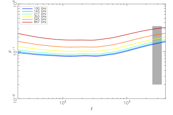
Figure 4: Predicted correlation factor of the tSZ-CIB cross-spectrum from 100 to 857 GHz. The grey shaded area represents the range of values predicted for $\rho$ from Zahn et al. (2012) for various models at 95, 150, and 220 GHz.

2.4 Predicted tSZ-CIB angular cross-power spectrum

In Fig. 2 we present the predicted tSZ-CIB angular cross-power spectra from 100 to 857 GHz, for the fiducial cosmological model and scaling-relation parameters listed in Table 1. The tSZ angular auto-spectrum is dominated by the 1-halo term, while the CIB auto-spectrum is dominated by the 2-halo-term up to $\ell\simeq 2000$. Thus we need to consider both contributions for the total cross-power spectrum.

At low $\ell$, we observe that the 2-halo term has a similar amplitude to the 1-halo term at all frequencies. The 1-halo term completely dominates the total angular cross-power spectrum up to $\ell\simeq 2000$. We also notice that the cross-power spectrum is highly sensitive to the parameters $\delta_{\rm CIB}$ and $\epsilon_{\rm CIB}$. Indeed, these two parameters set the overlap of the tSZ and CIB window functions in mass and redshift. Similarly, the relative amplitude of the 1-halo and 2-halo term is directly set by these parameters.

In Fig. 3, we present the redshift and mass distribution of tSZ and CIB power. These distributions are different for different multipoles. Given the angular scale probed by Planck, we show them for the specific multipole $\ell=1000$. We notice that the correlation between tSZ and CIB, at a given frequency, is determined by the overlap of these distributions. Clusters that constitute the main contribution to the total tSZ power are at low redshifts ($z<1$). The galaxies that produce the CIB are at higher redshifts ($1<z<4$). The mass distribution of CIB power peaks near $M_{500}=10^{13}\thinspace{\rm M_{\odot}}$, while the tSZ effect is produced mostly by halos in the range $10^{14}\thinspace{\rm M_{\odot}}<M_{500}<10^{15}\thinspace{\rm M_{\odot}}$.

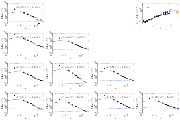
Figure 5: Upper right panel: observed tSZ power spectrum: Planck data from Planck Collaboration XXI (2014) (black symbols), ACT data (Reichardt et al. 2012) (light blue symbols), and SPT data (Sievers et al. 2013) (orange symbols); with our fiducial model (dashed blue line). Other panels: observed CIB power spectra, with Planck data from Planck Collaboration XXX (2014) (black) and our fiducial model (dashed blue line). These panels show auto- and cross-power spectra at 217, 353, 545, and 857 GHz. The dotted blue lines show the 1-halo plus shot-noise term for our fiducial model.

We define the correlation factor between tSZ and CIB signals, $\rho$, as

$$\rho=\frac{C_{\ell}^{{\rm tSZ-CIB}}}{\left(C_{\ell}^{\rm tSZ-tSZ}C_{\ell}^{\rm CIB-CIB}\right)^{1/2}}.$$ (13)

Figure 4 shows that we derive a correlation factor ranging from 0.05 to 0.30 at Planck frequencies. This agrees with the values reported from other tSZ-CIB modelling in the literature (Zahn et al. 2012; Addison et al. 2012), ranging from 0.02 to 0.34 at 95, 150, and 220 GHz. The difference in redshift and mass distributions of tSZ and CIB signals explains this relatively low degree of correlation.

We also observe that the tSZ-CIB correlation has a minimum around $\ell=300$, and significantly increases at higher multipoles. At those multipoles, the tSZ effect is dominated by low-mass and higher-redshift objects, overlapping better with the CIB range of masses and redshifts, which explains the increase of the correlation factor. The frequency dependence of the tSZ-CIB correlation factor can be explained by the variation of the CIB window in redshift as a function of frequency. At high frequencies, we observe low-redshift objects (with respect to other frequencies, but high-redshift objects from a tSZ perspective). On the other hand, at low frequencies, we are sensitive to higher redshift, as shown in Fig. 3.

2.5 Comparison with tSZ and CIB auto-spectra

We fixed $T_{{\rm d}0}$, $\alpha_{\rm CIB}$, $\beta_{\rm CIB}$, $\gamma_{\rm CIB}$, and $\delta_{\rm CIB}$ to the values from Planck Collaboration XXX (2014). We fix $\epsilon_{\rm CIB}$ to a value of 1.0, and we fit for $L_{0}$ in the multipole range $100<\ell<1000$ using CIB spectra from 217 to 857 GHz. We notice that the value of $\epsilon_{\rm CIB}$ is closely related to halo occupation distribution power-law index and highly degenerate with $\Omega_{\rm m}$.

In Fig. 5, we compare our modelling of the tSZ and CIB spectra with measured spectra from the Planck tSZ analysis (Planck Collaboration XXII 2015) and Planck data at 217, 353, 545, and 857 GHz (Planck Collaboration XXX 2014). For more details of these measurements see the related Planck papers referenced in Planck Collaboration I (2014) and Planck Collaboration I (2015). Here, we used the Planck-SZ best-fit cosmology presented in Table 1. We observe that our model reproduces the observed auto-power spectra for both tSZ and CIB anisotropies, except at low $\ell$ (below 100), where the CIB power spectra are still contaminated by foreground Galactic emission. For this reason, in this $\ell$ range the measured CIB power spectra have to be considered as upper limits. The figures show the consistency of the present CIB modelling at cluster scale with the modelling presented in Planck Collaboration XXX (2014) in the multipole range covered by the Planck data. Note that the flatness of the 1-halo term for CIB spectra ensures that this term encompasses the shot-noise part.

3 The data

3.1 Planck frequency maps

In this analysis, we use the Planck full-mission data set (Planck Collaboration I 2015; Planck Collaboration VIII 2015). We consider intensity maps at frequencies from 30 to 857 GHz, with 1$\aas@@fstack{\prime}$7 pixels, to appropriately sample the resolution of the higher-frequency maps. For the tSZ transmission in Planck spectral bandpasses, we use the values provided in Planck Collaboration IX (2014). We also used the bandpasses from Planck Collaboration IX (2014) to compute the CIB transmission in Planck channels for the SED. For power spectra analyses, we use Planck beams from Planck Collaboration IV (2015) and Planck Collaboration VII (2014).

3.2 The Planck SZ sample

In order to extract the tSZ-CIB cross-correlation, we search for infrared emission in the direction of clusters detected through their tSZ signal. In this analysis, we use galaxy clusters from the Planck SZ catalogue (Planck Collaboration XXVII 2015, PSZ2 hereafter) that have measured redshifts. We restrict our analysis to the sample of confirmed clusters to avoid contamination by false detections (see Aghanim et al. 2014, for more details). This leads to a sample of 1093 galaxy clusters with a mean redshift $\bar{z}\simeq 0.25$.

From this sample of clusters, we have built a reprojected tSZ map. We use a pressure profile from Arnaud et al. (2010), with the scaling relation presented in Planck Collaboration XX (2014), as well as the size ($\theta_{500}$) and flux ($Y_{500}$) computed from the 2-D posterior distributions delivered in Planck Collaboration XXVII (2015). We project each cluster onto an oversampled grid with a pixel size of $0.1\times\theta_{500}$ (using drizzling to avoid flux loss during the projection). Then we convolve the oversampled map with a beam of 10^′ FWHM. We reproject the oversampled map onto a HEALPix (Górski et al. 2005) full-sky map with 1$\aas@@fstack{\prime}$7 pixels ($N_{\rm side}=2048$) using nearest-neighbour interpolation.

3.3 IRAS data

We use the reprocessed IRAS maps, IRIS (Improved Reprocessing of the IRAS Survey, Miville-Deschênes & Lagache 2005) in the HEALPix pixelization scheme. These offer improved calibration, zero level estimation, zodiacal light subtraction, and destriping of the IRAS data. The IRIS 100, 60, and 25 $\mu$m maps are used at their original resolution. Missing pixels in the IRIS maps have been set to zero for this analysis.

4 Results for tSZ-detected galaxy clusters.

In this section, we present a detection of the tSZ-CIB cross-correlation using known galaxy clusters detected via the tSZ effect in the Planck data. In Sect. 4.1, we focus on the study of the shape and the SED of the infrared emission towards galaxy clusters. Then Sect. 4.2 is dedicated to the study of the tSZ-CIB cross-power spectrum for confirmed tSZ clusters.

4.1 Infrared emission from clusters

4.1.1 Stacking of Planck frequency maps

To increase the significance of the detection of infrared emission at galaxy-cluster scales, we perform a stacking analysis of the sample of SZ clusters defined in Sect. 3. Following the methods presented in Hurier et al. (2014), we extract individual patches of $4^{\circ}\times 4^{\circ}$ from the full-sky Planck intensity maps and IRIS maps centred at the position of each cluster. The individual patches are re-projected using a nearest-neighbour interpolation on a grid of 0$\aas@@fstack{\prime}$2 pixels in gnomonic projection to conserves the cluster flux. We then produce one stacked patch for each frequency. To do so, the individual patches per frequency are co-added with a constant weight. This choice accounts for the fact that the main contribution to the noise, i.e., the CMB, is similar from one patch to another. Furthermore, it avoids cases where a particular cluster dominates the stacked signal. Considering that Galactic thermal dust emission is not correlated with extragalactic objects, emission from our Galaxy should not bias our stacking analysis. We verified that the stacking is not sensitive to specific orientations, which may be produced by the thermal dust emission from the Galactic plane. We produced a stacked patch per frequency for the whole cluster sample, and for two large redshift bins (below and above $z=0.15$).

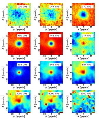
Figure 6: From left to right and top to bottom: observed stacked intensity maps at 30, 44, 70, 100, 143, 217, 353, 545, 857, 3000, 5000, and 12 000 GHz at the positions of confirmed SZ clusters. All maps are at the native angular resolution of the relevant Planck channel. The measured intensity increases from dark blue to red.

In Fig. 6, we present the stacked signal at the positions of the sample of confirmed SZ clusters in Planck data from 30 to 857 GHz and in IRIS maps from 100 to 25 $\mu$m. At low frequencies (below 217 GHz) we observe the typical tSZ intensity decrement. However, at 353 and 545 GHz we see a mix of the positive tSZ signal and infrared emission. We also note that the infrared emission can also be observed at 217 GHz where the tSZ effect is negligible. We note the presence of significant infrared emission in the Planck 857 GHz channel, where the tSZ signal is negligible. Similarly we find a significant infrared signal in the IRAS 100 and 60 $\mu$m bands.

4.1.2 The SED of galaxy clusters

Each stacked map from 70 GHz upwards is created at a resolution of ${\rm FWHM}=13{{}^{\scriptstyle\prime}}$. We measure the flux, $F(\nu)$, in the stacked patches from 30 to 853 GHz through aperture photometry within a radius of 20^′ and compute the mean signal in annuli ranging from 30^′ to 60^′ to estimate the surrounding background level. We use aperture photometry in order to obtain a model-independent estimation of the total flux, without assuming a particular shape for the galaxy cluster profile. Thus, the flux is computed as

$$\widehat{F}(\nu)=K_{\nu}\left(\sum_{r<20{{}^{\scriptstyle\prime}}}A_{\nu,p}-\sum_{{30{{}^{\scriptstyle\prime}}}<r<60{{}^{\scriptstyle\prime}}}A_{\nu,p}\frac{N_{r<20{{}^{\scriptstyle\prime}}}}{N_{{30{{}^{\scriptstyle\prime}}}<r<60{{}^{\scriptstyle\prime}}}}\right)\Delta\Omega,$$ (14)

where $A_{\nu,p}$ is the pixel $p$ separated from the centre of the map by a distance $r$ in the stacked map $A_{\nu}$, $\Delta\Omega$ is the solid angle of one pixel, $N_{X}$ is the number of pixels that follow the condition $X$, and $K_{\nu}$ is the bias for the aperture photometry (equal to one except at 30 and 44 GHz). The 30 and 44 GHz channels have a lower angular resolution and thus the aperture photometry does not measure all the signal. We compute the factor $K_{\nu}$ by assuming that the physical signal at 143 GHz has the same spatial distribution as that at 30 or 44 GHz:

$$K_{\nu}=\frac{\widehat{F}(143)}{\widehat{F}^{*}(143,\nu)},$$ (15)

where the flux $\widehat{F}^{*}(143,\nu)$, is computed on the 143  GHz stacked map after being set to the resolution of the 30 and 44 GHz channels.

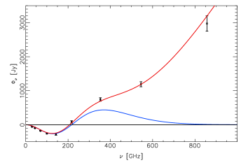
Figure 7: Observed SED of the stacked signal towards galaxy clusters, from 30 to 857 GHz. In blue we show the tSZ contribution to the total SED and in red the total SED considering infrared emission.

From the scaling laws presented in Sect. 2, it is possible to predict the expected SED of a cluster. The total tSZ plus infrared emission measured through stacking of $N_{\rm cl}$ clusters can be written as

$$F(\nu)=\sum_{i}^{N_{\rm cl}}\left[g(\nu)Y^{i}_{500}+S^{i}_{500}(\nu)\right],$$ (16)

where ${S}_{500}(\nu)=a\thinspace L_{500}(\nu)/4\pi\chi^{2}(z)$ is based on values from Table 1 and we fit for $L_{0}$ (see Eq. 6 for the $L_{500}$ expression), which sets the global amplitude of the infrared emission in clusters.

Figure 7 presents the derived SED towards galaxy clusters compared to the tSZ-only SED. The observed flux at high frequencies, from 353 to 857 GHz, calls for an extra infrared component to account for the observed emission. We also present in Fig. 8 the same SED for two wide redshift bins, below and above $z=0.15$, with median redshift $0.12$ and $0.34$, respectively. We observe that most of the infrared emission is produced by objects at $z>0.15$. We compare this stacking analysis to the SED prediction from the scaling relation used to reproduce results presented in Fig. 7 (red lines). This shows that the modelling reproduces the observed redshift dependence of the infrared flux of galaxy clusters.

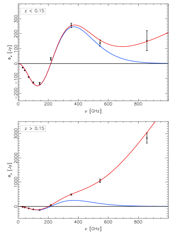
Figure 8: Observed SED of the stacked signal toward galaxy clusters, from 30 to 857 GHz. Top: objects below $z=0.15$. Bottom: objects above $z=0.15$. In blue we show the tSZ contribution to the total SED and in red the total SED considering infrared emission.

Uncertainties on $\widehat{F}(\nu)$ are mainly produced by contamination from other astrophysical components. To estimate the induced contamination level, we extract fluxes, $F^{\prime}_{\nu,q}$, at 1000 random positions, $q$, across the sky with the same aperture photometry as the one presented in Sect. 4.1.2. To derive a realistic estimation of the noise, we avoid the Galactic plane area for the random positions, since this area is not represented in our cluster sample (for details of the sky coverage of the PSZ1 and PSZ2 catalogues see Planck Collaboration XXIX 2014 and Planck Collaboration XXVII 2015). In the stacking process each cluster is considered uncorrelated with the others. Indeed, considering the small number of objects, we can safely neglect correlations induced by clustering in the galaxy cluster distribution. The $F_{\nu}$ uncertainty correlation matrix is presented in Fig. 9. It only accounts for uncertainties produced by uncorrelated components (with respect to the tSZ effect) in the flux estimation. From 44 to 217 GHz, the CMB anisotropies are the main source of uncertainties. This explains the high level of correlation in the estimated fluxes. The 30 GHz channel has a lower level of correlation due to its high noise level. At higher frequencies, from 353 to 857 GHz, dust residuals becomes the dominant source in the total uncertainty, which explains the low level of correlation with low frequency channels. Contamination by radio sources inside galaxy clusters can be neglected (at least statistically), since the measured fluxes at 30 and 44 GHz agree with the tSZ SED.

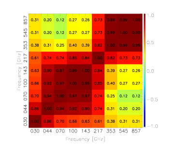
Figure 9: Correlation matrix of ${\widehat{F}}(\nu)$ estimated from 1000 random positions across the sky.

4.1.3 Comparison between tSZ, IR, and galaxy-number radial profiles

We computed the radial profile of each stack map from 70 to 857 GHz in native angular resolution.These profiles were calculated on a regular radial grid of annuli with bins of width $\Delta r=1{{}^{\scriptstyle\prime}}$, allowing us to sample the stacked map at a resolution similar to the Planck pixel size. The profile value in a bin is defined as the mean of the values of all pixels falling in each annulus. We subtract a background offset from the maps prior to the profile computation. The offset value is estimated from the surrounding region of each cluster ($30{{}^{\scriptstyle\prime}}<r<60{{}^{\scriptstyle\prime}}$). The uncertainty associated with this baseline offset subtraction is propagated into the uncertainty of each bin of the radial profile.

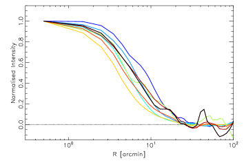
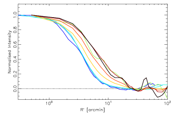
Figure 10: Top: observed radial profile of the stacked signal toward galaxy clusters at the native angular resolution at 70 GHz (in dark blue), 100 GHz (blue), 143 GHz (light blue), 217 GHz (green), 353 GHz (orange), 545 GHz (red), 857 GHz (dark red), and 100 $\mu$m (black). Bottom: same as top panel, but as a function of the rescaled radius $R{{}^{\scriptstyle\prime}}=R({\cal B}_{\nu}/{\cal B}_{857})$.

In Fig. 10, we present the profile normalized to one at the centre. We observe that profiles derived from low-frequency maps show a larger extension due to beam dilution. The smallest extension of the signal is obtained for 353 GHz, then it increases with frequency. For comparison we also display the profile at 100 $\mu$m, which shows the same extension as the profiles at 217 and 857 GHz where there is no significant tSZ emission. For illustration, in the bottom panel of Fig. 10, we display the profiles as a function of the rescaled radius $R{{}^{\scriptstyle\prime}}=R({\cal B}_{\nu}/{\cal B}_{857})$, with ${\cal B}_{\nu}$ the FWHM of the beam at frequency $\nu$. Under the assumption that the tSZ profile is Gaussian, this figure allows us to directly compare the extension of the signal at all frequencies; it illustrates the increase of the signal extension with frequency, except for the 217 GHz profiles, which have the same size as the high-frequency profiles.

We then define the extension of the Planck profiles as ${\cal E}(\nu)$, where

$${\cal E}^{2}(\nu)=4\pi\thinspace\ln 2\left(\frac{\int rp(r,\nu){\rm d}r}{\int p(r,\nu){\rm d}r}\right)^{2}-{\cal B}^{2}_{\nu},$$ (17)

with $p(r,\nu)$ the profile of the stacked signal at frequency $\nu$. Integration of the profiles is performed up to $r=30{{}^{\scriptstyle\prime}}$. The quantity ${\cal E}(\nu)$ is equivalent to a FWHM for a Gaussian profile; however, we notice that the profile of the stacked signal deviates from a Gaussian at large radii. This increases the values obtained for the profile extension. We estimate the uncertainty on the profile extension using 1000 random positions on the sky.

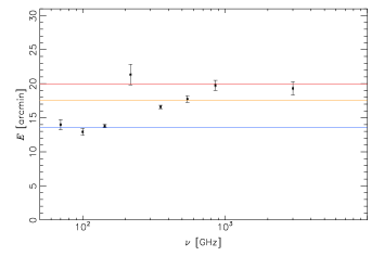
Figure 11: Variation of the spatial extension, ${\cal E}(\nu)$, of the stacked signal from 70 to 3000 GHz (100$\thinspace\mu$m). The blue line shows the expected value for the GNFW profile from Arnaud et al. (2010) and $\theta_{500}$ values from PSZ1, the orange line shows the value we derive with the Xia et al. (2012) profile, and the red line shows the value for an NFW profile with $c_{500}=1.0$.

In Fig. 11, we present the variation of ${\cal E}(\nu)$ as a function of frequency from 70 GHz to 3000 GHz (100$\thinspace\mu$m). We see lower values of ${\cal E}(\nu)$ at low frequencies. The observed signal is composed of two separate components, the tSZ effect and the infrared emission from clusters. The variation of ${\cal E}(\nu)$ is produced by the difference between the spatial extension of the tSZ effect and the infrared emission. At frequencies dominated by the tSZ signal (from 70 to 143 GHz), we observe ${\cal E}(\nu)=13\aas@@fstack{\prime}6\pm 0\aas@@fstack{\prime}1$. The expected value for the Arnaud et al. (2010) GNFW profile and $\theta_{500}$ values for the Planck clusters is ${\cal E}(\nu)=13\aas@@fstack{\prime}6$. We observe ${\cal E}(\nu)=20\aas@@fstack{\prime}0\pm 0\aas@@fstack{\prime}5$ at 217, 857, and 3000 GHz. At 217 GHz, where the tSZ signal is almost null, ${\cal E}(\nu)$ is dominated by the infrared emission and is similar to the signal found at high frequencies (857 GHz and 100 $\mu$m). Considering an NFW profile for infrared emission,

$$p(r)\propto\frac{1}{\left(c_{500}\frac{r}{R_{500}}\right)\left(1+c_{500}\frac{r}{R_{500}}\right)^{2}},$$ (18)

and $\theta_{500}$ values for the Planck clusters, the previous result translates into constraints on $c_{500}$, giving $c_{500}=1.00^{+0.18}_{-0.15}$. For comparison, we also display in Fig. 11 the prediction based on the profile used in Xia et al. (2012), which assumes a concentration

$$c_{\rm vir}=\frac{9}{1+z}\left(\frac{M}{M_{*}}\right)^{-0.13},$$ (19)

where $M_{*}$ is the mass for which $\nu(M,z)=\delta_{\rm c}/\left(D_{\rm g}\sigma(M)\right)$ is equal to 1 (Bullock et al. 2001), with $\delta_{\rm c}$ the critical over-density, $D_{\rm g}$ the linear growth factor, and $\sigma(M)$ the present-day rms mass fluctuation.

This model leads to ${\cal E}(\nu)=17\aas@@fstack{\prime}6$. As a consequence, our results demonstrate that galaxies in the outskirts of clusters give a larger contribution to the total infrared flux than galaxies in the cluster cores. Indeed, star formation in outlying galaxies is not yet completely quenched, while galaxies in the core no longer have a significant star formation rate. This result is consistent with previous analyses that found radial dependence for star-forming galaxies (e.g., Weinmann et al. 2010; Braglia et al. 2011; Coppin et al. 2011; Santos et al. 2013; Muzzin et al. 2014).

We also model the radial dependence of the average specific star-formation rate (SSFR) as $\left[1-A_{\rm q}{\rm exp}\left(-\alpha_{\rm q}r/R_{500}\right)\right]$, where $1-A_{\rm q}$ is the ratio between the SSFR of a core galaxy and an outlying galaxy and $\alpha_{\rm q}$ is the radial dependence of the infrared emission suppression. We adopt the profile from Xia et al. (2012) for the galaxy distribution and, using $A_{\rm q}\simeq 0.7$, we derive $\alpha_{\rm q}=0.5^{+0.5}_{-0.2}$.

4.2 Cross-correlation between the tSZ catalogue and temperature maps

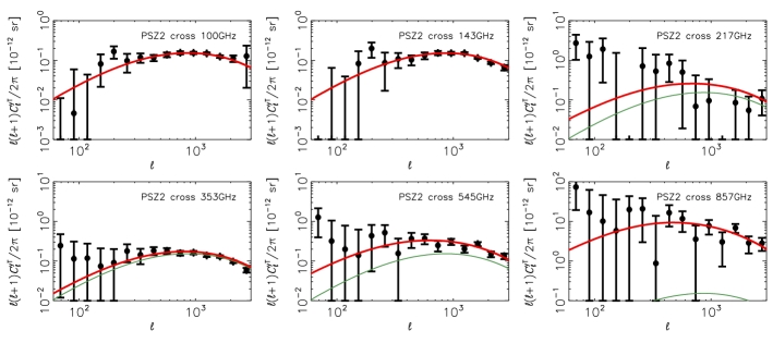
Figure 12: Observed cross-correlation between the tSZ map ($y_{\rm c}$) of known clusters and the Planck frequency maps ($T_{\nu}$), from 100 to 857 GHz. The data are presented as black circles, the tSZ auto-correlation is in green and the total model $y_{\rm c}$–$T_{\nu}$ accounting for tSZ-CIB correlation is in red for the best-fit of the CIB and tSZ spectra. All power spectra are presented in Compton-parameter units. Uncertainties are dominated by foreground residuals; thus they are highly correlated from one channel to another.

4.2.1 Methodology

We focus on the detection of the correlation between tSZ and infrared emission at the positions of confirmed galaxy clusters. To do so, we use a map constructed from the projection of confirmed SZ clusters on the sky, hereafter called the “reprojected tSZ map,” (see end of Sect. 3.2). We measure the tSZ-CIB cross-correlation by computing the angular cross-power spectrum, $C_{\ell}^{y_{\rm c}T_{\nu}}$, between the reprojected tSZ map, $y_{\rm c}$, and the Planck intensity maps, $T_{\nu}$, from 100 GHz to 857 GHz. We note that $y_{\rm c}$ is only a fraction of the total tSZ emission of the sky, $y$. The cross-spectra are

$$C_{\ell}^{y_{\rm c}T_{\nu}}=g(\nu)C_{\ell}^{y_{\rm c},y}+C_{\ell}^{y_{\rm c},{\rm CIB}(\nu)},$$ (20)

where $C_{\ell}^{y_{\rm c},{\rm CIB}(\nu)}$ is the cross-correlation between the reprojected tSZ map (in Compton parameter units) and the CIB at frequency $\nu$. Considering that the tSZ power spectrum is dominated by the 1-halo term, we have $C_{\ell}^{y_{\rm c},y}\simeq C_{\ell}^{y_{\rm c},y_{\rm c}}$. We mask the thermal dust emission from the Galaxy, keeping only the cleanest 40 % of the sky. This mask is computed by thresholding the 857 GHz Planck full sky map at 30^′ FWHM resolution. We verified that we derive compatible results with 30 and 50 % of the sky. We bin the cross-power spectra and correct them for the beam and mask effects. In practice, the mixing between multipoles induced by the mask is corrected by inverting the mixing matrix $\@tens{M}_{bb}$ between bins of multipoles (see Tristram et al. 2005).

We estimate the uncertainties on the tSZ-CIB cross-spectra as

$$\left(\Delta C_{\ell}^{y_{\rm c}T_{\nu}}\right)^{2}=\frac{1}{(2\ell+1)f_{\rm sky}}\left[\left(C_{\ell}^{y_{\rm c}T_{\nu}}\right)^{2}+C_{\ell}^{y_{\rm c}y_{\rm c}}C_{\ell}^{T_{\nu}T_{\nu}}\right].$$ (21)

We stress that due to cosmic variance the uncertainties on the $C_{\ell}^{y_{\rm c}T_{\nu}}$ spectra are highly correlated from frequency to frequency. We see in Fig. 12 that cross-spectra at different frequencies show similar features. The covariance matrix between cross-spectra at frequencies $\nu$ and $\nu^{\prime}$ can be expressed as

$${\rm cov}\left(C_{\ell}^{y_{\rm c}T_{\nu}},C_{\ell}^{y_{\rm c}T_{\nu^{\prime}}}\right)=\frac{1}{(2\ell+1)f_{\rm sky}}\left[C_{\ell}^{y_{\rm c}T_{\nu}}C_{\ell}^{y_{\rm c}T_{\nu^{\prime}}}+C_{\ell}^{y_{\rm c}y_{\rm c}}C_{\ell}^{T_{\nu}T_{\nu^{\prime}}}\right].$$ (22)

Then we propagate the uncertainties through the bins and the mixing matrix $\@tens{M}^{-1}_{bb}$. We verify using Monte Carlo simulations that we derive compatible levels of uncertainty. In the following analysis, we use the full covariance matrix between multipole bins.

We also consider uncertainties produced by the Planck bandpasses (Planck Collaboration IX 2014). This source of uncertainty reaches up to 20 % for the tSZ transmission at 217 GHz. We also account for relative calibration uncertainties (Planck Collaboration VIII 2015) ranging from 0.1 % to 5 % for different frequencies. We verify that our methodology is not biased by systematic effects by cross-correlating Planck intensity maps with nominal cluster centres randomly placed on the sky, and we observe a cross-correlation signal compatible with zero.

4.2.2 Results

In Fig. 12, we present the measured angular cross-power spectra and our fiducial model. For convenience, all spectra are displayed in Compton-parameter units; as a consequence the tSZ auto-correlation has the same amplitude at all frequencies. We note that at 217 GHz the tSZ transmission is very faint. Thus, it induces large uncertainties when displayed in Compton-parameter units; at this specific frequency, the cross-power spectrum is dominated by the tSZ-CIB contribution, since the CIB emission dominates over the tSZ emission at 217 GHz ($g(\nu)$ becomes negligible in Eq. 20). Uncertainties are highly correlated from one channel to another, explaining the similar features we observed in the noise at all frequencies.

In order to address the significance of the tSZ-CIB correlation in the measured cross-spectra we consider three cases to describe the angular cross-power spectra and we compute the $\chi^{2}$ for each case and each frequency:

• in Case 1, no tSZ auto-correlation and no tSZ-CIB correlation;

• in Case 2, only a tSZ auto-correlation contribution;

• in Case 3, both tSZ and tSZ-CIB spectra.

We present the derived $\chi^{2}$ values in Table 2.

At low frequencies, 100 and 143 GHz, the measured signal is completely dominated by the tSZ auto-spectrum. The consistency between the observed spectrum and the predicted one demonstrates that fluxes from the Planck SZ clusters are consistent with our measurement. At intermediate multipoles the tSZ-CIB contribution has a similar amplitude to the contribution of tSZ auto-spectra. At 217 and 353 GHz we observe a higher value for the $\chi^{2}$ in Case 3 compared to the value for in Case 2. However, the difference between these values is not significant, considering the number of degree of freedom per spectra. Thus the tSZ-CIB contribution is not significant for these frequencies. However, at 545 and 857 GHz we detect a significant excess with respect to the tSZ auto-correlation contribution. We detect the tSZ-CIB contribution for low-redshift objects at 5.8 and 6.0$\thinspace\sigma$ at 545 and 857 GHz, respectively.

Table 2: Value of $\chi^{2}$ for the $y$–$T_{\nu}$ spectra from 100 to 857 GHz (presented in Fig. 12) coming from a null test (Case 1), using only the tSZ spectra (Case 2), and when considering both tSZ and tSZ–CIB spectra (Case 3). The adjustment is performed in the multipole range $200>\ell>2500$ with 60 degrees of freedom (approximately 10 degrees of freedom per frequency). Thus each $\chi^{2}$ value should be considered to be associated with $N_{\rm dof}\simeq 10$.

$$\nu$$ [GHz]

100 143 217 353 545 857

Case 1. 600.0 617.3 7.9 368.2 172.0 45.0

Case 2. 4.5 8.3 6.8 6.6 41.1 43.1

Case 3. 4.5 7.8 9.1 8.0 6.9 7.0

5 The total tSZ-CIB cross-correlation

In this section we investigate the all-sky tSZ-CIB cross-correlation using two different approaches: (i) the tSZ-CIB cross-power using a tSZ Compton-parameter map (Sect. 5.1); and (ii) the tSZ-CIB cross-power from a study of cross-spectra between Planck frequencies (Sect  5.2).

5.1 Constraints on the tSZ-CIB cross-correlation from tSZ $y$-map/frequency maps cross-spectra

This section presents the tSZ-CIB estimation using the cross-correlation between a Planck tSZ map and Planck frequency maps. Since the tSZ map contains CIB residuals, we carefully modelled these residuals in order to estimate the contribution from the tSZ-CIB correlations.

5.1.1 Methodology

We compute the cross-power spectra between the Planck frequency maps and a reconstructed $y$-map derived from component separation (see Planck Collaboration XXII 2015, and references therein). We choose the MILCA map and check that there are no significant differences with the NILC map (both maps are described in Planck Collaboration XXII 2015). This cross-correlation can be decomposed into four terms:

$$C_{\ell}^{\widehat{y},T_{\nu}}=g(\nu)C_{\ell}^{y,y}+C_{\ell}^{y,{\rm CIB}(\nu)}+g(\nu)C_{\ell}^{y,y_{\rm CIB}}+C_{\ell}^{y_{\rm CIB},{\rm CIB}(\nu)},$$ (23)

where $y_{\rm CIB}$ is the CIB contamination in the tSZ map. We compute the uncertainties as

$${\rm cov}(C_{\ell}^{\widehat{y},T_{\nu}},C_{\ell}^{\widehat{y},T_{\nu}^{\prime}})=\frac{C_{\ell}^{\widehat{y},\widehat{y}}C_{\ell}^{T_{\nu},T_{\nu}^{\prime}}+C_{\ell}^{\widehat{y},T_{\nu}}C_{\ell}^{\widehat{y},T_{\nu}^{\prime}}}{(2\ell+1)f_{\rm sky}},$$ (24)

where $f_{\rm sky}$ is the fraction of the sky that is unmasked. We bin the cross-power spectrum and deconvolve the beam and mask effects, then we propagate uncertainties as described in Sect. 4.2.

The cross-correlations of a tSZ-map built from component-separation algorithms and Planck frequency maps are sensitive to both the tSZ auto-correlation and tSZ-CIB cross-correlation. But this cross-correlation also has a contribution produced by the CIB contamination to the tSZ map. In particular, this contamination is, by construction, highly correlated with the CIB signal in the frequency maps.

5.1.2 Estimation of CIB leakage in the tSZ map

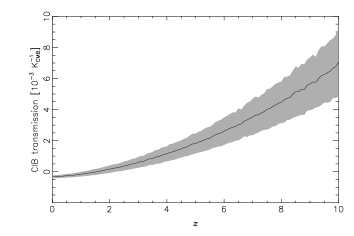
Figure 13: Predicted CIB transmission in the tSZ $y$-map for a hypothetical CIB emission of 1 K_CMB at 545 GHz and at redshift $z$. The shaded area represents the 68% confidence region, for uncertainties of $\Delta T_{\rm d}=2\thinspace$K and $\Delta\beta_{\rm d}=0.1$ in the modified blackbody parameters of the hypothetical CIB emission.

The tSZ maps, denoted $\widehat{y}$ in the following, are derived using component-separation methods. They are constructed through a linear combination of Planck frequency maps that depends on the angular scale and the pixel, $p$, as

$$\widehat{y}=\sum_{i,j,\nu}w_{i,p,\nu}T_{i,p}(\nu).$$ (25)

Here $T_{i,p}(\nu)$ is the Planck map at frequency $\nu$ for the angular filter $i$, and $w_{i,p,\nu}$ are the weights of the linear combination. Then, the CIB contamination in the $y$-map is

$$y_{\rm CIB}=\sum_{i,j,\nu}w_{i,p}(\nu)T^{\rm CIB}_{i,p}(\nu),$$ (26)

where $T^{\rm CIB}(\nu)$ is the CIB emission at frequency $\nu$. Using the weights $w_{i,p,\nu}$, and considering the CIB luminosity function, it is possible to predict the expected CIB leakage as a function of the redshift of the source by propagating the SED through the weights that are used to build the tSZ map.

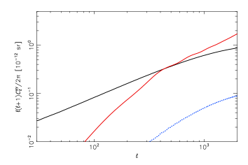
Figure 14: Expected contribution to the tSZ power spectrum for the true tSZ signal (black curve), for CIB leakage (red curve), and for tSZ-CIB leakage contribution (blue curve). The dotted line indicates a negative power spectrum.

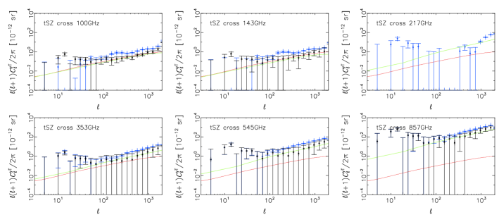
Figure 15: From left to right and top to bottom: observed cross-correlation between the MILCA $y$-map and the Planck frequency maps from 30 to 857 GHz. In blue are the data points, in black the CIB-cleaned data points; the red solid line is the predicted signal from tSZ only and the green line is the total expected signal from the tSZ signal and the tSZ-CIB correlation. All spectra are presented in Compton-parameter units.

In Fig. 13, we present the expected transmission of CIB emission in the Planck tSZ map for a $1\thinspace{\rm K}_{\rm CMB}$ CIB source at 545 GHz at redshift $z$, based on the fiducial model for the scaling relation presented in Sect. 2. The intensity of CIB leakage in the tSZ map is given by the integration of the product of CIB transmission (presented in Fig. 13) and the CIB scaling relation at 545 GHz. Error bars account for SED variation between sources. In this case we assume an uncertainty of $\Delta T_{\rm d}=2\thinspace$K and $\Delta\beta_{\rm d}=0.1$ on the modified blackbody parameters. We observe that the CIB at low $z$ leaks into the tSZ map with only a small amplitude, whereas higher-redshift CIB produces a higher, dominant, level of leakage. Indeed, ILC-based component-separation methods tend to focus on Galactic thermal dust removal, and thus are less efficient at subtracting high-$z$ CIB sources that have a different SED.

The CIB power spectra have been constrained in previous Planck analyses (see, e.g., Planck Collaboration XVIII 2011; Planck Collaboration XXX 2014), as presented in Sect. 2.5. We can use this knowledge of the CIB power spectra to predict the expected CIB leakage, $y_{\rm CIB}$, in the tSZ map, $y$. We performed 200 Monte Carlo simulations of tSZ and CIB maps that follow the tSZ, CIB, and tSZ-CIB power spectra. Then, we applied to these simulations the weights used to build the tSZ map. Finally, we estimated the CIB leakage and its correlation with the tSZ effect. The tSZ map signal, $\widehat{y}$, can be written as $\widehat{y}=y+y_{\rm CIB}$. Thus, the spectrum of the tSZ map is $C_{\ell}^{\widehat{y},\widehat{y}}=C_{\ell}^{y,y}+C_{\ell}^{y_{\rm CIB},y_{\rm CIB}}+2C_{\ell}^{y,y_{\rm CIB}}$.

In Fig. 14, we present the predicted contributions to the tSZ map’s power spectrum for tSZ, CIB leakage, and tSZ-CIB leakage. We observe that at low $\ell$ (below 400) the tSZ signal dominates CIB leakage and tSZ-CIB leakage contamination, whereas for higher $\ell$ the signal is dominated by the CIB leakage part. The tSZ-CIB leakage spectrum (dotted line in the figure) is negative, since it is dominated by low-$z$ ($z\la 2$) CIB leakage.

We also estimate the uncertainties on $C_{\ell}^{y_{\rm CIB},y_{\rm CIB}}$, using the uncertainty on the CIB correlation matrix from Planck Collaboration XXX (2014). We derive an average uncertainty of 50 % on the CIB leakage amplitude in the tSZ map. This uncertainty is correlated between multipoles at a level above 90 %. Consequently, the uncertainty on the CIB leakage in the tSZ-map can be modelled as an overall amplitude factor.

5.1.3 Results

By cross-correlating the simulated CIB leakage signal with the simulated CIB at each frequency, it is also possible to predict the CIB leakage in the cross-spectra between tSZ map and Planck frequency maps. We can correct $C_{\ell}^{\widehat{y},T_{\nu}}$ spectra (Eq. 23) using the estimated tSZ-CIB leakage cross-correlation term, $g(\nu)C_{\ell}^{y,y_{\rm CIB}}$, and the CIB-CIB leakage cross-correlation term, $C_{\ell}^{y_{\rm CIB},{\rm CIB}(\nu)}$, giving

$$C_{\ell}^{\widehat{y},T_{\nu},{\rm corr}}=C_{\ell}^{\widehat{y},T_{\nu}}-g(\nu)C_{\ell}^{y,y_{\rm CIB}}-C_{\ell}^{y_{\rm CIB},{\rm CIB}(\nu)}.$$ (27)

Thus, the only remaining contributions are from the tSZ auto-correlation and the tSZ-CIB cross-correlation. We also propagate the associated uncertainties.

Fig. 15 shows the cross-correlation of the tSZ-map and Planck frequency maps after correcting for the effects of the beam and mask, and for the terms $g(\nu)C_{\ell}^{y,y_{\rm CIB}}$ and $C_{\ell}^{y_{\rm CIB},{\rm CIB}(\nu)}$. As was the case for Fig. 12, all spectra are displayed in tSZ Compton-parameter units, and the uncertainties present a high degree of correlation from one frequency to another. For each cross-spectrum we adjust the amplitude, $A_{\rm tSZ-CIB}$, of the tSZ-CIB contribution through a linear fit. The results of the fit are listed in Table 3. We obtain a maximum significance of 2.3$\thinspace\sigma$ at 857 GHz and the results are consistent with the fiducial model.

Table 3: Best-fit values for the tSZ–CIB amplitude, $A_{\rm tSZ-CIB}$, using the fiducial model as reference.

$$\nu A_{\rm tSZ-CIB} \Delta A_{\rm tSZ-CIB} -3.6 3.8 -1.6 3.7 \kern 6.22224pt2.0 2.0 \kern 6.22224pt1.7 1.4 \kern 6.22224pt1.6 0.7$$ [GHz] 100. 143. 353. 545. 857.

The combined constraints from 353, 545, and 857 GHz measurements, as well as the covariance structure of the measurement uncertainties, yield an estimate of $A_{\rm tSZ-CIB}=1.3\pm 0.4$. The uncertainties are dominated by CIB leakage subtraction, which leads to highly correlated uncertainties of the 353, 545, and 857 GHz spectra. The optimal linear estimator we use to calculate $A_{\rm tSZ-CIB}$ probes the measurements for the known frequency trend of the CIB leakage in order to correct for this. Since the CIB leakage has affected all three of these correlated measurements in the same direction, the combined constraint of $1.3\pm 0.4$ is below the range of the individual (uncorrected) constraints ranging from 1.6 to 2.0. Table 3 contains the necessary covariance information used here.

5.2 Constraints on tSZ-CIB cross-correlation from Planck frequency maps

As a last approach, we explore the direct cross-correlation between Planck frequency maps.

5.2.1 Methodology

In terms of tSZ and CIB components the cross-spectra between frequencies $\nu$ and $\nu^{\prime}$ can be written as

$$C_{\ell}^{\nu,\nu^{\prime}}= \thinspace g(\nu)g(\nu^{\prime})C^{\rm y,y}_{\ell}+C_{\ell}^{\rm CIB(\nu),CIB(\nu^{\prime})}+g(\nu)C_{\ell}^{\rm y,CIB(\nu^{\prime})}$$

$$+g(\nu^{\prime})C_{\ell}^{\rm y,CIB(\nu)}+C_{\ell}^{\rm other}(\nu),$$ (28)

where $C_{\ell}^{\rm other}(\nu)$ accounts for the contribution of all components except for tSZ and CIB. We compute the cross-spectra between Planck frequency maps from 100 to 857 GHz as

$$C^{\nu,\nu^{\prime}}_{\ell}=\frac{C^{\nu_{1},\nu^{\prime}_{2}}_{\ell}+C^{\nu_{2},\nu^{\prime}_{1}}_{\ell}}{2},$$ (29)

where subscripts $1$ and $2$ label the “half-ring” Planck maps. This process allows us to produce power spectra without the noise contribution. We also compute the covariance between spectra as

$${\rm cov}(C^{\nu,\nu^{\prime}}_{\ell},C^{\nu^{\prime\prime},\nu^{\prime\prime\prime}}_{\ell}) =\frac{C^{\nu_{1},\nu^{\prime\prime}_{1}}_{\ell}C^{\nu^{\prime}_{2},\nu^{\prime\prime\prime}_{2}}_{\ell}+C^{\nu_{1},\nu^{\prime\prime\prime}_{2}}_{\ell}C^{\nu^{\prime}_{2},\nu^{\prime\prime}_{1}}_{\ell}}{4(2\ell+1)f_{\rm sky}}$$

$$+\frac{C^{\nu_{1},\nu^{\prime\prime}_{2}}_{\ell}C^{\nu^{\prime}_{2},\nu^{\prime\prime\prime}_{1}}_{\ell}+C^{\nu_{1},\nu^{\prime\prime\prime}_{1}}_{\ell}C^{\nu^{\prime}_{2},\nu^{\prime\prime}_{2}}_{\ell}}{4(2\ell+1)f_{\rm sky}}$$

$$+\frac{C^{\nu_{2},\nu^{\prime\prime}_{1}}_{\ell}C^{\nu^{\prime}_{1},\nu^{\prime\prime\prime}_{2}}_{\ell}+C^{\nu_{2},\nu^{\prime\prime\prime}_{2}}_{\ell}C^{\nu^{\prime}_{1},\nu^{\prime\prime}_{1}}_{\ell}}{4(2\ell+1)f_{\rm sky}}$$

$$+\frac{C^{\nu_{2},\nu^{\prime\prime}_{2}}_{\ell}C^{\nu^{\prime}_{1},\nu^{\prime\prime\prime}_{1}}_{\ell}+C^{\nu_{2},\nu^{\prime\prime\prime}_{1}}_{\ell}C^{\nu^{\prime}_{1},\nu^{\prime\prime}_{2}}_{\ell}}{4(2\ell+1)f_{\rm sky}}.$$ (30)

We correct the cross-spectra for beam and mask effects, using the same Galactic mask as in Sect. 4.2, removing 60 % of the sky, and we propagate uncertainties on cross-power spectra as described in Sect. 4.2.

The tSZ and CIB contributions to $C_{\ell}^{\nu,\nu^{\prime}}$ are contaminated by other astrophysical emission. We remove the CMB contribution in $C_{\ell}^{\nu,\nu^{\prime}}$ using the Planck best-fit cosmology (Planck Collaboration XIII 2015). We note that the Planck CMB maps suffer from tSZ and CIB residuals, so they cannot be used for our purpose.

5.2.2 Estimation of tSZ-CIB amplitude

We fit thermal dust, radio sources, tSZ, CIB (that accounts for the total fluctuations in extragalactic infrared emission), and tSZ-CIB amplitudes, $A_{\rm dust}$, $A_{\rm rad}$, $A_{\rm tSZ}$, $A_{\rm CIB}$, and $A_{\rm tSZ-CIB}$, respectively, through a linear fit. For the dust spectrum we assume $C_{\ell}\propto\ell^{\thinspace-2.8}$ (Planck Collaboration XXX 2014), and for radio sources $C_{\ell}\propto\ell^{\thinspace 0}$. For the tSZ-CIB correlation, tSZ, and CIB power spectra, we use templates computed as presented in Sect. 2.3. This gives us

$$C_{\ell}^{\nu,\nu^{\prime}} =A_{\rm tSZ}g(\nu)g(\nu^{\prime})C^{\rm y,y}_{\ell}$$

$$+A_{\rm CIB}C_{\ell}^{\rm CIB(\nu),CIB(\nu^{\prime})}$$

$$+A_{\rm tSZ-CIB}\left[g(\nu)C_{\ell}^{\rm y,CIB(\nu^{\prime})}+g(\nu^{\prime})C_{\ell}^{\rm y,CIB(\nu)}\right]$$

$$+A_{\rm dust}f_{\rm dust}(\nu)f_{\rm dust}(\nu^{\prime})\ell^{-2.8}$$

$$+A_{\rm rad}f_{\rm rad}(\nu)f_{\rm rad}(\nu^{\prime}).$$ (31)

Here $f_{\rm dust}$ and $f_{\rm rad}$ give the frequency dependence of thermal dust and radio point sources, respectively. For thermal dust we assume a modified blackbody emission law, with $\beta_{\rm d}=1.55$ and $T_{\rm d}=20.8\thinspace$K (Planck Collaboration XI 2014). For radio point sources we assume a spectral index $\alpha_{\rm r}=-0.7$ (Planck Collaboration XXVIII 2014). The adjustment of the amplitudes and the estimation of the amplitude covariance matrix are performed simultaneously on the six auto-spectra and 15 cross-spectra from $\ell=50$ to $\ell=2000$.

For tSZ and CIB spectra we reconstruct amplitudes compatible with previous constraints (see Sect. 2.5): $A_{\rm CIB}=0.98\pm 0.03$ for the CIB; and $A_{\rm tSZ}=1.01\pm 0.05$ for tSZ. For the tSZ-CIB contribution we obtain $A_{\rm tSZ-CIB}=1.19\pm 0.30$. Thus, we obtain a detection of the tSZ-CIB cross-correlation at 4$\thinspace\sigma$, consistent with the model. In Fig. 16, we present the correlation matrix between cross-spectra component amplitudes. The highest degeneracy occurs between tSZ and tSZ-CIB amplitudes, with a correlation of $-50$ %. We also note that CIB and radio contributions are significantly degenerate, with tSZ-CIB correlation amplitudes of $-28$ % and 29 %, respectively.

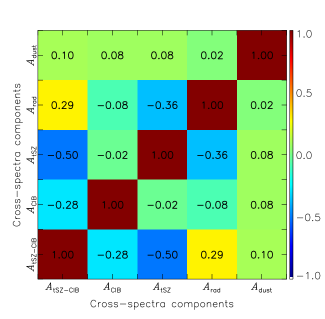
Figure 16: Correlation matrix for multi-frequency cross-spectra components from Eq. (5.2.2).

6 Conclusions and discussion

We have performed a comprehensive analysis of the infrared emission from galaxy clusters. We have proposed a model of the tSZ-CIB correlation derived from coherent modelling of both the tSZ and CIB at galaxy clusters. We have shown that the models of the tSZ and CIB power spectra reproduce fairly well the observed power spectra from the Planck data. Using this approach, we have been able to predict the expected tSZ-CIB cross-spectrum. Our predictions are consistent with previous work reported in the literature (Addison et al. 2012; Zahn et al. 2012).

We have demonstrated that the CIB scaling relation from Planck Collaboration XXX (2014) is able to reproduce the observed stacked SED of Planck confirmed clusters. We have also set constraints on the profile of the this emission and found that the infrared emission is more extended than the tSZ profile. We also find that the infrared profile is more extended than seen in previous work (see e.g., Xia et al. 2012) based on numerical simulation (Bullock et al. 2001). Fitting for the concentration of an NFW profile, the infrared emission shows $c_{500}=1.00^{+0.18}_{-0.15}$. This demonstrates that the infrared brightness of cluster-core galaxies is lower than that of outlying galaxies.

We have presented three distinct approaches for constraining the tSZ-CIB cross-correlation level: (i) using confirmed tSZ clusters; (ii) through cross-correlating a tSZ Compton parameter map with Planck frequency maps; and (iii) by directly cross-correlating Planck frequency maps. We have compared these analyses with the predictions from the model and derived consistent results. We obtain: (i) a detection of the tSZ-IR correlation at 6$\thinspace\sigma$; (ii) an amplitude $A_{\rm tSZ-CIB}=1.5\pm 0.5$; and (iii) an amplitude $A_{\rm tSZ-CIB}=1.2\pm 0.3$. At 143 GHz these values correspond to correlation coefficients at $\ell=3000$ of: (ii) $\rho=0.18\pm 0.07$; and (iii) $\rho=0.16\pm 0.04$. These results are consistent with previous analyses by the ACT collaboration, which set upper limits $\rho<0.2$ (Dunkley et al. 2013) and by the SPT collaboration, which found $\rho=0.11^{+0.06}_{-0.05}$ (George et al. 2014).

Our results, with a detection of the full tSZ-CIB cross-correlation amplitude at $4\thinspace\sigma$, provide the tightest constraint so far on the tSZ-CIB correlation factor. Such constraints on the tSZ-CIB cross-correlation are needed to perform an accurate measurement of the tSZ power spectrum. Beyond power spectrum analyses, the tSZ-CIB cross-correlation is also a major issue for relativistic tSZ studies, since CIB emission toward galaxy clusters mimics the relativistic tSZ correction and thus could produce significant bias if not accounted for properly. This $4\thinspace\sigma$ measurement of the amplitude of the tSZ-CIB correlation will also be important for estimates of the “kinetic” SZ power spectrum.