A hybrid recursive multilevel incomplete factorization preconditioner for solving general linear systems

Abstract

In this paper we introduce an algebraic recursive multilevel incomplete factorization preconditioner, based on a distributed Schur complement formulation, for solving general linear systems. The novelty of the proposed method is to combine factorization techniques of both implicit and explicit type, recursive combinatorial algorithms, multilevel mechanisms and overlapping strategies to maximize sparsity in the inverse factors and consequently reduce the factorization costs. Numerical experiments demonstrate the good potential of the proposed solver to precondition effectively general linear systems, also against other state-of-the-art iterative solvers of both implicit and explicit form.

Keywords: linear systems; iterative solvers; preconditioners; sparse approximate inverse methods; multilevel reordering algorithms.

1 Introduction

Krylov subspace methods may be considered the method of choice for solving large and sparse systems of linear equations arising from the discretization of (systems of) partial differential equations on modern parallel computers. This class of algorithms are iterative in nature. At every step $k$, they compute the approximate solution $x_{k}$ of a linear system $Ax=b$ from the Krylov subspace of dimension $k$

$$K_{k}(A,b)=span\large\{b,Ab,A^{2}b,\ldots,A^{k-1}b\},$$

according to different criteria for each given method. The computation requires matrix-vector products with the coefficient matrix $A$ plus vector operations, thus potentially reducing the cumbersome costs of sparse direct solvers on large problems, especially in terms of memory. All of the iterative Krylov methods converge rapidly if $A$ is somehow close to the identity. Therefore, it is common replacing the original system $Ax=b$ by

$$M^{-1}Ax=M^{-1}b,$$ (1)

or

$$AM^{-1}y=b,~{}~{}x=M^{-1}y,$$ (2)

for a nonsingular matrix $M\approx A$. Systems (1) and (2) are referred to as left and right preconditioned systems, respectively, and $M$ as the preconditioner matrix. In the case $M$ is factorized as the product of two sparse matrices, $M=M_{1}M_{2}$, like in the Hermitian and positive definite case, one might solve the modified linear system

$$M_{1}^{-1}AM_{2}^{-T}y=M_{1}^{-1}b,~{}~{}x=M_{2}^{-T}y.$$ (3)

If one may choose $M$ so that $M^{-1}A$, $AM^{-1}$ or $M_{1}^{-1}AM_{2}^{-T}$ approximate the identity, and linear systems with $M$ or with $M_{1}$ and $M_{2}$ as coefficient matrices are easy to invert, it is more efficient to apply a Krylov subspace method to the modified linear system.

Optimal analytic preconditioners based on low order discretizations, nearby equations that are simple to solve, or similar ideas have been proposed in the literature for specific problems. However, the problem-specific approach is generally sensitive to the characteristics of the underlying operator and to the details of the geometry. In this study, we pursue an algebraic approach where the preconditioner $M$ is computed only from the coefficient matrix $A$. Although not optimal for any specific problem, algebraic methods are universally applicable, they can be adapted to different operators and to changes in the geometry by tuning a few parameters, and are well suited for solving irregular problems defined on unstructured grids.

Roughly speaking, most of the existing techniques can be divided into either implicit or explicit form. A preconditioner of implicit form is defined by any nonsingular matrix $M\approx A$, and requires to solve an extra linear system with $M$ at each step of an iterative method. The most important example in this class is represented by the Incomplete $LU$ decomposition (ILU), where $M$ is implicitly defined as $M=\bar{L}\bar{U}$, $\bar{L}$ and $\bar{U}$ being triangular matrices that approximate the exact $L$ and $U$ factors of $A$ according to a prescribed dropping strategy adopted during the Gaussian elimination process. These methods are considered amongst the most reliable in a general setting. Well known theoretical results on the existence and the stability of the factorization can be proved for the class of $M$-matrices [mevd:77], and recent studies are involving more general matrices, both structured and unstructured. The quality of the factorization on difficult problems can be enhanced by using several techniques such as reordering, scaling, diagonal shifting, pivoting and condition estimators (see e.g. [duko:99a, ARMS, mmbw:00, BolS06, cabo:12]). As a result of this active development, in the last years successful results are reported with ILU-type preconditioners in many areas that were of exclusive domain of direct solution methods like in circuits simulation, power system networks, chemical engineering plants modelling, graphs and other problems not governed by PDEs, or in areas where direct methods have been traditionally preferred, like in structural analysis, semiconductor device modelling and computational fluid dynamics applications (see e.g. [saad:2005, boll:2003, Benzi02, Manguoglu2011, SaSoTo02]). One problem with ILU-techniques is the severe degradation of performance observed on vector, parallel and GPUs machines, mainly due to the sparse triangular solves [lisa:13]. In some cases, reordering techniques may help to introduce nontrivial parallelism. However, parallel orderings may sometimes degrade the convergence rate, while more fill-in diminishes the overall parallelism of the solver [dume:89].

Explicit preconditioning tries to mitigate such difficulties by approximating directly $A^{-1}$, as the product $M$ of sparse matrices, so that the preconditioning operation reduces to forming one (or more) sparse matrix-vector product, and consequently the application of the preconditioner may be easier to parallelize and numerically stable. Some methods can also perform the construction phase in parallel [huckle10efficient, cdgs:05, BFSAI, pash:14, pash:14a]; additionally, on certain indefinite problems with large nonsymmetric parts, the explicit approach can provide better results than ILU techniques (see e.g. [chsa:98, carp:07d, huckle10smoothing]). In practice, however, some questions need to be addressed. The computed matrix $M$ could be singular, and the construction cost is typically much higher than for ILU-type methods, especially for sequential runs. The main issue is the selection of the non-zero pattern of $M$. The idea is to keep $M$ reasonably sparse while trying to capture the ‘large’ entries of the inverse, which are expected to contribute the most to the quality of the preconditioner. On general problems it is difficult to determine the best structure for $M$ in advance, and the computational and storage costs required to achieve the same rate of convergence of preconditioners given in implicit form may be prohibitive in practice.

In this study, we present an algebraic multilevel solver for preconditioning general nonsymmetric linear systems which attempts to combine characteristics of both approaches. Assuming that the matrix $A$ admits the factorization $A=LU$, with $L$ a unit lower and $U$ an upper triangular matrix, our method approximates the inverse factors $L^{-1}$ and $U^{-1}$. Sparsity in the approximate inverse factors is maximized by employing recursive combinatorial algorithms. Robustness is enhanced by combining the factorization with recently developed overlapping strategies and by using efficient local solvers.

The paper is organized as follows. In Section 2 we describe the proposed multilevel preconditioner. In Section 3 we show how to combine our preconditioner with overlapping strategies, and in Section LABEL:sec:5 we assess its overall performance by showing several numerical experiments on realistic matrix problems, also against other state-of-the-art solvers. Finally, in Section LABEL:sec:6 we conclude the study with some remarks and perspectives for future work.

2 The AMES solver

Let

$$Ax=b$$ (4)

be a $n\times n$ general linear system with nonsingular, possibly indefinite and nonsymmetric matrix $A=\{a_{ij}\}\in\mathbb{R}^{n\times n}$, and vectors $x,b\in\mathbb{R}^{n}$. We assume that $A$ admits for a triangular decomposition

$$A=LU$$

and we precondition system (4) as

$$M_{L}AM_{U}y=M_{L}b$$

with $M_{L}\approx L^{-1}$ and $M_{U}\approx U^{-1}$, clearly preserving symmetry and/or positive definiteness of $A$. This approach of preconditioning linear systems has been extensively investigated in a series of papers by Kolotilina and Yeremin  [koye:93, koye:95, koyn:00, koyn:99], who prescribed the nonzero pattern of the inverse factors $M_{L}$ and $M_{U}$ of $A$ in advance equal to the pattern of the lower and upper triangular part of $A+A^{T}$, respectively, and determined the entries of $M_{L}$ and $M_{U}$ explicitly by solving linear equations involving the principal submatrices of $A$ (the ‘FSAI’ preconditioner). Chow suggested to use as pattern for the inverse factors the structure of the lower and upper triangular part of $(A+A^{T})^{p}$, where $p$ is a positive integer [chow:00a, chow:01, yuni:04]. The larger $p$, in general the higher the quality of the computed preconditioner, although the construction, storage and application costs tend to increase rapidly with $p$. Blocking and adaptive strategies have been recently studied to overcome these problems [BFSAI, gBFSAI, JANNA]. Benzi and Tuma proposed to compute the entries of matrices $M_{L}$ and $M_{U}$ by means of a (two-sided) Gram-Schmidt orthogonalization process with respect to the bilinear form associated with $A$, and to determine the best structure for the inverse factors dynamically, during the construction (the ‘AINV’ preconditioner). Sparsity is preserved in the process by discarding elements having magnitude smaller than a given positive threshold [bemt:96, betu:98b].

In this study we analyse multilevel mechanisms, recursive combinatorial algorithms and overlapping techniques, combined with efficient local solvers, to enhance robustness and reduce costs for the approximation of the inverse factors. We refer to the resulting preconditioner as AMES (Algebraic Multilevel Explicit Solver). It is easier to describe the AMES method by using graph notation, dividing the solution of system (4) in five distinct phases:

1. a scale phase, where the coefficient matrix $A$ is scaled by rows and columns so that the largest entry of the scaled matrix has magnitude smaller than one;

2. a preorder phase, where the structure of $A$ is used to compute a suitable ordering that maximizes sparsity in the approximate inverse factors;

3. an analysis phase, where the sparsity preserving ordering is analyzed and an efficient data structure is generated for the factorization;

4. a factorization phase, where the nonzero entries of the preconditioner are computed;

5. a solve phase, where all the data structures are accessed for solving the linear system.

Below we describe each phase separately.

2.1 Scale phase.

We initially scale system (4) by rows and columns as

$$D_{1}^{1/2}Ay=D_{1}^{1/2}b,~{}~{}y=D_{2}^{1/2}x,$$ (5)

where the ${n\times n}$ diagonal scaling matrices $D_{1}$ and $D_{2}$ have the form

$$D_{1}(i,j)=\left\{{\begin{array}[]{*{20}c}{\frac{1}{{\mathop{\max\left|{a_{ij}}\right|}\limits_{i}}}}&,\rm{~{}~{}if~{}i~{}=~{}j}\\ &\\ 0&,\rm{~{}~{}if~{}i~{}\neq~{}j}\\ \end{array}}\right.,~{}~{}~{}D_{2}(i,j)=\left\{{\begin{array}[]{*{20}c}{\frac{1}{{\mathop{\max\left|{a_{ij}}\right|}\limits_{j}}}}&,\rm{~{}~{}if~{}i~{}=~{}j}\\ &\\ 0&,\rm{~{}~{}if~{}i~{}\neq~{}j}\\ \end{array}}\right.~{}.$$

For simplicity, we still refer in this paper to the scaled system (5) as $Ax=b$.

2.2 Preorder phase.

We use standard notation of graph theory to describe this computational step. We denote by $\Omega(\tilde{A})$ the undirected graph associated with the matrix

$$\tilde{A}=\left\{\begin{array}[]{l}A,~{}~{}~{}~{}~{}~{}~{}~{}{\rm{~{}if~{}}}A{{\rm{~{}is~{}symmetric,}}}\\ A+A^{T},{\rm{~{}if~{}}}A{{\rm{~{}is~{}nonsymmetric.}}}\\ \end{array}\right.$$

First, $\Omega(\tilde{A})$ is partitioned into $p$ non-overlapping subgraphs $\Omega_{i}$ of roughly equal size by using the multilevel graph partitioning algorithms available in the Metis package [METIS]. For each partition $\Omega_{i}$ we distinguish two disjoint sets of nodes (or vertices): interior nodes that are connected only to nodes in the same partition, and interface nodes that straddle between two different partitions; the set of interior nodes of $\Omega_{i}$ form a so called separable or independent cluster. Upon renumbering the vertices of $\Omega$ one cluster after another, followed by the interface nodes as last, and permuting $A$ according to this new ordering, a block bordered linear system is obtained, with coefficient matrix of the form

$$\tilde{A}=P^{T}AP=\left({\begin{array}[]{*{20}c}B&F\\ E&C\\ \end{array}}\right)=\left({\begin{array}[]{*{20}c}{B_{1}}&{}\hfil&{}\hfil&{}\hfil&{F_{1}}\\ {}\hfil&{B_{2}}&{}\hfil&{}\hfil&{F_{2}}\\ {}\hfil&{}\hfil&\ddots&{}\hfil&\vdots\\ {}\hfil&{}\hfil&{}\hfil&{B_{p}}&{F_{p}}\\ {E_{1}}&{E_{2}}&\cdots&{E_{p}}&{C}\\ \end{array}}\right).$$ (6)

In (6), each diagonal block $B_{i}$ corresponds to the interior nodes of $\Omega_{i}$, and the blocks $E_{i}$ and $F_{i}$ correspond to the interface nodes of $\Omega_{i}$; the block $C$ is associated to the mutual interactions between the interface nodes. In our multilevel scheme we apply the same block downward arrow structure to the diagonal blocks $B_{i}$ of $\tilde{A}$; the procedure is repeated recursively until a maximum number of levels is reached, or until the blocks at the last level are sufficiently small to be easily factorized. As an example, in Figure 1(b) we show the structure of the sparse matrix rdb2048 from Tim Davis’ matrix collection [timdavis] after three reordering levels.

To reduce factorization costs, a similar permutation is applied to the Schur complement matrix $S=C-EB^{-1}F$ as follows

$$\tilde{S}=\left({\begin{array}[]{*{20}c}{B_{S1}}&{}\hfil&{}\hfil&{}\hfil&{F_{S1}}\\ {}\hfil&{B_{S2}}&{}\hfil&{}\hfil&{F_{S2}}\\ {}\hfil&{}\hfil&\ddots&{}\hfil&\vdots\\ {}\hfil&{}\hfil&{}\hfil&{B_{Sp}}&{F_{Sp}}\\ {E_{S1}}&{E_{S2}}&\cdots&{E_{Sp}}&{C_{S}}\\ \end{array}}\right).$$ (7)

2.3 Analysis phase.

In the analysis phase, a suitable data structure for storing the linear system is defined, allocated and initialized. We use a tree structure to store the block bordered form (6) of $\tilde{A}$. The root is the whole graph $\Omega$, and the leaves at each level are the independent clusters of each subgraph. Each node of the tree corresponds to one partition $\Omega_{i}$ of $\Omega(\tilde{A})$, or equivalently to one block $B_{i}$ of matrix $\tilde{A}$. The information stored at each node are the entries of the off-diagonal blocks $E$ and $F$ of $B_{i}^{\prime}s$ father, and those of the block $C$ of $B_{i}$ after its permutation, except at the last level of the tree where we store the entire block $B_{i}$. All these matrices are represented in the computer memory using a compressed sparse row storage format, except for blocks $F_{i}$ that are stored in compressed sparse column format. Blocks $E_{i}$ and $F_{i}$ can be very sparse; many of their rows and columns can be zero, and this leads to a significant saving of computation.

2.4 Factorization phase.

The approximate inverse factors $\tilde{L}^{-1}$ and $\tilde{U}^{-1}$ of $\tilde{A}$ write in the following form

$$\tilde{L}^{-1}\approx\left({\begin{array}[]{*{20}c}{U_{1}^{-1}}&{}\hfil&{}\hfil&{}\hfil&{W_{1}}\\ {}\hfil&{U_{2}^{-1}}&{}\hfil&{}\hfil&{W_{2}}\\ {}\hfil&{}\hfil&\ddots&{}\hfil&\vdots\\ {}\hfil&{}\hfil&{}\hfil&{U_{p}^{-1}}&{W_{p}}\\ {}\hfil&{}\hfil&{}\hfil&{}\hfil&{U_{S}^{-1}}\\ \end{array}}\right),~{}~{}\tilde{U}^{-1}\approx\left({\begin{array}[]{*{20}c}{L_{1}^{-1}}&{}\hfil&{}\hfil&{}\hfil&{}\hfil\\ {}\hfil&{L_{2}^{-1}}&{}\hfil&{}\hfil&{}\hfil\\ {}\hfil&{}\hfil&\ddots&{}\hfil&{}\hfil\\ {}\hfil&{}\hfil&{}\hfil&{L_{p}^{-1}}&{}\hfil\\ {G_{1}}&{G_{2}}&\cdots&{G_{p}}&{L_{S}^{-1}}\\ \end{array}}\right)$$ (8)

where

$$B_{i}=L_{i}U_{i},W_{i}=-U_{i}^{-1}L_{i}^{-1}F_{i}U_{S}^{-1},G_{i}=-L_{S}^{-1}E_{i}U_{i}^{-1}L_{i}^{-1}$$ (9)

and $L_{S},U_{S}$ are the triangular factors of the Schur complement matrix

$$S=C-\sum\limits_{i=1}^{p}{E_{i}B_{i}^{-1}F_{i}}.$$ (10)

Some fill-in may occur in $\tilde{L}^{-1}$ and $\tilde{U}^{-1}$ during the factorization, but only within the nonzero blocks. This two-level reordering scheme was used in the context of factorised approximate inverse methods for the parallelization of the AINV preconditioner in [bemt:07]. Differently from [bemt:07], we apply the arrow structure (6) recursively to the diagonal blocks and to the first level Schur complement as well, to gain additional sparsity. The multilevel factorization algorithm requires to invert only the last level blocks and the small Schur complements at each reordering level; the blocks $W_{i}$, $G_{i}$ do not need to be assembled explicitly, as they may be applied using Eqn (9). For the rdb2048 problem, in Figure 1(c) we display in red the actual extra storage required by the exact multilevel inverse factorization in addition to matrix $A$; these represent only $34\%$ of the total nonzeros of $A$. From the knowledge of the red entries, the blue ones can be retrieved from Eqn (9), using the off-diagonal blocks of $A$.

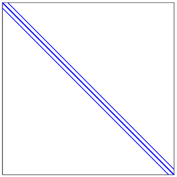
(a) The original structure of the rdb2048 matrix.

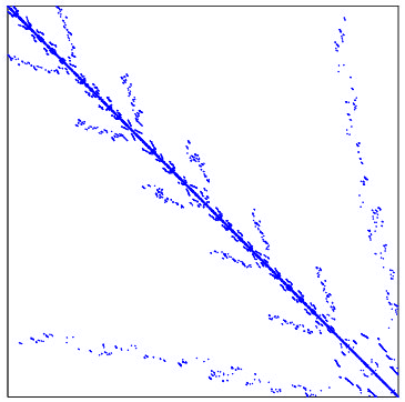
(b) The structure of rdb2048 after permutation.

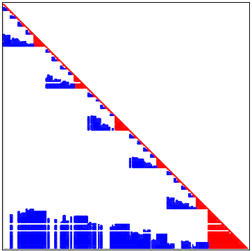
(c) The structure of the inverse factor. In red are displayed the entries actually stored.

Figure 1: Structure of the multilevel inverse-based factorization for the matrix rdb2048.

We also permute the large Schur complement at the first level into a block bordered structure, until we reach a maximal number of levels or a given minimal size. The last-level matrix is inverted inexactly. An inexact solver is also used to factorize the last-level blocks $B_{i}$ in (10).

2.5 Solve phase.

In the solve phase, the multilevel factorization is applied at every iteration step of a Krylov method for solving the linear system. Notice that the inverse factorization of $\tilde{A}$ may be written as

$$\left(PAP^{T}\right)^{-1}=\left({\begin{array}[]{*{20}c}{U^{-1}}&W\\ 0&{U_{S}^{-1}}\\ \end{array}}\right)\times\left({\begin{array}[]{*{20}c}{L^{-1}}&0\\ G&{L_{S}^{-1}}\\ \end{array}}\right)$$ (11)

where $W=-U^{-1}L^{-1}FU_{S}^{-1},~{}G=-L_{S}^{-1}EU^{-1}L^{-1}$, and $L_{S},~{}U_{S}$ are the inverse factors of the Schur complement matrix $S=C-EB^{-1}F$.

From Eqn. (11), we obtain the following expression for the exact inverse

$$\left({\begin{array}[]{*{20}c}{B^{-1}+B^{-1}FS^{-1}EB^{-1}}&{-B^{-1}FS^{-1}}\\ {-S^{-1}EB^{-1}}&{S^{-1}}\\ \end{array}}\right).$$ (12)

We can derive preconditioners from Eqn. (12) by computing approximate solvers $\tilde{B}^{-1}$ for $B$ and $\tilde{S}^{-1}$ for $S$. Hence the preconditioner matrix $M$ will have the form

$$M=\left({\begin{array}[]{*{20}c}{\tilde{B}^{-1}+\tilde{B}^{-1}F\tilde{S}^{-1}E\tilde{B}^{-1}}&{-\tilde{B}^{-1}F\tilde{S}^{-1}}\\ {-\tilde{S}^{-1}E\tilde{B}^{-1}}&{\tilde{S}^{-1}}\\ \end{array}}\right).$$

and the preconditioning operation $\left[{\begin{array}[]{*{20}c}{y_{1}}\\ {y_{2}}\\ \end{array}}\right]=M\left[{\begin{array}[]{*{20}c}{x_{1}}\\ {x_{2}}\\ \end{array}}\right]$ writes as Algorithm 1. Notice that Algorithm 1 is called recursively at lines 1-3, as $\tilde{B}$ and $\tilde{S}$ also have a block bordered structure upon permutation.

Algorithm 1 The preconditioning operation in the AMES solver.

1:  $p_{1}=\tilde{B}^{-1}x_{1}$

2:  $[p_{2},p_{3}]=\tilde{S}^{-1}[E\cdot p_{1},x_{2}]$

3:  $[p_{4},p_{5}]=\tilde{B}^{-1}[F\cdot p_{2},F\cdot p_{3}]$

4:  $y_{1}=p_{1}+p_{4}-p_{5}$

5:  $y_{2}=p_{3}-p_{2}$

3 Combining the AMES solver with overlapping

In [overlapping], Grigori, Nataf and Qu have introduced an overlapping technique to enhance the robustness of multilevel incomplete LU factorization preconditioning computed from matrices reordered in arrow form, e.g. using the nested dissection method by George [geli:81]. The multilevel mechanism incorporated in the AMES preconditioner described in the previous section is based on a nested dissection-like ordering, and thus it can easily accomodate for overlapping. We have tested this idea in our numerical experiments, and in this section we shortly describe the procedure adopted. The results of our experiments are reported in Section LABEL:sec:5.

3.1 Background

Let $\Omega=(V(\Omega),E(\Omega))$ be the graph of $A$, $V(\Omega)$ denoting the set of vertices and $E(\Omega)$ the set of edges in $\Omega$. If the graph is directed, we denote an edge of $E$ issuing from vertex $u$ to vertex $v$ as $(u,v)$; $u$ is called a predecessor of $v$, and $v$ a successor of $u$. If the graph is undirected, we denote the edges of $E$ by non-ordered pairs $\{u,v\}$; $u$ is called a neighbour of $v$. As in the previous section, we assume that $\Omega$ is partitioned into $p$ independent non-overlapping subgraphs $\Omega_{1}$, $\ldots$, $\Omega_{p}$, and we call $S$ the set of separator nodes, straddling between two different partitions. Goal of overlapping is to extend each independent set of $\Omega$ by including its direct neighbours, similarly to the overlapping idea used in other domain decomposition methods, for example in the restricted additive Schwarz method [quva:99, SAAD-BOOK].

Following [overlapping], we denote by $V(\Omega_{i,ext})$ the separator nodes that are successors of $\Omega_{i}$,

$$V(\Omega_{i,ext})=\{v\in V(S)|\exists u\in V(\Omega_{i}),(u,v)\in E(\Omega)\}\subset V(S),$$ (13)

and by $V(\Omega_{ext})$ the complete set of successor nodes of all the subdomains

$$V(\Omega_{ext})=\bigcup_{i=1:p}V(\Omega_{i,ext}).$$ (14)

Then $\Omega_{i}$ is extended to the set $\hat{\Omega}_{i}$ as

$$V(\hat{\Omega}_{i})=V(\Omega_{i})\cup V(\Omega_{i,ext}),~{}i=1,\ldots,p,$$ (15)

and the separator $S$ is extended to $\hat{S}$ by adding the successors of nodes in $V(\Omega_{ext})$, that is

$$V(\hat{S})=V(S)\cup\{v\in V(\Omega_{i}),i=1,\ldots,p~{}|~{}\exists u\in V(\Omega_{ext}),(u,v)\in E(\Omega)\}.$$ (16)

Using this notation, the overlapped graph of $A$, $\tilde{\Omega}=(V(\tilde{\Omega}),E(\tilde{\Omega}))$, is introduced as follows. First define the overlapped subgraph $\tilde{\Omega}_{i}$ and the overlapped separator $\tilde{S}$ as, respectively,

$$V(\tilde{\Omega}_{i})=\{(x,i):x\in\hat{\Omega}_{i}\},$$

$$V(\tilde{S})=\{(x,s):x\in\hat{S}\}.$$

For simplicity we refer to $(x,i)$ as $x_{i}$. Then the vertex set $V(\tilde{\Omega})$ of the overlapped graph $\tilde{\Omega}$ is formed by the disjoint union of the $V(\hat{\Omega_{i}})$’s and of $V(\hat{S})$ as

$$V(\tilde{\Omega})=\left(\bigcup_{i\in 1:p}V(\hat{\Omega}_{i})\right)\cup V(\hat{S}).$$ (17)

Recall that, given the union $B$ of a family of sets indexed by the index set $I$,

$$B=\bigcup_{i\in I}A_{i}=\bigcup_{i\in I}\{x:x\in A_{i}\},$$

their disjoint union $C$ is defined as the set

$$C=\bigcup_{i\in I}\{(x,i):x\in A_{i}\}.$$

At this stage, it is useful to introduce the two projection operators $\Pi_{1}$ and $\Pi_{2}$ such that

$$\Pi_{1}:(x,i)\mapsto x$$

and

$$\Pi_{2}:(x,i)\mapsto i.$$

With this notation, the set of edges of the overlapped graph $\tilde{\Omega}$ is defined according to their projection onto the original graph as follows

$$E(\tilde{\Omega}_{i})=\{(u_{i},v_{i})|u_{i}\in V(\tilde{\Omega}_{i}),v_{i}\in V(\tilde{\Omega}_{i}),(\Pi_{1}(u_{i}),\Pi_{1}(v_{i}))\in E(\Omega)\},$$ (18)

$$E(\tilde{S})=\{(u_{s},v_{s})|u_{s}\in V(\tilde{S}),v_{s}\in V(\tilde{S}),(\Pi_{1}(u_{s}),\Pi_{1}(v_{s}))\in E(\Omega)\},$$ (19)

$$E(\tilde{\Omega}_{i},\tilde{S})=\{(u_{i},v_{s})|u_{i}\in V(\tilde{\Omega}_{i}),v_{s}\in V(\tilde{S}),(\Pi_{1}(u_{i}),\Pi_{1}(v_{s}))\in E(\Omega),$$

$$\nexists v_{i}\in V(\tilde{\Omega}_{i}),(u_{i},v_{i})\in E(\tilde{\Omega}_{i})\},$$ (20)

$$E(\tilde{S},\tilde{\Omega}_{i})=\{(u_{s},v_{i})|u_{s}\in V(\tilde{S}),v_{i}\in V(\tilde{\Omega}_{i}),(\Pi_{1}(u_{s}),\Pi_{1}(v_{i}))\in E(\Omega),$$

$$\nexists v_{s}\in V(\tilde{S}),(u_{s},v_{s})\in E(\tilde{S})\}.$$ (21)

The following property, established in [overlapping], ensures an equivalence between the equations of the overlapped system and those of the original system.

Property 1

Let $\Omega$ be the associated directed graph of a given system of linear equations and $u$ be a vertex of $V(\Omega)$. Let $\tilde{\Omega}$ be the overlapped graph, and let $u_{i}$ be a vertex of $V(\tilde{\Omega})$ such that $\Pi_{1}(u_{i})=u\in V(\Omega)$. For each edge $(u,v)\in E(\Omega)$, there is a unique $v_{j}\in V(\tilde{\Omega})$ such that we have both $\Pi_{1}(v_{j})=v$ and $(u_{i},v_{j})\in E(\tilde{\Omega})$.

This property shows that there exists a bijection between the nonzeros of the equation corresponding to vertex $u$ in the original system and the nonzeros of the equation corresponding to its dual $u_{i}$, where $\Pi_{1}(u_{i})=u$. From a matrix viewpoint, to each nonzero entry $\tilde{a}_{u_{i},v_{i}}$ in the overlapped matrix there is a unique nonzero entry $a_{u,v}$ in the original matrix, where $\Pi_{1}(u_{i})=u$ and $\Pi_{1}(v_{i})=v$. Therefore there is a one-to-one correspondence between equations in the original system and those in the overlapped system. By solving the overlapped system, we can automatically obtain the solution of the original system.

3.2 Example

We display a simple example from [overlapping] to describe shortly how the overlapping procedure works in practice. We consider a $5\times 5$ matrix having the structure shown in Figure LABEL:fig:smalloverlapping(a). The graph consists of two independent subgraphs $\Omega_{1}=\{1,2\}$, $\Omega_{2}=\{3\}$ and one separator $S=\{4,5\}$. We just pick the first subgraph and the separator set to explain. Separator nodes that are successors of $\Omega_{1}$ are the set

$$V(\Omega_{1,ext})=\{4,5\}$$

and we have

$$V(\hat{\Omega}_{1})=V(\Omega)_{1}\cup V(\Omega_{1,ext})=\{1,2,4,5\},$$

so that

$$V(\tilde{\Omega}_{1})=\{1_{1},2_{1},4_{1},5_{1}\}.$$

Analogously,

$$V(\Omega_{2,ext})=\{4,5\}$$

and

$$V(\Omega_{ext})=\Omega_{1,ext}\cup\Omega_{2,ext}=\{4,5\}.$$

Next, we compute the overlapped separator set $\tilde{S}$. The vertices of $V(\Omega_{1})$ and $V(\Omega_{2})$ directed by $V(\Omega_{ext})$ are $\{1,3\}$, so

$$V(\hat{S})=V(S)\cup\{1,3\}=\{4,5,1,3\}$$

and

$$V(\tilde{S})=\{4_{s},5_{s},1_{s},3_{s}\}.$$

According to Eqns. (18)-(21), the edges of the overlapped subdomain $E(\tilde{\Omega}_{1})$ are defined based on their projection onto the original graph. The first diagonal block of the overlapped matrix is formed by picking the $V(\hat{\Omega}_{1})=\{1,2,4,5\}$ rows and columns of the original matrix

$$\bordermatrix{&1&2&4&5\cr 1&\diamond&\diamond&\diamond&\diamond\cr 2&\diamond&\diamond&\ &\ \cr 4&\diamond&\ &\diamond&\ \cr 5&\diamond&\ &\ &\diamond\cr}.$$

Similarly for the other two diagonal blocks, and this is shown in Figure LABEL:fig:smalloverlapping(b).

From Eqn. (20), we can construct the edges from $\tilde{\Omega}_{1}$ to $\tilde{S}$. These are the nonzero entries of the overlapped interface block $\tilde{F}_{1}$, adopting the same notation as in (6). We pick the $V(\hat{\Omega}_{1})=\{1,2,4,5\}$ rows and $V(\hat{S})=\{4,5,1,3\}$ columns of the original matrix, and we set the columns corresponding to the common vertexes of $\hat{\Omega}_{1}$ and $\hat{S}$ to zeros. In our example this results in zeroing out the columns of $\hat{F}_{1}$ indexed by $\hat{\Omega}_{1}\cup\hat{S}=\{4,5,1\}$, giving

$$\begin{array}{ccccc}& 4& 5& 1& 3\\ 1& \times & \times & \diamond & \\ 2& & & \diamond & \\ 4& \star & & \times & \times \\ 5& & \times & \times & \times \end{array}$$