Semidefinite programming relaxations for linear semi-infinite polynomial programming

Abstract.

This paper studies a class of so-called linear semi-infinite polynomial programming (LSIPP) problems. It is a subclass of linear semi-infinite programming problems whose constraint functions are polynomials in parameters and index sets are basic semialgebraic sets. We present a hierarchy of semidefinite programming (SDP) relaxations for LSIPP problems. Convergence rate analysis of the SDP relaxations is established based on some existing results. We show how to verify the compactness of feasible sets of LSIPP problems. In the end, we extend the SDP relaxation method to more general semi-infinite programming problems.

Key words   linear semi-infinite programming, semidefinite programming relaxations, sum of squares, polynomial optimization

AMS subject classification   65K05, 90C22

1. introduction

We consider the following linear semi-infinite polynomial programming (LSIPP) problem

(1.1) $$(P)\qquad\left\{\begin{aligned} p^{*}:=\inf_{x\in{\mathbb{R}}^{m}}&\ c^{T}x\\ \text{s.t.}&\ a(y)^{T}x+b(y)\geq 0,\ \ \forall y\in S\subseteq{\mathbb{R}}^{n},\end{aligned}\right.$$

where $c\in{\mathbb{R}}^{m}$, $b(Y)\in{\mathbb{R}}[Y]:={\mathbb{R}}[Y_{1},\ldots,Y_{n}]$ the polynomial ring in $Y$ over the real field, $a(Y)=(a_{1}(Y),\ldots,a_{m}(Y))^{T}\in{\mathbb{R}}[Y]^{m}$, and the index set $S$ is a basic semialgebraic set defined by

(1.2) $$S:=\{y\in{\mathbb{R}}^{n}\mid g_{1}(y)\geq 0,\ldots,g_{s}(y)\geq 0\},$$

where $g_{j}(Y)\in{\mathbb{R}}[Y]$, $j=1,\dots,s$. Lowercase letters (e.g. $x,y,w$) are hereinafter used for denoting points in a space while uppercase letters (e.g. $X,Y,W$) for the corresponding variables. In this paper, we assume that $(\ref{eq::lsipp})$ is feasible and bounded from below, i.e., $-\infty<p^{*}<\infty$. Note that the problem $(\ref{eq::lsipp})$ is NP-hard. Indeed, it is obvious that the problem of minimizing a polynomial $f(Y)\in{\mathbb{R}}[Y]$ over $S$ can be regarded as a special LSIPP problem (see Example 3.22). As is well known, the polynomial optimization problem is NP-hard even when $n>1$, $f(Y)$ is a nonconvex quadratic polynomial and $g_{j}(Y)$’s are linear [36]. Hence, a general LSIPP problem cannot be expected to be solved in polynomial time unless P=NP.

LSIPP can be seen as a special branch of linear semi-infinite programming (LSIP), or more general, of semi-infinite programming (SIP), in which the involved functions are not necessarily polynomials. Numerically, SIP problems can be solved by different approaches including, for instance, discretization methods, local reduction methods, exchange methods, simplex-like methods and so on. See the surveys [10, 11, 28] and the references therein for details. One of main difficulties in numerical treatment of general SIP problems is that the feasibility test of a point $\bar{u}\in{\mathbb{R}}^{m}$ is equivalent to globally solving the problem of minimizing the constraint function with fixed $\bar{u}$ over the index set, which is called the lower level subproblem. Typically, when solving SIP problems by existing methods in the literature, the main difficulty lies in solving the nonlinear lower level subproblems at each iteration.

LSIPP, as a special subclass of SIP, has many applications like minimax problems, functional approximation problems. However, to the best of our knowledge, few of the numerical methods mentioned above are specially designed by exploiting features of polynomial optimization problems. Parpas and Rustem [37] proposed a discretization-like method to solve minimax polynomial optimization problems, which can be reformulated as semi-infinite polynomial programming (SIPP) problems. Using polynomial approximation and an appropriate hierarchy of semidefinite programming (SDP) relaxations, Lasserre presented an algorithm to solve the generalized SIPP problems in [24]. Based on an exchange scheme, an SDP relaxation method for solving SIPP problems was proposed in [44]. By using representations of nonnegative polynomials in the univariate case, an SDP method was given in [46] for LSIPP problems $(\ref{eq::lsipp})$ with $S$ being closed intervals.

In this paper, we propose a hierarchy of SDP relaxations for LSIPP (1.1). The dual problem of LSIPP is a special case of the generalized moment problems (Section 2.2), which has been well investigated, see [2, 3, 4, 19, 20, 23, 34] and the references therein. Lasserre [23] proposed an SDP relaxation method for generalized moment problems based on Putinar’s Positivstellensatz [39]. Although the SDP relaxations presented in this paper can be seen as the dual of Lasserre’s relaxations for GPM, they are of their independent interest because of the following desirable features they enjoy. First, some (approximate) minimizers of (1.1) can be extracted by these SDP relaxations, which is very useful in some applications, like functional approximation problems (Example 3.8); Second, convergence rate of these SDP relaxations can be estimated (Section 3.2) by using the complexity analysis of Putinar’s Positivstellensatz in [35]; Third, these SDP relaxations can be easily extended to more general semi-infinite programming problems (Section 4), like problems of the form (1.1) with semialgebraic functions, or with s.o.s-convex objectives. As the feasible set of (1.1) is assumed to be compact in the convergence rate estimation, we also show that the compactness can be verified by computing a positive lower bound of the infima of several LSIPP problems. It can be done by the proposed SDP relaxations if the finite convergence happens (in particular, if $S$ is a closed and bounded interval (Section 3.3)).

This paper is organized as follows. We introduce some notation and preliminaries in Section 2. SDP relaxations of LSIPP problems and the convergence rate analysis is given in Section 3, where we also discuss how to verify the compactness of feasible sets of LSIPP problems. In Section 4, we extend the SDP relaxation method to more general semi-infinite programming problems. Some conclusions are made in Section 5.

2. Notation and Preliminaries

Here is some notation used in this paper. The symbol $\mathbb{N}$ (resp., $\mathbb{R}$) denotes the set of nonnegative integers (resp., real numbers). For any $t\in\mathbb{R}$, $\lceil t\rceil$ denotes the smallest integer that is not smaller than $t$. For $y=(y_{1},\ldots,y_{n})\in\mathbb{R}^{n}$, $\|y\|_{2}$ denotes the standard Euclidean norm of $y$. For $\alpha=(\alpha_{1},\ldots,\alpha_{n})\in\mathbb{N}^{n}$, $\|\alpha\|_{1}:=\alpha_{1}+\cdots+\alpha_{n}$. For $k\in\mathbb{N}$, denote $\mathbb{N}^{n}_{k}=\{\alpha\in\mathbb{N}^{n}\mid\|\alpha\|_{1}\leq k\}$. For $y\in\mathbb{R}^{n}$ and $\alpha\in\mathbb{N}^{n}$, $y^{\alpha}$ denotes $y_{1}^{\alpha_{1}}\cdots y_{n}^{\alpha_{n}}$. $\mathbb{R}[Y]=\mathbb{R}[Y_{1},\cdots,Y_{n}]$ denotes the ring of polynomials in $(Y_{1},\cdots,Y_{n})$ with real coefficients. For $k\in\mathbb{N}$, denote by ${\mathbb{R}}[Y]_{k}$ the set of polynomials in ${\mathbb{R}}[Y]$ of total degree up to $k$. For a symmetric matrix $Z$, $Z\succeq 0(\succ 0)$ means that $Z$ is positive semidefinite (definite). For $m\in\mathbb{N}$, ${\mathbb{R}}^{m\times m}$ denotes the set of $m\times m$ real matrices and $\mathbb{S}_{+}^{m}\subset{\mathbb{R}}^{m\times m}$ denotes its subset of positive semidefinite matrices. For two symmetric matrices $A,B$ of the same size, $\langle A,B\rangle$ denotes the inner product of $A$ and $B$.

2.1. Sums of squares and moments

We recall some background about sums of squares (s.o.s) of polynomials and the dual theory of moment matrices. For any $f(Y)\in{\mathbb{R}}[Y]_{k}$, let $\bf{f}$ denote its column vector of coefficients in the canonical monomial basis of ${\mathbb{R}}[Y]_{k}$. A polynomial $f(Y)\in{\mathbb{R}}[Y]$ is said to be a sum of squares of polynomials if it can be written as $f(Y)=\sum_{i=1}^{t}f_{i}(Y)^{2}$ for some $f_{1}(Y),\ldots,f_{t}(Y)\in{\mathbb{R}}[Y]$. The symbol $\Sigma^{2}[Y]$ denotes the set of polynomials that are s.o.s.

Let $G:=\{g_{1},\ldots,g_{s}\}$ be the set of polynomials that define the semialgebraic set $S$ $(\ref{eq::S})$. We denote by

$$\mathcal{Q}(G):=\left\{\sum_{j=0}^{s}\sigma_{j}g_{j}\ \Big{|}\ g_{0}=1,\ \sigma_{j}\in\Sigma^{2}[Y],j=0,1,\ldots,s\right\}$$

the quadratic module generated by $G$ and denote by

$$\mathcal{Q}_{k}(G):=\left\{\sum_{j=0}^{s}\sigma_{j}g_{j}\ \Big{|}\ g_{0}=1,\ \sigma_{j}\in\Sigma^{2}[Y],\,\deg(\sigma_{j}g_{j})\leq 2k,j=0,1,\ldots,s\right\}$$

its $k$-th quadratic module. It is clear that if $f\in\mathcal{Q}(G)$, then $f(y)\geq 0$ for any $y\in S$. However, the converse is not necessarily true, see Example 3.20. Note that checking whether $f\in\mathcal{Q}_{k}(G)$ for a fixed $k\in\mathbb{N}$ is an SDP feasibility problem [21].

For $k\in\mathbb{N}$, denote $s(k):={n+k\choose n}$. Consider a finite sequence of real numbers $z:=(z_{\alpha})_{\alpha\in\mathbb{N}^{n}_{2k}}\in{\mathbb{R}}^{s(2k)}$ whose elements are indexed by $n$-tuples $\alpha\in\mathbb{N}^{n}_{2k}$. $z$ is called a truncated moment sequence up to order $2k$ if there exists a Borel measure $\mu$ on ${\mathbb{R}}^{n}$ such that

$$z_{\alpha}=\int Y^{\alpha}\mathrm{d}\mu(y),\ \forall\alpha\in\mathbb{N}^{n}_{2k}.$$

In this case, we say that $z$ has a representing measure $\mu$. The associated $k$-th moment matrix is the matrix $M_{k}(z)$ indexed by $\mathbb{N}^{n}_{k}$, with $(\alpha,\beta)$-th entry $z_{\alpha+\beta}$ for $\alpha,\beta\in\mathbb{N}^{n}_{k}$. Given a polynomial $f(Y)=\sum_{\alpha}f_{\alpha}Y^{\alpha}$, for $k\geq d_{f}:=\lceil\deg(f)/2\rceil$, the $(k-d_{f})$-th localizing moment matrix $M_{k-d_{f}}(fz)$ is defined as the moment matrix of the shifted vector $((fz)_{\alpha})_{\alpha\in\mathbb{N}^{n}_{2(k-d_{f})}}$ with $(fz)_{\alpha}=\sum_{\beta}f_{\beta}z_{\alpha+\beta}$. ${\mathscr{M}_{2k}}$ denotes the space of all sequences $z=(z_{\alpha})_{\alpha\in\mathbb{N}^{n}_{2k}}\in{\mathbb{R}}^{s(2k)}$ with order at most $2k$. For any $z\in\mathscr{M}_{2k}$, the corresponding Riesz functional $\mathscr{L}_{z}$ on ${\mathbb{R}}[Y]_{2k}$ is defined by

$$\mathscr{L}_{z}\left(\sum_{\alpha}q_{\alpha}Y_{1}^{\alpha_{1}}\cdots Y_{n}^{\alpha_{n}}\right):=\sum_{\alpha}q_{\alpha}z_{\alpha},\quad\forall q(Y)\in{\mathbb{R}}[Y]_{2k}.$$

From the definition of the localizing moment matrix $M_{k-d_{f}}(fz)$, it is easy to check that

(2.1) $$\mathbf{q}^{T}M_{k-d_{f}}(fz)\mathbf{q}=\mathscr{L}_{z}(f(Y)q(Y)^{2}),\quad\forall q(Y)\in{\mathbb{R}}[Y]_{k-d_{f}}.$$

Let $d_{j}:=\lceil\deg(g_{j})/2\rceil$ for each $j=1,\ldots,s$. For any $v\in S$, let $\zeta_{2k,v}:=[v^{\alpha}]_{\alpha\in\mathbb{N}^{n}_{2k}}$ be the Zeta vector of $v$ up to degree $2k$, i.e.,

$$\zeta_{2k,v}=[1\quad v_{1}\quad\cdots\quad v_{n}\quad v_{1}^{2}\quad v_{1}v_{2}\quad\cdots\quad v_{n}^{2k}].$$

Then, $M_{k}(\zeta_{2k,v})\succeq 0$ and $M_{k-d_{j}}(g_{j}\zeta_{2k,v})\succeq 0$ for $j=1,\ldots,s$. In fact, let $g_{0}=1$, then for each $j=0,1,\ldots,s$,

$$\mathbf{q}^{T}M_{k-d_{j}}(g_{j}\zeta_{2k,v})\mathbf{q} =\mathscr{L}_{\zeta_{2k,v}}(g_{j}(Y)q(Y)^{2})=g_{j}(v)q(v)^{2}\geq 0,\ \forall q(Y)\in{\mathbb{R}}[Y]_{k-d_{j}}.$$

Definition 2.1.

We say that ${\cal Q}(G)$ is Archimedean if there exists $\psi\in{\cal Q}(G)$ such that the inequality $\psi(y)\geq 0$ defines a compact set in ${\mathbb{R}}^{n}$.

Note that the Archimedean property implies that $S$ is compact but the converse is not necessarily true. However, for any compact set $S$ we can always force the associated quadratic module to be Archimedean by adding a redundant constraint $M-\|y\|^{2}_{2}\geq 0$ in the description of $S$ for sufficiently large $M$.

Theorem 2.2.

[39, Putinar’s Positivstellensatz] Suppose that $\mathcal{Q}(G)$ is Archimedean.

1. If a polynomial $f\in{\mathbb{R}}[Y]$ is positive on $S$, then $f\in\mathcal{Q}_{k}(G)$ for some $k\in\mathbb{N}$;

2. If $M_{k}(z)\succeq 0$ and $M_{k}(g_{j}z)\succeq 0$ for all $j=1,\ldots,s$, and all $k=0,1,\ldots$, then $z=(z_{\alpha})_{\alpha\in\mathbb{N}^{n}}\in{\mathbb{R}}^{\mathbb{N}^{n}}$ has a representing measure $\mu$ supported by $S$.

2.2. Dual problems and GPM

The Lagrangian dual problem [17, 28, 41] of $(\ref{eq::lsipp})$ is

(2.2) $$\left\{\begin{aligned} d^{*}:=\sup_{\mu\in M^{+}(S)}&\ -\int_{S}b(y)\mathrm{d}\mu(y)\\ \text{s.t.}&\ \ \int_{S}a_{i}(y)\mathrm{d}\mu(y)=c_{i},\ i=1,\ldots,m,\end{aligned}\right.$$

where $M^{+}(S)$ is the space of all nonnegative bounded regular Borel measure supported by $S$. The dual problem (2.2) is in fact a special case of the so-called generalized problems of moments (GPM), which is to maximize a linear function over a linear section of the moment cone. We refer the interested readers to [2, 3, 20] and the references therein for various methodologies and applications of GPM problems. For numerical treatment of GPM problems, see [4, 19] for some geometric approaches and [23, 34] for SDP relaxation methods for GPM problems with polynomial data.

Now we introduce the main idea of the SDP relaxation method for (2.2) proposed by Lasserre in [23]. Assume that $S$ is compact, by Putinar’s Positivstellensatz (part $(ii)$ of Theorem 2.2), a sequence $z=(z_{\alpha})_{\alpha\in\mathbb{N}^{n}}\in{\mathbb{R}}^{\mathbb{N}^{n}}$ has a representing measure $\mu$ supported by $S$ if

$$M_{k}(z)\succeq 0,\quad M_{k}(g_{j}z)\succeq 0,\ j=1,\ldots,s,\ k=0,1,\ldots.$$

Define

(2.3) $$d_{j}:=\lceil\deg(g_{j})/2\rceil,\ d_{S}:=\max\{1,d_{1},\ldots,d_{s}\},$$

$$d_{P}:=\max\{d_{S},\lceil\deg(a_{1})/2\rceil,\cdots,\lceil\deg(a_{m})/2\rceil,\lceil\deg(b)/2\rceil\}.$$

Let $k\geq d_{P}$ and $z=(z_{\alpha})_{\alpha\in\mathbb{N}^{n}_{2k}}\in{\mathbb{R}}^{s(2k)}$, the $k$-th semidefinite relaxation of $(\ref{eq::Mdual})$ is

(2.4) $$\left\{\begin{aligned} p^{\mbox{\tiny mom}}_{k}:=\sup_{z\in{\mathbb{R}}^{s(2k)}}&\ -\sum_{\alpha\in\mathbb{N}^{n}_{2k}}b_{\alpha}z_{\alpha}\\ \text{s.t.}&\ \sum_{\alpha\in\mathbb{N}^{n}_{2k}}a_{i,\alpha}z_{\alpha}=c_{i},\ \ i=1,\ldots,m,\\ &\ M_{k}(z)\succeq 0,\ M_{k-d_{j}}(g_{j}z)\succeq 0,\ j=1,\ldots,s.\end{aligned}\right.$$

Under certain assumptions, Lasserre proved [23] that $p^{\mbox{\tiny mom}}_{k}$ decreasingly converges to $p^{*}$. The SDP relaxations $(\ref{eq::dsdplsipp})$ can be easily implemented and solved by the software GloptiPoly [16] developed by Henrion, Lasserre and Löfberg.

Condition 2.3.

An optimizer $z^{*}$ of the $k$-th SDP relaxation $(\ref{eq::dsdplsipp})$ satisfies the flat extension condition when

$$\mbox{rank}M_{k-d_{S}}(z^{*})=\mbox{rank}M_{k}(z^{*}).$$

Based on [7, Theorem 1.1], Lasserre [23, Theorem 2] showed that the finite convergence of (2.4) happens at order $k$ if the flat extension condition holds.

3. SDP relaxations of LSIPP

In this section, we present a hierarchy of SDP relaxations for LSIPP problems. These SDP relaxations can be seen as the dual of Lasserre’s relaxations for GPM and enjoy several desirable features. For example, (approximate) mininizers can be extracted and the convergence rate can be estimated by using some existing results. We shall also see in Section 4 that these SDP relaxations can be easily extended to more general semi-infinite programming problems.

3.1. SDP relaxations of LSIPP problems

We assume that $S$ in $(\ref{eq::lsipp})$ is compact. For a given feasible point $x\in{\mathbb{R}}^{m}$ of the LSIPP problem $(\ref{eq::lsipp})$, the constraint requires that the polynomial $a(Y)^{T}x+b(Y)\in{\mathbb{R}}[Y]$ is nonnegative on $S$. Since every polynomial in the quadratic module $\mathcal{Q}(G)$ of $S$ generated by $G$ is nonnegative on $S$, we can relax the problem $(\ref{eq::lsipp})$ as follows

(3.1) $$p^{\mbox{\tiny sos}}:=\inf_{x\in{\mathbb{R}}^{m}}\ \ c^{T}x\quad\text{s.t.}\ a(Y)^{T}x+b(Y)\in\mathcal{Q}(G).$$

Clearly, any feasible point of $(\ref{eq::qmrelax})$ is also feasible for $(\ref{eq::lsipp})$. Hence, we have $p^{\mbox{\tiny sos}}\geq p^{*}$.

Definition 3.1.

We say that the Slater condition holds for the problem $(\ref{eq::lsipp})$ if there exists $\bar{x}\in{\mathbb{R}}^{m}$ such that $a(y)^{T}\bar{x}+b(y)>0$ for all $y\in S$.

Theorem 3.2.

If $\mathcal{Q}(G)$ is Archimedean and the Slater condition holds for the LSIPP problem $(\ref{eq::lsipp})$, then $p^{\mbox{\tiny sos}}=p^{*}$.

Proof.

Fix an $\varepsilon>0$ and a feasible $\bar{x}\in{\mathbb{R}}^{m}$ of (1.1) such that $a(y)^{T}\bar{x}+b(y)>0$ for all $y\in S$. We next show that $p^{\mbox{\tiny sos}}-p^{*}<\varepsilon$. By Putinar’s Positivstellensatz, $\bar{x}$ is a feasible point of (3.1) and thus we can assume that $c\neq 0$ without loss of generality. If $c^{T}\bar{x}-p^{*}<\varepsilon$, then $p^{\mbox{\tiny sos}}-p^{*}\leq c^{T}\bar{x}-p^{*}<\varepsilon$ and we are done. Hence, we assume that $c^{T}\bar{x}-p^{*}\geq\varepsilon$ in the following. Then we can fix another feasible point $x^{\prime}\in{\mathbb{R}}^{m}$ of (1.1) such that $c^{T}\bar{x}>c^{T}x^{\prime}$ and $c^{T}x^{\prime}-p^{*}<\varepsilon/2$. Let

(3.2) $$\delta:=\frac{\varepsilon}{2c^{T}(\bar{x}-x^{\prime})}>0\quad\text{and}\quad\hat{x}:=(1-\delta)x^{\prime}+\delta\bar{x}.$$

Then we have $0<\delta<1$ and hence

(3.3) $$a(y)^{T}\hat{x}+b(y)=(1-\delta)[a(y)^{T}x^{\prime}+b(y)]+\delta[a(y)^{T}\bar{x}+b(y)]>0,\ \ \forall y\in S.$$

Since $\mathcal{Q}(G)$ is Archimedean, $a(Y)^{T}\hat{x}+b(Y)\in\mathcal{Q}(G)$ by Putinar’s Positivstellensatz. That is, $\hat{x}$ is feasible for both $(\ref{eq::lsipp})$ and $(\ref{eq::qmrelax})$. We have

(3.4) $$p^{\mbox{\tiny sos}}-p^{*} \leq c^{T}\hat{x}-p^{*}$$

$$=(1-\delta)c^{T}x^{\prime}+\delta c^{T}\bar{x}-p^{*}$$

$$=(c^{T}x^{\prime}-p^{*})+\delta c^{T}(\bar{x}-x^{\prime})$$

$$<\frac{\varepsilon}{2}+\frac{\varepsilon}{2}=\varepsilon,$$

which means that $p^{\mbox{\tiny sos}}\leq p^{*}$ since $\varepsilon>0$ is arbitrary. As $p^{\mbox{\tiny sos}}\geq p^{*}$, we can conclude that $p^{\mbox{\tiny sos}}=p^{*}$. ∎

Note that we do not require that $p^{*}$ is attainable in the above proof. For $k\geq d_{P}$, replacing $\mathcal{Q}(G)$ in $(\ref{eq::qmrelax})$ by its $k$-th truncation $\mathcal{Q}_{k}(G)$, we obtain

(3.5) $$\left\{\begin{aligned} p^{\mbox{\tiny sos}}_{k}:=\inf_{x\in{\mathbb{R}}^{m}}&\ \ c^{T}x\\ \text{s.t.}&\ a(Y)^{T}x+b(Y)=\sum_{j=0}^{s}\sigma_{j}(Y)g_{j}(Y),\\ &\ \ g_{0}=1,\sigma_{j}\in\Sigma^{2}[Y],\deg(\sigma_{j}g_{j})\leq 2k,\ j=0,\ldots,s.\end{aligned}\right.$$

Now we reformulate $(\ref{eq::psdplsipp})$ as an SDP problem. For any $t\in\mathbb{N}$, let $m_{t}(Y)$ be the column vector consisting of all the monomials in $Y$ of degree up to $t$. Recall that $s(t)={n+t\choose n}$ which is the dimension of $m_{t}(Y)$. For each $j=0,1,\ldots,s$, there exists a positive semidefinite matrix $Z_{j}\in{\mathbb{R}}^{s(k-d_{j})\times s(k-d_{j})}$ such that

$$\sigma_{j}(Y)=m_{k-d_{j}}(Y)^{T}\cdot Z_{j}\cdot m_{k-d_{j}}(Y).$$

For each $\alpha\in\mathbb{N}^{n}_{2k}$, we can find a symmetric matrix $C_{j,\alpha}\in{\mathbb{R}}^{s(k-d_{j})\times s(k-d_{j})}$ such that the coefficient of $\sigma_{j}g_{j}$ equals $\langle Z_{j},C_{j,\alpha}\rangle$ for each $j=0,1,\ldots,s$. Let

$$b(Y)=\sum_{\alpha\in\mathbb{N}^{n}_{2k}}b_{\alpha}Y^{\alpha}\quad\text{and}\quad a_{i}(Y)=\sum_{\alpha\in\mathbb{N}^{n}_{2k}}a_{i,\alpha}Y^{\alpha},\ i=1,\ldots,m.$$

Then $(\ref{eq::psdplsipp})$ can be written as the following SDP problem

(3.6) $$\left\{\begin{aligned} p^{\mbox{\tiny sos}}_{k}=\inf_{Z_{j}\succeq 0,x\in{\mathbb{R}}^{m}}&\ \ c^{T}x\\ \text{s.t.}&\ \ \sum_{i=1}^{m}x_{i}a_{i,\alpha}+b_{\alpha}=\sum_{j=0}^{s}\langle Z_{j},C_{j,\alpha}\rangle,\ \forall\alpha\in\mathbb{N}^{n}_{2k}.\end{aligned}\right.$$

It follows that

Theorem 3.3.

If $\mathcal{Q}(G)$ is Archimedean and the Slater condition holds for the LSIPP problem $(\ref{eq::lsipp})$, then $p^{\mbox{\tiny sos}}_{k}$ decreasingly converges to $p^{*}$ as $k\rightarrow\infty$.

Proof.

For any $\varepsilon>0$, let $\hat{x}$ be defined as in the proof of Theorem 3.2. We have $a(Y)^{T}\hat{x}+b(Y)\in\mathcal{Q}_{k}(G)$ for some $k\in\mathbb{N}$ and then $p^{\mbox{\tiny sos}}_{k}-p^{*}\leq c^{T}\hat{x}-p^{*}<\varepsilon$. Since $\varepsilon$ is arbitrary, $p^{\mbox{\tiny sos}}_{k}$ decreasingly converges to $p^{*}$ as $k\rightarrow\infty$. ∎

The Lagrangian dual problem of $(\ref{eq::psdplsipp})$ is eactly the SDP relaxation (2.4) derived by Lasserre in [23]. By the ‘weak duality’, we have $p^{\mbox{\tiny mom}}_{k}\leq p^{\mbox{\tiny sos}}_{k}$. Consequently, we can reprove the convergence of (2.4).

Theorem 3.4.

If $\mathcal{Q}(G)$ is Archimedean and the Slater condition holds for the LSIPP problem $(\ref{eq::lsipp})$, then $p^{\mbox{\tiny mom}}_{k}$ decreasingly converges to $p^{*}$ as $k\rightarrow\infty$.

Proof.

Since $S$ is compact and the Slater condition holds for $(\ref{eq::lsipp})$, $p^{*}=d^{*}$ and $d^{*}$ is attainable (c.f. [5]). It is clear that $p^{\mbox{\tiny mom}}_{k}\geq d^{*}=p^{*}$ for each $k\geq d_{P}$. Then the conclusion follows from Theorem 3.3 and the ‘weak duality’. ∎

For any feasible point $x\in{\mathbb{R}}^{m}$ of $(\ref{eq::lsipp})$, the active index set of $x$ is

$$\{y\in S\mid a(y)^{T}x+b(y)=0\}.$$

Consider the flat extension condition (Condition 2.3). If it happens, then $p^{\mbox{\tiny mom}}_{k}=p^{*}$ and by [7, Theorem 1.1], $z^{*}$ has a unique $r$-atomic measure supported by $S$, i.e., there exist $r$ positive real numbers $\lambda_{1},\ldots,\lambda_{r}$ and $r$ distinct points $v_{1},\ldots,v_{r}\in S$ such that

(3.7) $$z^{*}=\lambda_{1}\zeta_{2k,v_{1}}+\cdots+\lambda_{r}\zeta_{2k,v_{r}},$$

where $\zeta_{2k,v_{i}}$ is the Zeta vector of $v_{i}$ up to degree $2k$.

Proposition 3.5.

Suppose that $\mathcal{Q}(G)$ is Archimedean and the Slater condition holds for the LSIPP problem $(\ref{eq::lsipp})$. Then, $v_{1},\ldots,v_{r}$ in $(\ref{eq::v})$ belong to the active index set of each minimizer $x^{*}$ of $(\ref{eq::lsipp})$.

Proof.

As

$$p^{*}=c^{T}x^{*}=\sum_{i=1}^{r}\lambda_{i}a(v_{i})^{T}x^{*}\geq-\sum_{i=1}^{r}\lambda_{i}b(v_{i})=p^{\mbox{\tiny mom}}_{k}=p^{*}$$

for any minimizer $x^{*}$ of $(\ref{eq::lsipp})$, the conclusion follows. ∎

The extraction procedure of the points $v_{i}$’s can be found in [15] and has been implemented in GloptiPoly.

Remark 3.6.

Note that the flat extension condition is only a sufficient condition which means that it might not hold when the finite convergence of (2.4) happens. A weaker stopping criterion called flat truncation condition was proposed by Nie in [32] for SDP relaxations of polynomial optimziaiton problems. It can also be used as a sufficient condition to certify the finite convergence of (2.4). Precisely, if an optimizer $z^{*}$ of the $k$-th SDP relaxation $(\ref{eq::dsdplsipp})$ satisfies

$$\mbox{rank}M_{t-d_{S}}(z^{*})=\mbox{rank}M_{t}(z^{*})$$

for some integer $t\in[d_{P},k]$, then $p^{\mbox{\tiny mom}}_{k}=p^{*}$ and the points $v_{1},\ldots,v_{r}$ can also be extracted. See [32] for details.

Compared with existing numerical approaches for LSIP problems, the SDP relaxations (3.5) and (2.4) are applicable for LSIPP problems with index sets being arbitrary basic semialgebraic sets, not necessarily box-shaped.

Example 3.7.

Consider the following problem

(3.8) $$\left\{\begin{aligned} \inf_{x\in{\mathbb{R}}^{2}}&\ \ x_{2}\\ \text{s.t.}&\ \ x_{1}y_{1}+x_{2}-y_{2}\geq 0,\ \forall y\in S,\end{aligned}\right.$$

where

$$S:=\{y\in{\mathbb{R}}^{2}\mid(y_{1}+5y_{2})y_{1}^{2}-(y_{1}^{2}+y_{2}^{2})^{2}\geq 0\}$$

which is the gray region in Figure 1. Clearly, it is equivalent to the bilevel problem

$$\min_{x_{1}\in{\mathbb{R}}}\max_{y\in S}\ y_{2}-x_{1}y_{1}.$$

By replacing the lower level maximality condition by the KKT condition, it is easy to check that the minimizer is $x^{*}=(\frac{1}{5},\frac{125}{104})$ and its active index set consists of

$$\left(\frac{625}{2704}+\frac{1875}{2704}\sqrt{3},\ \frac{3375}{2704}+\frac{375}{2704}\sqrt{3}\right)\approx(1.4322,1.4884),$$

$$\left(\frac{625}{2704}-\frac{1875}{2704}\sqrt{3},\ \frac{3375}{2704}-\frac{375}{2704}\sqrt{3}\right)\approx(-0.9699,1.0079).$$

Thus, the optimum is $\frac{125}{104}\approx 1.2019$. Using GloptiPoly, we get $p^{\mbox{\tiny mom}}_{2}=1.2982$ and $p^{\mbox{\tiny mom}}_{3}=1.2019$. The flat extension condition holds at the order $k=3$. We can extract the active index set $\{(1.4321,1.4883),(-0.9699,1.0079)\}$. $\square$

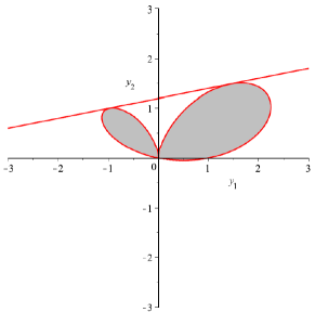
Figure 1. The semialgebraic set $S$ (gray) in Example 3.7 and the line $x_{1}^{*}y_{1}+x_{2}^{*}-y_{2}=0$ (red).

Although the optimal value $p^{*}$ of (1.1) can be approximated by solving the dual problem (2.2) with the SDP relaxations (2.4) given in [23], the hierarchy of SDP relaxations (3.5) of (1.1) itself is of independent interest. For example, we can solve the relaxation $(\ref{eq::psdplsipp})$ and extract the optimal solution $(x^{(k)},Z_{0}^{(k)},\ldots,Z_{s}^{(k)})$ (if it exists) by the software YALMIP [27]. As $p^{\mbox{\tiny sos}}_{k}$ may not be attainable, let $(\tilde{x}^{(k)},\tilde{Z}_{0}^{(k)},\ldots,\tilde{Z}_{s}^{(k)})$ be an $\frac{\varepsilon}{2}$-optimal solution of (3.5). Since $\tilde{x}^{(k)}$ is feasible for (1.1) and $p^{\mbox{\tiny sos}}_{k}-p^{*}<\frac{\varepsilon}{2}$ for some $k\in\mathbb{N}$, a subsequence of $\{\tilde{x}^{(k)}\}_{k\in\mathbb{N}}$ converges to an $\varepsilon$-optimal solution of (1.1) if the feasible set of (1.1) is bounded.

Example 3.8.

Consider the following problem

(3.9) $$\left\{\begin{aligned} \min_{x_{0},x_{i_{1},i_{2}}\in{\mathbb{R}}}&\ x_{0}\\ \text{s.t.}&\ \left|\sum_{i_{1}=0}^{t}\sum_{i_{2}=0}^{t}x_{i_{1},i_{2}}y_{1}^{i_{1}}y_{2}^{i_{2}}-b(y)\right|\leq x_{0},\quad\forall y\in[-1,1]^{2},\\ \end{aligned}\right.$$

which is to approximate the function $b(Y)$ from the spans of $Y_{1}^{i_{1}}Y_{2}^{i_{2}}$ in some sense. Hence, it is more useful to give the minimizers $x^{*}$ which are the corresponding optimal coefficients for the basis functions $Y_{1}^{i_{1}}Y_{2}^{i_{2}}$ in the approximations. Here, we consider two cases [45]:

$$\text{(i):}\ t=2,\ b(Y)=\frac{1}{Y_{1}+2Y_{2}+4};\quad\text{and\ (ii):}\ t=2,\ b(Y)=\sqrt{Y_{1}+2Y_{2}+4}.$$

While $b(Y)$ in (ii) is a semialgebraic function, (3.5) still works by adding some lifted variables, see Section 4.1. Solving (3.5) with YALMIP, the obtained coefficients are listed below

$$\text{(i)}: (0.2341,-0.0468,-0.1507,0.1203,-0.0706,-0.1292,0.0837,0.0136,0.0927),$$

$$\text{(ii)}: (2.0043,0.2494,0.5125,-0.0747,0.0194,0.0350,-0.0133,-0.0178,-0.0708),$$

in the order $(x^{*}_{0,0},x^{*}_{1,0},x^{*}_{0,1},x^{*}_{1,1},x^{*}_{2,1},x^{*}_{1,2},x^{*}_{2,2},x^{*}_{2,0},x^{*}_{0,2})$. $\square$

At the end of this part, let us briefly introduce the SDP relaxation method for general SIPP problems given in [44] which can also be used to solve (1.1). The approach in [44] is based on the following exchange scheme. At its $k$-th iteration, we solve the linear programming problem

(3.10) $$\min_{x\in{\mathbb{R}}^{m}}\ \ c^{T}x\quad\text{s.t.}\ a(y)^{T}x+b(y)\geq 0,\ y\in Y_{k},$$

where $Y_{k}\subset S$ is a finite set and generated at the last iteration. Next, choose a minimizer $x^{(k)}$ of (3.10) and globally solve the polynomial optimizaion problem

(3.11) $$\min_{y\in S}\ \ a(y)^{T}x^{(k)}+b(y)$$

by Lasserre’s SDP relaxation method [21]. Extract the set $\mathcal{S}_{k}$ of global minimizers of (3.11) and let $Y_{k+1}=Y_{k}\cup\mathcal{S}_{k}$, then go to next iteration. To guarantee the convergence, the feasible set of (1.1) need to be compact and $\mathcal{S}_{k}\neq\emptyset$ for each $k$. However, if the flat extension condition or flat trucation condition is not satisfied when solving (3.11) by Lasserre’s relaxation (when $\mathcal{S}_{k}$ is infinite, for example), it is hard to obtain the set $\mathcal{S}_{k}$ without which the iteration goes into dead loop.

3.2. Convergence rate analysis

Denote by $\mathcal{F}$ and $\mathcal{F}_{k}$ the feasible sets of (1.1) and (3.5), respectively. In this subsection, we assume that $\mathcal{F}$ and $S$ are compact. For the simplicity in the convergence rate analysis of the SDP relaxations (3.5), we consider the following assumption which holds possibly after some rescaling.

Assumption 3.9.

It holds that $\mathcal{F}\subseteq(-1,1)^{m}$ and $S\subseteq(-1,1)^{n}$ for (1.1).

Let

$$\omega:=\max\{\deg(a_{1}),\ldots,\deg(a_{m}),\deg(b)\}.$$

For a polynomial $h(Y)=\sum_{\alpha}h_{\alpha}Y^{\alpha}\in{\mathbb{R}}[Y]$, define the norm

$$\|h\|:=\max_{\alpha}\frac{|h_{\alpha}|}{\tbinom{\|\alpha\|_{1}}{\alpha}}.$$

Recalling the proof of Theorem 3.2, we have

Theorem 3.10.

Suppose that Assumption 3.9 holds, $\mathcal{Q}(G)$ is Archimedean and $\bar{x}$ is a Slater point of (1.1). Let $r_{\bar{x}}^{*}:=\min_{y\in S}a(y)^{T}\bar{x}+b(y)>0$, then there exists $\gamma>0$ depending on $g_{i}$’s in (1.2) such that for any $\varepsilon>0$, it holds that $0\leq p_{k}^{\mbox{\tiny sos}}-p^{*}\leq\varepsilon$ whenever

$$k\geq\gamma\exp\left[\left(\omega^{2}n^{\omega}\frac{\sum_{i=1}^{m}\|a_{i}\|+\|b\|}{\kappa(\varepsilon)r_{\bar{x}^{*}}}\right)^{\gamma}\right],$$

where $\kappa(\varepsilon):=\min\{1,\frac{\varepsilon}{4\sqrt{m}\|c\|_{2}}\}$.

Proof.

If $c^{T}\bar{x}-p^{*}\leq\varepsilon$, let $x^{(\varepsilon)}=\bar{x}$; otherwise, let $x^{(\varepsilon)}=\hat{x}$ as defined in (3.2). As $\mathcal{F}\subseteq(-1,1)^{m}$, we have $\delta\geq\frac{\varepsilon}{4\sqrt{m}\|c\|_{2}}$ in (3.2). In either case, it holds from (3.3) that $a(y)^{T}x^{(\varepsilon)}+b(y)\geq\kappa(\varepsilon)r_{\bar{x}^{*}}>0$ for any $y\in S$. By [35, Theorem 6], there exists $\gamma>0$ depending on $g_{i}$’s such that $a(Y)^{T}x^{(\varepsilon)}+b(Y)\in\mathcal{Q}_{\bar{k}}(G)$ where

$$\bar{k}:=\gamma\exp\left[\left(\omega^{2}n^{\omega}\frac{\|a(Y)^{T}x^{(\varepsilon)}+b(Y)\|}{\min_{y\in S}a(y)^{T}x^{(\varepsilon)}+b(y)}\right)^{\gamma}\right].$$

Clearly,

$$\bar{k}\leq\gamma\exp\left[\left(\omega^{2}n^{\omega}\frac{\sum_{i=1}^{m}\|a_{i}\|+\|b\|}{\kappa(\varepsilon)r_{\bar{x}^{*}}}\right)^{\gamma}\right]\leq k.$$

Hence, $a(Y)^{T}x^{(\varepsilon)}+b(Y)\in\mathcal{Q}_{k}(G)$ and $p_{k}^{\mbox{\tiny sos}}-p^{*}\leq c^{T}x^{(\varepsilon)}-p^{*}\leq\varepsilon$ by (3.4). ∎

For any $\varepsilon>0$, compared with (1.1), consider the problem

(3.12) $$(P_{\varepsilon})\qquad\left\{\begin{aligned} p^{*}_{\varepsilon}:=\inf_{x\in{\mathbb{R}}^{m}}&\ c^{T}x\\ \text{s.t.}&\ a(y)^{T}x+b(y)\geq\varepsilon,\ \ \forall y\in S.\end{aligned}\right.$$

Obviously, $p^{*}\leq p^{*}_{\varepsilon}$ for any $\varepsilon>0$. Moreover, by the stability of optimal values of linear semi-infinite programming problems (c.f. [12, Theorem 5.1.5]), it follows that

Lemma 3.11.

If Assumption 3.9 and the Slater condition hold for (1.1), then there exist scalars $\bar{\varepsilon}>0$ and $L>0$ such that $p^{*}_{\varepsilon}-p^{*}\leq L\varepsilon$ for any $\varepsilon\leq\bar{\varepsilon}$.

Proof.

Since $\mathcal{F}$ is compact, the optimal solution set of (1.1) is non-empty and compact. As $S$ is compact, a Slater point of (1.1) is also a strong Slater point. Then, the conclusion follows by the Lipschitz continuity of the optimal value function of (1.1) (see, [12, Theorem 5.1.5]). ∎

For any $\varepsilon>0$, denote the feasible set of (3.12) by

$$\mathcal{F}_{\varepsilon}:=\{x\in{\mathbb{R}}^{m}\mid a(y)^{T}x+b(y)\geq\varepsilon,\quad\forall\ y\in S\}.$$

Lemma 3.12.

Suppose that Assumption 3.9 holds and $\mathcal{Q}(G)$ is Archimedean. Then, there exists some $\gamma>0$ depending on $g_{i}$’s in (1.2) such that for all integers $k>\gamma\exp((2\omega^{2}n^{\omega})^{\gamma})$, we have $\mathcal{F}_{\varepsilon}\subseteq\mathcal{F}_{k}$ whenever

(3.13) $$\varepsilon\geq\varepsilon_{k}:=\frac{6\omega^{3}n^{2\omega}(\sum_{i=1}^{m}\|a_{i}\|+\|b\|)}{\sqrt[\gamma]{\log\frac{k}{\gamma}}}.$$

Proof.

Fix a point $u\in\mathcal{F}_{\varepsilon}$. Let $r_{u}^{*}:=\min_{y\in S}a(y)^{T}u+b(y)$. Then, by [35, Theorem 8], there exists some $\gamma>0$ depending on $g_{i}$’s such that for all $k>\gamma\exp((2\omega^{2}n^{\omega})^{\gamma})$, it holds that

$$a(Y)^{T}u+b(Y)-r_{u}^{*}+\frac{6\omega^{3}n^{2\omega}\|a(Y)^{T}u+b(Y)\|}{\sqrt[\gamma]{\log\frac{k}{\gamma}}}\in\mathcal{Q}_{k}(G).$$

As $u\in\mathcal{F}_{\varepsilon}$, we have $r_{u}^{*}\geq\varepsilon$. Since $\mathcal{F}_{\varepsilon}\subseteq\mathcal{F}$, the assumption $\mathcal{F}\subseteq(-1,1)^{m}$ implies that $\|a(Y)^{T}u+b(Y)\|\leq\sum_{i=1}^{m}\|a_{i}(Y)\|+\|b(Y)\|$. Consequently,

$$r_{u}^{*}-\frac{6\omega^{3}n^{2\omega}\|a(Y)^{T}u+b(Y)\|}{\sqrt[\gamma]{\log\frac{k}{\gamma}}}\geq\varepsilon-\varepsilon_{k}\geq 0.$$

Hence, we have $a(Y)^{T}u+b(Y)\in\mathcal{Q}_{k}(G)$ and $u\in\mathcal{F}_{k}$. ∎

Theorem 3.13.

Suppose that Assumption 3.9, the Slater condition hold for (1.1) and $\mathcal{Q}(G)$ is Archimedean. Then, there exist some $\gamma>0$ depending on $g_{i}$’s in (1.2) and scalars $\bar{\varepsilon}>0$, $L>0$ such that for all integers

$$k>\max\left\{\gamma\exp((2\omega^{2}n^{\omega})^{\gamma}),\ \gamma\exp\left[\frac{6\omega^{3}n^{2\omega}(\sum_{i=1}^{m}\|a_{i}\|+\|b\|)}{\bar{\varepsilon}}\right]^{\gamma}\right\},$$

it holds that

$$0\leq p^{\mbox{\tiny sos}}_{k}-p^{*}\leq L\frac{6\omega^{3}n^{2\omega}(\sum_{i=1}^{m}\|a_{i}\|+\|b\|)}{\sqrt[\gamma]{\log\frac{k}{\gamma}}}.$$

Proof.

Note that all assumptions in Lemma 3.11 and 3.12 hold. Then, there exist $\gamma>0$ depending on $g_{i}$’s, $\bar{\varepsilon}>0$ and $L>0$ as described in the conclusions of Lemma 3.11 and 3.12. Recall $\varepsilon_{k}$ defined in (3.13). By Lemma 3.12, it holds that $\mathcal{F}_{\varepsilon_{k}}\subseteq\mathcal{F}_{k}$ which implies $p^{*}_{\varepsilon_{k}}\geq p^{\mbox{\tiny sos}}_{k}$. Moreover, it is easy to check that $\varepsilon_{k}\leq\bar{\varepsilon}$ and hence $p_{\varepsilon_{k}}^{*}-p^{*}\leq L\varepsilon_{k}$ by Lemma 3.11. Consequently, $p_{k}^{\mbox{\tiny sos}}-p^{*}\leq L\varepsilon_{k}$. ∎

3.3. On compactness of $\mathcal{F}$

In the last subsection, we assume that the feasible set $\mathcal{F}$ of (1.1) is compact in order to estimate the convergence rate of the SDP relaxations (3.5). In the following, we show that the compactness of $\mathcal{F}$ can be determined by solving some LSIPP problems, which can be done by the SDP relaxations (3.5) in some cases. Denote by $\mathbf{0}$ the vector of all zeros in ${\mathbb{R}}^{n}$. In this subsection, without loss of generality,we assume that

Assumption 3.14.

$\mathbf{0}\in\mathcal{F}$, or equivalently, $b(y)\geq 0$ for all $y\in S$.

Denote by $0^{+}\mathcal{F}\subset{\mathbb{R}}^{m}$ the recession cone of $\mathcal{F}$, i.e., $u\in 0^{+}\mathcal{F}$ if and only if $x+tu\in\mathcal{F}$ for all $x\in\mathcal{F}$ and $t\geq 0$. As $\mathcal{F}$ is closed and convex, $\mathcal{F}$ is compact if and only if $0^{+}\mathcal{F}=\{\mathbf{0}\}$ by [40, Theorem 8.4].

Consider the minimax problem

(3.14) $$r_{a}^{*}:=\max_{\|u\|_{2}=1}\min_{y\in S}\ a(y)^{T}u$$

Proposition 3.15.

Suppose that Assumption 3.14 holds for (1.1). Then, its feasible set $\mathcal{F}$ is compact if and only if $r_{a}^{*}<0$.

Proof.

As $\mathbf{0}\in\mathcal{F}$, by [40, Theorem 8.3], a vector $u\in 0^{+}\mathcal{F}$ if and only if $tu\in\mathcal{F}$ for all $t\geq 0$. That is, $(a(y)^{T}u)\cdot t+b(y)\geq 0$ for all $y\in S$ and $t\geq 0$, which is true if and only if $a(y)^{T}u\geq 0$ for all $y\in S$ since $b(y)\geq 0$ on $S$. Note that since $S$ is compact, $\min_{y\in S}\ a(y)^{T}u$ is continuous in $u$ and then $r_{a}^{*}$ is attainable. Therefore, if $\mathcal{F}$ is compact, then $u\not\in 0^{+}\mathcal{F}$ for any nonzero $u\in{\mathbb{R}}^{n}$ and hence $r_{a}^{*}<0$. Conversely, assume that $r_{a}^{*}<0$. If $u\in 0^{+}\mathcal{F}$ for some nonzero $u\in{\mathbb{R}}^{n}$, then we have $r_{a}^{*}\geq 0$, a contradiction. Then, $0^{+}\mathcal{F}=\{\mathbf{0}\}$ and hence $\mathcal{F}$ is compact. ∎

It is clear that the minimax problem (3.14) is equivalent to the following problem

(3.15) $$\left\{\begin{aligned} r_{a}^{*}=\sup_{\|u\|_{2}=1,\lambda\in{\mathbb{R}}}&\ \lambda\\ \text{s.t.}&\ a(y)^{T}u-\lambda\geq 0,\quad\forall\ y\in S.\end{aligned}\right.$$

By some rescalings, we can reformulate the problem (3.15) as the following LSIPP problems of the form (1.1):

$$(P_{i}^{+})\qquad\left\{\begin{aligned} r_{a,i}^{+}:=\inf_{u_{i}=1,\lambda\in{\mathbb{R}}}&\ -\lambda\\ \text{s.t.}&\ a(y)^{T}u-\lambda\geq 0,\ \ \forall y\in S,\end{aligned}\right.$$

and

$$(P_{i}^{-})\qquad\left\{\begin{aligned} r_{a,i}^{-}:=\inf_{u_{i}=-1,\lambda\in{\mathbb{R}}}&\ -\lambda\\ \text{s.t.}&\ a(y)^{T}u-\lambda\geq 0,\ \ \forall y\in S,\end{aligned}\right.$$

for $i=1,\ldots,m$. Then,

Corollary 3.16.

Suppose that Assumption 3.14 holds for (1.1). Then, its feasible set $\mathcal{F}$ is compact if and only if $\min\{r_{a,i}^{+},\ r_{a,i}^{-},\ i=1,\ldots,m\}>0$.

Consequently, the compactness of $\mathcal{F}$ can be verified by a positive lower bound of $\min\{r_{a,i}^{+},\ r_{a,i}^{-},\ i=1,\ldots,m\}$ which can be obtained by solving $(P^{+}_{i})$’s and $(P^{-}_{i})$’s using, for instance, discretization methods.

Note that the SDP relaxations (3.5) and (2.4) produce upper bounds of $p^{*}$ of (1.1). The compactness of $\mathcal{F}$ can also be verified by these SDP relaxations of $(P^{+}_{i})$’s and $(P^{-}_{i})$’s if finite convergence happens for each problem, which can be detected by the flat extension condition (or the weaker flat truncation condition in Remark 3.6). In particular, when $S$ is a closed and bounded interval, the SDP relaxations (3.5) and (2.4) of the smallest order are exact for (1.1) by the representation result of nonnegative polynomials in the univariate case. This result has been investigated in [46]. Precisely, without loss of generality, we can assume that $S=[-1,1]$. Let

$$[-1,1]=\{y_{1}\in{\mathbb{R}}\mid g_{1}(y_{1})\geq 0\},\quad\text{where}\quad g_{1}(Y_{1})=1-Y_{1}^{2}.$$

Recall the well-known result

Theorem 3.17.

(c.f. [26, 38]) Let $h\in{\mathbb{R}}[Y_{1}]$ and $h\geq 0$ on $[-1,1]$, then $h=\sigma+\sigma_{1}(1-Y_{1}^{2})$ where $\sigma,\sigma_{1}\in\Sigma^{2}[Y_{1}]$ and $\deg(\sigma)$, $\deg(\sigma_{1}(1-Y_{1}^{2}))\leq 2\lceil\deg(h)/2\rceil$.

It follows that $p^{\mbox{\tiny sos}}_{k_{P}}=p^{\mbox{\tiny mom}}_{k_{P}}=p^{*}$ holds for (3.5) and (2.4) in this case [46]. Therefore, the compactness of $\mathcal{F}$ can always be verified by SDP relaxations (3.5) and (2.4) of $(P^{+}_{i})$’s and $(P^{-}_{i})$’s when $S$ is a closed and bounded interval.

Example 3.7 revisited. Consider the feasible set $\mathcal{F}$ of (3.8) in Example 3.7, which is clearly noncompact. Note that $\mathbf{0}\not\in\mathcal{F}$ and we have proved that the minimizer is $(\frac{1}{5},\frac{125}{104})$. Let $w_{1}=x_{1}-\frac{1}{5}$, $w_{2}=x_{2}-\frac{125}{104}$ and move the set $\mathcal{F}$ to

$$\left\{w\in{\mathbb{R}}^{2}\mid\left(w_{1}+\frac{1}{5}\right)y_{1}+\left(w_{2}+\frac{125}{104}\right)-y_{2}\geq 0,\ \forall\ y\in S\right\},$$

which contains $\mathbf{0}$. Consider the LSIPP problem

$$(P_{1}^{+})\qquad\left\{\begin{aligned} r_{a,1}^{+}:=\inf_{u_{2},\lambda\in{\mathbb{R}}}&\ -\lambda\\ \text{s.t.}&\ y_{1}+u_{2}-\lambda\geq 0,\ \ \forall y\in S.\end{aligned}\right.$$

It is easy to check that $y_{1}\geq-2$ for all $y\in S$. Then, $(u_{2}=N+2,\lambda=N)$ is feasible for $(P_{1}^{+})$ for all $N\in\mathbb{N}$. Hence, we have $r_{a,1}^{+}=-\infty$ and therefore $\mathcal{F}$ is noncompact by Corollary 3.16. $\square$

Example 3.19.

Consider the ellipse

$$\mathcal{F}:=\{(x_{1},x_{2})\in{\mathbb{R}}^{2}\mid 2x_{1}^{2}+x_{2}^{2}+2x_{1}x_{2}+2x_{1}\leq 0\}$$

which can be represented by

$$\{(x_{1},x_{2})\in{\mathbb{R}}^{2}\mid a(y_{1})^{T}x+b(y_{1})\geq 0,\ \forall y_{1}\in S\}$$

where

$$a(Y_{1})=(-Y_{1}^{4}-2Y_{1}^{3}+3Y_{1}^{2}+2Y_{1}-1,-2Y_{1}(Y_{1}^{2}-1))^{T},\quad b(Y_{1})=2Y_{1}^{2},$$

and $S=[-1,1]$ $($see [11]$)$. Clearly, $\mathcal{F}$ is compact and $\mathbf{0}\in\mathcal{F}$. As $S=[-1,1]$, all problems $(P^{+}_{i})$’s and $(P^{-}_{i})$’s can be solved by the SDP relaxations (3.5) and (2.4) of order $d_{P}=2$. Using GloptiPoly, we first solve the SDP relaxation (2.4) of

$$(P_{1}^{+})\qquad\left\{\begin{aligned} r_{a,1}^{+}:=\inf_{u_{2},\lambda\in{\mathbb{R}}}&\ -\lambda\\ \text{s.t.}&\ -y_{1}^{4}-2y_{1}^{3}+3y_{1}^{2}+2y_{1}-1-2y_{1}(y_{1}^{2}-1)u_{2}-\lambda\geq 0,\\ &\ \forall y_{1}\in S.\end{aligned}\right.$$

As the infeasibility of the SDP problem is detected by the SDP solver SeDuMi [42] called by GloptiPoly, we have $r_{a,1}^{+}=+\infty$. We continue to solve $(P_{1}^{-})$, $(P_{2}^{+})$ and $(P_{2}^{-})$. The results solved by GloptiPoly are $r_{a,1}^{-}=1$, $r_{a,2}^{+}=0.5491$ and $r_{a,2}^{-}=0.7698$, which imply the compactness of $\mathcal{F}$ by Corollary 3.16. $\square$

Note that the index set $S$ is required to be compact to guarantee the convergence of the SDP relaxations (3.5) and (2.4). To end this section, we consider two examples to illustrate how to deal with the case when $S$ is noncompact by the homogenization technique and its applications in polynomial optimzation problems.

Example 3.20.

Consider the LSIPP problem

(3.16) $$p^{*}:=\inf_{x\in{\mathbb{R}}}\ -\frac{x}{2}\quad\text{s.t.}\ (1-3y_{2})x+3y_{1}\geq 0,\ \forall y\in S,$$

where

$$S:=\{y\in{\mathbb{R}}^{2}\mid y_{1}\geq 0,y_{1}^{2}-y_{2}^{3}\geq 0\}.$$

Since $(0,0)\in S$, a feasible $x$ must be nonnegative. Clearly, $x=0$ is a feasible point. $x>0$ is feasible if and only if

$$0\geq\max_{y\in S}\left\{y_{2}-\frac{1}{3}-\frac{y_{1}}{x}\right\}=\max_{y\in S}\left\{y_{1}^{\frac{2}{3}}-\frac{1}{3}-\frac{y_{1}}{x}\right\}.$$

The latter maximum is attained at $\frac{8x^{3}}{27}$ with optimal value $\frac{4x^{2}}{27}-\frac{1}{3}$. Thus, the feasible set of (3.16) is $[0,\frac{3}{2}]$ and the minimizer is $x^{*}=\frac{3}{2}$.

Obviously, $\mathcal{Q}(G)$ is not Archimedean. For any $k\in\mathbb{N}$, we know from [13, Example 2.10] that $(1-3Y_{2})x+3Y_{1}\in\mathcal{Q}_{k}(G)$ if and only if $x=0$, i.e., $p^{\mbox{\tiny sos}}_{k}=0$ for each $k\geq d_{P}$. Now we show that $p^{\mbox{\tiny mom}}_{k}=p^{\mbox{\tiny sos}}_{k}$ for each $k\geq d_{P}$. In fact, for the SDP relaxation $(\ref{eq::dsdplsipp})$ of the problem $(\ref{eq::counterex})$, let $\mu$ be a probability measure with uniform distribution in the following subset of $S$:

$$S_{1}:=\{(y_{1},y_{2})\in{\mathbb{R}}^{2}\mid 1\leq y_{1}\leq 2,\ 0\leq y_{2}\leq 1\}$$

and $z^{(\mu)}$ be the truncated moment sequence with representing measure $\mu$ up to order $2k$. It can be verified that $z^{(\mu)}$ is a feasible point of $(\ref{eq::dsdplsipp})$ and its corresponding truncated moment matrix and localizing moment matrices are positive definite since $S_{1}$ has nonempty interior. Then $p^{\mbox{\tiny mom}}_{k}=p^{\mbox{\tiny sos}}_{k}$ follows by the conic duality theorem. Hence, both SDP relaxations $(\ref{eq::psdplsipp})$ and $(\ref{eq::dsdplsipp})$ do not converge to the optimum.

Now let us see how to solve this issue by homogenization. We first homogenize the defining polynomials of $S$ by new variable $y_{0}$ and define the following bounded set

$$\widetilde{S}_{>} :=\{\tilde{y}=(y_{0},y_{1},y_{2})\in{\mathbb{R}}^{3}\mid y_{1}\geq 0,\ y_{0}y_{1}^{2}-y_{2}^{3}\geq 0,\ y_{0}>0,\ \|\tilde{y}\|_{2}^{2}=1\}.$$

Then, we homogenize the constraint polynomial of (3.16) with respect to $Y$ and consider the problem

$$\inf_{x\in{\mathbb{R}}}\ -\frac{x}{2}\quad\text{s.t.}\ (y_{0}-3y_{2})x+3y_{1}\geq 0,\ \forall\tilde{y}=(y_{0},y_{1},y_{2})\in{\sf closure}(\widetilde{S}_{>}),$$

which is equivalent to (3.16) by [44, Proposition 4.2]. However, the set ${\sf closure}(\widetilde{S}_{>})$ is not in the form of basic semialgebraic sets. Hence, we define the following compact set

$$\widetilde{S}:=\{(y_{0},y_{1},y_{2})\in{\mathbb{R}}^{3}\mid y_{1}\geq 0,\ y_{0}y_{1}^{2}-y_{2}^{3}\geq 0,\ y_{0}\geq 0,\ \|\tilde{y}\|_{2}^{2}=1\}.$$

We say $S$ is closed at $\infty$ [33] if $\widetilde{S}={\sf closure}(\widetilde{S}_{>})$, in which case (3.16) is equivalent to

(3.17) $$\inf_{x\in{\mathbb{R}}}\ -\frac{x}{2}\quad\text{s.t.}\ (y_{0}-3y_{2})x+3y_{1}\geq 0,\ \forall\tilde{y}=(y_{0},y_{1},y_{2})\in\widetilde{S}.$$

Note that $S$ is indeed closed at $\infty$. In fact, for every $(0,v_{1},v_{2})\in\widetilde{S}\backslash\widetilde{S}_{>}$, let

$$v^{(\varepsilon)}:=\left(\varepsilon,\ v_{1},\ \sqrt[3]{\varepsilon v_{1}^{2}+v_{2}^{3}}\right).$$

Then $\{v^{(\varepsilon)}/\|v^{(\varepsilon)}\|_{2}\}_{\varepsilon>0}\subseteq\widetilde{S}_{>}$ and $\lim_{\varepsilon\rightarrow 0}v^{(\varepsilon)}/\|v^{(\varepsilon)}\|_{2}=(0,v_{1},v_{2})$. Hence, we have $\widetilde{S}\backslash\widetilde{S}_{>}\subseteq{\sf closure}(\widetilde{S}_{>})$ and so $S$ is closed at $\infty$. Clearly, the quadratic module associated with $\widetilde{S}$ is Archimedean and $\bar{x}=1$ is a Slater point of $(\ref{eq::counterex2})$. With GloptiPoly, we solve the SDP relaxations (2.4) of (3.17) and get the following numerical results: $p_{2}^{\mbox{\tiny mom}}=-1.2124\times 10^{-8}$ and $p_{3}^{\mbox{\tiny mom}}=-0.7500$. The flat extension condition is satisfied for $k=3$ and we obtain the certified optimum $-0.7500$. By Proposition 3.5, the extracted numerical active index set of the minimizer $x^{*}=3/2$ is ${(0.5773,0.5774,0.5774)}$ which corresponds to $(1,1)\in S$. $\square$

Remark 3.21.

Note that not every set $S$ of the form $(\ref{eq::S})$ is closed at $\infty$ even when it is compact [31, Example 5.2]. However, it is shown in [44, Theorem 4.10] that the closedness at $\infty$ is a generic property.

Example 3.22.

Consider the following polynomial optimization problem

(3.18) $$\left\{\begin{aligned} \inf_{y\in{\mathbb{R}}^{2}}&\ \ f(y):=y_{1}^{2}+y_{2}^{2}\\ \text{s.t.}&\ \ y\in S:=\{y\in{\mathbb{R}}^{2}\mid g_{1}(y)\geq 0,\ g_{2}(y)\geq 0,\ g_{3}(y)\geq 0\},\end{aligned}\right.$$

where

$$g_{1}(Y)=Y_{2}^{2}-1,\ g_{2}(Y)=Y_{1}^{2}-Y_{1}Y_{2}-1,\ g_{3}(Y)=Y_{1}^{2}+Y_{1}Y_{2}-1.$$

It was shown in [8, 29, 33] that the global minimizers and global minimum are

$$\left(\pm\frac{1+\sqrt{5}}{2},\pm 1\right)\approx(\pm 1.618,\pm 1)\quad\text{and}\quad 2+\frac{(1+\sqrt{5})}{2}\approx 3.618.$$

Because $S$ is noncompact, the classic Lasserre’s SDP relaxations [21] of $(\ref{eq::stable})$ can only provide lower bounds $2$ no matter how large the order is (c.f. [8]).

Clearly, any polynomial optimization problem of the form (3.18) can be equivalently reformulated to the following LSIPP problem

(3.19) $$f^{*}=\sup_{x\in{\mathbb{R}}}\ \ x\quad\text{s.t.}\ \ f(y)-x\geq 0,\ \forall y\in S.$$

As $S$ is noncompact, we use the homogenization technique in Example 3.20 to convert this LSIPP problem to

(3.20) $$\tilde{f}^{*}:=\sup_{x\in{\mathbb{R}}}\ \ x\quad\text{s.t.}\ \ f^{h}(\tilde{y})-xy_{0}^{\deg(f)}\geq 0,\ \forall\tilde{y}\in\widetilde{S},$$

where $f^{h}$ is the homogenization of $f$ and $\widetilde{S}$ is defined as in Example 3.20. Suppose that $f^{*}>-\infty$, then the Slater condition holds for (3.20) if and only if

(3.21) $$\hat{f}(y)>0,\quad\forall\ y\in\widehat{S}:=\{y\in{\mathbb{R}}^{n}\mid\hat{g}_{1}(y)\geq 0,\ \ldots,\ \hat{g}_{s}(y)\geq 0,\ \|y\|_{2}^{2}=1\},$$

where $\hat{f}$ and $\hat{g}_{i}$’s are the homogeneous parts of $f$ and $g_{i}$’s of the highest degree. Moreover, if the condition (3.21) holds for (3.20), it is easy to see that any feasible point of (3.19) is also feasible for (3.20). Thus, $\tilde{f}^{*}=f^{*}$ and we can compute them by the SDP relaxations (3.5) and (2.4).

Obviously, the condition (3.21) holds for (3.18). We compute the relaxations (2.4) of (3.20) with GloptiPoly. For $k=3$, the flat extension condition is satisfied and we get the numerically certified optimum $f^{\mbox{\tiny mom}}_{3}=3.6180$. The extracted active index set is $\{(0.4653,\pm 0.7529,\pm 0.4653)\}$ which corresponds to the set of global minimizers $(\pm 1.6181,\pm 1)$. $\square$

Remark 3.23.

(i) By [30, Theorem 5.1 and 5.3], the condition (3.21) holds if and only if $f$ is stably bounded from below on $S$, i.e., $f$ remains bounded from below on $S$ for all sufficiently small perturbations of the coefficients of $f,g_{1},\ldots,g_{s}$. Therefore, we give an SDP relaxation method in Example 3.22 for solving the class of polynomial optimization problems whose objective polynomials are stably bounded from below on noncompact feasible sets; (ii) Note that the stably boundedness from below of $f$ on $S$ is irrelevant to the closedness at $\infty$ of $S$. For example, the set $\{y\in{\mathbb{R}}^{2}\mid y_{2}\geq y_{1}^{2}\}$ is not closed at $\infty$ but $Y_{2}^{2}$ is stably bounded from below on it; the set $S$ in Example 3.20 is closed at $\infty$ but $Y_{1}$ is not stably bounded from below on it.

4. Some extensions

In this section, we discuss some extensions of the SDP relaxations (3.5) for (1.1) in Section 3 to more general semi-infinite programming problems.

4.1. LSIP with semi-algebraic functions

Inspired by Lasserre and Putinar’s work [25], we would like to point out that the SDP relaxation method proposed in this paper is applicable to a more general subclass of LSIP problems. Denote by $\mathcal{X}\subseteq{\mathbb{R}}^{m}$ a convex polyhedron defined by finitely many linear inequalities in the variables $X$. Denote by $\mathcal{A}$ the algebra consisting of functions generated by finitely many of the dyadic operations $\{+,-,/,\vee,\wedge\}$ and monadic operations $\{|\cdot|,(\cdot)^{1/p},p\in\mathbb{N}\}$ on polynomials in ${\mathbb{R}}[Y]$, where $f\vee g:=\max[f,g]$ and $f\wedge g:=\min[f,g]$ for $f,g\in{\mathbb{R}}[Y]$. For example,

$$\sqrt{|f(Y)|+g(Y)^{2}}\wedge\left(\frac{1}{g(Y)}\vee f(Y)\right)\in\mathcal{A}.$$

Note that every function in $\mathcal{A}$ has a lifted basic semi-algebraic representation [25, Definition 1]. Then, the SDP relaxations (3.5) and (2.4) can be extended for more general LSIP problems of the form

(4.1) $$\left\{\begin{aligned} p^{*}:=\inf_{x\in\mathcal{X}}&\ c^{T}x\\ \text{s.t.}&\ a^{l}(y)^{T}x+b_{l}(y)\geq 0,\ \ \forall y\in S\text{ and }l=1,\ldots,t,\end{aligned}\right.$$

where $c\in{\mathbb{R}}^{m}$, $a^{l}(Y)\in\mathcal{A}^{m}$, $b_{l}(Y)\in\mathcal{A}$, $l=1,\ldots,t$ and

(4.2) $$S:=\{y\in{\mathbb{R}}^{n}\mid g_{1}(y)\geq 0,\ldots,g_{s}(y)\geq 0\},$$

where $g_{j}(Y)\in\mathcal{A}$, $j=1,\dots,s$. In fact, as shown in [25], the nonnegativity test of semi-algebraic functions in $\mathcal{A}$ on the set $(\ref{eq::Snew})$ can be reduced to an equivalent polynomial funcation case in a lifted space by adding some new variables. For instance, with $f,h,g_{1},g_{2}\in{\mathbb{R}}[Y_{1}]$,

$$\sqrt{f(y_{1})}-1/h(y_{1})\geq 0\quad\text{on}\quad\{y_{1}\in{\mathbb{R}}\mid|g_{1}(y_{1})|g_{2}(y_{1})\geq 1\}$$

can be written as $y_{2}-y_{3}\geq 0$ on

$$\{y\in{\mathbb{R}}^{4}\mid f(y_{1})=y_{2}^{2},\ y_{2}\geq 0,\ h(y_{1})y_{3}=1,\ y_{4}g_{2}(y_{1})\geq 1,\ g_{1}(y_{1})^{2}=y_{4}^{2},\ y_{4}\geq 0\}.$$

Consequently, the extension to $\mathcal{A}$ of Putinar’s Positivstellensatz ([25, Theorem 2]) provides us representations of each nonnegativity constraint in (4.2) via s.o.s and the dual theory of moments. Notice that the constraint $x\in\mathcal{X}$ is linear in $X$. Hence, SDP relaxations as (3.5) and its dual (2.4) can be similarly derived for (4.1) by lifting the parameter space. Moreover, the convergence results and stopping criterion, as Theorem 3.3, 3.4 and Proposition 3.5, can also be analogously established. As might be expected, additional parameters in the lifted space can cause more computational burden in resulting SDP problems. However, as pointed out in [25], the running intersection property holds true for these lifted parameters. Hence, like for polynomial optimization problems [22, 43], some sparse SDP relaxations for (4.1) can be explored to reduce the computational cost.

Example 4.1.

Consider the one-sided $L_{1}$ approximation problem

(4.3) $$\left\{\begin{aligned} \min_{x\in{\mathbb{R}}^{n}}&\ \sum_{i=1}^{n}\frac{x_{i}}{i}\\ \text{s.t.}&\ \sum_{i=1}^{n}y^{i-1}x_{i}-b(y)\geq 0,\quad\forall y\in[0,1].\end{aligned}\right.$$

Here, we approximate two (semi-algebraic) functions [9] on $[0,1]$:

$$\text{(i):}\ \ b(y)=\frac{1}{2-y},\ n=8;\quad\text{and}\quad\text{(ii):}\ \ b(y)=-\frac{1}{1+y^{2}},\ n=10.$$

Clearly, in order to convert this problem into LSIPP, we can add lifted variable $z$ such that $(2-y)z=1$ for case (i) and $(1+y^{2})z=-1$ for case (ii). Then, we solve the SDP relaxations (3.5) with order $k=4$ for (i) and $k=5$ for (ii) by YALMIP. The obtained coefficients $x_{i}$’s are listed below

(i): $$(0.5000,0.2501,0.1227,0.0787,-0.0258,0.1226,-0.0967,0.0484),$$

(ii): $$(-1.0000,-0.0000,1.0016,-0.0202,-0.8566,-0.6123,2.6222,-2.6059,$$

$$1.1881,-0.2168)$$

We show the accuracy of the computed optimal approximations (denoted by $f$) of $b(Y)$ in Figure 2.

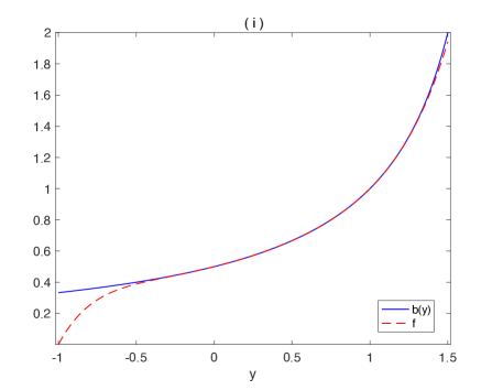
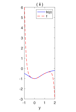
Figure 2. Pictures for the univariate approximation problems in Example 4.1.

Example 4.2.

In $(x_{1},x_{2})$-plane, consider the intersection area $\mathcal{F}$ of $x_{2}\geq 0$, $1-x_{1}^{2}-x_{2}^{2}\geq 0$ and $x_{1}+1-x_{2}^{2}\geq 0$. Then, $\mathcal{F}$ can also be seen as the interstion of $x_{2}\geq 0$, the half planes defined by the lines tangent to $1-x_{1}^{2}-x_{2}^{2}=0$ in the first quadrant and to $x_{1}+1-x_{2}^{2}=0$ in the second quadrant, as shown in Figure 3. Therefore, it is easy to check that

$$\mathcal{F}=\{(x_{1},x_{2})\in{\mathbb{R}}^{2}\mid a(y_{1})^{T}x+b(y_{1})\geq 0,\ \forall\ y_{1}\in[-1,1]\}\cap\mathcal{X},$$

where $\mathcal{X}=\{(x_{1},x_{2})\in{\mathbb{R}}^{2}\mid x_{2}\geq 0\}$,

$$a_{1}(y_{1})=-\min[y_{1},0]-\max[y_{1},0]y_{1},$$

$$a_{2}(y_{1})=2\min[y_{1},0]\sqrt{y_{1}+1}-\max[y_{1},0]\sqrt{1-y_{1}^{2}},$$

$$b(y_{1})=-\min[y_{1},0](2+y_{1})+\max[y_{1},0].$$

Here, the equations $a(y_{1})^{T}X+b(y_{1})=0$ for $y_{1}\in[-1,1]$, in fact, represent the tangent lines mentioned above. Consider the LSIP problem

$$\left\{\begin{aligned} p^{*}:=\min_{x\in\mathcal{X}}&\ c^{T}x\\ \text{s.t.}&\ a(y_{1})^{T}x+b(y_{1})\geq 0,\ \ \forall y\in[-1,1],\end{aligned}\right.$$

in two cases: (i) $c=(1,-1)$; (ii) $c=(-1,-1)$. We can verify that the minima and minimizers are: (i) $p^{*}=-\frac{5}{4}$, $x^{*}=(-\frac{3}{4},\frac{1}{2})$; (ii) $p^{*}=-\sqrt{2}$, $x^{*}=(\frac{\sqrt{2}}{2},\frac{\sqrt{2}}{2})$. Now, we first convert this LSIP problem into LSIPP by the lifting method and then solve it by the SDP relaxations (3.5). As $2\cdot\min[y_{1},0]=y_{1}-|y_{1}|$ and $2\cdot\max[y_{1},0]=y_{1}+|y_{1}|$, we can write

$$\mathcal{F}=\{(x_{1},x_{2})\in{\mathbb{R}}^{2}\mid\tilde{a}(y)^{T}x+\tilde{b}(y)\geq 0,\ \forall\ y\in S\}\cap\mathcal{X},$$

where

$$\tilde{a}_{1}(y) =-y_{1}+y_{2}-y_{1}^{2}-y_{1}y_{2},$$

$$\tilde{a}_{2}(y) =2y_{1}y_{3}-2y_{2}y_{3}-y_{1}y_{4}-y_{2}y_{4},$$

$$\tilde{b}(y) =-(2+y_{1})(y_{1}-y_{2})+y_{1}+y_{2},$$

and

$$S=\{y\in{\mathbb{R}}^{4}\mid-1\leq y_{1}\leq 1,y_{2}^{2}=y_{1}^{2},y_{2}\geq 0,1+y_{1}=y_{3}^{2},y_{3}\geq 0,1-y_{1}^{2}=y_{4}^{2},y_{4}\geq 0\}.$$

Now we can use the SDP relaxations (3.5) to solve the obtained LSIPP problems. The approximate minima and minimizers are: (i) $p_{5}^{\mbox{\tiny sos}}=-1.2496$, $\tilde{x}^{(5)}=(-0.7575,0.4921)$; (ii) $p_{5}^{\mbox{\tiny sos}}=-1.3936$, $\tilde{x}^{(5)}=(0.6544,0.7392)$.

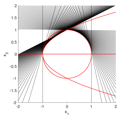
Figure 3. The feasible set $\mathcal{F}$ in Example 4.2.

4.2. S.O.S-convex objectives

Next, by the exact SDP relaxations for classes of nonlinear SDP problems proposed in [18], we extend the SDP relaxation method in Section 3 to the following semi-infinite programming problem

(4.4) $$\left\{\begin{aligned} h^{*}:=\inf_{x\in{\mathbb{R}}^{m}}&\ h(x)\\ \text{s.t.}&\ a(y)^{T}x+b(y)\geq 0,\ \ \forall y\in S,\end{aligned}\right.$$

where $a(Y)$, $b(Y)$, $S$ are defined as in (1.1) and $h(X)\in{\mathbb{R}}[X]$ is s.o.s-convex polynomial. Recall that

Definition 4.3.

([14]) A polynomial $h\in{\mathbb{R}}[Y]$ is s.o.s-convex if its Hessian $\nabla^{2}h$ is a s.o.s, i.e., there are an integer $r$ and a matrix polynomial $H\in{\mathbb{R}}[Y]^{r\times n}$ such that $\nabla^{2}h(Y)=H(Y)^{T}H(Y)$.

While checking the convexity of a polynomial is generally NP-hard [1], s.o.s-convexity can be checked numerically by solving an SDP, see [14].

We first relax (4.4) with arbitrary convex polynomial objective function as

(4.5) $$h^{\mbox{\tiny sos}}:=\inf_{x\in{\mathbb{R}}^{m}}\ \ h(x)\quad\text{s.t.}\ a(Y)^{T}x+b(Y)\in\mathcal{Q}(G).$$

Theorem 4.4.

If $h(X)$ is convex, $\mathcal{Q}(G)$ is Archimedean and the Slater condition holds for (4.4), then $h^{\mbox{\tiny sos}}=h^{*}$.

Proof.

As $h(X)$ is convex, replacing the function $c^{T}X$ in the proof of Theorem 3.2 by $h(X)$, all arguments in the proof of Theorem 3.2 are still valid. In particular, (3.4) become

$$p^{\mbox{\tiny sos}}-p^{*} \leq h(\hat{x})-p^{*}$$

$$\leq(1-\delta)h(x^{\prime})+\delta h(\bar{x})-p^{*}$$

$$=(h(x^{\prime})-p^{*})+\delta(h(\bar{x})-h(x^{\prime}))$$

$$<\frac{\varepsilon}{2}+\frac{\varepsilon}{2}=\varepsilon,$$

due to the convexity of $h$. Then the conclusion follows. ∎

Recall that $\mathcal{F}_{k}$ denotes the feasible set of (3.5). For $k\geq d_{P}$, replacing $\mathcal{Q}(G)$ in $(\ref{eq::sosconvexsip2})$ by its $k$-th truncation $\mathcal{Q}_{k}(G)$, we get

(4.6) $$h_{k}^{\mbox{\tiny sos}}:=\inf\ \ h(x)\quad\text{s.t.}\ x\in\mathcal{F}_{k}.$$

Consequently, it follows from the proof of Theorem 3.3 that

Theorem 4.5.

If $h(X)$ is convex, $\mathcal{Q}(G)$ is Archimedean and the Slater condition holds for (4.4), then $h^{\mbox{\tiny sos}}_{k}$ decreasingly converges to $h^{*}$ as $k\rightarrow\infty$.

Moreover, if $h(X)$ is s.o.s-convex, we point out that for each $k\geq d_{P}$, (4.6) is equivalent to a single SDP problem under certain conditions as shown in [18]. In fact, it is easy to see that there exist some integers $l,t$ and real $t\times t$ symmetric matrices $\{A_{i}\}_{i=0}^{m}$ and $\{B_{j}\}_{j=1}^{l}$ such that $\mathcal{F}_{k}$ is identical with

$$\left\{x\in{\mathbb{R}}^{m}\ \Big{|}\ \exists w\in{\mathbb{R}}^{l},\ \text{s.t.}\ A_{0}+\sum_{i=1}^{m}A_{i}x_{i}+\sum_{j=1}^{l}B_{j}w_{j}\succeq 0\right\},$$

where $w_{j}$’s correspond to the entries of $Z_{j}$’s in (3.6). Thus, (4.6) becomes

(4.7) $$\left\{\begin{aligned} h_{k}^{\mbox{\tiny sos}}=\inf_{x\in{\mathbb{R}}^{m},w\in{\mathbb{R}}^{l}}&\ \ h(x)\\ \text{s.t.}&\ \ A_{0}+\sum_{i=1}^{m}A_{i}x_{i}+\sum_{j=1}^{l}B_{j}w_{j}\succeq 0.\end{aligned}\right.$$

Let $d\in\mathbb{N}$ is the smallest even number such that $d\geq\deg{h}$. Denote the variables $W=(W_{1},\ldots,W_{l})$ and let $\Sigma^{2}_{d}[X,W]$ be the set of sums of squares of polynomials in ${\mathbb{R}}[X,W]$ of degree up to $d$. Consider the dual problem of (4.7)

(4.8) $$\left\{\begin{aligned} \lambda_{k}:=\sup_{\lambda\in{\mathbb{R}},V\in\mathbb{S}_{+}^{m}}&\ \lambda\\ \text{s.t.}&\ h(X)-\sum_{i=1}^{m}\langle A_{i},V\rangle\cdot X_{i}-\sum_{j=1}^{l}\langle B_{j},V\rangle\cdot W_{j}-\langle A_{0},V\rangle-\lambda\\ &\ \in\Sigma^{2}_{d}[X,W],\end{aligned}\right.$$

which can be reduced to an SDP problem as shown in Section 3. Clearly, $h^{\mbox{\tiny sos}}_{k}\geq\lambda_{k}$. We have $h^{\mbox{\tiny sos}}_{k}=\lambda_{k}$ under certain conditions (c.f. [18, Theorem 3.1]). Therefore, an SDP relaxation method is drived for (4.4) with s.o.s-convex objectives.

Example 4.6.

[6] Consider the followin SIP problem

$$\left\{\begin{aligned} h^{*}=\inf_{x\in{\mathbb{R}}^{3}}&\ x_{1}^{2}+x_{2}^{2}+x_{3}^{2}\\ \text{s.t.}&\ -(y_{1}+y_{2}^{2}+1)x_{1}-(y_{1}y_{2}-y_{2}^{2})x_{2}-(y_{1}y_{2}+y_{2}^{2}+y_{2})x_{3}-1\geq 0,\\ &\ \forall y\in[0,1]^{2}.\end{aligned}\right.$$

The exact minimum and minimizer are $h^{*}=1$ and $x^{*}=(-1,0,0)$ [6]. Clearly, the objective function is s.o.s-convex. Solving the SDP problem (4.8), we obtain $\lambda_{1}=1.0000$ with approximate minimizer $(-1.0000,2.3149\times 10^{-6},-1.0410\times 10^{-5})$.

Example 4.7.

Consider the following SIP problem

$$\left\{\begin{aligned} h^{*}=\inf_{x\in{\mathbb{R}}^{2}}&\ h(x)=\frac{5}{8}x_{1}^{2}-4x_{1}+\frac{3}{4}x_{1}x_{2}-4x_{2}+\frac{5}{8}x_{2}^{2}+8\\ \text{s.t.}&\ 1-y_{1}x_{1}-y_{2}x_{2}\geq 0,\ \forall y\in\{y\in{\mathbb{R}}^{2}\mid y_{1}^{2}+y_{2}^{2}=1\}.\end{aligned}\right.$$

Clearly, $h(X)$ is s.o.s-convex. It is easy to see that the feasible set is the closed unit disk around the origin. If we let $f(X)=(X_{1}-2)^{2}+\frac{(X_{2}-2)^{2}}{4}$, then $h(X)=f(\frac{(X_{1}-2)+(X_{2}-2)}{\sqrt{2}}+2,\frac{-(X_{1}-2)+(X_{2}-2)}{\sqrt{2}}+2)$. Geometrically, for any $r>0$, the curve $h(X)=r$ can be obtained by rotating the ellipse $f(X)=r$ around $(2,2)$ by $45^{\circ}$ counterclockwise. Therefore, the minimizer is $x^{*}=(\frac{\sqrt{2}}{2},\frac{\sqrt{2}}{2})$ with the minimum $h^{*}=9-4\sqrt{2}\approx 3.3431$. Solving the SDP problem (4.8), we obtain $\lambda_{1}=3.3432$ with approximate minimizer $(0.7071,0.7071)$.

5. Conclusion

In this paper, a hierarchy of SDP relaxations for LSIPP problems is presented. It can be seen as the dual of Lasserre’s relaxations for GPM problems and enjoys several desirable features. Some (approximate) minimizers of LSIPP problems can be extracted using these SDP relaxations, which is useful in some applications. Convergence rate of these SDP relaxations is estimated using some existing results. We also extend this SDP relaxation method to more general semi-infinite programming problems.

Acknowledgments: The authors are very grateful for the comments of two anonymous referees which helped to improve the presentation. The authors would like to thank Miguel A. Goberna for helpful comments on the Lipschitz continuity of the optimal value function of (1.1) used in Lemma 3.11. Feng Guo is supported by the Chinese National Natural Science Foundation under grants 11401074, 11571350. Xiaoxia Sun is supported by the Chinese National Natural Science Foundation under grant 11801064, the Foundation of Liaoning Education Committee under grant LN2017QN043.

References

- [1] A. A. Ahmadi, A. Olshevsky, P. A. Parrilo, and J. N. Tsitsiklis. NP-hardness of deciding convexity of quartic polynomials and related problems. Mathematical Programming, 137(1):453–476, 2013.
- [2] N. I. Akhiezer. The Classical Moment Problem. Hafner, New York, NY, 1965.
- [3] N. I. Akhiezer and M. G. Krein. Some Questions in the Theory of Moment. American Mathematical Society, Providence, RI, 1962.
- [4] G. A. Anastassiou. Moments in Probability Theory and Approximation Theory. Pitman Research Notes in Mathematics Series. Longman Scientific & Technical, 1993.
- [5] A. Charnes, W. W. Cooper, and K. Kortanek. On representations of semi-infinite programs which have no duality gaps. Management Science, 12(1):113–121, 1965.
- [6] I. D. Coope and G. A. Watson. A projected lagrangian algorithm for semi-infinite programming. Mathematical Programming, 32(3):337–356, 1985.
- [7] R. E. Curto and L. A. Fialkow. Truncated -moment problems in several variables. Journal of Operator Theory, 54(1):189–226, 2005.
- [8] J. Demmel, J. Nie, and V. Powers. Representations of positive polynomials on noncompact semialgebraic sets via KKT ideals. Journal of Pure and Applied Algebra, 209(1):189 – 200, 2007.
- [9] K. Glashoff and S. A. Gustafson. Linear Optimization and Approximation. Springer-Verlag, Berlin, 1983.
- [10] M. Á. Goberna. Linear semi-infinite optimization: Recent advances. In V. Jeyakumar and A. Rubinov, editors, Continuous Optimization, volume 99 of Applied Optimization, pages 3–22. Springer, US, 2005.
- [11] M. Á. Goberna and M. A. López. Linear semi-infinite optimization. John Wiley & Sons, Chichester, 1998.
- [12] M. A. Goberna and M. A. López. Post-Optimal Analysis in Linear Semi-Infinite Optimization. SpringerBriefs in Optimization. Springer, New York, NY, 2014.
- [13] F. Guo, C. Wang, and L. Zhi. Semidefinite representations of noncompact convex sets. SIAM Journal on Optimization, 25(1):377–395, 2015.
- [14] J. Helton and J. Nie. Semidefinite representation of convex sets. Mathematical Programming, 122(1):21–64, 2010.
- [15] D. Henrion and J. B. Lasserre. Detecting global optimality and extracting solutions in gloptipoly. In D. Henrion and A. Garulli, editors, Positive Polynomials in Control, pages 293–310. Springer, Berlin, Heidelberg, 2005.
- [16] D. Henrion, J. B. Lasserre, and J. Löfberg. GloptiPoly 3: moments, optimization and semidefinite programming. Optimization Methods and Software, 24(4-5):761–779, 2009.
- [17] R. Hettich and K. O. Kortanek. Semi-infinite programming: Theory, methods, and applications. SIAM Review, 35(3):380–429, 1993.
- [18] V. Jeyakumar and G. Li. Exact SDP relaxations for classes of nonlinear semidefinite programming problems. Operations Research Letters, 40(6):529 – 536, 2012.
- [19] J. H. B. Kemperman. Geometry of the moment problem. In H. J. Landau, editor, Moments in Mathematics, Proceedings of Symposia in Applied Mathematics 37, pages 16–53. American Mathematical Society, Providence, 1980.
- [20] H. J. Landau. Moments in Mathematics. Proceedings of Symposia in Applied Mathematics 37. American Mathematical Society, Providence, 1980.
- [21] J. B. Lasserre. Global optimization with polynomials and the problem of moments. SIAM Journal on Optimization, 11(3):796–817, 2001.
- [22] J. B. Lasserre. Convergent SDP-relaxations in polynomial optimization with sparsity. SIAM Journal on Optimization, 17(3):822–843, 2006.
- [23] J. B. Lasserre. A semidefinite programming approach to the generalized problem of moments. Mathematical Programming, 112(1):65–92, Mar 2008.
- [24] J. B. Lasserre. An algorithm for semi-infinite polynomial optimization. TOP, 20(1):119–129, 2012.
- [25] J. B. Lasserre and M. Putinar. Positivity and optimization for semi-algebraic functions. SIAM Journal on Optimization, 20(6):3364–3383, 2010.
- [26] M. Laurent. Sums of squares, moment matrices and optimization over polynomials. In M. Putinar and S. Sullivant, editors, Emerging Applications of Algebraic Geometry, pages 157–270. Springer, New York, NY, 2009.
- [27] J. Löfberg. YALMIP : a toolbox for modeling and optimization in MATLAB. In 2004 IEEE International Conference on Robotics and Automation (IEEE Cat. No.04CH37508), pages 284–289, 2004.
- [28] M. López and G. Still. Semi-infinite programming. European Journal of Operational Research, 180(2):491 – 518, 2007.
- [29] Z.-Q. Luo, N. D. Sidiropoulos, P. Tseng, and S. Zhang. Approximation bounds for quadratic optimization with homogeneous quadratic constraints. SIAM Journal on Optimization, 18(1):1–28, 2007.
- [30] M. Marshall. Optimization of polynomial functions. Canadian Mathematical Bulletin, 46(4):575–587, 2003.
- [31] J. Nie. Discriminants and nonnegative polynomials. Journal of Symbolic Computation, 47(2):167–191, 2012.
- [32] J. Nie. Certifying convergence of Lasserre’s hierarchy via flat truncation. Mathematical Programming, Ser. A, 142(1-2):485–510, 2013.
- [33] J. Nie. An exact Jacobian SDP relaxation for polynomial optimization. Mathematical Programming, Ser. A, 137(1-2):225–255, 2013.
- [34] J. Nie. Linear optimization with cones of moments and nonnegative polynomials. Mathematical Programming, 153(1):247–274, Oct 2015.
- [35] J. Nie and M. Schweighofer. On the complexity of Putinar’s positivstellensatz. Journal of Complexity, 23(1):135 – 150, 2007.
- [36] P. M. Pardalos and S. A. Vavasis. Quadratic programming with one negative eigenvalue is NP-hard. Journal of Global Optimization, 1(1):15–22, 1991.
- [37] P. Parpas and B. Rustem. An algorithm for the global optimization of a class of continuous minimax problems. Journal of Optimization Theory and Applications, 141(2):461–473, 2009.
- [38] V. Powers and B. Reznick. Polynomials that are positive on an interval. Transactions of the American Mathematical Society, 352(10):4677–4692, 2000.
- [39] M. Putinar. Positive polynomials on compact semi-algebraic sets. Indiana University Mathematics Journal, 42(3):969–984, 1993.
- [40] R. T. Rockafellar. Convex Analysis. Princeton Landmarks in Mathematics and Physics. Princeton University Press, Princeton, 1996.
- [41] A. Shapiro. Semi-infinite programming, duality, discretization and optimality conditions. Optimzation, 58(2):133–161, 2009.
- [42] J. F. Sturm. Using SeDuMi 1.02, a Matlab toolbox for optimization over symmetric cones. Optimization Methods and Software, 11(1-4):625–653, 1999.
- [43] H. Waki, S. Kim, M. Kojima, and M. Muramatsu. Sums of squares and semidefinite program relaxations for polynomial optimization problems with structured sparsity. SIAM Journal on Optimization, 17(1):218–242, 2006.
- [44] L. Wang and F. Guo. Semidefinite relaxations for semi-infinite polynomial programming. Computational Optimization and Applications, 58(1):133–159, 2013.
- [45] G. A. Watson. A multiple exchange algorithm for multivariate chebyshev approximation. SIAM Journal on Numerical Analysis, 12(1):46–52, 1975.
- [46] Y. Xu, W. Sun, and L. Qi. On solving a class of linear semi-infinite programming by SDP method. Optimization, 64(3):603–616, 2015.