Estimates for certain integrals of products of six Bessel functions.

Abstract.

We establish good numerical estimates for a certain class of integrals involving sixfold products of Bessel functions. We use relatively elementary methods. The estimates will be used in the study of a sharp Fourier restriction inequality on the circle in [1].

1. Introduction

Let $(\mathbb{S}^{1},\sigma)$ denote the unit circle in the plane equipped with its arc length measure. The companion paper [1] discusses partial progress towards understanding the optimal constant ${\bf C_{{\rm opt}}}$ in the endpoint Tomas-Stein adjoint restriction inequality [6] on the circle:

(1) $$\|\widehat{f\sigma}\|_{L^{6}(\mathbb{R}^{2})}\leq{\bf C_{{\rm opt}}}\,\|f\|_{L^{2}(\mathbb{S}^{1})},$$

where the Fourier transform of the measure $f\sigma$ is given by

(2) $$\widehat{f\sigma}(x)=\int_{\mathbb{S}^{1}}f(\omega)e^{-ix\cdot\omega}d\sigma_{\omega},\;\;\;(x\in\mathbb{R}^{2}).$$

It is conjectured that equality is attained in (1) when $f$ is a constant function. For the constant function $f=\bf{1}$, the sixth power of the left-hand side of inequality (1) turns into the integral

(3) $$(2\pi)^{7}\int_{0}^{\infty}J_{0}^{6}(r)rdr,$$

where the Bessel function of order $n$, denoted $J_{n}$, is defined via the identity

(4) $$\widehat{e^{in\cdot}\sigma}(x)=2\pi(-i)^{n}J_{n}(|x|)e^{in\arg(x)}.$$

Part of the analysis in [1] consists of a Fourier expansion of $f$ on the circle, and one needs estimates with rather precise numerical error bounds for integrals of the following two types:

(5) $$I_{0}=I_{0,m,n}:=\int_{0}^{\infty}J_{n+m}(r)J_{n}(r)J_{m}(r)J_{0}^{3}(r)rdr$$

and

(6) $$I_{1}=I_{1,m,n}:=\int_{0}^{\infty}J_{n+m}(r)J_{n}(r)J_{m}(r)J_{1}^{2}(r)J_{0}(r)rdr.$$

The purpose of the present paper is to establish these estimates, summarized in the following theorem:

Theorem 1.

Let $n\geq 2$ be some integer. Then each of the following quantities is less than $0.002n^{-4}$:

• For $n\geq 7$:

  $$\left|I_{0,0,n}-\frac{3}{4\pi^{2}}\frac{1}{n}+\frac{3}{32\pi^{2}}\frac{1}{(n-1)n(n+1)}\right|,$$

  and for $n\geq 3$:

  $$\left|I_{1,0,n}-\frac{1}{4\pi^{2}}\frac{1}{n}-\frac{3}{32\pi^{2}}\frac{1}{(n-1)n(n+1)}\right|.$$

• For any $n\geq 2:$

  $$\left|I_{0,2,n}-\frac{15}{64\pi^{2}}\frac{1}{n(n+1)(n+2)}\right|,$$

  $$\left|I_{1,2,n}-\frac{9}{64\pi^{2}}\frac{1}{n(n+1)(n+2)}\right|.$$

Moreover, each of the following quantities is less than $0.0015n^{-4}$:

• For $n\geq 4$:

  $$\left|I_{0,4,n}-\frac{1557}{1024\pi^{2}}\frac{1}{n(n+1)(n+2)(n+3)(n+4)}\right|,$$

  $$\left|I_{1,4,n}-\frac{855}{1024\pi^{2}}\frac{1}{n(n+1)(n+2)(n+3)(n+4)}\right|.$$

• For even $m\geq 6$ and $n\geq m$: $\left|I_{0,m,n}\right|$ and $\left|I_{1,m,n}\right|$.

Thus Theorem 1 controls integrals of the two types $I_{0}$ and $I_{1}$ for $n\geq 2$ and even $0\leq m\leq n$, with the exception of the five cases $m=0$ and $n=2,3,4,5,6$ for $I_{0}$, and the two cases $m=0$ and $n=2,3$ for $I_{1}$. It follows from Table 1 below that, in these exceptional cases, the quantities are still less than $0.01n^{-4}$, which provides information about $I_{0}$ and $I_{1}$ with at least two percent relative accuracy.

It follows from the methods of this paper, or alternatively from general principles, that such a result holds with bounds $cn^{-4}$ for any positive number $c$ in place of $0.002$ or $0.0015$, and with some finite set of exceptions. The point of Theorem 1 is to narrow down these exceptions precisely for the specific numbers $c=0.002$ (for $m=0,2$) and $c=0.0015$ (for $m\geq 4$). Slightly better numerical estimates are listed in Sections 7 and 8 for the various cases, but for simplicity we do not reproduce all of them here.

Our methods apply to obtain a more general set of estimates than the ones listed in Theorem 1, but we focus on the stated estimates which are needed in [1]. There exists a very satisfactory theory of similar integrals of products of two Bessel functions, see for example Lemmata 3 and 4 below, and a still explicit but substantially more complicated theory for integrals of products of four Bessel functions. While integrals of sixfold products of Bessel functions still fall into the class of functions for which explicit symbols have been introduced in the theory of hypergeometric functions and their generalizations, we do not know how to obtain our rather accurate numerical bounds in a much easier way than by the elementary but somewhat laborious approach presented in this paper.

Our approach is to expand four of the six Bessel function factors, namely those four with the lowest orders, into their asymptotic expansions. This will reduce the integrals in question to core integrals of the type

(7) $$\int_{0}^{\infty}J_{n}(r)J_{n+m}(r)\sin(\ell r)r^{-k}dr,\ \int_{0}^{\infty}J_{n}(r)J_{n+m}(r)\cos(\ell r)r^{-k}dr$$

for $\ell=0,\pm 2,\pm 4$. For these integrals, one has good information as in Lemmata 2, 4, 5. In more detail, the paper is organized as follows. In Section 2, we review the theory of Bessel functions inasmuch as it is useful for our purposes. In particular, we establish the aforementioned lemmata, together with asymptotic expansions with precise control on the error terms. In Section 3, we prove some useful estimates for binomial coefficients, the Gamma function, and the coefficients that arise in the various asymptotic expansions. The analytic part of the proof of Theorem 1 begins in Section 4, where we asymptotically expand the functions $J_{0}$ and $J_{1}$. Section 5 accomplishes the same for the function of next lowest order, namely $J_{m}$. Finally, Section 6 is devoted to the analysis of the core integrals. The estimates from Sections 4$-$6 are then assembled together in Section 7. The approach works for $n\geq 20$, and so for $n<20$ we numerically estimate the integrals; this is the content of the final Section 8.

We close this discussion with a brief illustration of the difficulty involved. Figure 1 depicts the plot of the integrand of $I_{1,6,9}$ between $r=0$ and $r=100$. One observes an initial region until about $r=n=9$ where the function is very small. Then one sees a region with fairly erratic behaviour until about $r=n^{2}=81$. Past $r=81$, one sees a more repetitive behaviour where one has good asymptotic control. The asymptotic region yields a positive contribution to the desired integral, which is in general of the order $n^{-2}$. The erratic region yields a negative contribution which nearly cancels the positive part from the asymptotic region. In question is a very good numerical control of the order $n^{-4}$ of the small difference. The main tools to capture this cancellation are the algebraic identities from Lemma 2 and an exact orthogonality formula due to Kapteyn [2] which can be found in Lemma 3.

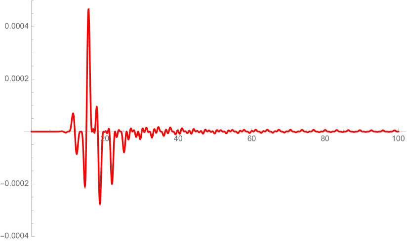
Figure 1. Plot of the function $J_{15}(r)J_{9}(r)J_{6}(r)J_{1}^{2}(r)J_{0}(r)r$ for $0\leq r\leq 100$.

Acknowledgements. The software Mathematica was heavily used in the brainstorming phase of the research project, as well as in the numerical part of the paper. We are thankful to Emanuel Carneiro for helpful discussions during the preparation of this work, and to Pavel Zorin-Kranich for pointing out an improvement to the first version of our Mathematica code. Finally, we would like to thank both the Hausdorff Center for Mathematics and the Hausdorff Institute for Mathematics for support.

2. Background on Bessel functions

We rewrite the definition (4) of the Bessel function in the form of a Bessel integral which is the starting point in [5, p. 338]. For $n\in\mathbb{Z}$ and $z\geq 0$, we claim that

(8) $$J_{n}(z)=\frac{1}{2\pi}\int_{-\pi}^{\pi}e^{iz\sin\theta}e^{-in\theta}d\theta.$$

More precisely, replacing $\theta=\omega+\pi/2$ in (8) and using even symmetry of the cosine we obtain for the right-hand side of (8):

(9) $$\frac{(-i)^{n}}{2\pi}\int_{-\pi}^{\pi}e^{iz\cos\omega}e^{-in\omega}d\omega=\frac{(-i)^{n}}{\pi}\int_{0}^{\pi}e^{iz\cos\omega}\cos(n\omega)d\omega,$$

from which the equivalence of (8) and (4) is evident.

The Bessel function, defined via (8) for general $z\in\mathbb{C}$, is an entire function. From (8) we obtain the estimate

(10) $$|J_{n}(z)|\leq e^{|\Im(z)|}.$$

Differentiation under the integral sign in (8) and integration by parts yield the following recurrence relations in the sense of meromorphic functions:

(11) $$J_{n-1}(z)-J_{n+1}(z) =2J_{n}^{\prime}(z),$$

(12) $$J_{n-1}(z)+J_{n+1}(z) =\frac{2n}{z}J_{n}(z).$$

A different representation of the Bessel function is the Poisson integral, which contains a power of a trigonometric function rather than a power of an exponential function:

(13) $${J}_{n}(z)=\frac{(z/2)^{n}}{\Gamma(n+1/2)\Gamma(1/2)}\int_{0}^{\pi}\cos(z\cos(\theta))\sin^{2n}(\theta)\,d\theta\ .$$

Here we use the Gamma function

$$\Gamma(s):=\int_{0}^{\infty}e^{-t}t^{s-1}dt\ ,$$

which satisfies the functional equation $s\Gamma(s)=\Gamma(s+1)$ and thus meromorphically extends the factorial, that is $\Gamma(n+1)=n!$ for natural numbers $n$. We mainly need the Gamma function for half-integer values, which can be expressed as

(14) $$\Gamma\Big{(}\frac{1}{2}+n\Big{)}=\frac{(2n)!}{4^{n}n!}\sqrt{\pi}\textrm{ and }\Gamma\Big{(}\frac{1}{2}-n\Big{)}=\frac{(-4)^{n}n!}{(2n)!}\sqrt{\pi}.$$

This can be recursively verified from $\Gamma(\frac{1}{2})=\sqrt{\pi}$, which in turn can be read from the well-known property

(15) $$\sin(\pi x)\Gamma(x)\Gamma(1-x)=\pi.$$

The latter can be seen by verifying periodicity of the left-hand side together with growth estimates which force the left-hand side to be constant.

To see equivalence of the Poisson integral representation (13) with (8), one verifies the case $n=0$ by substitution and then verifies by partial integration that the Poisson integral also satisfies the recursion relations (11) and (12). Combining these two second order recurrence relations into a first order relation between $J_{n}$ and $J_{n+1}$, equivalence of the two integral representations follows recursively by a uniqueness result for ordinary differential equations, where we use that both integral representations vanish for $z=0$ and $n>0$.

From the Poisson integral representation one sees the following estimate from [7, §3.31(1), p. 49], useful for small $z$:

(16) $$|J_{n}(z)|\leq\frac{|z|^{n}e^{|\Im{z}|}}{2^{n}n!}\ ,$$

where we have used

$$\frac{1}{n!}=\frac{1}{\Gamma(n+1/2)\Gamma(1/2)}\int_{0}^{\pi}\sin^{2n}(\theta)\,d\theta\ ,$$

which one proves by induction on $n$ using integration by parts.

We turn to the core integrals (7). The case $\ell=\pm 2$ will be the most pleasant to deal with via the following lemma:

Lemma 2.

Let $0\leq n,m$ have the same parity, and $1\leq k\leq n+m$. Then if $k$ is even

$$\int_{0}^{\infty}J_{n}(r)J_{m}(r)r^{-k}\cos(2r)\,dr=0\ ,$$

and if $k$ is odd

$$\int_{0}^{\infty}J_{n}(r)J_{m}(r)r^{-k}\sin(2r)\,dr=0\ .$$

Proof.

By the parity assumption, we may extend the integrals to the full real line. It then suffices to show that the Fourier transform

$$\int_{-\infty}^{\infty}J_{n}(r)J_{m}(r)r^{-k}e^{-i\xi r}\,dr$$

vanishes at $\xi=2$. Substituting $\xi=\cos\omega$ on the right-hand side of (9) yields

$$J_{n}(z)=\frac{(-i)^{n}}{\pi}\int_{-1}^{1}e^{iz\xi}\frac{\cos(n\arccos\xi)}{\sqrt{1-\xi^{2}}}d\xi\ .$$

Hence we see that $J_{n}$ is the Fourier transform of the function

$$B_{n}(\xi)=\frac{(-i)^{n}}{\pi}T_{n}(\xi)(1-\xi^{2})^{-1/2}1_{[-1,1]}(\xi)\ ,$$

where $T_{n}$ denotes the Chebysheff polynomial $T_{n}(\xi):=\cos(n\arccos\xi)$.

We first consider the case $k\leq n$ in the lemma. Then the Fourier transform $B_{n}^{(-k)}$ of $J_{n}(r)r^{-k}$ is still supported on $[-1,1]$ since $B_{n}$ has vanishing moments of orders $0,1,\ldots,k-1$. This can be deduced from (13). Seen as the convolution of an $L^{p^{\prime}}$ function with an $L^{p}$ function for $p=2^{-}$, the function $B_{n}^{(-k)}*B_{m}$ is continuous. Since it is also supported on the interval $[-2,2]$, it must vanish at $\xi=2$. This proves the lemma in case $k\leq n$. If $n<k\leq n+m$, we distribute some powers of $r$ over $J_{m}$ and argue similarly. ∎

The understanding of the dominant case $\ell=0$ of the core integrals (7) begins with Kapteyn’s identity, proved in a delightful two page paper [2].

Lemma 3 ([2]).

If $n,m\geq 0$ and $n+m\neq 0$, then

(17) $$\int_{0}^{\infty}J_{n}(r)J_{m}(r)r^{-1}dr=\frac{2}{\pi}\frac{\sin\frac{m-n}{2}\pi}{m^{2}-n^{2}}$$

with the following natural interpretation in case $n=m$:

$$\int_{0}^{\infty}J_{n}(r)^{2}r^{-1}dr=\frac{1}{2n}\ .$$

Note in particular that (17) vanishes if $m-n$ is a nonzero even integer. Moreover, identities (14), (15), and some algebra yield

$$\frac{2}{\pi}\frac{\sin\frac{m-n}{2}\pi}{m^{2}-n^{2}}=\frac{2^{-1}\Gamma(\frac{m+n}{2})}{\Gamma(\frac{m+n+2}{2})\Gamma(\frac{n-m+2}{2})\Gamma(\frac{m-n+2}{2})}.$$

From Kapteyn’s identity, one obtains the following more general result.

Lemma 4.

If $0\leq n,m$ and $1\leq k\leq n+m$, then

(18) $$\int_{0}^{\infty}J_{n}(r)J_{m}(r)r^{-k}dr=\frac{2^{-k}\Gamma(k)\Gamma(\frac{m+n+1-k}{2})}{\Gamma(\frac{m+n+1+k}{2})\Gamma(\frac{n-m+k+1}{2})\Gamma(\frac{m-n+k+1}{2})}\ .$$

Proof.

The identity is true for $k=1$ by Lemma 3. Let $k\geq 1$ be given and assume that identity (18) is true for this particular $k$. To prove the identity for $k+1$ we denote the integral in (18) by $\mathcal{I}_{n,m,k}$. Then, by the second recursion in (12) and using the induction hypothesis, we have that

$$\mathcal{I}_{n,m,k+1}=\frac{1}{2n}(\mathcal{I}_{n-1,m,k}+\mathcal{I}_{n+1,m,k})$$

$$=\frac{2^{-(k+1)}n^{-1}\Gamma(k)\Gamma(\frac{m+n-k}{2})}{\Gamma(\frac{m+n+k}{2})\Gamma(\frac{n-m+k}{2})\Gamma(\frac{m-n+k+2}{2})}+\frac{2^{-(k+1)}n^{-1}\Gamma(k)\Gamma(\frac{m+n+2-k}{2})}{\Gamma(\frac{m+n+2+k}{2})\Gamma(\frac{n-m+k+2}{2})\Gamma(\frac{m-n+k}{2})}=$$

$$\frac{2^{-(k+1)}\Gamma(k+1)\Gamma(\frac{m+n-k}{2})}{\Gamma(\frac{m+n+2+k}{2})\Gamma(\frac{n-m+k+2}{2})\Gamma(\frac{m-n+k+2}{2})}\frac{(m+n+k)(n-m+k)+(m+n-k)(m-n+k)}{4nk}$$

The second fraction in the last line is equal to $1$, and this proves the inductive step. ∎

Note in particular that if $k$ is odd and satisfies $k<|n-m|$, then (18) vanishes since the function $1/\Gamma$ has zeros at $s=0,-1,-2,\ldots$ Note also that three of the Gamma factors, the one with argument $k$ in the numerator and the two involving the difference $m-n$ in the denominator, typically form a binomial coefficient, which can be roughly estimated by $2^{k}$. An alternative approach to Lemma 4 is the integration theory of Weber and Schafheitlin as outlined in [7, §13.24, p. 398].

The case $\ell=\pm 4$ of the core integrals (7) gives small error terms which we estimate with the following lemma.

Lemma 5.

Let $0\leq n,m$ and $1\leq k<n+m$. Then:

$$\Big{|}\int_{0}^{\infty}J_{n}(r)J_{m}(r)r^{-k}e^{4ir}{dr}\Big{|}\leq\frac{2^{k-1}}{4^{n+m}}\frac{(n+m-k)!}{n!m!}.$$

Proof.

We estimate this integral by the descent method, changing the contour of integration to the contour consisting of a line segment from $0$ to $iN$ for some large $N$, then a line segment from $iN$ to $N$, and then a ray from $N$ to $\infty$ along the real axis. Only the first integral provides a substantial contribution, since the next two segments give contributions that tend to $0$ as $N$ tends to infinity.

Along the first segment of the contour the integral can be estimated using (16) by

$$\int_{0}^{\infty}|J_{n}(ix)||J_{m}(ix)|x^{-k}e^{-4x}{dx} \leq\frac{1}{n!m!}\frac{1}{2^{n+m}}\int_{0}^{\infty}x^{n+m-k}e^{-2x}{dx}$$

$$=\frac{2^{k-1}}{4^{n+m}}\frac{(n+m-k)!}{n!m!}.$$

The integral over the second part of the contour is estimated using (10) by

$$\sqrt{2}\int_{0}^{N}|J_{n}(x+i(N-x))||J_{m}(x+i(N-x))||x+i(N-x)|^{-k}e^{-4(N-x)}{dx}$$

$$\leq\sqrt{2}\int_{0}^{N}(N/\sqrt{2})^{-k}e^{-2(N-x)}{dx}\leq 2^{k+1}N^{-k}\ ,$$

which tends to 0 as $N\rightarrow\infty$. The integral over the third piece of the contour is estimated using the fact that the functions $J_{n}$ and $J_{m}$ are in $L^{4}$ as Fourier transforms of $L^{4/3}$ functions and thus the continuous function $J_{n}(r)J_{m}(r)r^{-1}$ is in $L^{1}$. It then follows from the dominated convergence theorem that

$$\lim_{N\to\infty}\int_{N}^{\infty}|J_{n}(r)J_{n+m}(r)|r^{-1}{dr}=0\ .$$

Adding the contour integrals and letting $N\to\infty$ yields the desired bound. ∎

To arrive at the core integrals, we need asymptotic expansions of the Bessel functions near infinity as in the following lemma.

Lemma 6.

Let $n\in\mathbb{N}$ and $\Re(z)>0$. Let $\omega_{n}=z-{n\pi}/{2}-{\pi}/{4}$. Let $\ell\in\mathbb{N}$ be such that $\ell\geq\max\{n-1/2,1\}$. If $\ell$ is even, then

(19) $$J_{n}(z)=\Big{(}\frac{2}{\pi z}\Big{)}^{\frac{1}{2}}\Big{[}(\cos\omega_{n})\left(\sum_{k=0}^{\frac{\ell}{2}-1}(-1)^{k}\frac{a_{2k}(n)}{z^{2k}}\right)-(\sin\omega_{n})\left(\sum_{k=0}^{\frac{\ell}{2}-1}(-1)^{k}\frac{a_{2k+1}(n)}{z^{2k+1}}\right)\Big{]}+R_{n,\ell}(z).$$

If $\ell$ is odd, then

(20) $$J_{n}(z)=\Big{(}\frac{2}{\pi z}\Big{)}^{\frac{1}{2}}\Big{[}(\cos\omega_{n})\left(\sum_{k=0}^{\frac{\ell-1}{2}}(-1)^{k}\frac{a_{2k}(n)}{z^{2k}}\right)-(\sin\omega_{n})\left(\sum_{k=0}^{\frac{\ell-3}{2}}(-1)^{k}\frac{a_{2k+1}(n)}{z^{2k+1}}\right)\Big{]}+{R}_{n,\ell}(z).$$

Here the coefficients $a_{j}(n)$ are defined by

(21) $$a_{j}(n)=\frac{\Gamma(n+j+\frac{1}{2})}{\Gamma(n-j+\frac{1}{2})j!2^{j}},$$

and the remainder function ${R}_{n,\ell}$ satisfies the bounds

$$|R_{n,\ell}(z)|\leq\Big{(}\frac{2}{\pi|z|}\Big{)}^{\frac{1}{2}}\frac{\Gamma(n+\ell+\frac{1}{2})}{|\Gamma(n-\ell+\frac{1}{2})|\ell!}\left(\frac{|z|}{\Re(z)}\right)^{\ell-n+\frac{1}{2}}\cosh(\Im(z))\left(\frac{1}{2|z|}\right)^{\ell}.$$

Proof.

We expand on the proof outlined in Watson [7, §7.3, p. 205]. The change of variables $t=\cos\theta$ turns the Poisson integral (13) into

$${J}_{n}(z)=\frac{(z/2)^{n}}{\Gamma(n+1/2)\Gamma(1/2)}\int_{-1}^{1}\cos(zt)(1-t^{2})^{n-1/2}\,dt\ .$$

We split

$$J_{n}(z)=\frac{1}{2}(J_{n}^{+}(z)+J_{n}^{-}(z)),$$

with

$${J}_{n}^{+}(z)=\frac{(z/2)^{n}}{\Gamma(n+1/2)\Gamma(1/2)}\int_{-1}^{1}e^{izt}(1-t^{2})^{n-1/2}\,dt$$

and $J_{n}^{-}(\overline{z})=\overline{J_{n}^{+}({z})}$. Now we change the contour in the integral for $J_{n}^{+}$ towards a $\Pi$-shaped contour consisting of the line segment from $-1$ to $-1+iN$, followed by the line segment from $-1+iN$ to $1+iN$, and then the line segment from $1+iN$ to $1$. On that contour as well as on its convex hull, we have $\Re(1-t^{2})\geq 0$ with equality only at the end points of the contour. Hence we may choose the continuous branch of the square root function on the slit plane $\mathbb{C}\setminus(-\infty,0)$ which takes positive values on the positive real axis. For simplicity of notation, let us introduce the half-integer $\nu:=n-1/2$. The integral over the first segment of the contour becomes

$$\frac{(z/2)^{\nu+1/2}}{\Gamma(\nu+1)\Gamma(1/2)}\int_{0}^{N}e^{-iz}e^{-zs}(2is+s^{2})^{\nu}i\,ds =\frac{e^{-iz}}{(2\pi z)^{1/2}\Gamma(\nu+1)}\int_{0}^{zN}e^{-u}u^{\nu}(i+\frac{u}{2z})^{\nu}i\,du$$

$$=\frac{e^{i(-z+(\nu+1)\pi/2)}}{(2\pi z)^{1/2}\Gamma(\nu+1)}\int_{0}^{zN}e^{-u}u^{\nu}(1-\frac{iu}{2z})^{\nu}\,du\ ,$$

where in the first identity we replaced $zs$ by $u$ and rotated the contour towards the line segments from $0$ to $zN$, and used $\Gamma(1/2)=\pi^{1/2}$. In the second identity, we first pulled an integer power of $i$ out of the integral and and then pulled half a power of $i$ out of the integral without leaving the domain of definition of the chosen branch of the square root function. If $\Re(z)>0$, then this last integral has a limit as $N\to\infty$. Similarly, the integral over the third line segment becomes

$$-\frac{(z/2)^{\nu+1/2}}{\Gamma(\nu+1)\Gamma(1/2)}\int_{0}^{N}e^{iz}e^{-zs}(-2is+s^{2})^{\nu}i\,ds=\frac{e^{i(z-(\nu+1)\pi/2}}{(2\pi z)^{1/2}\Gamma(\nu+1)}\int_{0}^{zN}e^{-u}u^{\nu}(1+\frac{iu}{2z})^{\nu}\,du\ .$$

If $\Re(z)>0$, then the limit again exists. Moreover, the integral over the second line segment tends to $0$ as $N\to\infty$. We therefore obtain

$$J_{n}^{+}(z)=\frac{(2\pi z)^{-1/2}}{\Gamma(\nu+1)}\int_{0}^{\infty}e^{-u}u^{\nu}\left[e^{-i\omega_{n}}(1-\frac{iu}{2z})^{\nu}+e^{i\omega_{n}}(1+\frac{iu}{2z})^{\nu}\right]\,du\ ,$$

where $\omega_{n}=z-{n\pi}/{2}-{\pi}/{4}=z-(\nu+1)\pi/2$, and the contour has been changed to one along the real axis.

The function $(1+\alpha u)^{\nu}$ is infinitely differentiable in $u\in[0,\infty)$ for any $\alpha\in\mathbb{C}\setminus(-\infty,0]$. Taylor’s expansion gives, for any $\ell\geq 1$,

$$(1+\alpha u)^{\nu}=\sum_{k=0}^{\ell-1}\frac{\Gamma(\nu+1)}{\Gamma(\nu+1-k)}\frac{\left(\alpha u\right)^{k}}{k!}+r\frac{u^{\ell}}{\ell!},$$

where $r$ is the $\ell$-th derivative of the function $u\mapsto(1+\alpha u)^{\nu}$ at some point $u_{0}\in[0,u]$. If $\ell>\nu$, then this derivative is proportional to a negative power of the function and thus attains its maximum at the point where the value of the function comes closest to the origin. This point equals $u=-\Re(\alpha)/|\alpha|^{2}$ and the value of the $\ell$-th derivative there equals

$$\frac{\Gamma(\nu+1)}{\Gamma(\nu+1-\ell)}\alpha^{\ell}\Big{(}1-\frac{\Re(\alpha)}{\overline{\alpha}}\Big{)}^{\nu-\ell}\ .$$

Hence we can write for the remainder term

$$r\frac{u^{\ell}}{\ell!}=\theta(u)\frac{\Gamma(\nu+1)}{\Gamma(\nu+1-\ell)}\left|1-\frac{\Re(\alpha)}{\overline{\alpha}}\right|^{\nu-\ell}\frac{\left(\alpha u\right)^{\ell}}{\ell!}$$

for some $|\theta(u)|\leq 1$ that also depends on $\alpha$. Note that

$$|1-\frac{\Re(\alpha)}{\overline{\alpha}}|=\frac{|\overline{\alpha}-\Re(\alpha)|}{|\alpha|}=\frac{|\Im(\alpha)|}{|\alpha|},$$

and the latter equals $\Re(z)/|z|$ if $\alpha=\pm i/(2z)=\pm i\overline{z}/(2|z|^{2})$. For $\Re(z)>0$, we have that $1\pm\frac{iu}{2z}$ is not real, hence we may insert the Taylor expansion into the integral for $J_{n}^{+}$, and obtain for $J_{n}^{+}(z)$ the expression

$$(2\pi z)^{-1/2}\sum_{k=0}^{\ell-1}\frac{1}{\Gamma(\nu+1-k)k!}\int_{0}^{\infty}e^{-u}u^{\nu+k}\left[e^{-i\omega_{n}}\left(\frac{-i}{2z}\right)^{k}+e^{i\omega_{n}}\left(\frac{i}{2z}\right)^{k}\right]\,du+R(z)$$

$$=(2\pi z)^{-1/2}\sum_{k=0}^{\ell-1}\frac{\Gamma(\nu+k+1)}{\Gamma(\nu+1-k)k!}\left[e^{-i\omega_{n}}\left(\frac{-i}{2z}\right)^{k}+e^{i\omega_{n}}\left(\frac{i}{2z}\right)^{k}\right]+R(z)\ ,$$

where the remainder term $R=R_{n,\ell}$ satisfies

$$|R_{n,\ell}(z)|\leq\Big{(}\frac{2}{\pi|z|}\Big{)}^{1/2}\frac{\Gamma(\nu+\ell+1)}{|\Gamma(\nu+1-\ell)|\ell!}\left(\frac{|z|}{\Re(z)}\right)^{\ell-\nu}\cosh(\Im(z))\left(\frac{1}{2|z|}\right)^{\ell}\ .$$

We split the summation into even integers and odd integers to obtain

$$J_{n}^{+}(z) =\Big{(}\frac{2}{\pi z}\Big{)}^{1/2}\sum_{\begin{subarray}{c}0\leq k<\ell:\\ k\ \rm even\end{subarray}}(-1)^{k/2}\frac{\Gamma(\nu+k+1)}{\Gamma(\nu+1-k)k!2^{k}}\cos(\omega_{n})\left(\frac{1}{z}\right)^{k}$$

$$-\Big{(}\frac{2}{\pi z}\Big{)}^{1/2}\sum_{\begin{subarray}{c}0\leq k<\ell:\\ k\ \rm odd\end{subarray}}(-1)^{(k-1)/2}\frac{\Gamma(\nu+k+1)}{\Gamma(\nu+1-k)k!2^{k}}\sin(\omega_{n})\left(\frac{1}{z}\right)^{k}+R_{n,\ell}(z).$$

This completes the proof of the lemma. ∎

We specify our findings into explicit first order asymptotics valid for sufficiently large $z$ near the positive real axis. We have with the notation from the above proof:

Corollary 7.

Let $z\in\mathbb{C}$ be such that $\Im(z)<\Re(z)$. Then

$$\left|J_{0}^{\pm}(z)-\left(\frac{2}{\pi z}\right)^{1/2}\cos(\omega_{0})\right|\leq\frac{1}{8|z|}\left(\frac{2}{\pi|z|}\right)^{1/2}\cosh(\Im(z))\left(\frac{|z|}{|\Re(z)|}\right)^{3/2}\ ,$$

$$\left|J_{1}^{\pm}(z)-\left(\frac{2}{\pi z}\right)^{1/2}\cos(\omega_{1})\right|\leq\frac{3}{8|z|}\left(\frac{2}{\pi|z|}\right)^{1/2}\cosh(\Im(z))\left(\frac{|z|}{|\Re(z)|}\right)^{1/2}\ ,$$

and if $n>1$ and $\Re(z)>n^{2}$, then

$$\left|J_{n}^{\pm}(z)-\left(\frac{2}{\pi z}\right)^{1/2}\cos(\omega_{n})\right|\leq\left(\frac{2}{\pi|z|}\right)^{1/2}\frac{n^{2}}{|z|}\cosh(\Im(z))\left(\frac{|z|}{|\Re(z)|}\right)^{1/2}\ .$$

Proof.

Following the previous argument, only the last inequality requires explanation. We choose $\ell=n=\nu+1/2$, and apply the above expansion with the observation that

$$\frac{\Gamma(\nu+1+k)}{\Gamma(\nu+1-k)}\leq\Big{(}\nu+\frac{1}{2}\Big{)}^{2k}$$

for $k\leq\nu$. It follows that

$$\left|J_{n}^{\pm}(z)-\left(\frac{2}{\pi z}\right)^{1/2}\cos(\omega_{n})\right|\leq\left(\frac{2}{\pi|z|}\right)^{1/2}\sum_{k=1}^{\ell-1}n^{2k}\cosh(\Im(z))(2|z|)^{-k}+R$$

$$\leq\left(\frac{2}{\pi|z|}\right)^{1/2}\cosh(\Im(z))\frac{n^{2}}{|z|}(1-2^{1-\ell})+R\leq\left(\frac{2}{\pi|z|}\right)^{1/2}\cosh(\Im(z))\frac{n^{2}}{|z|}\left(\frac{|z|}{|\Re(z)|}\right)^{1/2},$$

where in the last line we estimated the remainder similarly to the terms in the expansion. ∎

One proves explicit asymptotics with one extra term in a similar way:

Corollary 8.

Let $z\in\mathbb{C}$ be such that $\Re(z)>1/4$ and $\Im(z)<\Re(z)$. Then

$$\left|J_{0}^{\pm}(z)-\left(\frac{2}{\pi z}\right)^{1/2}\cos(\omega_{0})+\frac{1}{8z}\left(\frac{2}{\pi z}\right)^{1/2}\sin(\omega_{0})\right|\leq\\ \leq\frac{9}{128|z|^{2}}\left(\frac{2}{\pi|z|}\right)^{1/2}\cosh(|\Im(z)|)\left(\frac{|z|}{|\Re(z)|}\right)^{5/2},$$

$$\left|J_{1}^{\pm}(z)-\left(\frac{2}{\pi z}\right)^{1/2}\cos(\omega_{1})+\frac{3}{8z}\left(\frac{2}{\pi z}\right)^{1/2}\sin(\omega_{1})\right|\leq\\ \leq\frac{15}{128|z|^{2}}\left(\frac{2}{\pi|z|}\right)^{1/2}\cosh(\Im(z))\left(\frac{|z|}{|\Re(z)|}\right)^{3/2},$$

and if $n>1$ and $\Re(z)>n^{2}$, then

$$\left|J_{n}^{\pm}(z)-\left(\frac{2}{\pi z}\right)^{1/2}\cos(\omega_{n})+\frac{4n^{2}-1}{8z}\left(\frac{2}{\pi z}\right)^{1/2}\sin(\omega_{n})\right|\leq\\ \leq\frac{1}{4}\left(\frac{2}{\pi|z|}\right)^{1/2}\cosh(\Im(z))\frac{n^{4}}{|z|^{2}}\left(\frac{|z|}{|\Re(z)|}\right)^{1/2}.$$

Finally, we need zero order upper bounds for the asymptotic expansion:

Corollary 9.

For $r>0$, we have that

• $$|J_{0}(r)|\leq\frac{9}{8}\left(\frac{2}{\pi r}\right)^{1/2},$$

• $$|J_{1}(r)|\leq\frac{11}{8}\left(\frac{2}{\pi r}\right)^{1/2}.$$

Proof.

This follows for $r>1$ from Corollary 7, while for $r\leq 1$ it follows from the trivial bound $|J_{n}|\leq 1$. ∎

Remark. Using more refined oscillatory techniques related to Sturm’s comparision principle, the sharper bound $r^{1/2}|J_{0}(r)|\leq\left(2/{\pi}\right)^{1/2}$ is established in [3]. However, the bounds given by Corollary 9 suffice for our purpose, and its proof is more in light with the elementary nature of the present paper.

3. Useful estimates involving the Gamma function

A version [4] of Stirling’s formula for the Gamma function states that, for $x\geq 0$,

(22) $$\Gamma(x)=\sqrt{2\pi}x^{x-1/2}e^{-x}e^{\mu(x)},$$

where the function $\mu$ satisfies the double inequality

(23) $$\frac{1}{12x+1}<\mu(x)<\frac{1}{12x}.$$

The starting point for all the convex estimates we need is the following well-known result:

Lemma 10.

For $x>0$, the function $x\mapsto\log(\Gamma(x))$ is convex.

Proof.

Let $x,y>0$ and $0<\lambda<1$. Set $p=\frac{1}{\lambda}$ and $q=\frac{1}{1-\lambda}$. It suffices to show that

(24) $$\Gamma\Big{(}\frac{x}{p}+\frac{y}{q}\Big{)}\leq\Gamma(x)^{\frac{1}{p}}\Gamma(y)^{\frac{1}{q}},$$

for then the result follows by taking logarithms on both sides. To verify (24), consider the auxiliary functions

$$f(t):=t^{\frac{x-1}{p}}e^{-\frac{t}{p}}\textrm{ and }g(t):=t^{\frac{y-1}{q}}e^{-\frac{t}{q}},$$

which satisfy

$$f(t)g(t)=t^{\frac{x}{p}+\frac{y}{q}-1}e^{-t},\;\;\;f(t)^{p}=t^{x-1}e^{-t},\textrm{ and }g(t)^{q}=t^{y-1}e^{-t}.$$

The result is thus a consequence of Hölder’s inequality. ∎

Corollary 11.

Let $x\geq\frac{1}{2}$. Then:

$$\sqrt{x-1/2}\leq\frac{\Gamma\Big{(}x+\frac{1}{2}\Big{)}}{\Gamma(x)}\leq\sqrt{x}.$$

Proof.

Use the identity $x=\Gamma(x+1)/\Gamma(x)$ together with log convexity of $\Gamma$. ∎

Corollary 12.

Let $x\geq y>0$ and $w\geq 0$. Then:

$$\frac{\Gamma(x)}{\Gamma(y)}\leq\frac{\Gamma(x+w)}{\Gamma(y+w)}.$$

Proof.

For fixed $w\geq 0$, we claim that the function

$$x\mapsto\frac{\Gamma(x)}{\Gamma(x+w)}$$

is decreasing in $x$. This happens if the inequality

$$\frac{\Gamma^{\prime}(x)}{\Gamma(x)}\leq\frac{\Gamma^{\prime}(x+w)}{\Gamma(x+w)}$$

holds for every $x>0$, which in turn is a consequence of the log convexity of $\Gamma$ proved in Lemma 10. ∎

The following lemma estimates binomial coefficients.

Lemma 13.

Let $x\geq 1$ and let $0\leq d<x$ be an integer. Then:

(25) $$\frac{\Gamma(2x)}{\Gamma(x-d)\Gamma(x+d)}\leq\frac{e^{1/24}}{2\sqrt{\pi}}x^{1/2}2^{2x}e^{-d^{2}/x}.$$

Proof.

By Stirling’s formula (22), we have that

$$\frac{\Gamma(2x)}{\Gamma(x)^{2}}=\frac{(2x)^{2x-1/2}}{\sqrt{2\pi}x^{2x-1}}e^{\mu(2x)-2\mu(x)}=\frac{x^{1/2}2^{2x}}{2\sqrt{\pi}}e^{\mu(2x)-2\mu(x)}.$$

Also, since $x\geq 1$, we have that $\mu(2x)\leq\frac{1}{24}$, and therefore

$$e^{\mu(2x)-2\mu(x)}\leq e^{\mu(2x)}\leq e^{1/24}.$$

It follows that

$$\frac{\Gamma(2x)}{\Gamma(x)^{2}}\leq\frac{e^{1/24}}{2\sqrt{\pi}}x^{1/2}2^{2x}.$$

By induction, observe that

$$\frac{\Gamma(x)\Gamma(x+1)}{\Gamma(x-d)\Gamma(x+d+1)}=\prod_{j=1}^{d}\frac{x-j}{x+j}\leq\prod_{j=1}^{d}e^{-2j/x}=e^{-(d^{2}+d)/x},$$

whenever $d$ is an integer satisfying $0\leq d<x$. This is a consequence of the elementary inequality

$$\frac{1-y}{1+y}\leq e^{-2y},$$

which is valid in particular for $y\in[0,1]$. Using $(x+d)/d\leq e^{d/x}$ we obtain that

$$\frac{\Gamma(x)\Gamma(x)}{\Gamma(x-d)\Gamma(x+d)}\leq e^{d/x}\prod_{j=1}^{d}\frac{x-j}{x+j}\leq e^{d/x}\prod_{j=1}^{d}e^{-2j/x}=e^{-d^{2}/x},$$

again for integers $d\in[0,x)$. Finally,

$$\frac{\Gamma(2x)}{\Gamma(x-d)\Gamma(x+d)}=\frac{\Gamma(2x)}{\Gamma(x)^{2}}\frac{\Gamma(x)\Gamma(x)}{\Gamma(x-d)\Gamma(x+d)}\leq\frac{e^{1/24}}{2\sqrt{\pi}}x^{1/2}2^{2x}e^{-d^{2}/x},$$

as desired. ∎

Remark. The inequality

$$\frac{\Gamma(x)\Gamma(x)}{\Gamma(x-d)\Gamma(x+d)}\leq e^{-d^{2}/x},$$

is still valid for non-integer values of $d\in[0,x)$, and therefore Lemma 13 holds in this case as well.

We will also need estimates for the magnitude of the coefficients $a_{j}(m)$ defined in (21) when $j$ is close to $m$. More precisely, in Section 5 we will need good upper bounds for the quantities $|a_{m+4}(m)|.$ For small values of $m$, we compute them explicitly. For large values of $m$, we estimate these quantities via the following lemma.

Lemma 14.

For any natural number $m\geq 1$, we have that

$$|a_{m+4}(m)|\leq\frac{105}{16}\sqrt{\frac{2}{\pi}}(2m-1)^{-1/2}2^{m}m^{m}e^{-m}.$$

Proof.

The goal is to bound the absolute value of

$$a_{m+4}(m)=\frac{\Gamma(2m+9/2)}{\Gamma(-7/2)\Gamma(m+5)2^{m+4}}.$$

Making repeated use of the identity $\Gamma(x+1)=x\Gamma(x)$, together with the convexity estimate from Corollary 11 and Stirling’s formula (22), we have that

$$|a_{m+4}(m)| \leq 2^{5}\frac{\Gamma(2m-1/2)}{\Gamma(-7/2)\Gamma(m)2^{m+4}}$$

$$\leq 2(2m-1)^{-1/2}\frac{\Gamma(2m)}{\Gamma(-7/2)\Gamma(m)2^{m}}$$

$$=\frac{2(2m-1)^{-1/2}}{\Gamma(-7/2)2^{m}}\frac{(2m)^{2m-1/2}}{m^{m-1/2}}e^{-m}e^{\mu(2m)-\mu(m)}.$$

The bounds (23) for the function $\mu$ imply that $\mu(2m)\leq\mu(m)$, and so $e^{\mu(2m)-\mu(m)}\leq 1$. It follows that

(26) $$|a_{m+4}(m)|\leq\frac{2(2m-1)^{-1/2}}{\Gamma(-7/2)2^{m}}2^{2m-1/2}m^{m}e^{-m}.$$

The value $\Gamma(-7/2)=\frac{16\sqrt{\pi}}{105}$ can be computed via the second formula in (14), and this completes the proof. ∎

4. Part I. Expanding $J_{0}$ and $J_{1}$

In the next four sections, we will be working under the standing assumption that $n\geq n_{0}:=20$. We start by asymptotically expanding the Bessel functions of order 0 and 1 and their relevant products. Due to need of accuracy, we must consider asymptotic expansions of length six and keep track of all the terms. The following notation will be convenient. Let us say that

$$a\sim(a_{0})+(a_{1})+(a_{2})+(a_{3})+(a_{4})+(a_{5}){\rm\ with\ remainders\ }r_{0},r_{1},r_{2},r_{3},r_{4},r_{5},r_{6}$$

if

$$\Big{|}a-\sum_{i=1}^{k}a_{i-1}\Big{|}\leq r_{k},\textrm{ for every }0\leq k\leq 6.$$

We also call $r_{6}$ the last remainder. Suppose additionally that

$$b\sim(b_{0})+(b_{1})+(b_{2})+(b_{3})+(b_{4})+(b_{5}){\rm\ with\ remainders\ }s_{0},s_{1},s_{2},s_{3},s_{4},s_{5},s_{6}.$$

Then we have the following product formula:

$$ab\sim\sum_{k=0}^{5}(\sum_{i=0}^{k}a_{i}b_{k-i})$$

with remainders

$$r_{0}s_{k}+\sum_{i=1}^{k}r_{i}|b_{k-i}|,\textrm{ for every }0\leq k\leq 6.$$

Recall the coefficients $a_{0}(n)$ through $a_{5}(n)$ for $n=0$,

$$1,\ -\frac{1}{8},\ \frac{9}{128},\ -\frac{75}{1024},\ \frac{3675}{32768},\ -\frac{59535}{262144},\ \frac{2401245}{4194304},\ -\frac{57972915}{33554432},$$

and for $n=1$,

$$1,\ \frac{3}{8},\ -\frac{15}{128},\ \frac{105}{1024},\ -\frac{4725}{32768},\ \frac{72765}{262144},\ -\frac{2837835}{4194304},\ \frac{66891825}{33554432}.$$

To make the forthcoming notation less cumbersome, let us define, in view of Lemma 6,

$$\mathfrak{J}_{n}(r):=\left(\frac{\pi r}{2}\right)^{1/2}J_{n}(r).$$

To avoid writing many fractions, we further define $t:=(16r)^{-1}$. We also set

$$\mathfrak{c}:=\cos(r-\pi/4)\textrm{ and }\mathfrak{s}:=\sin(r-\pi/4).$$

From Lemma 6 and Corollary 9, we have that

$$\mathfrak{J}_{0}(r)\sim(\mathfrak{c})+(2t\mathfrak{s})+(-18t^{2}\mathfrak{c})+(-300t^{3}\mathfrak{s})+(7350t^{4}\mathfrak{c})+(238140t^{5}\mathfrak{s})$$

with remainders discussed there as

$$\frac{9}{8},\ 2t,\ 18t^{2},\ 300t^{3},\ 7350t^{4},\ 238140t^{5},\ 9604980t^{6}.$$

In a similar way,

$$\mathfrak{J}_{1}(r)\sim(\mathfrak{s})+(6t\mathfrak{c})+(30t^{2}\mathfrak{s})+(-420t^{3}\mathfrak{c})+(-9450t^{4}\mathfrak{s})+(291060t^{5}\mathfrak{c})$$

with remainders

$$\frac{11}{8},\ 6t,\ 30t^{2},\ 420t^{3},\ 9450t^{4},\ 291060t^{5},\ 11351340t^{6}.$$

Applying the product formula, we obtain successively

$$\mathfrak{J}_{0}^{2}(r)\sim(\mathfrak{c}^{2})+(4t\mathfrak{c}\mathfrak{s})+(-36t^{2}\mathfrak{c}^{2}+4t^{2}\mathfrak{s}^{2})+(-672t^{3}\mathfrak{c}\mathfrak{s})+\\ +(15024t^{4}\mathfrak{c}^{2}-1200t^{4}\mathfrak{s}^{2})+(516480t^{5}\mathfrak{c}\mathfrak{s})$$

with remainders

$$\frac{81}{64},\ \frac{17}{4}t,\ \frac{169}{4}t^{2},\ \frac{1419}{2}t^{3},\ \frac{68571}{4}t^{4},\ \frac{1092495}{2}t^{5},\ \frac{43435485}{2}t^{6},$$

and

(27) $$\mathfrak{J}_{0}^{3}(r)\sim\mathfrak{J}_{000}(r):= (\mathfrak{c}^{3})+(6t\mathfrak{c}^{2}\mathfrak{s})+(-54t^{2}\mathfrak{c}^{3}+12t^{2}\mathfrak{c}\mathfrak{s}^{2})+(-1116t^{3}\mathfrak{c}^{2}\mathfrak{s}+8t^{3}\mathfrak{s}^{3})$$

$$+(23022t^{4}\mathfrak{c}^{3}-3816t^{4}\mathfrak{c}\mathfrak{s}^{2})+(836964t^{5}\mathfrak{c}^{2}\mathfrak{s}-3600t^{5}\mathfrak{s}^{3})$$

with remainders

$$\frac{729}{512},\ \frac{217}{32}t,\ \frac{2353}{32}t^{2},\ \frac{20003}{16}t^{3},\ \frac{956787}{32}t^{4},\ \frac{15017799}{16}t^{5},\ \frac{588969477}{16}t^{6}.$$

In particular,

(28) $$|\mathfrak{J}_{0}^{3}(r)-\mathfrak{J}_{000}(r)|\leq\frac{588969477}{16}(16r)^{-6}.$$

On the other hand, we have

$$\mathfrak{J}_{1}^{2}(r)\sim(\mathfrak{s}^{2})+(12t\mathfrak{c}\mathfrak{s})+(36t^{2}\mathfrak{c}^{2}+60t^{2}\mathfrak{s}^{2})+(-480t^{3}\mathfrak{c}\mathfrak{s})+\\ +(-5040t^{4}\mathfrak{c}^{2}-18000t^{4}\mathfrak{s}^{2})+(443520t^{5}\mathfrak{c}\mathfrak{s})$$

with remainders

$$\frac{121}{64},\ \frac{57}{4}t,\ \frac{429}{4}t^{2},\ \frac{2715}{2}t^{3},\ \frac{113535}{4}t^{4},\ \frac{1659735}{2}t^{5},\ \frac{62391105}{2}t^{6},$$

and

(29) $$(\mathfrak{J}_{1}^{2}\mathfrak{J}_{0})(r)\sim\mathfrak{J}_{110}(r):= (\mathfrak{c}\mathfrak{s}^{2})+(12t\mathfrak{c}^{2}\mathfrak{s}+2t\mathfrak{s}^{3})+(36t^{2}\mathfrak{c}^{3}+66t^{2}\mathfrak{c}\mathfrak{s}^{2})+(-624t^{3}\mathfrak{c}^{2}\mathfrak{s}-180t^{3}\mathfrak{s}^{3})$$

$$+(-5688t^{4}\mathfrak{c}^{3}-16290t^{4}\mathfrak{c}\mathfrak{s}^{2})+(519480t^{5}\mathfrak{c}^{2}\mathfrak{s}+184140t^{5}\mathfrak{s}^{3})$$

with remainders

$$\frac{1089}{512},\ \frac{577}{32}t,\ \frac{5433}{32}t^{2},\ \frac{38331}{16}t^{3},\ \frac{1638411}{32}t^{4},\ \frac{23971455}{16}t^{5},\ \frac{897834285}{16}t^{6}.$$

In particular,

(30) $$|(\mathfrak{J}_{1}^{2}\mathfrak{J}_{0})(r)-\mathfrak{J}_{110}(r)|\leq\frac{897834285}{16}(16r)^{-6}.$$

Inequalities (28) and (30) are at the core of the following result, the proof of which does not require $m$ to be even, nor $m\leq n$.

Estimate A. For $n\geq n_{0}=20$ and $m\geq 0$, we have

(31) $$\Big{|}\int_{0}^{\infty}J_{n+m}J_{n}\mathfrak{J}_{m}(\mathfrak{J}_{0}^{3}-\mathfrak{J}_{000})r^{-1}dr\Big{|}\leq 0.74n_{0}^{-1/2}(n+m)^{-6},$$

(32) $$\Big{|}\int_{0}^{\infty}J_{n+m}J_{n}\mathfrak{J}_{m}(\mathfrak{J}_{1}^{2}\mathfrak{J}_{0}-\mathfrak{J}_{110})r^{-1}dr\Big{|}\leq 1.12n_{0}^{-1/2}(n+m)^{-6}.$$

Proof of Estimate A.

Using the Cauchy-Schwarz inequality and Lemmata 3 and 4 to compute the integrals, we have that

$$\int_{0}^{\infty}|J_{n}J_{n+m}\mathfrak{J}_{m}|r^{-7}{dr} \leq\Big{(}\frac{\pi}{2}\Big{)}^{1/2}\Big{(}\int_{0}^{\infty}J_{n}^{2}\frac{dr}{r}\Big{)}^{1/2}\Big{(}\int_{0}^{\infty}J_{n+m}^{2}\frac{dr}{r^{12}}\Big{)}^{1/2}$$

$$=\Big{(}\frac{1}{2n}\Big{)}^{1/2}\Big{(}\frac{128}{693}\frac{\Gamma(n+m-\frac{11}{2})}{\Gamma(n+m+\frac{13}{2})}\Big{)}^{1/2}$$

$$\leq a_{0}^{1/2}\Big{(}\frac{64}{693n}\Big{)}^{1/2}(n+m)^{-6},$$

where

$$a_{0}:=\sup_{\ell\geq n_{0}}\frac{\Gamma(\ell-\frac{11}{2})}{\Gamma(\ell+\frac{13}{2})}\ell^{12}=\frac{\Gamma(\frac{29}{2})}{\Gamma(\frac{53}{2})}20^{12}\leq 1.21.$$

Thus, for $n\geq n_{0}$, the left-hand side of inequality (31) is bounded by

$$\leq\frac{588969477/16}{16^{6}}a_{0}^{1/2}\Big{(}\frac{64}{693n}\Big{)}^{1/2}(n+m)^{-6}\leq\alpha n_{0}^{-1/2}(n+m)^{-6},$$

where

$$\alpha=\frac{588969477/16}{16^{6}}a_{0}^{1/2}\Big{(}\frac{64}{693}\Big{)}^{1/2}\leq 0.74.$$

In a similar way, for $n\geq n_{0}$, the left-hand side of inequality (32) is bounded by

$$\leq\frac{897834285/16}{16^{6}}a_{0}^{1/2}\Big{(}\frac{64}{693n}\Big{)}^{1/2}(n+m)^{-6}\leq\beta n_{0}^{-1/2}(n+m)^{-6},$$

where

$$\beta=\frac{897834285/16}{16^{6}}a_{0}^{1/2}\Big{(}\frac{64}{693}\Big{)}^{1/2}\leq 1.12.$$

∎

5. Part II. Expanding $J_{m}$

Start by noting that $\cos\omega_{m}=(-1)^{m/2}\mathfrak{c}$ and $\sin\omega_{m}=(-1)^{m/2}\mathfrak{s}$ since $m$ is an even integer. We have that

(33) $$\mathfrak{J}_{m}(r)-\rho_{m}(r)=(-1)^{m/2}\Big{(}\mathfrak{c}\sum_{k=0}^{\frac{m}{2}+1}(-1)^{k}(16t)^{2k}a_{2k}(m)-\mathfrak{s}\sum_{k=0}^{\frac{m}{2}+1}(-1)^{k}(16t)^{2k+1}a_{2k+1}(m)\Big{)},$$

where the error term $\rho_{m}$ is implicitly defined by this identity. From Lemma 6 we know that

(34) $$|\rho_{m}(r)|\leq\frac{|a_{m+4}(m)|}{r^{m+4}}$$

for every $r\geq 0$. The main integrals, which are the subject of the next section, arise from replacing $\mathfrak{J}_{m}\mathfrak{J}_{000}$ by

(35) $$\mathfrak{J}_{m000}:=(\mathfrak{J}_{m}-\rho_{m})\mathfrak{J}_{000},$$

and $\mathfrak{J}_{m}\mathfrak{J}_{110}$ by

(36) $$\mathfrak{J}_{m110}:=(\mathfrak{J}_{m}-\rho_{m})\mathfrak{J}_{110}.$$

Estimating the error term in this replacement is the main goal of the present section. We formulate it as

Estimate B. Let $n\geq n_{0}=20$ and $m$ be even.

If $m=0$, then

(37) $$\Big{|}\int_{0}^{\infty}J_{n}^{2}(\mathfrak{J}_{0}\mathfrak{J}_{000}-\mathfrak{J}_{0000})r^{-1}dr\Big{|}\leq 0.022n_{0}^{-1}n^{-4},$$

(38) $$\Big{|}\int_{0}^{\infty}J_{n}^{2}(\mathfrak{J}_{0}\mathfrak{J}_{110}-\mathfrak{J}_{0110})r^{-1}dr\Big{|}\leq 0.023n_{0}^{-1}n^{-4},$$

If $m=2$, then

(39) $$\Big{|}\int_{0}^{\infty}J_{n+2}J_{n}(\mathfrak{J}_{2}\mathfrak{J}_{000}-\mathfrak{J}_{2000})r^{-1}dr\Big{|}\leq 0.162n_{0}^{-1}n^{-6},$$

(40) $$\Big{|}\int_{0}^{\infty}J_{n+2}J_{n}(\mathfrak{J}_{2}\mathfrak{J}_{110}-\mathfrak{J}_{2110})r^{-1}dr\Big{|}\leq 0.166n_{0}^{-1}n^{-6},$$

If $m=4$, then

$$\Big{|}\int_{0}^{\infty}J_{n+4}J_{n}(\mathfrak{J}_{4}\mathfrak{J}_{000}-\mathfrak{J}_{4000})r^{-1}dr\Big{|}\leq 2.823n_{0}^{-1}n^{-8},$$

$$\Big{|}\int_{0}^{\infty}J_{n+4}J_{n}(\mathfrak{J}_{4}\mathfrak{J}_{110}-\mathfrak{J}_{4110})r^{-1}dr\Big{|}\leq 2.885n_{0}^{-1}n^{-8},$$

If $6\leq m\leq n$, then

(41) $$\Big{|}\int_{0}^{\infty}J_{n+m}J_{n}(\mathfrak{J}_{m}\mathfrak{J}_{000}-\mathfrak{J}_{m000})r^{-1}dr\Big{|}\leq 0.015n_{0}^{-1}n^{-4},$$

(42) $$\Big{|}\int_{0}^{\infty}J_{n+m}J_{n}(\mathfrak{J}_{m}\mathfrak{J}_{110}-\mathfrak{J}_{m110})r^{-1}dr\Big{|}\leq 0.015n_{0}^{-1}n^{-4}.$$

Proof of Estimate B.

We consider the case $m=0$ first. The left-hand side of (37) is bounded by

(43) $$|a_{4}(0)|\int_{0}^{\infty}J_{n}^{2}(r)(1+6t+66t^{2}+1124t^{3}+26838t^{4}+840564t^{5})r^{-5}dr,$$

whereas the left-hand side of (38) is bounded by

(44) $$|a_{4}(0)|\int_{0}^{\infty}J_{n}^{2}(r)(1+14t+102t^{2}+804t^{3}+21978t^{4}+703620t^{5})r^{-5}dr.$$

For $\ell\in\{5,6,\ldots,10\}$, Lemma 4 implies that

$$\int_{0}^{\infty}J_{n}^{2}(r)r^{-\ell}dr=\frac{2^{-\ell}\Gamma(\ell)}{\Gamma(\frac{\ell+1}{2})^{2}}\frac{\Gamma(n-\frac{\ell-1}{2})}{\Gamma(n+\frac{\ell+1}{2})}.$$

This can be estimated as follows:

$$\int_{0}^{\infty}J_{n}^{2}(r)r^{-\ell}dr\leq c_{\ell}^{(0)}n^{-\ell},$$

where

$$c_{\ell}^{(0)}:=\frac{2^{-\ell}\Gamma(\ell)}{\Gamma(\frac{\ell+1}{2})^{2}}\frac{\Gamma(20-\frac{\ell-1}{2})}{\Gamma(20+\frac{\ell+1}{2})}20^{\ell}.$$

In particular, for $\ell\in\{5,6,\ldots,10\}$, one can easily check that

$$0.14\leq c_{\ell}^{(0)}\leq 0.19.$$

It follows that the upper bounds for each of the last five summands on the right-hand side of inequalities (43) and (44) can be estimated by a small fraction of the upper bound for the first summand. Quantifying this, one obtains (37) and (38), respectively.

We consider the case $m=2$ next. Again for $\ell\in\{5,6,\ldots,10\}$, the integral to consider is the following:

$$\int_{0}^{\infty}|J_{n}(r)J_{n+2}(r)|r^{-2-\ell}dr.$$

In view of the absolute value in the integrand, this cannot be computed directly with Lemma 4. Instead, we use the Cauchy-Schwarz inequality to estimate

$$\int_{0}^{\infty}|J_{n}J_{n+2}|r^{-2-\ell}dr \leq\Big{(}\int_{0}^{\infty}J_{n}^{2}\frac{dr}{r}\Big{)}^{1/2}\Big{(}\int_{0}^{\infty}J_{n+2}^{2}\frac{dr}{r^{2\ell+3}}\Big{)}^{1/2}$$

$$=\Big{(}\frac{1}{2n}\Big{)}^{1/2}\Big{(}\frac{2^{-(2\ell+3)}\Gamma(2\ell+3)}{\Gamma(\ell+2)^{2}}\frac{\Gamma(n-\ell+1)}{\Gamma(n+\ell+4)}\Big{)}^{1/2},$$

where the last identity is a consequence of Lemmata 3 and 4. Reasoning as before, we derive the estimate

$$\int_{0}^{\infty}|J_{n}J_{n+2}|r^{-2-\ell}dr\leq c_{\ell}^{(2)}n^{-2-\ell},$$

where

$$c_{\ell}^{(2)}:=\Big{(}\frac{2^{-(2\ell+3)}\Gamma(2\ell+3)}{2\Gamma(\ell+2)^{2}}\frac{\Gamma(20-\ell+1)}{\Gamma(20+\ell+4)}20^{2\ell+3}\Big{)}^{1/2}.$$

In particular, for every $\ell\in\{5,6,\ldots,10\}$, one checks that

$$0.11\leq c_{\ell}^{(2)}\leq 0.15.$$

As before, it follows that the last five summands on the right-hand sides of estimates

$$\Big{|}\int_{0}^{\infty}J_{n+2}J_{n}(\mathfrak{J}_{2}\mathfrak{J}_{000}-\mathfrak{J}_{2000})r^{-1}dr\Big{|}\leq\\ |a_{6}(2)|\Big{(}c_{5}^{(2)}n^{-7}+\frac{6}{16}c_{6}^{(2)}n^{-8}+\frac{66}{16^{2}}c_{7}^{(2)}n^{-9}+\frac{1124}{16^{3}}c_{8}^{(2)}n^{-10}+\frac{26838}{16^{4}}c_{9}^{(2)}n^{-11}+\frac{840564}{16^{5}}c_{10}^{(2)}n^{-12}\Big{)}$$

and

$$\Big{|}\int_{0}^{\infty}J_{n+2}J_{n}(\mathfrak{J}_{2}\mathfrak{J}_{110}-\mathfrak{J}_{2110})r^{-1}dr\Big{|}\leq\\ |a_{6}(2)|\Big{(}c_{5}^{(2)}n^{-7}+\frac{14}{16}c_{6}^{(2)}n^{-8}+\frac{102}{16^{2}}c_{7}^{(2)}n^{-9}+\frac{804}{16^{3}}c_{8}^{(2)}n^{-10}+\frac{21978}{16^{4}}c_{9}^{(2)}n^{-11}+\frac{703620}{16^{5}}c_{10}^{(2)}n^{-12}\Big{)}$$

can be bounded by a small fraction of the first summand. Quantifying this yields (39) and (40).

The cases $m=4,6,8,10$ can be treated in a completely analogous way to what was done for $m=2$. We omit the details, but remark that for $m=6,8,10$ this method produces estimates which are stronger than (41) and (42). However, the latter will be enough for our purposes.

Finally, we deal with the case of even $m\geq 12$. Again for $\ell\in\{5,6,\ldots,10\}$, the integral to consider is bounded by

$$\int_{0}^{\infty}|J_{n}J_{n+m}|r^{-m-\ell}dr\leq\Big{(}\frac{1}{2n}\Big{)}^{1/2}\Big{(}\frac{2^{-(2m+2\ell-1)}\Gamma(2m+2\ell-1)}{\Gamma(m+\ell)^{2}}\frac{\Gamma(n-\ell+1)}{\Gamma(n+2m+\ell)}\Big{)}^{1/2}.$$

Identifying a binomial coefficient, we notice the trivial bound

$$\frac{2^{-(2m+2\ell-1)}\Gamma(2m+2\ell-1)}{\Gamma(m+\ell)^{2}}\leq\frac{1}{2}.$$

It follows that

$$\int_{0}^{\infty}|J_{n}J_{n+m}|r^{-m-\ell}dr\leq\frac{1}{2}n^{-1/2}\Big{(}\frac{\Gamma(n-\ell+1)}{\Gamma(n+2m+\ell)}\Big{)}^{1/2}.$$

To handle the coefficients $|a_{m+4}(m)|$, we recall Lemma 14. For even $m\geq 12$, define

$$c^{(m)}_{\ell}:=\frac{1}{2}\sqrt{\frac{2}{\pi}}(2m-1)^{-1/2}2^{m}e^{-m}\Big{(}\frac{20^{2\ell-1}}{\prod_{k=0}^{2\ell-2}(20-\ell+1+k)}\Big{)}^{1/2},$$

a decreasing function of $m$ for fixed $\ell$. We finally arrive at

$$\Big{|}\int_{0}^{\infty}J_{n+m}J_{n}(\mathfrak{J}_{m}\mathfrak{J}_{000}-\mathfrak{J}_{m000})r^{-1}dr\Big{|}\leq\\ \frac{105}{16}\Big{(}c^{(m)}_{5}n^{-5}+\frac{6}{16}c^{(m)}_{6}n^{-6}+\frac{66}{16^{2}}c^{(m)}_{7}n^{-7}+\frac{1124}{16^{3}}c^{(m)}_{8}n^{-8}+\frac{26828}{16^{4}}c^{(m)}_{9}n^{-9}+\frac{840564}{16^{5}}c^{(m)}_{10}n^{-10}\Big{)}$$

and

$$\Big{|}\int_{0}^{\infty}J_{n+m}J_{n}(\mathfrak{J}_{m}\mathfrak{J}_{110}-\mathfrak{J}_{m110})r^{-1}dr\Big{|}\leq\\ \frac{105}{16}\Big{(}c^{(m)}_{5}n^{-5}+\frac{14}{16}c^{(m)}_{6}n^{-6}+\frac{102}{16^{2}}c^{(m)}_{7}n^{-7}+\frac{804}{16^{3}}c^{(m)}_{8}n^{-8}+\frac{21978}{16^{4}}c^{(m)}_{9}n^{-9}+\frac{703620}{16^{5}}c^{(m)}_{10}n^{-10}\Big{)}.$$

If $m\geq 12$, then both of these expressions are bounded by $0.015n_{0}^{-1}n^{-4}$, as claimed. ∎

6. Part III. The core integrals

The main integrals that are left to analyze,

$$\mu_{0}=\mu_{0}(m,n):=\int_{0}^{\infty}J_{n}(r)J_{n+m}(r)\mathfrak{J}_{m000}(r)r^{-1}dr;$$

$$\mu_{1}=\mu_{1}(m,n):=\int_{0}^{\infty}J_{n}(r)J_{n+m}(r)\mathfrak{J}_{m110}(r)r^{-1}dr,$$

decompose into the core integrals (7) by means of expanding $\mathfrak{J}_{m000}$ and $\mathfrak{J}_{m110}$ using the following elementary trigonometric facts:

$$8\mathfrak{c}^{4}=-\cos(4r)+4\sin(2r)+3,$$

$$8\mathfrak{c}^{3}\mathfrak{s}=-\sin(4r)-2\cos(2r),$$

$$8\mathfrak{c}^{2}\mathfrak{s}^{2}=\cos(4r)+1,$$

$$8\mathfrak{c}\mathfrak{s}^{3}=\sin(4r)-2\cos(2r),$$

$$8\mathfrak{s}^{4}=-\cos(4r)-4\sin(2r)+3.$$

These identities can be readily checked recalling the definitions $\mathfrak{c}=\cos(r-\pi/4)$ and $\mathfrak{s}=\sin(r-\pi/4)$, and noting again that $\cos\omega_{m}=(-1)^{m/2}\mathfrak{c}$ and $\sin\omega_{m}=(-1)^{m/2}\mathfrak{s}$.

A simple parity check verifies that the resulting core integrals with $\cos(2r)$ and $\sin(2r)$ satisfy the parity assumption of Lemma 2 relative to the powers of $r$, and so these terms yield zero contribution. It therefore suffices to consider the constant terms and the terms involving $\cos(4r)$ and $\sin(4r)$. The strategy will be to split the main integrals

$$\mu_{0} =\mu_{0}^{(\cos)}+\mu_{0}^{(\sin)};$$

$$\mu_{1} =\mu_{1}^{(\cos)}+\mu_{1}^{(\sin)},$$

according to cosine and sine contributions. More precisely, recall definitions (35) and (36) for $\mathfrak{J}_{m000}$ and $\mathfrak{J}_{m110}$, respectively. The first factor in each of them, namely $\mathfrak{J}_{m}-\rho_{m}$, is given by identity (33). The right-hand side of this identity consists of two sums which come affected by a coefficient of $\mathfrak{c}$ and $\mathfrak{s}$. These are at the source of what we denote by cosine and sine contributions, respectively. Working out the algebra, one is led to define

(45) $$\mu_{*}^{(\cos)}:=\frac{(-1)^{m/2}}{8}\sum_{k=0}^{\frac{m}{2}+1}(-1)^{k}a_{2k}(m)\int_{0}^{\infty}J_{n}(r)J_{n+m}(r)\cdot\Big{[}(\alpha_{0}+\alpha_{2}t^{2}+\alpha_{4}t^{4})+\\ +(\beta_{0}+\beta_{2}t^{2}+\beta_{4}t^{4})\cos(4r)+(\gamma_{1}t+\gamma_{3}t^{3}+\gamma_{5}t^{5})\sin(4r)\Big{]}r^{-2k-1}dr$$

for the sequence of coefficients given by

(46) $$(\alpha_{0},\alpha_{2},\alpha_{4})=\begin{cases}(3,-150,65250),&\textrm{if $*=0$},\\ (1,174,-33354),&\textrm{if $*=1$};\end{cases}$$

(47) $$(\beta_{0},\gamma_{1},\beta_{2},\gamma_{3},\beta_{4},\gamma_{5})=\begin{cases}(-1,-6,66,1124,-26838,-840564),&\textrm{if $*=0$},\\ (1,-10,30,444,-10602,-335340),&\textrm{if $*=1$},\end{cases}$$

and

(48) $$\mu_{*}^{(\sin)}:=-\frac{(-1)^{m/2}}{8}\sum_{k=0}^{\frac{m}{2}+1}(-1)^{k}a_{2k+1}(m)\int_{0}^{\infty}J_{n}(r)J_{n+m}(r)\cdot\Big{[}(\alpha_{1}t+\alpha_{3}t^{3}+\alpha_{5}t^{5})+\\ +(\beta_{1}t+\beta_{3}t^{3}+\beta_{5}t^{5})\cos(4r)+(\gamma_{0}+\gamma_{2}t^{2}+\gamma_{4}t^{4})\sin(4r)\Big{]}r^{-2k-2}dr$$

for the sequence of coefficients given by

(49) $$(\alpha_{1},\alpha_{3},\alpha_{5})=\begin{cases}(6,-1092,826164),&\textrm{if $*=0$},\\ (18,-1164,1071900),&\textrm{if $*=1$};\end{cases}$$

(50) $$(\gamma_{0},\beta_{1},\gamma_{2},\beta_{3},\gamma_{4},\beta_{5})=\begin{cases}(-1,6,66,-1124,-26838,840564),&\textrm{if $*=0$},\\ (1,10,30,-444,-10602,335340),&\textrm{if $*=1$}.\end{cases}$$

For $*\in\{0,1\}$, the goal is to obtain a set of estimates of the form

(51) $$|\mu_{*}^{(\cos)}(m,n)-M_{*}^{(\cos)}(m,n)| \leq E_{1,*}^{(\cos)}(m,n)+E_{2,*}^{(\cos)}(m,n);$$

(52) $$|\mu_{*}^{(\sin)}(m,n)-M_{*}^{(\sin)}(m,n)| \leq E_{1,*}^{(\sin)}(m,n)+E_{2,*}^{(\sin)}(m,n),$$

where $M$ and $E_{1}$ denote the main and error terms coming from the analysis of the constant terms, and $E_{2}$ denotes the error term coming from the analysis of the terms of frequency $4r$. We shall denote $E_{1}$ and $E_{2}$ by error terms of the first and second kind, respectively.

6.1. Constant terms

Everything originating from the constant terms can be explicitly computed, one just needs to be careful about bookkeeping. As indicated before, we organize the terms into cosine and sine contributions.

6.1.1. Cosine contributions

We split the analysis in four cases: $m=0$, $m=2$, $m=4$ and $m\geq 6$. In each of these four cases we will identify, as announced, a main term $M$ and an error term $E_{1}$.

Let us start by handling the case $m=0$. In this case, the contribution coming from the non-oscillatory term $\alpha_{0}+\alpha_{2}t^{2}+\alpha_{4}t^{4}$ in (45) can by computed exactly with the help of Lemmata 3 and 4, the result being a main term

$$M_{*}^{(\cos)}(0,n):=\frac{1}{8}\alpha_{0}\frac{1}{2n}+\frac{1}{8}\Big{(}a_{0}(0)\frac{\alpha_{2}}{16^{2}}-a_{2}(0)\alpha_{0}\Big{)}\frac{1}{4(n-1)n(n+1)},$$

and an error term of the first kind

$$E_{1,*}^{(\cos)}(0,n):=\frac{1}{8}\Big{(}a_{0}(0)\frac{\alpha_{4}}{16^{4}}-a_{2}(0)\frac{\alpha_{2}}{16^{2}}\Big{)}\frac{3\Gamma(n-2)}{16\Gamma(n+3)}+\frac{1}{8}\Big{(}-a_{2}(0)\frac{\alpha_{4}}{16^{4}}\Big{)}\frac{5\Gamma(n-3)}{32\Gamma(n+4)}.$$

Recalling (46), the main term can be computed as follows:

(53) $$M_{*}^{(\cos)}(0,n)=\begin{cases}\frac{3}{16n}-\frac{51}{2048(n-1)n(n+1)},&\textrm{if $*=0$},\\ \frac{1}{16n}+\frac{39}{2048(n-1)n(n+1)},&\textrm{if $*=1$}.\end{cases}$$

To estimate the error term, we first compute it as

$$E_{1,*}^{(\cos)}(0,n)=\begin{cases}\frac{101925\Gamma(n-2)}{4194304\Gamma(n+3)}-\frac{1468125\Gamma(n-3)}{1073741824\Gamma(n+4)},&\textrm{if $*=0$},\\ -\frac{54729\Gamma(n-2)}{4194304\Gamma(n+3)}+\frac{750465\Gamma(n-3)}{1073741824\Gamma(n+4)},&\textrm{if $*=1$}.\end{cases}$$

Using the triangle inequality together with the easily verified bounds

$$\frac{1}{n^{5}}\leq\frac{\Gamma(n-2)}{\Gamma(n+3)}\leq\frac{1.02}{n^{5}}\textrm{ and }\frac{1}{n^{7}}\leq\frac{\Gamma(n-3)}{\Gamma(n+4)}\leq\frac{1.04}{n^{7}},$$

valid for $n\geq 20$, one arrives at

(54) $$|E_{1,*}^{(\cos)}(0,n)|\leq\begin{cases}0.026n_{0}^{-1}n^{-4},&\textrm{if $*=0$},\\ 0.015n_{0}^{-1}n^{-4},&\textrm{if $*=1$}.\end{cases}$$

We move on to the case $m=2$. Orthogonality kicks in the form of Lemma 4 to ensure that we only have one main term, which the same lemma computes as

$$M_{*}^{(\cos)}(2,n):=\frac{1}{8}\Big{(}-a_{0}(2)\frac{\alpha_{2}}{16^{2}}+a_{2}(2)\alpha_{0}\Big{)}\frac{1}{8n(n+1)(n+2)}.$$

In other words,

(55) $$M_{*}^{(\cos)}(2,n)=\begin{cases}\frac{195}{4096n(n+1)(n+2)},&\textrm{if $*=0$},\\ \frac{9}{4096n(n+1)(n+2)},&\textrm{if $*=1$}.\end{cases}$$

The error term of the first kind is now given by

$$E_{1,*}^{(\cos)}(2,n):= \frac{1}{8}\Big{(}-a_{0}(2)\frac{\alpha_{4}}{16^{4}}+a_{2}(2)\frac{\alpha_{2}}{16^{2}}-a_{4}(2){\alpha_{0}}\Big{)}\frac{\Gamma(n-1)}{8\Gamma(n+4)}$$

$$+\frac{1}{8}\Big{(}a_{2}(2)\frac{\alpha_{4}}{16^{4}}-a_{4}(2)\frac{\alpha_{2}}{16^{2}}\Big{)}\frac{15\Gamma(n-2)}{128\Gamma(n+5)}+\frac{1}{8}\Big{(}-a_{4}(2)\frac{\alpha_{4}}{16^{4}}\Big{)}\frac{7\Gamma(n-3)}{64\Gamma(n+6)}.$$

Proceeding as in the case $m=0$, we see that this term obeys the following estimate:

(56) $$|E_{1,*}^{(\cos)}(2,n)|\leq\begin{cases}0.039n_{0}^{-1}n^{-4},&\textrm{if $*=0$},\\ 0.012n_{0}^{-1}n^{-4},&\textrm{if $*=1$}.\end{cases}$$

In the case $m=4$, we expand to one higher order. The reason for this will become apparent at the end of Section 8. We thus have exactly one main term

$$M_{*}^{(\cos)}(4,n):=\frac{1}{8}\Big{(}a_{0}(4)\frac{\alpha_{4}}{16^{4}}-a_{2}(4)\frac{\alpha_{2}}{16^{2}}+a_{4}(4)\alpha_{0}\Big{)}\frac{1}{32n(n+1)(n+2)(n+3)(n+4)},$$

and an error term of the first kind

$$E_{1,*}^{(\cos)}(4,n):= \frac{1}{8}\Big{(}-a_{2}(4)\frac{\alpha_{4}}{16^{4}}+a_{4}(4)\frac{\alpha_{2}}{16^{2}}-a_{6}(4)\alpha_{0}\Big{)}\frac{3\Gamma(n-1)}{64\Gamma(n+6)}$$

$$+\frac{1}{8}\Big{(}a_{4}(4)\frac{\alpha_{4}}{16^{4}}-a_{6}(4)\frac{\alpha_{2}}{16^{2}}\Big{)}\frac{7\Gamma(n-2)}{128\Gamma(n+7)}+\frac{1}{8}\Big{(}-a_{6}(4)\frac{\alpha_{4}}{16^{4}}\Big{)}\frac{15\Gamma(n-3)}{256\Gamma(n+8)}.$$

As before, we compute the main term

(57) $$M_{*}^{(\cos)}(4,n)=\begin{cases}\frac{322425}{1048576n(n+1)(n+2)(n+3)(n+4)},&\textrm{if $*=0$},\\ \frac{7011}{1048576n(n+1)(n+2)(n+3)(n+4)},&\textrm{if $*=1$},\end{cases}$$

and verify the following bounds for the error term:

(58) $$|E_{1,*}^{(\cos)}(4,n)|\leq\begin{cases}0.42n_{0}^{-1}n^{-6},&\textrm{if $*=0$},\\ 0.11n_{0}^{-1}n^{-6},&\textrm{if $*=1$}.\end{cases}$$

If $m\geq 6$, orthogonality ensures that there is no main term. The error term of the first kind is given by

$$E_{1,*}^{(\cos)}(m,n):= \frac{1}{8}\Big{(}a_{m-4}(m)\frac{\alpha_{4}}{16^{4}}-a_{m-2}(m)\frac{\alpha_{2}}{16^{2}}+a_{m}(m)\alpha_{0}\Big{)}\frac{\Gamma(n)}{2^{m+1}\Gamma(n+m+1)}$$

$$+\frac{1}{8}\Big{(}-a_{m-2}(m)\frac{\alpha_{4}}{16^{4}}+a_{m}(m)\frac{\alpha_{2}}{16^{2}}-a_{m+2}(m)\alpha_{0}\Big{)}\frac{(m+2)\Gamma(n-1)}{2^{m+3}\Gamma(n+m+2)}$$

$$+\frac{1}{8}\Big{(}a_{m}(m)\frac{\alpha_{4}}{16^{4}}-a_{m+2}(m)\frac{\alpha_{2}}{16^{2}}\Big{)}\frac{(m+3)(m+4)\Gamma(n-2)}{2^{m+6}\Gamma(n+m+3)}$$

$$+\frac{1}{8}\Big{(}-a_{m+2}(m)\frac{\alpha_{4}}{16^{4}}\Big{)}\frac{(m+4)(m+5)(m+6)\Gamma(n-3)}{3\cdot 2^{m+8}\Gamma(n+m+4)},$$

and this can be crudely bounded in the following way. If $m\geq 6$, then

(59) $$|E_{1,*}^{(\cos)}(m,n)|\leq|E_{1,*}^{(\cos)}(6,n)|$$

for the given range of admissible $m$ and $n$. It is easy to see that inequality (59) holds if $m$ is large enough, essentially because each of the summands that constitute the left-hand side of that inequality is of order at most $n^{-(m+1)}$. For the remaining cases, one checks it directly. The upshot is a bound of the form

(60) $$|E_{1,*}^{(\cos)}(m,n)|\leq\begin{cases}6.34n_{0}^{-3}n^{-4},&\textrm{if $*=0$},\\ 0.09n_{0}^{-3}n^{-4},&\textrm{if $*=1$},\end{cases}$$

valid for every even $m\geq 6$.

6.1.2. Sine contributions

We proceed similarly, again splitting the analysis into four cases.

If $m=0$, then the contribution coming from $\alpha_{1}t+\alpha_{3}t^{3}+\alpha_{5}t^{5}$ amounts to a main term

$$M_{*}^{(\sin)}(0,n):=-\frac{1}{8}a_{1}(0)\frac{\alpha_{1}}{16}\frac{1}{4(n-1)n(n+1)},$$

and an error term of the first kind

$$-E_{1,*}^{(\sin)}(0,n):= \frac{1}{8}\Big{(}a_{1}(0)\frac{\alpha_{3}}{16^{3}}-a_{3}(0)\frac{\alpha_{1}}{16}\Big{)}\frac{3\Gamma(n-2)}{16\Gamma(n+3)}$$

$$+\frac{1}{8}\Big{(}a_{1}(0)\frac{\alpha_{5}}{16^{5}}-a_{3}(0)\frac{\alpha_{3}}{16^{3}}\Big{)}\frac{5\Gamma(n-3)}{32\Gamma(n+4)}+\frac{1}{8}\Big{(}a_{3}(0)\frac{\alpha_{5}}{16^{5}}\Big{)}\frac{35\Gamma(n-4)}{256\Gamma(n+5)}.$$

Recalling (49), we compute the main term as

(61) $$M_{*}^{(\sin)}(0,n)=\begin{cases}\frac{3}{2048(n-1)n(n+1)},&\textrm{if $*=0$},\\ \frac{9}{2048(n-1)n(n+1)},&\textrm{if $*=1$}.\end{cases}$$

Arguing as in the last subsection, the error term can be seen to obey the following bounds:

(62) $$|E_{1,*}^{(\sin)}(0,n)|\leq\begin{cases}0.0016n_{0}^{-1}n^{-4},&\textrm{if $*=0$},\\ 0.0030n_{0}^{-1}n^{-4},&\textrm{if $*=1$}.\end{cases}$$

If $m=2$, there is a main term

(63) $$M_{*}^{(\sin)}(2,n):=\frac{1}{8}\Big{(}a_{1}(2)\frac{\alpha_{1}}{16}\Big{)}\frac{1}{8n(n+1)(n+2)}=\begin{cases}\frac{45}{4096n(n+1)(n+2)},&\textrm{if $*=0$},\\ \frac{135}{4096n(n+1)(n+2)},&\textrm{if $*=1$},\end{cases}$$

and an error term of the first kind

$$-E_{1,*}^{(\sin)}(2,n):= \frac{1}{8}\Big{(}-a_{1}(2)\frac{\alpha_{3}}{16^{3}}+a_{3}(2)\frac{\alpha_{1}}{16}\Big{)}\frac{\Gamma(n-1)}{8\Gamma(n+4)}$$

$$+\frac{1}{8}\Big{(}-a_{1}(2)\frac{\alpha_{5}}{16^{5}}-a_{3}(2)\frac{\alpha_{3}}{16^{3}}-a_{5}(2)\frac{\alpha_{1}}{16}\Big{)}\frac{15\Gamma(n-2)}{128\Gamma(n+5)}$$

$$+\frac{1}{8}\Big{(}a_{3}(2)\frac{\alpha_{5}}{16^{5}}-a_{5}(2)\frac{\alpha_{3}}{16^{3}}\Big{)}\frac{7\Gamma(n-3)}{64\Gamma(n+6)}+\frac{1}{8}\Big{(}-a_{5}(2)\frac{\alpha_{5}}{16^{5}}\Big{)}\frac{105\Gamma(n-4)}{1024\Gamma(n+7)}$$

which satisfies

(64) $$|E_{1,*}^{(\sin)}(2,n)|\leq\begin{cases}0.0062n_{0}^{-1}n^{-4},&\textrm{if $*=0$},\\ 0.0031n_{0}^{-1}n^{-4},&\textrm{if $*=1$}.\end{cases}$$

If $m=4$, we again expand to one higher order. There is a main term

$$M_{*}^{(\sin)}(4,n):=-\frac{1}{8}\Big{(}a_{1}(4)\frac{\alpha_{3}}{16^{3}}-a_{3}(4)\frac{\alpha_{1}}{16}\Big{)}\frac{1}{32n(n+1)(n+2)(n+3)(n+4)}$$

and an error term of the first kind

$$-E_{1,*}^{(\sin)}(4,n):= \frac{1}{8}\Big{(}a_{1}(4)\frac{\alpha_{5}}{16^{5}}-a_{3}(4)\frac{\alpha_{3}}{16^{3}}+a_{5}(4)\frac{\alpha_{1}}{16}\Big{)}\frac{3\Gamma(n-1)}{64\Gamma(n+6)}$$

$$+\frac{1}{8}\Big{(}-a_{3}(4)\frac{\alpha_{5}}{16^{5}}+a_{5}(4)\frac{\alpha_{3}}{16^{3}}-a_{7}(4)\frac{\alpha_{1}}{16}\Big{)}\frac{7\Gamma(n-2)}{128\Gamma(n+7)}$$

$$+\frac{1}{8}\Big{(}a_{5}(4)\frac{\alpha_{5}}{16^{5}}-a_{7}(4)\frac{\alpha_{3}}{16^{3}}\Big{)}\frac{15\Gamma(n-3)}{256\Gamma(n+8)}+\frac{1}{8}\Big{(}-a_{7}(4)\frac{\alpha_{5}}{16^{5}}\Big{)}\frac{495\Gamma(n-4)}{8192\Gamma(n+9)}.$$

The main term satisfies

(65) $$M_{*}^{(\sin)}(4,n):=\begin{cases}\frac{76167}{1048576n(n+1)(n+2)(n+3)(n+4)},&\textrm{if $*=0$},\\ \frac{211869}{1048576n(n+1)(n+2)(n+3)(n+4)},&\textrm{if $*=1$},\end{cases}$$

and the error term can be bounded as follows:

(66) $$|E_{1,*}^{(\sin)}(4,n)|\leq\begin{cases}0.086n_{0}^{-1}n^{-6},&\textrm{if $*=0$},\\ 0.063n_{0}^{-1}n^{-6},&\textrm{if $*=1$}.\end{cases}$$

Finally, if $m\geq 6$, there is no main term, and the error term of the first kind is given by

$$-E_{1,*}^{(\sin)} (m,n):=\frac{1}{8}\Big{(}-a_{m-5}(m)\frac{\alpha_{5}}{16^{5}}+a_{m-3}(m)\frac{\alpha_{3}}{16^{3}}-a_{m-1}(m)\frac{\alpha_{1}}{16}\Big{)}\frac{\Gamma(n)}{2^{m+1}\Gamma(n+m+1)}$$

$$+\frac{1}{8}\Big{(}a_{m-3}(m)\frac{\alpha_{5}}{16^{5}}-a_{m-1}(m)\frac{\alpha_{3}}{16^{3}}+a_{m+1}(m)\frac{\alpha_{1}}{16}\Big{)}\frac{(m+2)\Gamma(n-1)}{2^{m+3}\Gamma(n+m+2)}$$

$$+\frac{1}{8}\Big{(}-a_{m-1}(m)\frac{\alpha_{5}}{16^{5}}+a_{m+1}(m)\frac{\alpha_{3}}{16^{3}}-a_{m+3}(m)\frac{\alpha_{1}}{16}\Big{)}\frac{(m+3)(m+4)\Gamma(n-2)}{2^{m+6}\Gamma(n+m+3)}$$

$$+\frac{1}{8}\Big{(}a_{m+1}(m)\frac{\alpha_{5}}{16^{5}}-a_{m+3}(m)\frac{\alpha_{3}}{16^{3}}\Big{)}\frac{(m+4)(m+5)(m+6)\Gamma(n-3)}{3\cdot 2^{m+8}\Gamma(n+m+4)}$$

$$+\frac{1}{8}\Big{(}-a_{m+3}(m)\frac{\alpha_{5}}{16^{5}}\Big{)}\frac{(m+5)(m+6)(m+7)(m+8)\Gamma(n-4)}{3\cdot 2^{m+12}\Gamma(n+m+5)}.$$

Again the monotonicity formula

$$|E_{1,*}^{(\sin)}(m,n)|\leq|E_{1,*}^{(\sin)}(6,n)|$$

holds for every even $m\geq 6$, and this implies a bound of the form

(67) $$|E_{1,*}^{(\sin)}(m,n)|\leq\begin{cases}1.49n_{0}^{-3}n^{-4},&\textrm{if $*=0$},\\ 4.08n_{0}^{-3}n^{-4},&\textrm{if $*=1$},\end{cases}$$

which is valid in that range of $m$.

6.2. Frequency $4r$ terms

To handle the terms of frequency $4r$, we make repeated use of the following result:

Proposition 15.

Let $n,m\in\mathbb{N}$ be such that $n\geq n_{0}=20$ and $m$ even with $0\leq m\leq n$. Let $\alpha\in\{1,3,5\}$ and $\beta\in\{2,4,6\}$. Then each of the following quantities is less than $n^{-1}0.35^{n}$:

$$(i)\quad \sum_{k=0}^{\frac{m}{2}+1}\left|\int_{0}^{\infty}J_{n}(r)J_{n+m}(r)r^{-2k}a_{2k}(m)\cos(4r)r^{-\alpha}\,dr\right|,$$

$$(ii)\quad \sum_{k=0}^{\frac{m}{2}+1}\left|\int_{0}^{\infty}J_{n}(r)J_{n+m}(r)r^{-2k}a_{2k}(m)\sin(4r)r^{-\beta}\,dr\right|,$$

$$(iii)\quad \sum_{k=0}^{\frac{m}{2}+1}\left|\int_{0}^{\infty}J_{n}(r)J_{n+m}(r)r^{-2k-1}a_{2k+1}(m)\cos(4r)r^{-\beta}\,dr\right|,$$

$$(iv)\quad \sum_{k=0}^{\frac{m}{2}+1}\left|\int_{0}^{\infty}J_{n}(r)J_{n+m}(r)r^{-2k-1}a_{2k+1}(m)\sin(4r)r^{-\alpha}\,dr\right|.$$

Proof.

All estimates can be proved in a very similar way. We focus on the tightest case, that of $(i)$ with $\alpha=1$, and briefly comment on the other cases at the end of the proof. Using the definition of the coefficients $a_{j}(n)$ and Lemma 5, together with the convexity estimate from Corollary 12, we obtain

$$\sum_{k=0}^{\frac{m}{2}+1}|a_{2k}(m)|\Big{|}\int_{0}^{\infty}J_{n} (r)J_{n+m}(r)r^{-2k}\cos(4r)r^{-1}\,dr\Big{|}\leq$$

$$\leq\sum_{k=0}^{\frac{m}{2}+1}\frac{\Gamma(m+2k+1/2)}{\Gamma(m-2k+1/2)2^{2k}\Gamma(2k+1)}\frac{2^{2k}}{4^{2n+m}}\frac{\Gamma(2n+m-2k)}{\Gamma(n+1)\Gamma(n+m+1)}$$

(68) $$\leq\sum_{k=0}^{\frac{m}{2}+1}\frac{\Gamma(m+2k+1/2)}{\Gamma(m-2k+1/2)\Gamma(4k+1)}\frac{\Gamma(2n+m)}{\Gamma(n+1)\Gamma(n+m+1)}4^{-2n-m}.$$

The second fraction in this expression resembles a binomial coefficient and does not depend on $k$. It can be estimated in the following way: using Lemma 13 with $x=n+m/2$ and $d=m/2$, we see that

$$\frac{\Gamma(2n+m)}{\Gamma(n+1)\Gamma(n+m+1)} =\frac{1}{n(n+m)}\frac{\Gamma(2n+m)}{\Gamma(n)\Gamma(n+m)}$$

$$\leq\frac{1}{n(n+m)}\frac{e^{1/24}}{2\sqrt{\pi}}(n+m/2)^{1/2}2^{2n+m}e^{-\frac{(m/2)^{2}}{n+m/2}}$$

(69) $$\leq\frac{e^{1/24}}{2\sqrt{\pi}}\frac{1}{n(n+m)^{1/2}}2^{2n+m}.$$

To estimate the sum of the first fractions in (68), we proceed as follows. For $k=m/2+1$, we simply have that

$$\frac{\Gamma(m+2k+1/2)}{\Gamma(m-2k+1/2)\Gamma(4k+1)}=\frac{\Gamma(2m+5/2)}{\Gamma(-3/2)\Gamma(2m+5)}\leq\\ \leq\frac{1}{\Gamma(-3/2)}\frac{\Gamma(2m+3)}{\Gamma(2m+5)}=\frac{3}{4\sqrt{\pi}}\frac{1}{(2m+4)(2m+3)}.$$

On the other hand, as long as $0\leq k\leq m/2$, we can use Corollary 12 followed by Lemma 13 with $x=m/2+k+1$ and $d=|3k-m/2|$ to conclude that:

$$\sum_{k=0}^{\frac{m}{2}}\frac{\Gamma(m+2k+1/2)}{\Gamma(m-2k+1/2)\Gamma(4k+1)} \leq\sum_{k=0}^{\frac{m}{2}}\frac{\Gamma(m+2k+1)}{\Gamma(m-2k+1)\Gamma(4k+1)}$$

$$=\sum_{k=0}^{\frac{m}{2}}\frac{\Gamma(m+2k+2)}{\Gamma(m-2k+1)\Gamma(4k+1)}\frac{1}{m+2k+1}$$

$$\leq\frac{2e^{1/24}}{\sqrt{\pi}}2^{m}\sum_{k=0}^{\frac{m}{2}}\frac{(m/2+k+1)^{1/2}}{m+2k+1}4^{k}e^{-\frac{(3k-m/2)^{2}}{m/2+k+1}}.$$

For $0\leq k\leq m/2$, it is easy to check that the quantity $\frac{(m/2+k+1)^{1/2}}{m+2k+1}$ is decreasing in $k$. Moreover, for $k=0$, we have that

$$\frac{(m/2+1)^{1/2}}{m+1}\leq(m+1)^{-1/2}.$$

Using this, we are left to estimate the Gaussian sum

$$\Upsilon_{m}:=\sum_{k=0}^{\frac{m}{2}}4^{k}e^{-\frac{(3k-m/2)^{2}}{m/2+k+1}}.$$

We start with the trivial estimate

$$\Upsilon_{m}\leq\sum_{k=0}^{\frac{m}{2}}4^{k}e^{-\frac{(3k-m/2)^{2}}{m+1}}.$$

Changing variables of summation $3\ell=3k-m/2$, we see that

$$\Upsilon_{m}\leq 2^{m/3}\sum_{\ell\in L}4^{\ell}e^{-\frac{(3\ell)^{2}}{m+1}},$$

where $L$ is the new summation set, given by

$$L:=\Big{\{}-\frac{m}{6},-\frac{m}{6}+1,\ldots,\frac{m}{3}\Big{\}}\subset\frac{1}{3}\mathbb{Z}.$$

We estimate this sum by the product of the largest term and the number of terms $\#L={m}/{2}+1$. To detect the largest term, define the function

$$\varphi_{m}(x):=4^{x}e^{-\frac{(3x)^{2}}{m+1}}.$$

The unique solution $x_{0}\in[-\frac{m}{6},\frac{m}{3}]$ to the stationary condition $\varphi_{m}^{\prime}(x_{0})=0$ is given by

$$x_{0}=\frac{\log 2}{9}(m+1),$$

for which we have

$$\varphi_{m}(x_{0})=A^{m+1},$$

where

$$A:={4^{\frac{\log 2}{9}}e^{-(\frac{\log 2}{3})^{2}}}\leq 1.06.$$

Since $\varphi_{m}(\ell)\leq\varphi_{m}(x_{0})$ for every $\ell\in L$, we thus have that

$$\Upsilon_{m}\leq\Big{(}\frac{m}{2}+1\Big{)}2^{m/3}A^{m+1}.$$

It follows that

(70) $$\sum_{k=0}^{\frac{m}{2}+1} \frac{\Gamma(m+2k+1/2)}{\Gamma(m-2k+1/2)\Gamma(4k+1)}\leq$$

$$\leq\frac{2e^{1/24}}{\sqrt{\pi}}(m+1)^{-1/2}2^{m}\Big{(}\frac{m}{2}+1\Big{)}2^{m/3}A^{m+1}+\frac{3}{4\sqrt{\pi}}\frac{1}{(2m+4)(2m+3)}$$

$$\leq\frac{103}{100}\frac{2e^{1/24}}{\sqrt{\pi}}(m+1)^{-1/2}2^{m}\Big{(}\frac{m}{2}+1\Big{)}2^{m/3}A^{m+1},$$

where the last inequality holds since the second summand on the second line amounts to at most $\frac{3}{100}$ of the first summand. Finally, estimates (69) and (70) together imply that

$$\sum_{k=0}^{\frac{m}{2}+1} |a_{2k}(m)|\Big{|}\int_{0}^{\infty}J_{n}(r)J_{n+m}(r)r^{-2k}\cos(4r)r^{-1}\,dr\Big{|}$$

$$\leq\Big{(}\sum_{k=0}^{\frac{m}{2}+1}\frac{\Gamma(m+2k+1/2)}{\Gamma(m-2k+1/2)\Gamma(4k+1)}\Big{)}\Big{(}\frac{\Gamma(2n+m)}{\Gamma(n+1)\Gamma(n+m+1)}\Big{)}4^{-2n-m}$$

$$\leq\Big{(}\frac{103}{100}\frac{2e^{1/24}}{\sqrt{\pi}}(m+1)^{-1/2}2^{m}\Big{(}\frac{m}{2}+1\Big{)}2^{m/3}A^{m+1}\Big{)}\Big{(}\frac{e^{1/24}}{2\sqrt{\pi}}\frac{1}{n(n+m)^{1/2}}2^{2n+m}\Big{)}4^{-2n-m}$$

$$\leq n^{-1}2^{m/3}A^{m}2^{-2n}.$$

Since $m\leq n$, we finally get the desired estimate:

$$\leq n^{-1}2^{n/3}A^{n}2^{-2n}=n^{-1}\Big{(}\frac{2^{1/3}A}{4}\Big{)}^{n}\leq n^{-1}0.35^{n}.$$

This completes the estimate of sum $(i)$ with $\alpha=1$. For the other cases, letting $k\in\{0,1,\ldots,m/2+1\}$ and $1\leq j\leq 7$, one just checks that the bounds given by Lemma 5, namely

$$\left|\int_{0}^{\infty}J_{n}(r)J_{n+m}(r)r^{-2k-j}e^{4ir}\,dr\right|\leq\frac{2^{2k+j-1}}{4^{2n+m}}\frac{(2n+m-2k-j)!}{n!(n+m)!},$$

are decreasing in $j$ as long as the conditions of the statement are met. ∎

Remark. We will need the following observation for the purpose of our applications. For $n\geq 20$, we have that ${0.35}^{n/2}\leq n^{-3}$, and so the bound given by Proposition 15 can be further estimated as follows:

$$n^{-1}0.35^{n}=n^{-1}{0.35}^{n/2}{0.35}^{n/2}\leq{0.35}^{n_{0}/2}n^{-4}\leq 0.6^{n_{0}}n^{-4},$$

provided $n\geq n_{0}=20$. Alternatively, still for $n\geq 20$, we have that $0.35^{\tau n}\leq n^{-5}$ if $\tau>0.72$. Using this bound instead, we see that

$$n^{-1}0.35^{n}=n^{-1}{0.35}^{\tau n}{0.35}^{(1-\tau)n}\leq{0.35}^{(1-\tau)n_{0}}n^{-6}\leq 0.75^{n_{0}}n^{-6}.$$

All in all, we have the following upper bound for the quantities considered in Proposition 15:

$$\Big{(}\min\{0.6^{n_{0}},0.75^{n_{0}}n^{-2}\}\Big{)}n^{-4}.$$

This distinction will play a role to ensure good bounds for the $m=4$ terms which were expanded to one higher order in the last subsection.

We are finally ready to estimate the contribution coming from the oscillatory terms $(\beta_{0}+\beta_{2}t^{2}+\beta_{4}t^{4})\cos(4r)$ and $(\gamma_{1}t+\gamma_{3}t^{3}+\gamma_{5}t^{5})\sin(4r)$ in expression (45), and similarly in (48). Appealing to Proposition 15 and the remark following it, we see that we can take the following for errors of the second kind:

$$E_{2,*}^{(\cos)}(m,n):=\frac{1}{8}\Big{(}|\beta_{0}|+\frac{|\gamma_{1}|}{16}+\frac{|\beta_{2}|}{16^{2}}+\frac{|\gamma_{3}|}{16^{3}}+\frac{|\beta_{4}|}{16^{4}}+\frac{|\gamma_{5}|}{16^{5}}\Big{)}\theta^{n_{0}}n^{-t};$$

$$E_{2,*}^{(\sin)}(m,n):=\frac{1}{8}\Big{(}|\gamma_{0}|+\frac{|\beta_{1}|}{16}+\frac{|\gamma_{2}|}{16^{2}}+\frac{|\beta_{3}|}{16^{3}}+\frac{|\gamma_{4}|}{16^{4}}+\frac{|\beta_{5}|}{16^{5}}\Big{)}\theta^{n_{0}}n^{-t},$$

where $(\theta,t)=(0.75,6)$ if $m=4$ and $(\theta,t)=(0.6,4)$ if $m\neq 4$. Plugging the values of $\beta,\gamma$ from (47) and (50), we obtain the estimates

(71) $$|E_{2,*}^{(\cos)}(4,n)|,|E_{2,*}^{(\sin)}(4,n)|\leq\begin{cases}0.39\cdot 0.75^{n_{0}}n^{-6},&\textrm{if $*=0$},\\ 0.30\cdot 0.75^{n_{0}}n^{-6},&\textrm{if $*=1$},\end{cases}$$

and, if $m\neq 4$,

(72) $$|E_{2,*}^{(\cos)}(m,n)|,|E_{2,*}^{(\sin)}(m,n)|\leq\begin{cases}0.39\cdot 0.6^{n_{0}}n^{-4},&\textrm{if $*=0$},\\ 0.30\cdot 0.6^{n_{0}}n^{-4},&\textrm{if $*=1$}.\end{cases}$$

7. Putting it all together

In the last section we analyzed the core integrals, which were decomposed into main terms and error terms. We derived several estimates which are recalled below in each case. These are used together with Estimates A and B to yield appropriate bounds, which are then evaluated at $n_{0}=20$:

• If $m=0$, then we use the knowledge about the main terms coming from (53) and (61), the estimates for the error terms of the first kind contained in (54) and (62), and the bounds for the error terms of the second kind from (72), to conclude that

  $$\left|\int_{0}^{\infty}J_{n}^{2}(r)\mathfrak{J}_{0}^{4}(r)r^{-1}dr-\frac{3}{16}\frac{1}{n}+\frac{3}{128}\frac{1}{(n-1)n(n+1)}\right|\\ \leq\Big{(}(0.022+0.026+0.0016)n_{0}^{-1}+0.74n_{0}^{-5/2}+0.78\cdot 0.6^{n_{0}}\Big{)}n^{-4}\leq 0.0030n^{-4},$$

  and that

  $$\left|\int_{0}^{\infty}J_{n}^{2}(r)\mathfrak{J}_{1}^{2}(r)\mathfrak{J}_{0}^{2}(r)r^{-1}dr-\frac{1}{16}\frac{1}{n}-\frac{3}{128}\frac{1}{(n-1)n(n+1)}\right|\\ \leq\Big{(}(0.023+0.015+0.0030)n_{0}^{-1}+1.12n_{0}^{-5/2}+0.60\cdot 0.6^{n_{0}}\Big{)}n^{-4}\leq 0.0028n^{-4}.$$

• If $m=2$, then we use the knowledge about the main terms coming from (55) and (63), the estimates for the error terms of the first kind contained in (56) and (64), and the bounds for the error terms of the second kind from (72), to conclude that

  $$\left|\int_{0}^{\infty}J_{n+2}(r)J_{n}(r)\mathfrak{J}_{2}(r)\mathfrak{J}_{0}^{3}(r)r^{-1}dr-\frac{15}{256}\frac{1}{n(n+1)(n+2)}\right|\\ \leq\Big{(}(0.039+0.0062)n_{0}^{-1}+0.74n_{0}^{-5/2}+0.162n_{0}^{-3}+0.78\cdot 0.6^{n_{0}}\Big{)}n^{-4}\leq 0.0028n^{-4},$$

  and that

  $$\left|\int_{0}^{\infty}J_{n+2}(r)J_{n}(r)\mathfrak{J}_{2}(r)\mathfrak{J}_{1}^{2}(r)\mathfrak{J}_{0}(r)r^{-1}dr-\frac{9}{256}\frac{1}{n(n+1)(n+2)}\right|\\ \leq\Big{(}(0.012+0.0031)n_{0}^{-1}+1.12n_{0}^{-5/2}+0.166n_{0}^{-3}+0.60\cdot 0.6^{n_{0}}\Big{)}n^{-4}\leq 0.0015n^{-4}.$$

• If $m=4$, then we use the knowledge about the main terms coming from (57) and (65), the estimates for the error terms of the first kind contained in (58) and (66), and the bounds for the error terms of the second kind from (71), to conclude that

  $$\left|\int_{0}^{\infty}J_{n+4}(r)J_{n}(r)\mathfrak{J}_{4}(r)\mathfrak{J}_{0}^{3}(r)r^{-1}dr-\frac{1557}{4096}\frac{1}{n(n+1)(n+2)(n+3)(n+4)}\right|\\ \leq\Big{(}0.74n_{0}^{-1/2}+(0.42+0.086)n_{0}^{-1}+2.823n_{0}^{-3}+0.78\cdot 0.75^{n_{0}}\Big{)}n^{-6}\leq 0.197n^{-6},$$

  and that

  $$\left|\int_{0}^{\infty}J_{n+4}(r)J_{n}(r)\mathfrak{J}_{4}(r)\mathfrak{J}_{1}^{2}(r)\mathfrak{J}_{0}(r)r^{-1}dr-\frac{855}{4096}\frac{1}{n(n+1)(n+2)(n+3)(n+4)}\right|\\ \leq\Big{(}1.12n_{0}^{-1/2}+(0.11+0.063)n_{0}^{-1}+2.885n_{0}^{-3}+0.60\cdot 0.75^{n_{0}}\Big{)}n^{-4}\leq 0.264n^{-6}.$$

• If $m\geq 6$ is even, then there are no main terms, and we use the estimates for the error terms of the first kind contained in (60) and (67), and the bounds for the error terms of the second kind from (72), to conclude that

  $$\left|\int_{0}^{\infty}J_{n+m}(r)J_{n}(r)\mathfrak{J}_{m}(r)\mathfrak{J}_{0}^{3}(r)r^{-1}dr\right|\\ \leq\Big{(}0.015n_{0}^{-1}+0.74n_{0}^{-5/2}+(6.34+1.49)n_{0}^{-3}+0.78\cdot 0.6^{n_{0}}\Big{)}n^{-4}\leq 0.0022n^{-4},$$

  and that

  $$\left|\int_{0}^{\infty}J_{n+m}(r)J_{n}(r)\mathfrak{J}_{m}(r)\mathfrak{J}_{1}^{2}(r)\mathfrak{J}_{0}(r)r^{-1}dr\right|\\ \leq\Big{(}0.015n_{0}^{-1}+1.12n_{0}^{-5/2}+(0.09+4.08)n_{0}^{-3}+0.60\cdot 0.6^{n_{0}}\Big{)}n^{-4}\leq 0.0020n^{-4}.$$

To get the constants promised by Theorem 1, one just multiplies the far right-hand sides of each inequality by the normalizing factor $\frac{4}{\pi^{2}}<\frac{1}{2}$. This concludes the proof of Theorem 1 for $n\geq 20$.

8. Numerical estimates for $n<20$

In this section, we numerically evaluate the integrals $I_{0}$ and $I_{1}$ defined in (5) and (6), respectively, for $2\leq n\leq 19$ and even $0\leq m\leq n$. We split the integrals into

$$I_{j}=I_{j,\rm low}+I_{j,\rm high}=\int_{0}^{R}\dots dr+\int_{R}^{\infty}\dots dr\ .$$

We use a quadrature rule for the first integral and estimate the second integral by analytic methods. We aim at an absolute error of at most $0.9\times 10^{-8}$ for $I_{0}$ and $I_{1}$.

The high integral would be entirely negligible at our desired accuracy for the threshold (say) $R=10^{10}$, but this would put unnecessarily much computing time on the low integrals. We choose $R=63000$ and estimate the high integrals by a more careful analysis of the asymptotic expansion. To bring down the computing time for the low integrals, we use a high degree Newton-Coates quadrature rule.

We first discuss the high integrals and begin with $I_{0,\rm high}$. Since $R$ is large compared to $(n+m)^{2}$, we take advantage of the asymptotic information in Corollary 7. Splitting each Bessel function into main term plus error, and applying the distributive law, yields one main integral of the form

$$I_{0,\rm main,high}=\int_{R}^{\infty}\left(\frac{2}{\pi r}\right)^{3}\cos(\omega_{n+m})\cos(\omega_{n})\cos(\omega_{m})\cos^{3}(\omega_{0})rdr$$

plus $2^{6}-1$ error terms.

If $n$ is even, since $m$ is even as well, an even number of the integers $n,m,n+m$ is congruent two modulo four, and we obtain, with the periodicity $\cos(\omega_{n})=-\cos(\omega_{n+2})$,

$$I_{0,\rm main,high}=I_{0,\rm main,high,even}:=\int_{R}^{\infty}\left(\frac{2}{\pi r}\right)^{3}\cos^{6}(\omega_{0})rdr\ ,$$

a term which is in fact independent of the particular even $n$ and $m$. If $n$ is odd, then we obtain similarly

$$I_{0,\rm main,high}=I_{0,\rm main,high,odd}:=\int_{R}^{\infty}\left(\frac{2}{\pi r}\right)^{3}\cos^{2}(\omega_{1})\cos^{4}(\omega_{0})rdr\ .$$

Likewise, if $n$ is even, we have

$$I_{1,\rm main,high}=I_{1,\rm main,high,even}:=\int_{R}^{\infty}\left(\frac{2}{\pi r}\right)^{3}\cos^{2}(\omega_{1})\cos^{4}(\omega_{0})rdr\ ,$$

and, if $n$ is odd,

$$I_{1,\rm main,high}=I_{1,\rm main,high,odd}:=\int_{R}^{\infty}\left(\frac{2}{\pi r}\right)^{3}\cos^{4}(\omega_{1})\cos^{2}(\omega_{0})rdr\ .$$

These integrals have closed-form expressions in terms of trigonometric and trigonometric integral functions. Mathematica calculates these expression and evaluates them with prescribed accuracy, resulting in

$$|I_{0,\rm main,high,even}-1.2798\times 10^{-6}|<10^{-10},$$

$$|I_{0,\rm main,high,odd}-0.2560\times 10^{-6}|<10^{-10},$$

$$|I_{1,\rm main,high}-0.2560\times 10^{-6}|<10^{-10},$$

where the distinction between even and odd $n$ is not visible at the prescribed accuracy in the case of $I_{1,\rm main,high}$. A sample Mathematica code used to evaluate $I_{0,\rm main,high,even}$ is the following:

$$\rm N[Integrate[(2/Pi)^{3}*Cos[r-Pi/4]^{6}*r^{(-2)},\{r,63000,Infinity\}],20]\ .$$

We now estimate the $2^{6}-1$ error terms of $I_{i,\rm high}-I_{i,\rm main,high}$. Of these error terms, six of them consist of an integral of a product of five main terms of Corollary 7 and one error term of Corollary 7. To estimate these six terms, we use the finer information from Corollary 8 for the error term of Corollary 7.

The second main term of Corollary 8 leads to integrals of the type

$$-\frac{4((n+m)^{2}-1)}{8}\Big{|}\int_{R}^{\infty}\left(\frac{2}{\pi r}\right)^{3}\sin(\omega_{n+m})\cos(\omega_{n})\cos(\omega_{m})\cos^{3}(\omega_{0})dr\Big{|}$$

and similar terms with a different cosine factor replaced by a sine factor and corresponding prefactor. The product of the six trigonometric functions is odd about the point $\pi/4$. Thus this product integrates to $0$ over each period. On the period $[R+2\pi k,R+2\pi(k+1))$ with any nonnegative integer $k$, we may thus replace the weight $r^{-3}$ by the difference between $r^{-3}$ and its mean over that interval. This difference is bounded by $6r^{-4}\pi$ on that interval, hence we may estimate the sum of terms arising from the second main term of Corollary 8 by

$$3\pi((37)^{2}+(19)^{2}+(18)^{2}+3)\int_{R}^{\infty}\left(\frac{2}{\pi}\right)^{3}r^{-4}dr\leq 2.1\times 10^{-11}\ .$$

The sum of the six terms arising from the error terms of Corollary 8 can be further estimated by

$$\frac{1}{4}((37)^{4}+(19)^{4}+(18)^{4}+3)\int_{R}^{\infty}\left(\frac{2}{\pi}\right)^{3}r^{-4}dr\leq 1.64\times 10^{-9}\ .$$

Next come fifteen terms of the original $2^{6}-1$ error terms which have four main terms and two error terms of Corollary 7. These benefit from an integration of the negative fourth power of $r$, and can be estimated by

$$[37^{2}\times 19^{2}+37^{2}\times 18^{2}+19^{2}\times 18^{4}+12\times 36^{2}]\int_{R}^{\infty}\left(\frac{2}{\pi}\right)^{3}r^{-4}dr\leq 3.32\times 10^{-9}\ .$$

The remaining $2^{6}-1-6-15=42$ terms benefit from an integration of at least the negative fifth power of $r$, and are estimated even more crudely as

$$42\times[37^{2}\times 19^{2}\times 18^{2}]\int_{R}^{\infty}\left(\frac{2}{\pi}\right)^{3}r^{-5}dr\leq 4.5\times 10^{-10}\ .$$

Adding all these error contributions yields

$$|I_{i,\rm high}-I_{i,\rm main,high}|\leq 5.5\times 10^{-9}\ .$$

We next turn to the low integrals. We recall the Newton-Coates rule

$$\int_{0}^{6}f(x)\,dx=F(f)$$

with

$$F(f)=140^{-1}(41f(0)+216f(1)+27f(2)+272f(3)+27f(4)+216f(5)+41f(6)),$$

which is valid for all real polynomials $f$ up to degree $7$. For any eight times continuously differentiable function $f$ on $[0,6]$, we have that

(73) $$\Big{|}\int_{0}^{6}f(x)\,dx-F(f)\Big{|}\leq\frac{6^{4}}{5}\sup_{\xi\in[0,1]}\frac{|f^{(8)}(\xi)|}{8!}\ .$$

A well-known argument shows that polynomials of degree eight extremize this inequality. It is then a straightforward matter of checking that polynomials of degree eight, whose eighth derivative is constant, realize the optimal constant $\frac{6^{4}}{5}$ promised by (73).

Now let $F_{a,w}$ be the suitably scaled and translated Newton-Coates formula which integrates polynomials of degree $7$ on the interval $[a,a+6w]$ exactly. Then, by rescaling,

$$\Big{|}\int_{a}^{a+6w}f(x)\,dx-F_{a,w}(f)\Big{|}\leq w^{9}\frac{6^{4}}{5}\sup_{\xi\in[a,a+6w]}\frac{|f^{(8)}(\xi)|}{8!}\ .$$

Now assume that the length of the interval $[a,b]$ is an integer multiple of $6w$, say $6wN$. Then partitioning this interval into $N$ intervals of length $6w$ and applying the Newton-Coates formula on each interval yields

$$\Big{|}\int_{a}^{b}f(x)\,dx-\sum_{k=0}^{N-1}F_{a+kw,w}(f)\Big{|}\leq(b-a)w^{8}\frac{6^{3}}{5}\sup_{\xi\in[a,b]}\frac{|f^{(8)}(\xi)|}{8!}\ .$$

We cut the interval $[0,R]$ into $[0,S]\cup[S,R]$ with $S=3600$. On the interval $[0,S]$, we estimate the eighth derivative of the functions

$$f(r)=J_{n+m}(r)J_{n}(r)J_{m}(r)J_{0}^{3}(r)r$$

and

$$f(r)=J_{n+m}(r)J_{n}(r)J_{m}(r)J_{1}^{2}(r)J_{0}(r)r$$

using the Cauchy integral formula for the circle of radius $1$ about $r$ together with the trivial bound (10) to obtain the estimate

$$|f^{(8)}(r)|\leq 8!e^{6}(S+1)\ .$$

Approximating the integral over $[0,S]$ by the above summation rule with width $w=0.003$ gives the error bound

$$S(.003)^{8}\frac{6^{3}}{5}e^{6}(S+1)\leq 1.49\times 10^{-9}\ .$$

On the interval $[S,R]$, we estimate the eighth derivative of $f$ again by the Cauchy integral formula with circles of radius one. We use the estimate from Corollary 7 for $J_{n}^{+}$ to obtain, for $\Re(z)>S-1$ and $\Im(z)\leq 1$,

$$|J_{n}^{+}(z)|\leq\Big{(}\frac{2}{\pi|z|}\Big{)}^{1/2}(1+n^{2}/S)\cosh(\Im(z))\times 1.01\ ,$$

and similarly for $J_{n}^{-}$. Estimating the product of the various terms analogous to $(1+n^{2}/S)\times 1.01$ by $3$, we then obtain

$$|f^{(8)}(r)|\leq 3\times 8!\times\Big{(}\frac{2}{\pi(S-1)}\Big{)}^{3}(\cosh(1))^{6}(R+1)\ .$$

Approximating the integral over $[S,R]$ by the above summation rule with width $w=0.05$ gives the error bound

$$3\times(R-S)w^{8}\frac{6^{3}}{5}\Big{(}\frac{2}{\pi(S-1)}\Big{)}^{3}(\cosh(1))^{6}(R+1)\leq 1.42\times 10^{-9}\ .$$

Collecting error terms, we obtain

$$|I_{0}-1.2798\times 10^{-6}-F_{[0,S]}-F_{[S,R]}|\leq 0.85\times 10^{-8}$$

if $n$ is even, and

$$|I_{0}-0.256\times 10^{-6}-F_{[0,S]}-F_{[S,R]}|\leq 0.85\times 10^{-8}$$

if $n$ is odd, and

$$|I_{1}-0.256\times 10^{-6}-F_{[0,S]}-F_{[S,R]}|\leq 0.85\times 10^{-8}$$

for any $n$, where $F_{[0,S]}$ and $F_{[S,R]}$ are the quadrature formulae described above for the corresponding integrals.

We evaluate $F_{[0,S]}$ and $F_{[S,R]}$ using Mathematica. Products of Bessel functions at the grid points are computed with 20-digit precision, and the corresponding rounding errors for $F_{[0,S]}+F_{[S,R]}$ can be safely estimated by $0.05\times 10^{-8}$. As an example, in the case $n=14$ and $m=4$ for $I_{0}$, we use the following code to compute $F_{[0,S]}$:

$$\rm BJ[x{\_}]:=N[BesselJ[18,x]*BesselJ[14,x]*BesselJ[4,x]*BesselJ[0,x]^{3}*x,20]$$

$$\rm BJSA:=41*BJ[0]+$$

$$\rm 82*Sum[BJ[x],\{x,18/1000,3599982/1000,18/1000\}]+$$

$$\rm 216*Sum[BJ[x],\{x,3/1000,3599985/1000,18/1000\}]+$$

$$\rm 27*Sum[BJ[x],\{x,6/1000,3599988/1000,18/1000\}]+$$

$$\rm 272*Sum[BJ[x],\{x,9/1000,3599991/1000,18/1000\}]+$$

$$\rm 27*Sum[BJ[x],\{x,12/1000,3599994/1000,18/1000\}]+$$

$$\rm 216*Sum[BJ[x],\{x,15/1000,3599997/1000,18/1000\}]+$$

$$\rm 41*BJ[3600]$$

$$\rm(BJSA*.018)/840$$

For $m=0$ and even $n$, Table 1 lists upper bounds for the quantities

$$\Big{(}\Big{|}\frac{3}{4\pi^{2}}\frac{1}{n}-\frac{3}{32\pi^{2}}\frac{1}{(n-1)n(n+1)}-1.2798\times 10^{-6}-F_{[0,S]}-F_{[S,R]}\Big{|}+0.9\times 10^{-8}\Big{)}100n^{4}$$

on top of each entry, and for

$$\Big{(}\Big{|}\frac{1}{4\pi^{2}}\frac{1}{n}+\frac{3}{32\pi^{2}}\frac{1}{(n-1)n(n+1)}-0.256\times 10^{-6}-F_{[0,S]}-F_{[S,R]}\Big{|}+0.9\times 10^{-8}\Big{)}100n^{4}$$

at the bottom of each entry, with the appropriate quadrature formulae $F_{[0,S]}$ and $F_{[S,R]}$ described above. For $m=0$ and odd $n$, it similarly lists upper bounds for

$$\Big{(}\Big{|}\frac{3}{4\pi^{2}}\frac{1}{n}-\frac{3}{32\pi^{2}}\frac{1}{(n-1)n(n+1)}-0.256\times 10^{-6}-F_{[0,S]}-F_{[S,R]}\Big{|}+0.9\times 10^{-8}\Big{)}100n^{4}$$

on top, and for

$$\Big{(}\Big{|}\frac{1}{4\pi^{2}}\frac{1}{n}+\frac{3}{32\pi^{2}}\frac{1}{(n-1)n(n+1)}-0.256\times 10^{-6}-F_{[0,S]}-F_{[S,R]}\Big{|}+0.9\times 10^{-8}\Big{)}100n^{4}$$

at the bottom. Thus each entry on the first column ($m=0$) of Table 1, divided by $100$, provides a constant $c$ for which the estimate of Theorem 1 holds for the corresponding $n$ with $c$ in place of $0.002$ or $0.0015$. The entries of Table 1 for $m>0$ are analogous.

The poorer constants near $n=19$ are artificial and due to the chosen numerical accuracy $0.9\times 10^{-8}$; note that, for this value of $n$, the quantity $0.9\times 10^{-8}n^{4}$ is already close to $0.0014$. The very good constants at $m=4$ are due to the extra term in the expansion that has been elaborated in that case.

$n$ $\backslash$ $m$	0	2	4	6	8	10	12	14	16	18
2	.85	.14
	.64	.03
3	.44	.16
	.21	.05
4	.33	.16	.03
	.16	.04	.01
5	.26	.15	.02
	.12	.04	.01
6	.22	.15	.02	.11
	.10	.04	.01	.06
7	.19	.14	.02	.09
	.09	.04	.01	.05
8	.17	.13	.02	.08	.02
	.08	.04	.01	.05	.02
9	.15	.13	.02	.07	.02
	.07	.04	.01	.05	.02
10	.14	.13	.02	.07	.02	.02
	.07	.04	.02	.04	.02	.02
11	.13	.13	.02	.07	.03	.02
	.07	.04	.02	.04	.02	.02
12	.13	.13	.03	.07	.03	.03	.03
	.07	.05	.03	.05	.03	.03	.03
13	.13	.13	.04	.07	.04	.03	.03
	.08	.05	.03	.05	.04	.03	.03
14	.13	.13	.05	.07	.05	.04	.04	.04
	.08	.06	.04	.06	.05	.04	.04	.04
15	.14	.14	.06	.08	.06	.06	.06	.06
	.09	.07	.06	.07	.06	.06	.06	.06
16	.15	.15	.07	.09	.07	.07	.07	.07	.07
	.10	.09	.07	.08	.07	.07	.07	.07	.07
17	.16	.17	.09	.11	.09	.09	.09	.09	.09
	.12	.10	.09	.10	.09	.09	.09	.09	.09
18	.18	.19	.11	.13	.11	.11	.11	.11	.11	.11
	.14	.13	.11	.12	.11	.11	.11	.11	.11	.11
19	.20	.20	.14	.15	.14	.14	.14	.14	.14	.14
	.16	.15	.14	.14	.14	.14	.14	.14	.14	.14

Table 1.

References

- [1] E. Carneiro, D. Foschi, D. Oliveira e Silva and C. Thiele, A sharp trilinear inequality related to Fourier restriction on the circle. Preprint, arXiv:1509.06674.
- [2] W. Kapteyn, A definite integral containing Bessel’s functions. Proc. Section of Sci., K. Akad. van Wet. te Amsterdam 4 (1902), 102–103.
- [3] L. J. Landau, Bessel functions: monotonicity and bounds. J. London Math. Soc. (2) 61 (2000), no. 1, 197–215.
- [4] H. Robbins, A remark on Stirling’s formula. Amer. Math. Monthly 62, (1955), 26–29.
- [5] E. M. Stein, Harmonic Analysis: Real-Variable Methods, Orthogonality, and Oscillatory Integrals. Princeton Univ. Press, Princeton, NJ, 1993.
- [6] P. Tomas, A restriction theorem for the Fourier transform. Bull. Amer. Math. Soc. 81 (1975), no. 2, 477–478.
- [7] G. N. Watson, A Treatise on the Theory of Bessel Functions. Second Edition. Cambridge University Press, Cambridge, 1966.