A Kondo route to spin inhomogeneities in the honeycomb Kitaev model

Abstract

Paramagnetic impurities in a quantum spin-liquid can result in Kondo effects with highly unusual properties. We have studied the effect of locally exchange-coupling a paramagnetic impurity with the spin-$\frac{1}{2}$ honeycomb Kitaev model in its gapless spin-liquid phase. The (impurity) scaling equations are found to be insensitive to the sign of the coupling. The weak and strong coupling fixed points are stable, with the latter corresponding to a noninteracting vacancy and an interacting, spin-$1$ defect for the antiferromagnetic and ferromagnetic cases respectively. The ground state in the strong coupling limit in both cases has a nontrivial topology associated with a finite $Z_{2}$ flux at the impurity site. For the antiferromagnetic case, this result can be obtained straightforwardly owing to the integrability of the Kitaev model with a vacancy. The strong-coupling limit of the ferromagnetic case is however nonintegrable, and we address this problem through exact-diagonalization calculations with finite Kitaev fragments. Our exact diagonalization calculations indicate that that the weak to strong coupling transition and the topological phase transition occur rather close to each other and are possibly coincident. We also find an intriguing similarity between the magnetic response of the defect and the impurity susceptibility in the two-channel Kondo problem.

I Introduction

A study of disorder in condensed matter systems is useful from two perspectives. Disorder is inherent in most condensed matter systems and often has profound effects on their properties. Incorporation of small amounts of paramagnetic impurities in a metallic host can result in the Kondo effect which gives the well-known logarithmic temperature dependence of the resistivity upon cooling, and eventually crosses over to a Fermi-liquid regime with a characteristic low energy scale, the Kondo temperature. Conversely, impurities at low concentrations can act as a probe providing specific signatures of the environment they exist in. From the latter perspective, the Kondo effect is a set of signatures of certain low-energy excitations of the host lacking long-range magnetic order. For instance, exotic Kondo effects are known to arise in itinerant electron magnets near criticality larkin1972 ; varma2002 ; tripathi2005 and in insulating quantum spin-liquid systems khaliullin97 ; kolezhuk06 ; florens06 owing to the paramagnons and spinonic excitations respectively.

A study of impurity effects in the spin-$\frac{1}{2}$ honeycomb Kitaev model kitaev06 is very appealing in this context. This Kitaev model is integrable and the ground state can be either a gapless or gapped quantum ($Z_{2}$) spin-liquid with extremely short-ranged spin correlations. baskaran07 The elementary excitations are not spin-$1$ bosons that one typically expects for magnetic systems in two dimensions and higher, but emergent dispersing Majorana fermions (spinons) and $Z_{2}$ vortices ($\pi-$flux excitations associated with spins at the vertices of the hexagonal plaquettes) which in the gapless phase are known to be non-Abelian anyons. kitaev06 Experimental realization looks increasingly imminent with several interesting proposals to realize Kitaev physics in two-dimensional quantum-compass materials such as the alkali iridates jackeli09 and ruthenium trichloride, banerjee and independently in cold-atom optical lattices. duan03

Introducing a paramagnetic impurity into the model through local exchange-coupling of the impurity spin with a host (Kitaev) spin results in a highly unusual Kondo effect dhochak2010 owing to the peculiar elementary excitations in the host. For an $S=1/2$ Kitaev model with an energy scale $J$ coupled locally to a spin-$S$ impurity, the perturbative scaling equations for the impurity coupling $K$ turn out to be independent of its sign, with an intermediate coupling unstable fixed point $|K|\sim J/S$ separating weak and strong coupling regimes. Such scaling differs qualitatively from the Kondo effect in metals (and graphene, withoff90 ) where a nontrivial effect is seen only for antiferromagnetic coupling, but is similar to the Kondo scaling reported for paramagnetic impurities in certain pseudogapped bosonic spin-liquids. florens06 The distinguishing feature of the Kitaev-Kondo problem is that the weak and strong coupling limits correspond to different topologies of the ground state. dhochak2010

Despite the insensitivity of the scaling equations to the sign of impurity coupling, the strong coupling limits for $K>0$ and $K<0$ are very different physically. In the antiferromagnetic case ($K>0$), the strong-coupling limit for an $S=1/2$ impurity spin corresponds to a spin singlet at the impurity site - equivalent to the Kitaev model with a missing site, which is an integrable model. In the ferromagnetic case, the strong-coupling limit corresponds to a non-integrable problem where one of the sites has $S=1,$ while the rest have $S=1/2.$

The problem of missing sites (spinless vacancies) in the Kitaev model has received much attention in recent times. It was independently reported in Ref. dhochak2010, and Ref. willans10, that the ground state of the Kitaev model with a missing site is associated with a finite $Z_{2}$ flux through the defect. That would not be the case, for example in graphene, where although the Dirac fermions have the same dispersion as the emergent Majorana fermions in the Kitaev model, the phases of the intersite hopping matrix elements in graphene are identical for every bond and do not change upon the creation of defects. In contrast, the phases of the intersite hopping elements of the Majorana fermions in the Kitaev model are a degree of freedom and can take values $0$ or $\pi.$ For the missing site problem, the magnetic susceptibility is predictedwillans10 ; willans2011 to have logarithmic singularities both as a function of the magnetic field as well as the temperature. Some of the singularities in magnetic susceptibility reported in Refs. willans10, ; willans2011, are reminiscent of the two-channel Kondo problem, and we shall later discuss a connection between such singularities and the presence of bound, zero energy Majorana fermions in the Kitaev model with a vacancy dhochak2010 as well as in the two-channel Kondo model. coleman1995 Vacancy induced spin textures have also been studied by exact diagonalizationtrousselet2011 of finite clusters of up to 24 spins described by more general (and nonintegrable) Kitaev-Heisenberg models in the presence of a small magnetic field. In Ref. trousselet2011, , it was reported that a vacancy induces longer ranged spin-spin correlations that extend beyond the single bond correlations one has in the defect-free Kitaev model. baskaran07 The low-energy properties of the Kitaev model with a random and dilute concentration of vacancies are also quite interesting. Such rare but locally singular perturbations are predicted to result in qualitatively different low-energy properties compared to that expected for Gaussian white noise type disorder.willans2011

In contrast to the understanding we currently have on the effects of single and multiple vacancies in the Kitaev model, much less is known about the effect of spinful defects where the defect site has a different spin from the host sites. Part of the reason is that while the vacancy problem is integrable and affords a simplification of a difficult problem where interactions and disorder are both present, the problem with an $S=1$ defect cannot be reduced to a noninteracting one. Some progress was made in Ref. dhochak2010, where it was explicitly demostrated that the ground states of both the vacancy as well as $S=1$ defect problems have a two-fold degeneracy. However, it could not be established whether the $S=1$ defect was also associated with a finite $Z_{2}$ flux that is the case when a vacancy is present. It was also not demonstrated whether the strong coupling fixed points were indeed stable. The stability is an important issue, for otherwise one would expect new intermediate coupling stable fixed points and not only would our understanding of the Kondo effect in the Kitaev model be incomplete, but also the paramagnetic impurity route for generating vacancies and spinful defects would no longer be appropriate. The latter issue is of interest from a practical point of view too since it would make it possible to generate nonabelian anyons conveniently using a spin-polarized STM tip to bind a Kitaev spin ferromagnetically or antiferromagnetically. It is also not clear whether the topological transition and the magnetic transitions are coincident or occur at the same value of the impurity coupling strength.

In this paper we address these open questions and make the following new findings. We demonstrate the stability of the strong coupling limit demonstrated for the ferromagnetic and antiferromagnetic cases which implies stability of the spin-$0$ vacancies and spin-$1$ defects created through this route. We perform exact diagonalization calculations for a finite fragment of the Kitaev model coupled to a paramagnetic impurity and show that while for weak impurity coupling, the ground state corresponds to zero $Z_{2}$ flux at the impurity site, for strong coupling, the ground state has a finite flux irrespective of the sign of impurity coupling. For the value of impurity coupling that corresponds to this topological transition, we also observe the total spin at the impurity site going to zero or one depending on the sign of coupling - this establishes that the the topological as well as the weak coupling to strong coupling transitions occur very close to each other and possibly at the same point. As a corollary, we find that the ground state with a spin-$1$ defect corresponds to a finite flux at the defect site. Finally, we report an intriguing connection between the susceptibilities of a vacancy in the Kitaev model and of the magnetic impurity in a two-channel Kondo model.

The rest of the paper is organized as follows. Sec.II provides a brief introduction to the honeycomb spin-$\frac{1}{2}$ Kitaev model. In Sec.III we study the effect of coupling an external paramagnetic impurity to the Kitaev host through a local exchange coupling. A poor man’s scaling analysis of the impurity coupling reveals an unstable fixed point separating the weak and strong-coupling regimes. The stability if the strong coupling fixed point is demonstrated for both ferromagnetic and antiferromagnetic impurity couplings. It is also shown that the strong and weak coupling limits correspond to different topology of the ground state. New conserved quantities are identified which are composite operators of an impurity spin component and two Kitaev flux operators. Sec.IV contains the result of exact diagonalization calculations of finite Kitaev fragments coupled to external spins. The key findings in this section are (a)establishing that a finite $Z_{2}$ flux is associated with the ground state of the spin$-\frac{1}{2}$ Kitaev model with a spin$-1$ defect - just as in the case of a vacancy, and (b) the magnetic (Kondo) and topological transitions occur very close to each other and are possibly coincident. In Sec.V we discuss the intriguing parallels between the low-temperature magnetic response of the Kitaev model with a missing site and the two-channel Kondo model. Sec.VI contains a discussion of the results and possible future directions.

II The spin-$1/2$ Kitaev model on the honeycomb lattice

Kitaev’s spin-$\frac{1}{2}$ honeycomb lattice model for a quantum spin liquid is a model of direction dependent nearest neighbour exhchage interactions on a honeycomb lattice. kitaev06 The Hamiltonian for this model is given by

$$H_{0}=-J_{x}\!\!\!\sum_{\text{$x$-links}}\sigma_{j}^{x}\sigma_{k}^{x}-J_{y}\!\!\!\sum_{\text{$y$-links}}\sigma_{j}^{y}\sigma_{k}^{y}-J_{z}\!\!\!\sum_{\text{$z$-links}}\sigma_{j}^{z}\sigma_{k}^{z},$$ (1)

where the three bonds at each site (see Fig.1) are labeled as $x$, $y$ and $z.$ The model is exactly solavable. kitaev06 As was shown by Kitaev, the flux operators $W_{p}=\sigma_{1}^{x}\sigma_{2}^{y}\sigma_{3}^{z}\sigma_{4}^{x}\sigma_{5}^{y}\sigma_{6}^{z}$ defined for each elementary plaquette $p$ are conserved (Fig.1), with eigenvalues $\pm 1,$ and form a set of commuting observables. The Kitaev spins can be represented in terms of Majorana fermions $b_{i}^{x},\,b_{i}^{y},\,b_{i}^{z},\,c_{i}$ as $\sigma_{i}^{\alpha}=ib_{i}^{\alpha}c_{i}.$ This representation spans a larger Fock space, and we restrict to the physical Hilbert space of the spins by choosing the gaugekitaev06 $D_{i}=ib_{i}^{x}b_{i}^{y}b_{i}^{z}c_{i}=1.$

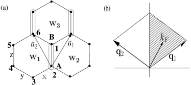
Figure 1: (a) Schematic of a fragment of the Kitaev lattice showing the $A$ and $B$ sites and the $x,$ $y$ and $z$ types of bonds. (b) Figure showing the reciprocal lattice vectors for the $A$ sublattice. The Dirac point for the massless Majorana fermions is denoted by $k_{F}$ and momentum summations are over the (shaded) half Brillouin zone.

For each $\alpha-$type bond, $u_{ij}^{\alpha}=ib_{i}^{\alpha}b_{j}^{\alpha}$ is also conserved and the flux operators can be written as a product of $u_{ij}$’s on the plaquette $\Pi_{\langle ij\rangle\in\text{Plaq.}}u_{ij}.$ The ground state manifold corresponds to a vortex-free state where all $W_{i}$ are equal. In the vortex-free state, we can fix all $u_{ij}=1$ (corresponds to $W_{p}=1$) and the Hamiltonian can be written as a tight-binding model of noninteracting Majorana fermions. The reduced Hamiltonian for this ground state manifold is given by $H_{0}=\frac{i}{4}\sum_{jk}A_{jk}c_{j}c_{k},$ where $A_{jk}=2J_{{\alpha}_{{}_{jk}}}$ if $j,\,k$ are neighboring sites on an $\alpha-$bond and zero otherwise. The excited states (with finite vorticity) are separated from the ground state manifolds by a gap of order $J_{\alpha}.$

The free Majorana fermion hopping Hamiltonian can be diagonalized in momentum space by defining the Bravais lattice with a two-point basis (Fig.1). In momentum space,

$$H_{0}= \frac{1}{4}\sum_{\mathbf{q}>0,\alpha}\epsilon_{\alpha}(\mathbf{q})a_{\mathbf{q},\alpha}^{\dagger}a_{\mathbf{q},\alpha},$$ (2)

with $\epsilon_{\alpha}(\mathbf{q})=\pm|f(\mathbf{q})|,\>\>f(\mathbf{q})=2i(J_{x}e^{ia_{0}\mathbf{q\cdot n_{1}}}+J_{y}e^{ia_{0}\mathbf{q\cdot n_{2}}}+J_{z})$, where $a_{0}$ is the nearest neighbor spin distance. The eigenstates are $a_{\mathbf{q},0}=\tilde{c}_{\mathbf{q},A}+\tilde{c}_{\mathbf{q},B}e^{-i\tilde{\alpha}(\mathbf{q})}$ and $a_{\mathbf{q},1}=\tilde{c}_{\mathbf{q},A}-\tilde{c}_{\mathbf{q},B}e^{-i\tilde{\alpha}(\mathbf{q})},$ with $\alpha(q)$ being the phase of $f(q).$

The Kitaev model has gapless excitations for a region of parameter space where $J_{\alpha}$’s satisfy the triangle inequalities $|J_{x}|+|J_{y}|\geq|J_{z}|$ etc. and a gapped spectrum outside this parameter regime. The gapless phase has a point Fermi surface where $\epsilon(\mathbf{k}_{F})=0$ and $\epsilon(\mathbf{q})$ has a linear dispersion around $\mathbf{k}_{F}$ (Fig.1). For simplicity, we will assume $J_{x}=J_{y}=J_{z}=J$ for further analysis. For this case, the Fermi points are at $(\pm 4\pi/3\sqrt{3}a_{0},0).$

The ground state of the Kitaev model is a quantum spin liquid with only nearest neighbor spin-spin correlations. baskaran07 On an $\alpha-$bond, only $\langle\sigma_{i}^{\alpha}\sigma_{j}^{\alpha}\rangle$ is non zero and other two spin correlations are zero. Four spin bond-bond correlations are long-ranged with power-law decay in the gapless phase of the Kitaev model.

III Topological Kondo effect

Consider a spin $S$ impurity locally exchange-coupled to a host (Kitaev) spin at an $A$ site ($\mathbf{r}=0$):

$$V_{K}= i\sum_{\alpha}K^{\alpha}S^{\alpha}b^{\alpha}c_{A}=i\sum_{\mathbf{q}\in HBZ,\alpha}\frac{K^{\alpha}}{\sqrt{2N}}S^{\alpha}b^{\alpha}(\tilde{c}_{\mathbf{q},A}+\tilde{c}_{\mathbf{q},A}^{\dagger})$$

$$\equiv \frac{1}{\sqrt{N}}\sum_{\mathbf{q}\in HBZ,\alpha,\beta}Q^{\alpha}S^{\alpha}b^{\alpha}(a_{\mathbf{q},\beta}+a_{\mathbf{q},\beta}^{\dagger}).$$ (3)

We perform a poor man’s scaling analysisanderson70 ; hewson92 for the Kondo coupling $K$ to study the screening of the impurity spin by the host excitations. To study the system properties at low temperatures, we can compute the effective Hamiltonian for a reduced bandwidth for the fermionic excitations ($-D+\delta D\text{ to }D-\delta D$) by integrating out the excitations in the band edges (($-D\text{ to }-D+\delta D)\text{ and }(D\text{ to }D-\delta D)$). This process is successively repeated to get a scaling law for the coupling constants in the Hamiltonian. We consider the Lippmann-Schwinger expansion for the $T-$matrix element, $\langle\Omega,b^{\beta}|K^{\beta}S^{\beta}b^{\beta}c_{a,A}|\Omega+(\mathbf{q},\alpha)\rangle.$ making a perturbation expansion $T=T^{(1)}+T^{(2)}+\cdots$ in increasing powers of $K$ and following its variation as a function of the decrease of the bandwidth $(-D,D),$ we find that the first correction to the bare $T-$matrix comes from two third order terms (see Fig. 2). The contribution from on-site scattering (Fig.2a) is

$$T^{(3),a} =\langle\Omega,b^{\beta}|V_{K}G_{0}^{+}(E)V_{{K}}G_{0}^{+}(E)V_{K}|\Omega+(\mathbf{q},\alpha)\rangle$$

$$\!\!\!\!\!\!\!\!\!\!\!\!\!\!\!=\frac{Q^{\beta}S^{\beta}}{N}\!\!\!\!\!\!\!\!\!\sum_{(D-\delta D)\leq|\epsilon_{q^{\prime}}|,|\epsilon_{q^{\prime\prime}}|\leq D,\tilde{\alpha},\tilde{\beta},\tilde{\alpha}^{\prime}}\!\!\!\!\!\!\!\!\!\!\!\!\!\!\!\!\!\!\!\!\!(Q^{\tilde{\beta}})^{2}(S^{\tilde{\beta}})^{2}\langle b^{\beta}|\>b_{\beta}^{\dagger}(a_{\mathbf{q}^{\prime\prime},\tilde{\alpha}^{\prime}}+a_{\mathbf{q}^{\prime\prime},\tilde{\alpha}^{\prime}}^{\dagger})$$

$$\hskip 14.22636pt\times G_{0}^{+}(\epsilon)\>b_{\tilde{\beta}}(a_{\mathbf{q}^{\prime},\tilde{\alpha}}+a_{\mathbf{q}^{\prime},\tilde{\alpha}}^{\dagger})\>G_{0}^{+}(\epsilon)\>b_{\tilde{\beta}}^{\dagger}c_{\mathbf{q},\alpha}|(\mathbf{q},\alpha)\rangle$$

$$\!\!\!\!\!\!\!\!\!\!\!\!\!\!\!\!\!\!\!\!=-\frac{Q^{\beta}S^{\beta}}{N}\!\sum_{\mathbf{q}^{\prime},\tilde{\beta}}(Q^{\tilde{\beta}})^{2}(S^{\tilde{\beta}})^{2}\left\langle a_{\mathbf{q}^{\prime},1}^{\dagger}a_{\mathbf{q}^{\prime},1}\frac{1}{E-(H_{0}-\epsilon_{q^{\prime},1})}\right.$$

$$\hskip 51.21504pt\left.+a_{\mathbf{q}^{\prime},0}a_{\mathbf{q}^{\prime},0}^{\dagger}\frac{1}{E-(H_{0}+\epsilon_{q^{\prime},0})}\right\rangle\!\frac{1}{E-\epsilon_{b}}\>$$

$$\!\!\!\!\!\!\!\!\!\!\!\!\!\!\!\simeq-2Q^{\beta}S^{\beta}\frac{\rho(D)a^{2}|\delta D|}{E-D}\cdot\frac{1}{E-J}\sum_{\tilde{\beta}}(Q^{\tilde{\beta}})^{2}(S^{\tilde{\beta}})^{2}.$$ (4)

Here $\rho(D)$ is the density of states at the band edge, $a$ is the lattice constant and $G_{0}(E)=(E-H_{0}+i\delta)^{-1}.$

Similarly, the contribution from Fig. 2(b) is

$$T^{(3),b} =\frac{Q^{\beta}S^{\beta}}{N}\!\!\!\!\!\!\!\!\!\!\!\!\!\!\!\!\!\!\!\!\!\!\!\!\!\!\!\sum_{(D-\delta D)\leq|\epsilon_{q^{\prime}}|,|\epsilon_{q^{\prime\prime}}|\leq D,\tilde{\alpha},\tilde{\beta},\tilde{\alpha}^{\prime}}\!\!\!\!\!\!\!\!\!\!\!\!\!\!\!\!\!\!\!\!\!\!\!\!\!\!\!(Q^{\tilde{\beta}})^{2}(S^{\tilde{\beta}})^{2}\langle b^{\beta}|\>b_{\tilde{\beta}}^{\dagger}(a_{\mathbf{q},{\alpha}}+a_{\mathbf{q},{\alpha}}^{\dagger})$$

$$\times G_{0}^{+}(\epsilon)\>b_{\tilde{\beta}}(a_{\mathbf{q}^{\prime},\tilde{\alpha}}+a_{\mathbf{q}^{\prime},\tilde{\alpha}}^{\dagger})\>G_{0}^{+}(\epsilon)\>b_{{\beta}}^{\dagger}(a_{\mathbf{q}^{\prime},\tilde{\alpha}}+a_{\mathbf{q}^{\prime},\tilde{\alpha}}^{\dagger})|(\mathbf{q},\alpha)\rangle$$

$$=-\frac{Q^{\beta}S^{\beta}}{N}\!\!\!\!\!\!\!\!\!\!\!\!\!\!\!\!\!\!\!\!\!\!\!\!\!\sum_{(D-\delta D)\leq|\epsilon_{q^{\prime}}|,|\epsilon_{q^{\prime\prime}}|\leq D,\tilde{\alpha},\tilde{\beta},\tilde{\alpha}^{\prime}}\!\!\!\!\!\!\!\!\!\!\!\!\!\!\!\!\!\!\!\!\!\!\!\!(Q^{\tilde{\beta}})^{2}(S^{\tilde{\beta}})^{2}\>\langle\Omega,b^{\beta}|\>b_{\tilde{\beta}}^{\dagger}c_{\mathbf{q},\alpha}b^{\dagger}_{\beta}c^{\dagger}_{\mathbf{q},\alpha}\>$$

$$\times\frac{1}{E-(H_{0}+\epsilon_{b}+\epsilon_{q,0})}\>b_{\tilde{\beta}}(a_{\mathbf{q}^{\prime},\tilde{\alpha}}+a^{\dagger}_{\mathbf{q}^{\prime},\tilde{\alpha}})$$

$$\times\frac{1}{E-(H_{0}+\epsilon_{b}+\epsilon_{q,0})}\>(a_{\mathbf{q}^{\prime},\tilde{\alpha}}+a^{\dagger}_{\mathbf{q}^{\prime},\tilde{\alpha}})|\Omega\rangle$$

$$= -\frac{Q^{\beta}S^{\beta}}{N}\sum_{\mathbf{q}^{\prime},\tilde{\beta}}(Q^{\tilde{\beta}})^{2}(S^{\tilde{\beta}})^{2}\>\frac{1}{E-2\epsilon_{b}}\>$$

$$\hskip 11.38092pt\times\langle a^{\dagger}_{\mathbf{q}^{\prime},1}a_{\mathbf{q}^{\prime},1}\frac{1}{E-(-\epsilon_{q^{\prime},1}+\epsilon_{b}+\epsilon_{q,0})}$$

$$\hskip 11.38092pt+a_{\mathbf{q}^{\prime},0}a^{\dagger}_{\mathbf{q}^{\prime},0}\frac{1}{E-(\epsilon_{q^{\prime},0}+\epsilon_{b}+\epsilon_{q,0})}\rangle$$

$$\simeq-2Q^{\beta}S^{\beta}\>\frac{\rho(D)a^{2}|\delta D|}{E-D-J}\cdot\frac{1}{E-2J}\sum_{\tilde{\beta}}(Q^{\tilde{\beta}})^{2}(S^{\tilde{\beta}})^{2}.$$ (5)

Figure 2: Diagrams contributing to the scaling of Kondo coupling $K^{\alpha}$.

Adding the two contributions (taking $E\simeq 0$),

$$T^{(3)} \simeq 2Q^{\beta}S^{\beta}\rho(D)\frac{a^{2}\delta D}{\epsilon_{b}}\sum_{\tilde{\beta}}(Q^{\tilde{\beta}})^{2}(S^{\tilde{\beta}})^{2}\left\{\frac{1}{D}+\frac{1}{2(D+J)}\right\}.$$ (6)

Here we have taken $E,\epsilon_{q,\alpha}\ll D,\,J$ and neglected them.

If either the impurity is a $S=\frac{1}{2}$ spin, or the Kondo interaction is rotationally symmetric, the above contribution renormalizes the Kondo coupling constant. However for $S\neq\frac{1}{2}$ with anisotropic coupling, new terms are generated and one needs to go to higher order diagrams to obtain the scaling of these new coupling terms. For $S=1/2$ or for symmetric impurity coupling we thus have

$$\delta K \sim-2K^{3}S(S+1)\rho(D)a^{2}\frac{\delta D}{J}\left\{\frac{1}{D}+\frac{1}{2(D+J)}\right\}.$$ (7)

Just as for the Kondo effect in graphenewithoff90 , owing to the change in the density of states with bandwidth (here $\rho(\epsilon)=(1/2\pi v_{F}^{2})|\epsilon|\equiv C|\epsilon|$), we also need to consider the change in $K$ due to the rescaling done in order to keep the total number of states fixed. This gives a contribution $K\rightarrow K(D^{\prime}/D),\quad(D^{\prime}=D-|\delta D|).$ In addition, as we shall scale the bandwidth $D$ to smaller values, the second term in Eq. 7 may be dropped. Thus

$$\delta K \simeq-2K^{3}S(S+1)\rho(D)a^{2}\frac{\delta D}{DJ}+K\frac{\delta D}{D}$$

$$=-K\frac{\delta D}{D}\left(2K^{2}a^{2}CDS(S+1)/J-1\right).$$ (8)

Thus, as we decrease the bandwidth by integrating out the high energy excitations, the effective coupling $K$ has an unstable fixed point at $K_{c}=\sqrt{J/[2a^{2}\rho(D)S(S+1)]};$ or in other words, $K_{c}\sim\sqrt{J/S^{2}a^{2}CD}\sim J/S.$ Here we used $D\lesssim J$ and $C\sim 1/(Ja)^{2}.$ Clearly for $K>K_{c},$ the coupling flows to infinity independent of the nature of coupling (ferromagnetic or antiferromagnetic), while for $K<K_{c},$ the coupling flows to zero. For anisotropic Kondo coupling we can show

$$\delta K_{z,\pm} \sim-K_{z,\pm}\frac{\delta D}{D}\left[2a^{2}\rho(D)S(S+1)\frac{K_{z}^{2}+K_{+}K_{-}}{J}-1\right].$$ (9)

The two-parameter Kondo flow is therefore given by

$$\frac{\delta K_{z}}{\delta K_{\pm}}=\frac{K_{z}}{K_{\pm}}\Rightarrow\frac{K_{z}}{K_{\pm}}=\text{const}.$$ (10)

A comparison of the Kondo effect in graphene withoff90 , a bosonic spin bath florens06 and the Kitaev model are shown in Table 1.

	Graphene	$Z_{2}$ bosonic spin bath with pseudogap density of states $\rho(\epsilon)=C|\epsilon|.$	Kitaev, honeycomb lattice
Kondo scaling	Unstable intermediate coupling fixed pt. only for AFM coupling. Only AFM flows to strong coupling above unstable fixed pt.	Flow direction is independent of the sign of magnetic impurity coupling. Unstable intermediate coupling fixed pt. for both FM and AFM.	Scaling same as $Z_{2}$ bosonic spin bath case. However a topological transition is associated with the unstable fixed point.

Table 1: Comparison of Kondo effect in graphene, a $Z_{2}$ bosonic spin bath with a pseudogap density of states and the Kitaev model on the honeycomb lattice.

III.1 Stability of strong coupling point

The poor man’s scaling analysis is only valid for small Kondo couplings as the perturbation theory breaks down much before the critical value of the coupling. While we have shown that the coupling flows to larger values above the critical value $K_{c},$ it remains to be seen whether there is any other fixed point beyond $K_{c}$ but less than the $\infty.$ Below we study the model in the strong coupling limit and see if it is a stable fixed point. In the strong coupling limit, $K$ is the largest energy scale and the impurity spins forms a singlet/triplet with the Kitaev spin at origin.

We consider the Hamiltonian such that the Kondo term and the Kitaev model with one spin missing ($H_{K-}$) constitute the unperturbed Hamiltonian and Kitaev coupling to the site at origin is the perturbation:

$$H_{0} =K\mathbf{S}\cdot\mathbf{\sigma}_{0}+H_{K-},$$ (11)

$$V =J(\sigma_{0}^{x}\sigma_{1}^{x}+\sigma_{0}^{y}\sigma_{2}^{y}+\sigma_{0}^{z}\sigma_{3}^{z}).$$ (12)

For antiferromagnetic Kondo coupling ($K>0$), the ground state consists of a Kondo singlet of $S\text{ and }\sigma_{0}$ and the Kitaev model with one spin missing. The perturbation term causes transitions from singlet to triplet states of the Kondo singlet. We use effective Hamiltonian schemeprimas63 to include the effects of the perturbation terms within the projected ground state subspace.

$$H_{\text{eff}}=\text{e}^{iQ}H\text{e}^{-iQ},$$ (13)

where $Q$ is chosen such that the terms which take us out of the reduced Hilbert space are canceled order by order. This gives the reduced Hamiltonian as

$$H_{\text{eff}}=H_{0}+H_{1}+H_{2}+O(V^{3}),$$ (14)

$$\langle\alpha|H_{1}|\beta\rangle=\langle\alpha|V|\beta\rangle,$$ (15)

$$\langle\alpha|H_{2}|\beta\rangle=\frac{1}{2}\!\!\!\sum_{\gamma\neq\alpha,\beta}\!\!\!\langle\alpha|V|\gamma\rangle\langle\gamma|V|\beta\rangle\!\left(\frac{1}{E_{\alpha}-E_{\gamma}}+\frac{1}{E_{\beta}-E_{\gamma}}\!\right)\!,$$ (16)

where $\alpha,\beta$ belong to the ground state manifold and $\gamma$ belongs to excited state manifold. The eigenstates of the Kondo term are singlet $|s\rangle$ and triplet states $|t,(0,\pm 1)\rangle$:

$$|s\rangle=\frac{1}{\sqrt{2}}\left(|\uparrow,\Downarrow\rangle-|\downarrow,\Uparrow\rangle\right),$$ (17)

$$|t,1\rangle=|\uparrow,\Uparrow\rangle,$$ (18)

$$|t,0\rangle=\frac{1}{\sqrt{2}}\left(|\uparrow,\Downarrow\rangle+|\downarrow,\Uparrow\rangle\right),$$ (19)

$$|t,-1\rangle=|\downarrow,\Downarrow\rangle.$$ (20)

Here $\uparrow$ refers to the Kitaev spin and $\Uparrow$ refers to the impurity spin state.

Antiferromagnetic Kondo coupling

For the antiferromagnetic Kondo coupling case, ground state is the singlet state. As $\langle s|V|s\rangle=0$, $H_{1}=0$ and

$$\langle s,K_{-}|H_{2}|s,K_{-}^{\prime}\rangle=\frac{1}{2}\sum_{t,K_{-}^{\prime\prime}}\langle s,K_{-}|V|t,K_{-}^{\prime\prime}\rangle$$

$$\hskip 28.45274pt\times\langle t,K_{-}^{\prime\prime}|V|s,K_{-}^{\prime}\rangle\left(\frac{1}{E_{0}-E_{t}}+\frac{1}{E_{0}^{\prime}-E_{t}}\right).$$ (21)

Here, $K_{-}$ denotes the eigenstates of the Kitaev model with the spin at origin missing. Since change in energy of the Kitaev state is $\sim J\ll K$, we ignore their contribution in the energy denominators of the perturbation term. The matrix elements of $H_{2}$ are then

$$\langle s,K_{-}|H_{2}|s,K_{-}^{\prime}\rangle$$ (22)

$$\simeq\frac{J^{2}}{E_{0}-E_{t}}\!\!\!\sum_{t,K_{-}^{\prime\prime},\alpha,\beta}\!\!\!\!\!\!\langle s|\sigma_{0}^{\alpha}|t\rangle\langle t|\sigma_{0}^{\beta}|s\rangle\langle K_{-}|\sigma_{\alpha}^{\alpha}|K_{-}^{\prime\prime}\rangle\langle K_{-}^{\prime\prime}|\sigma_{\beta}^{\beta}|K_{-}^{\prime}\rangle$$ (23)

$$\simeq-\frac{J^{2}}{K}\sum_{\alpha,\beta}\langle s|\sigma_{0}^{\alpha}(\mathbf{1}-|s\rangle\langle s|)\sigma_{0}^{\beta}|s\rangle\langle K_{-}|\sigma_{\alpha}^{\alpha}\sigma_{\beta}^{\beta}|K_{-}^{\prime}\rangle$$ (24)

$$=-\frac{3J^{2}}{K}\sum_{\alpha,\beta}\langle K_{-}|\sigma_{\alpha}^{\alpha}\sigma_{\beta}^{\beta}|K_{-}^{\prime}\rangle.$$ (25)

Here, in $\sigma_{\alpha}^{\alpha},$ the subscript $\alpha$ refers to a neighoring site of the origin in the direction of the $\alpha-$bond. Thus, in the antiferromagnetic coupling case, the Kondo singlet decouples from the rest of the Kitaev model and a small interaction ($J^{2}/K\ll J$) is generated between the Kitaev spin at the origin and the sins at the three neighboring sites in the second order perturbation. The strong coupling fixed point is thus a stable fixed point and is equivalent to the Kitaev model with one site missing.

Ferromagnetic Kondo coupling

In the ferromagnetic Kondo coupling case, the triplet states form the ground state manifold. We perform degenerate perturbation theory to get the effective Hamiltonian:

$$\langle t^{\prime},K_{-}^{\prime}|H_{1}|t,K_{-}\rangle =J\langle t^{\prime},K_{-}^{\prime}|V|t,K_{-}\rangle$$ (26)

$$=\sum_{\alpha}\langle t^{\prime}|\sigma_{0}^{\alpha}|t\rangle\langle K_{-}^{\prime}|\sigma_{\alpha}^{\alpha}|K_{-}\rangle.$$ (27)

If we calculate the matrix elements of $\langle t^{\prime}|\sigma_{0}^{\alpha}|t\rangle,$ these matrices are just the spin$-1$ matrices:

$$\sigma_{0}^{x} =\left(\begin{array}[]{ccc}0&\frac{1}{\sqrt{2}}&0\\ \frac{1}{\sqrt{2}}&0&\frac{1}{\sqrt{2}}\\ 0&\frac{1}{\sqrt{2}}&0\end{array}\right),$$

$$\sigma_{0}^{y} =\left(\begin{array}[]{ccc}0&-\frac{i}{\sqrt{2}}&0\\ \frac{i}{\sqrt{2}}&0&-\frac{i}{\sqrt{2}}\\ 0&\frac{i}{\sqrt{2}}&0\end{array}\right),$$

$$\sigma_{0}^{z} =\left(\begin{array}[]{ccc}1&0&0\\ 0&0&0\\ 0&0&-1\end{array}\right)$$

and the Hamiltonian in the reduced subspace becomes

$$H_{1}=JS_{0}^{\alpha}\sigma_{\alpha}^{\alpha}.$$ (28)

where $\mathbf{S}_{0}$ represents the spin-1 at the origin.

Thus for ferromagnetic impurity coupling, the new terms which couple the triplet and the rest of the Kitaev model are similar to the original Kitaev coupling and of the same strength. We get a Kitaev-like model with a spin$-1$ at the origin and spin$-1/2$ elsewhere. Here the Kondo triplet does not decouple from rest of the Kitaev model in the strong coupling limit and does not lend itself to a simple treatment, unlike the corresponding antiferromagnetic case.

III.2 Topological transition

A remarkable property of the Kondo effect in Kitaev model is that the unstable fixed point is associated with a topological transition from the zero flux state to a finite flux state. The strong antiferromagnetic coupling limit amounts to studying the Kitaev model with a missing site or cutting the three bonds linking this site to the neighbors. It was shown in Kitaev’s original paperkitaev06 that such states with an odd number of cuts are associated with a finite flux, and also that these vortices are associated with unpaired Majorana fermions and have non-abelian statistics under exchange. It has also been shown numerically for the gapless phasewillans10 that the ground state of the Kitaev model with one spin missing has a finite flux pinned to the defect site. We argue the existence of a localized zero energy Majorana mode from the degeneracy of the ground state in presence of impurity spin and elucidate on the nature of this zero mode.

For the Hamiltonian $H=H_{0}+V_{K},$ the three plaquettes $W_{1},$ $W_{2}$ and $W_{3}$ (Fig. 3) that touch the impurity site are no longer associated with conserved flux operators, while the flux operators that do not include the origin remain conserved. The three plaquette operator $W_{0}=W_{1}W_{2}W_{3}$ is still conserved and $W_{0}=1$ in the ground state of the unperturbed Kitaev model.

We now define composite operators $\tau^{x}=W_{2}W_{3}S^{x},$ $\tau^{y}=W_{3}W_{1}S^{y}$ and $\tau^{z}=W_{1}W_{2}S^{z}$ ( $S^{\alpha}$ are the Pauli spin matrices corresponding to the impurity). Remarkably, these composite operators represent conserved quantities for arbitrary values of the impurity coupling. The $\tau^{\alpha}$’s do not commute with each other and instead obey an $SU(2)$ algebra, $[\tau^{\alpha},\tau^{\beta}]=2i\epsilon_{\alpha\beta\gamma}\tau^{\gamma}.$ This $SU(2)$ symmetry, which is exact for all couplings is realized in the spin-1/2 representation $\left(\left(\tau^{\alpha}\right)^{2}=1\right)$. Clearly, all eigenstates, including the ground state are doubly degenerate (corresponding to $\tau^{z}=\pm 1$), and this applies also to the strong coupling limit.

Figure 3: Schematic of the three unpaired b–Majorana fermions formed as a result of cutting the links to the Kitaev spin at the origin. Any two of the three can be given an expectation value (dotted bond).

In the strong antiferromagnetic coupling limit $J_{K}\rightarrow\infty,$ the low energy states will be the ones in which the spin at the origin forms a singlet $|0\rangle$ with the impurity spin, $|\psi\rangle=|\psi K^{-}\rangle\otimes|0\rangle.$ Here $|\psi K^{-}\rangle$ represents the low energy states of the Kitaev model with the spin at the origin removed. To see the action of the $SU(2)$ symmetry generators on these states, we note that they can be written as $\tau^{\alpha}=\tilde{W}^{\alpha}\otimes\sigma_{0}^{\alpha}\otimes S^{\alpha}$ and $\tilde{W}^{\alpha}$ do not involve the components of the spin at the origin, $\sigma_{0}^{\alpha}.$ We then have $\tau^{\alpha}|\psi\rangle=-(\tilde{W}^{\alpha}|\psi K^{-}\rangle)\otimes|0\rangle$. So, in the strong coupling limit, the symmetry generators act non-trivially only in the Kitaev model sector, implying that the low energy states of the Kitaev model with one spin removed are all doubly degenerate, with the double degeneracy emerging from the Kitaev sector. This is also true for the zero-energy mode in the single particle spectrum: the two degenerate states correspond to the zero mode being occupied or unoccupied.

Let us examine the structure of the zero mode. Removing a Kitaev spin creates three unpaired $b-$Majorana fermions at the neighboring sites, say, $b_{3}^{z},$ $b_{1}^{x}$ and $b_{2}^{y}$ (Fig. 3). Now $ib_{1}^{x}b_{2}^{y}$ is conserved and commutes with all the conserved flux operators $W_{i}$ but not with the two other combinations $ib_{2}^{y}b_{3}^{z}$ and $ib_{3}^{z}b_{1}^{x}.$ So, we can choose a gauge where the expectation value of $ib_{1}^{x}b_{2}^{y}$ is equal to +1 such that these two $b-$modes drop out of the problem and we equivalently have one unpaired $b-$Majorana fermion. The unpaired $b_{3}^{z}$ Majorana has dimension $\sqrt{2}$ and therefore, there must be an unpaired Majorana mode in the $c-$sector (again of dimension $\sqrt{2}$) so that together these two give the full (doubly degenerate) zero energy mode. Also, while the $b_{3}^{z}$ mode is sharply localized, the wave function of the $c$ mode can be spread out in the lattice.

For the ferromagnetic case, while the strong coupling limit also leads to a model with doubly-degenerate levels, we are unable to explicitly identify a zero energy unpaired Majorana fermion and not address the question as to whether a nontrivial $Z_{2}$ flux can be associated with closed paths enclosing the $S=1$ defect. For this purpoose, we perform a numerical exact diagonalization analysis below.

IV Numerical studies

We have used a modified Lanczos algorithm to calculate the ground state properties of a finite Kitaev fragment exchange-coupled to an external $S=1/2$ impurity spin as discussed in the previous sections.

For the antiferromagnetic case, where we already know that the strong-coupling limit $K/J\rightarrow\infty$ is associated with a nontrivial flux $W_{0}=-1$ at the defect site, an exact-diagonalization calculation with a fragment as small as three hexagons (open boundary conditions, impurity spin coupled to central site) is sufficient to confirm $W_{0}=-1.$ Figure 4 shows the expectation value of the flux operator $W$ and total spin $S_{Tot}=S+s_{i}$ as a function of the impurity coupling $K.$ It is seen that the $W_{0}=1$ for $K=0$ (i.e in the pure Kitaev case) as it should be, since the ground state of Kitaev model is flux free, whereas it changes to -1 as $K$ is increased, implying a finite $Z_{2}$ flux at the origin. Within numerical accuracy, it also appears that the topological transition from $W_{0}=1$ to $W_{0}=-1$ practically occurs at the same value of $K$ at which a bound singlet state is formed between the impurity spin and the Kitaev host. For negative values of $K$ for this three-hexagon fragment, $W_{0}$ appears to stay close to one implying a flux-free state even as the total spin at the defect site begins approaching $S=1.$ We suspect this anomalous result is not generally true for larger fragments and may have originated from the presence of a large number of boundary spins that interact with the central spin. We thus performed exact-diagonalization calculations with a larger fragment with six hexagons (open boundary conditions, impurity spin coupled to central site). As we increase the ferromagnetic impurity coupling, we clearly observe the $W_{0}=1$ to $W_{0}=-1$ topological transition. Once again, the topological phase transition and the magnetic transition (at which the total spin at the defect site becomes $S=1,$ are practically coincident.

Figure 4: (Color online) (Top) Evolution of expectation value of the flux operator ($W_{0}$) and the total spin at the impurity site with $K$ evaluated on a three hexagon fragment. The impurity spin is coupled to the central spin and the flux is calculated over the boundary. The inset shows the slight decrease of $W_{0}$ from 1 for ferromagnetic coupling whereas for antiferromagnetic coupling $W_{0}$ changes to -1. (Bottom) $W_{0}$ and total spin at the impurity site evaluated for a six hexagon fragment showing the transition to $W_{0}$ = -1 state for ferromagnetic coupling.

V Two-channel Kondo behavior

In Ref. willans10, , the temperature and magnetic field dependences of the magnetic susceptibility of the Kitaev model with a missing site were obtained as $\chi_{\text{imp}}(T)\sim\ln(1/T)$ and $\chi_{\text{imp}}(h)\sim\ln(1/h),$ respectively, which bears striking resemblance to the low-temperature impurity susceptibility in the two-channel Kondo model emery ; sengupta . This is not a mere coincidence. In the two-channel Kondo problem, it is long known coleman1995 that the low energy physics is described by a model of a localized, zero energy Majorana fermion interacting with a band of dispersing Majorana fermions with a finite density of states at the Fermi energy. Likewise, in the Kitaev model with a missing site, we can clearly identify a localized zero energy Majorana $b-$fermion coexisting with dispersing Majorana $c-$fermions with a nonvanishing density of states willans10 at zero energy. A nonvanishing density of states for the dispersing Majoranas is a very unusual result for a honeycomb lattice, and is associated with the fact that the missing site is associated with a finite $Z_{2}$ flux. If one instead estimates the density of states for the dispersing fermions in the absence of a $\pi-$flux, the density of states would vanish willans10 at the Fermi energy; indeed, this would be the case in graphene. To compute the magnetic susceptibility, we choose a gauge where $b_{3}^{z}$ is the zero energy localized Majorana fermion. Using $S_{3}^{z}=ic_{3}b_{3}^{z}$ the magnetic susceptibility of the defect can be expressed as

$$\chi_{\text{imp}}=T\sum_{n,k}\frac{1}{i\nu_{n}-\epsilon_{k}}\frac{1}{i\nu_{n}}\sim\ln(1/T),$$ (29)

where $(i\nu_{n}-\epsilon_{k})^{-1}$ and $1/i\nu_{n}$ are respectively the Green functions of the dispersing and the (zero-energy) localized Majorana fermions and we used the fact that the density of states of the dispersing Majorana fermions does not vanish at zero energy. For finite fields $h$ in the low temperature limit, the logarithmic divergence of Eq.29 gets cut off by the field, and one obtains $\chi_{\text{imp}}(h)\sim\ln(1/h).$ For the ground state entropy, one notes that the dispersing Majorana fermions have zero entropy at $T=0$ while the localized zero energy Majorana fermion has a finite entropy $S=(1/2)\ln(2).$ This again agrees with the two-channel Kondo result.emery

VI Discussion

In summary, we showed that the problem of spinless and spinful defects in the honeycomb $S=1/2$ Kitaev model can be approached from a more general “Kondo perspective” of local exchange coupling of external paramagnetic impurities with a host spin. On one hand, such an approach gives us a new class of Kondo effects where the magnetic binding-unbinding transition is accompanied by a change of topology of the ground state. On the other hand, some intriguing recent observations, such as logarithmic singularities in the magnetic response of Kitaev models with vacancies, are now recognizable as familiar Kondo stories - in this case, we note a remarkable similarity with the two-channel Kondo problem. It would be interesting to study a lattice of vacancies in the Kitaev model from the perspective of a two-channel Kondo lattice. One would like to better understand the Kitaev model with a $S=1$ defect. This nonintegrable nature of this problem prevents us from repeating the kind of analysis one could make for the vacancy case where similarity with the two-channel Kondo problem was observed. Our numerical approach, based on exact diagonalization calculations of relatively small fragments, cannot answer questions such as the density of states of low energy excitations. Another direction for future study would be to consider a more general Kitaev-Heisenberg model and track the Kondo effect as a function of the relative strengths of Kitaev and Kondo interactions. This should give insights into magnetic impurity response in Kitaev candidate materials where Kitaev and Heisenberg interactions are believed to compete with each other.

- (1) A. I. Larkin and V. I. Mel’nikov, JETP 656 (1972).
- (2) H. Maebashi, K. Miyake, and C. M. Varma, Phys. Rev. Lett. 88, 226403 (2002).
- (3) Y. L. Loh, V. Tripathi, and M. Turlakov, Phys. Rev. B 71, 024429 (2005).
- (4) G. Khaliullin, R. Kilian, S. Krivenko, P. Fulde, Phys. Rev B 56, 11882 (1997).
- (5) A. Kolezhuk, S. Sachdev, R. R. Biswas, and P. Chen, Phys. Rev. B 74, 165114 (2006).
- (6) S. Florens, L. Fritz, M. Vojta, Phys. Rev. Lett. 96, 036601 (2006).
- (7) A. Yu. Kitaev, Ann. Phys. (Berlin) 321, 2 (2006).
- (8) G. Baskaran, S. Mandal, and R. Shankar, Phys. Rev. Lett. 98, 247201 (2007).
- (9) G. Jackeli, and G. Khaliullin, Phys. Rev. Lett. 102, 017205 (2009).
- (10) L.-M. Duan, E. Demler, and M. D. Lukin, Phys. Rev. Lett. 91, 090402 (2003).
- (11) Kusum Dhochak, R. Shankar, and V. Tripathi, Phys. Rev. Lett. 105, 117201 (2010).
- (12) D. Withoff and E. Fradkin, Phys. Rev. Lett. 64, 1835 (1990).
- (13) A.J. Willans, J. T. Chalker, R. Moessner, Phys. Rev. Lett. 104, 237203 (2010).
- (14) Fabien Trousselet, Giniyat Khaliullin, and Peter Horsch, Phys. Rev. B 84, 054409 (2011).
- (15) A. J. Willans, J. T. Chalker, and R. Moessner, Phys. Rev. B 84, 115146 (2011).
- (16) P. Coleman, L. B. Ioffe, and A. M. Tsvelik, Phys. Rev. B 52, 6611 (1995).
- (17) P. W. Anderson, J. Phys. C: Solid State Phys. 3 2436 (1970).
- (18) A. Hewson, The Kondo Problem to Heavy Fermions, Cambridge University Press, Cambridge, 1992.
- (19) S. Saremi, Phys. Rev. B 76, 184430 (2007).
- (20) H. Primas, Rev. Mod. Phys. 35, 710 (1963); Arnab Sen, Frustrated Antiferromagnets with Easy Axis Anisotropy, Ph.D. Thesis, Tata Institute of Fundamental Research, Mumbai, 2009.
- (21) G. Santhosh, V. Sreenath, A. Lakshminarayan and R. Narayanan, Phys. Rev. B 85, 054204 (2012).
- (22) X.-Y. Feng, G. M. Zhang, and T. Xiang, Topological Characterization of Quantum Phase Transitions in a Spin-1/2 Model, Phys. Rev. Lett. 98, 087204 (2007).
- (23) S. Dusuel, K. P. Schmidt, and J. Vidal, Creation and Manipulation of Anyons in the Kitaev Model, Phys. Rev. Lett. 100, 177204 (2008).
- (24) K. Sengupta, D. Sen, and S. Mondal, Exact Results for Quench Dynamics and Defect Production in a Two-Dimensional Model, Phys. Rev. Lett. 100, 077204 (2008).
- (25) D. H. Lee, G. M. Zhang, and T. Xiang, Edge Solitons of Topological Insulators and Fractionalized Quasiparticles in Two Dimensions, Phys. Rev. Lett. 99, 196805 (2007).
- (26) J. Q. You, X.-F. Shi, X. Hu, and F. Nori, Quantum emulation of a spin system with topologically protected ground states using superconducting quantum circuits, Phys. Rev. B 81, 014505 (2010).
- (27) D. A. Ivanov, Non-Abelian Statistics of Half-Quantum Vortices in p-Wave Superconductors, Phys. Rev. Lett. 86, 268 (2001).
- (28) Y. Yu , An exactly soluble model with tunable p-wave paired fermion ground states, Europhys. Lett., 84, 57002 (2008).
- (29) H. Alloul, Susceptibility and Electron-Spin Relaxation of Fe in Cu below : A NMR Study of 63Cu Satellites, Phys. Rev. Lett. 35, 460 (1975).
- (30) Feng Ye,Songxue Chi,Huibo Cao,Bryan C. Chakoumakos,Jaime A. Fernandez-Baca,Radu Custelcean,T. F. Qi,O. B. Korneta,and G. Cao Phys. Rev B 85, 180403(R) (2012)
- (31) Jir Chaloupka,George Jackeli,and Giniyat Khaliullin Phys. Rev. Lett 110,097204 (2013).
- (32) V. J. Emery and S. Kivelson, Phys. Rev. B 46, 10812 (1992).
- (33) A. M. Sengupta and A. Georges, Phys. Rev. B 49, 10020(R) (1994).
- (34) A. Banerjee, C.A. Bridges, J-Q Yan, A.A. Aczel, L.Li, M.B.Stone, G.E. Granroth, M.D. Lumsden, Y.Yui, J.Knolle, D. L. Kovrizhin, S.Bhattacharjee, R. Moessner, D.A.Tennant,D.G.Mandrus,and S.E.Nagler , arxiv 1504.08037,(2015).