Subsampling for General Statistics under Long Range Dependence with application to change point analysis

Abstract.

In the statistical inference for long range dependent time series the shape of the limit distribution typically depends on unknown parameters. Therefore, we propose to use subsampling. We show the validity of subsampling for general statistics and long range dependent subordinated Gaussian processes which satisfy mild regularity conditions. We apply our method to a self-normalized change-point test statistic so that we can test for structural breaks in long range dependent time series without having to estimate any nuisance parameter. The finite sample properties are investigated in a simulation study. We analyze three data sets and compare our results to the conclusions of other authors.

1. Introduction

1.1. Long Range Dependence

While most statistical research is done for independent data or short memory time series, in many applications there are also time series with long memory in the sense of slowly decaying correlations: in hydrology (starting with the work of Hurst [31]), in finance (e.g. Lo [39]), in the analysis of network traffic (e.g. Leland, Taqqu, Willinger and Wilson [37]) and in many other fields of research.

As model of dependent time series we will consider subordinated Gaussian processes: Let $(\xi_{n})_{n\in{\mathds{N}}}$ be a stationary sequence of centered Gaussian variables with ${\rm Var}(\xi_{n})=1$ and covariance function $\gamma$ satisfying

(1) $$\gamma(k):={\rm Cov}(\xi_{1},\xi_{k+1})=k^{-D}L_{\gamma}(k)$$

for $D>0$ and a slowly varying function $L_{\gamma}$. If $D<1$, the spectral density $f$ of $(\xi_{n})_{n\in{\mathds{N}}}$ is not continuous, but has a pole at $0$. The spectral density has the form

$$f(x)=|x|^{D-1}L_{f}(x)$$

for a function $L_{f}$ which is slowly varying at the origin (see Proposition 1.1.14 in Pipiras and Taqqu [44]).

Furthermore, let $G:{\mathds{R}}\rightarrow{\mathds{R}}$ be a measurable function such that $\operatorname{E}[G^{2}(\xi_{1})]<\infty$. The stochastic process $(X_{n})_{n\in{\mathds{N}}}$ given by

$$X_{n}:=G(\xi_{n})$$

is called long range dependent if $\sum_{n=0}^{\infty}|{\rm Cov}(X_{1},X_{n+1})|=\infty$, and short range dependent if $\sum_{n=0}^{\infty}|{\rm Cov}(X_{1},X_{n+1})|<\infty$.

In limit theorems for the partial sum $S_{n}=\sum_{i=1}^{n}X_{i}$, the normalization and the shape of the limit distribution not only depend on the decay of the covariances $\gamma(k)$ as $k\rightarrow\infty$, but also on the function $G$. More precisely, Taqqu [53] and Dobrushin and Major [25] independently proved that

$$\frac{1}{L_{\gamma}(n)^{r/2}n^{H}}\sum_{i=1}^{n}\left(X_{i}-\operatorname{E}[X_{i}]\right)\Rightarrow C(r,H)g_{r}Z_{r,H}(1)$$

if the Hurst parameter $H:=\max\{1-\frac{rD}{2},\frac{1}{2}\}$ is greater than $\frac{1}{2}$. Here, $r$ denotes the Hermite rank of the function $G$, $C(r,H)$ is a constant, $g_{r}$ is the first non-zero coefficient in the expansion of $G$ as a sum of Hermite polynomials and $Z_{r,H}$ is a Hermite process. For more details on Hermite polynomials and limit theorems for subordinated Gaussian processes we recommend the book of Pipiras and Taqqu [44]. In this case ($rD<1$), the process $(X_{n})_{n\in{\mathds{N}}}$ is long range dependent as the covariances are not summable. Note that the limiting random variable $C(r,H)Z_{r,H}(1)$ is Gaussian only if the Hermite rank $r=1$.

If $rD=1$, the process $(X_{n})_{n\in{\mathds{N}}}$ might be short or long range dependent according to the slowly varying function $L_{\gamma}$. If $rD>1$, the process is short range dependent. In this case, the partial sum $\sum_{i=1}^{n}(X_{i}-\operatorname{E}[X_{i}])$ has (with proper normalization) always a Gaussian limit.

There are other models for long memory processes: Fractionally integrated autoregressive moving average processes can show long range dependence, see Granger and Joyeux [28]. General linear processes with slowly decaying coefficients were studied by Surgailis [52].

1.2. Subsampling

For practical applications the parameters $D$, $r$ and the slowly varying function $L_{\gamma}$ are unknown and thus the scaling needed in the limit theorems and the shape of the asymptotic distribution are not known, either. That makes it difficult to use the asymptotic distribution for statistical inference. The situation gets even more complicated if one is not interested in partial sums, but in nonlinear statistical functionals. For example, $U$-statistics can have a limit distribution which is a linear combination of random variables related to different Hermite ranks, see Beutner and Zähle [13]. Self-normalized statistics typically converge to quotients of two random variables (e.g. McElroy and Politis [42]). The change-point test proposed by Berkes, Horváth, Kokoszka and Shao [11] converges to the supremum of a fractional Brownian bridge under the alternative hypothesis.

To overcome the problem of the unknown shape of the limit distribution and to avoid the estimation of nuisance parameters, one would like to use nonparametric methods. However, Lahiri [36] has shown that the popular moving block bootstrap might fail under long range dependence. Another nonparametric approach is subsampling (also called sampling window method), first studied by Politis and Romano [45], Hall and Jing [30], and Sherman and Carlstein [50]. The idea is the following: Let $T_{n}=T_{n}(X_{1},\ldots,X_{n})$ be a series of statistics converging in distribution to a random variable $T$. However, as we typically just have one sample, we observe only one realization of $T_{n}$ and therefore cannot estimate the distribution of $T_{n}$. If $l=l_{n}$ is a sequence with $l_{n}\rightarrow\infty$ and $l_{n}=o(n)$, then $T_{l}$ also converges in distribution to $T$ and we have multiple (though dependent) realizations $T_{l}(X_{1},\ldots,X_{l})$, $T_{l}(X_{2},\ldots,X_{l+1})$,$\ldots$, $T_{l}(X_{n-l+1},\ldots,X_{n})$, which can be used to calculate the empirical distribution function.

Note that we do not need to know the limit distribution. In our example (self-normalized change point test statistic, see Section 3), the shape of the distribution depends on two unknown parameters, but we can still apply subsampling. However, for other statistics, one needs an unknown scaling to achieve convergence. If this is the case, one has to estimate the scaling parameters before applying subsampling.

Under long range dependence the validity of subsampling for the sample mean $\bar{X}=\frac{1}{n}\sum_{i=1}^{n}X_{i}$ has been investigated in the literature starting with Hall, Jing and Lahiri [29] for subordinated Gaussian processes. Nordman and Lahiri [43] and Zhang, Ho, Wendler and Wu [58] studied linear processes with slowly decaying coefficients. For the case of Gaussian processes an alternative proof can be found in the book of Beran, Feng, Ghosh and Kulik [10].

It was noted by Fan [26] that the proof in [29] can be easily generalized to other statistics than the sample mean. However, the assumptions on the Gaussian process are restrictive (see also [42]). Their conditions imply that the sequence $(\xi_{n})_{n\in{\mathds{N}}}$ is completely regular, which might hold for some special cases (see Ibragimov and Rozanov [32]), but excludes many examples:

Example 1 (Fractional Gaussian Noise).

Let $(B_{H}(t))_{t\in[0,\infty)}$ be a fractional Brownian motion, i.e. a centered, self-similar Gaussian process with covariance function

$$\operatorname{E}\left[B_{H}(t)B_{H}(s)\right]=\frac{1}{2}\left(|t|^{2H}+|s|^{2H}-|t-s|^{2H}\right)$$

for some $H\in(\frac{1}{2},1)$. Then, $(\xi_{n})_{n\in{\mathds{N}}}$ given by $\xi_{n}=B_{H}(n)-B_{H}(n-1)$ is called fractional Gaussian noise. By self-similarity we have

$${\rm corr}\bigg{(}\sum_{i=1}^{n}\xi_{i},\sum_{j=2n+1}^{3n}\xi_{j}\bigg{)} ={\rm corr}\left(B_{H}(n),B_{H}(3n)-B_{H}(2n)\right)$$

$$={\rm corr}\left(B_{H}(1),B_{H}(3)-B_{H}(2)\right).$$

As a result, the correlations of linear combinations of observations in the past and future do not vanish if the gap between past and future grows. Thus, fractional Gaussian noise is not completely regular.

Jach, McElroy and Politis [33] provided a more general result on the validity of subsampling. They assume that the function $G$ has Hermite rank 1, that $G$ is invertible and Lipschitz-continuous and that the process $(\xi_{n})_{n\in{\mathds{N}}}$ has a causal representation as a functional of an independent sequence of random variables. These assumptions are difficult to check in practice. Moreover, although not explicitly stated in [33], the statistic $T_{n}$ has to be Lipschitz-continuous (uniformly in $n$), which is not satisfied by many robust estimators (see Section 3 for an example).

The main aim of this paper is to establish the validity of the subsampling method for general statistics $T_{n}$ without any assumptions on the continuity of the statistic, on the function $G$ and only mild assumptions on the Gaussian process $(\xi_{n})_{n\in{\mathds{N}}}$. Independently of our research, similar theorems have been proved by Bai, Taqqu and Zhang [6]. We will discuss their results after our main theorem in Section 2. In Section 3 we will apply our theorem to a self-normalized, robust change-point statistic. The finite sample properties of this test will be investigated in a simulation study in Section 4. Finally, the proof of the main result and the lemmas needed can be found in Section 5.

2. Main Results

2.1. Statement of the Theorem

For a statistic $T_{n}=T_{n}(X_{1},\ldots,X_{n})$ the subsampling estimator $\hat{F}_{l,n}$ of the distribution function $F_{T_{n}}$ with $F_{T_{n}}(t)=P(T_{n}\leq t)$ is defined in the following way: For $t\in{\mathds{R}}$ let

$$\hat{F}_{l,n}(t)=\frac{1}{n-l+1}\sum\limits_{i=1}^{n-l+1}1_{\left\{T_{l}(X_{i},\ldots,X_{i+l-1})\leq t\right\}}.$$

Our first assumption guarantees the convergence of the distribution function $F_{T_{n}}$:

Assumption 1.

$(X_{n})_{n\in{\mathds{N}}}$ is a stochastic process and $(T_{n})_{n\in{\mathds{N}}}$ is a sequence of statistics such that $T_{n}\Rightarrow T$ in distribution as $n\rightarrow\infty$ for a random variable $T$ with distribution function $F_{T}$.

This is a standard assumption for subsampling, see for example [45]. If the distribution does not converge, we cannot expect the distribution of $T_{l}$ to be close to the distribution of $T_{n}$.

Next, we will formulate our conditions on the sequence of random variables $(X_{n})_{n\in{\mathds{N}}}$:

Assumption 2.

$X_{n}=G(\xi_{n})$ for a measurable function $G$ and a stationary, Gaussian process $(\xi_{n})_{n\in{\mathds{N}}}$ with covariance function

$$\gamma(k):={\rm Cov}(\xi_{1},\xi_{1+k})=k^{-D}L_{\gamma}(k)$$

such that the following conditions hold:

1. $D\in(0,1]$ and $L_{\gamma}$ is a slowly varying function with

   $$\max\limits_{\tilde{k}\in\{k+1,\ldots,k+2l^{\prime}-1\}}\left|L_{\gamma}(k)-L_{\gamma}(\tilde{k})\right|\leq K\frac{l^{\prime}}{k}\min\left\{L_{\gamma}(k),1\right\}$$

   for a constant $K<\infty$ and all $l^{\prime}\in\{l_{k},\ldots,k\}$.

2. $(\xi_{n})_{n\in{\mathds{N}}}$ has a spectral density $f$ with $f(x)=|x|^{D-1}L_{f}(x)$ for a slowly varying function $L_{f}$ which is bounded away from $0$ on $\left[0,\pi\right]$ such that $\lim_{x\rightarrow 0}L_{f}(x)\in(0,\infty]$ exists.

While we have some regularity conditions on the underlying Gaussian process $(\xi_{n})_{n\in{\mathds{N}}}$, we do not impose any conditions on the function $G$: no finite moments or continuity are required, so that our results are applicable for heavy-tailed random variables and robust test statistics. In the next subsection we will show that Assumption 2 holds for some standard examples of long range dependent Gaussian processes.

Furthermore, we need a restriction on the growth rate of the block length $l$:

Assumption 3.

Let $(l_{n})_{n\in{\mathds{N}}}$ be a non-decreasing sequence of integers such that $l=l_{n}\rightarrow\infty$ as $n\rightarrow\infty$ and $l_{n}=\mathcal{O}\big{(}n^{(1+D)/2-\epsilon}\big{)}$ for some $\epsilon>0$.

If the dependence of the underlying process $(\xi_{n})_{n\in{\mathds{N}}}$ gets stronger, the range of possible values for $l$ gets smaller. A popular choice for the block length is $l\approx C\sqrt{n}$ (see for example [29]), which is allowed for all $D\in(0,1]$. Now, we can state our main result:

Theorem 1.

Under Assumptions 1, 2 and 3 we have

$$F_{T_{n}}(t)-\hat{F}_{l,n}(t)\overset{\mathcal{P}}{\longrightarrow}0$$

as $n\rightarrow\infty$ for all points of continuity $t$ of $F_{T}$. If $F_{T}$ is continuous, then

$$\sup\limits_{t\in\mathbb{R}}\left|F_{T_{n}}(t)-\hat{F}_{l,n}(t)\right|\overset{\mathcal{P}}{\longrightarrow}0.$$

As a result, we have a consistent estimator for the distribution function of $T_{n}$. It is possible to build tests and confidence intervals based on this estimator.

If $D>1$, the process $(\xi_{n})_{n\in{\mathds{N}}}$ is strongly mixing due to Theorem 9.8 in the book of Bradley [18]. The statements of Theorem 1 hold by Corollary 3.2 in [45] for any block length $l$ satisfying $l\rightarrow\infty$ and $l=o(n)$.

In a recent article, Bai et al. [6] have shown that subsampling is consistent for long range dependent Gaussian processes without any extra assumptions on the slowly varying function $L_{f}$, but with a stronger restriction on the block size $l$, namely $l=o(n^{2-2H}L_{\gamma}(n))$. In another article by Bai and Taqqu [5], the validity of subsampling is shown under the mildest possible assumption on the block length ($l=o(n)$). The condition on the spectral density is slightly stronger than our condition, the case $\lim_{x\rightarrow 0}L_{f}(x)=\infty$ is not allowed.

2.2. Examples for our Assumptions

We will now give two examples of Gaussian processes satisfying Assumption 2:

Example 2 (Fractional Gaussian Noise).

Fractional Gaussian Noise $(\xi_{n})_{n\in{\mathds{N}}}$ with Hurst parameter $H$ as introduced in Example 1 has the covariance function

$$\gamma(k)=\frac{1}{2}\left(|k-1|^{2H}-2|k|^{2H}+|k+1|^{2H}\right)=H(2H-1)\left(k^{-D}+h(k)k^{-D-1}\right)$$

for $D=2-2H$ and a function $h$ bounded by a constant $M<\infty$. This can be easily seen by means of a Taylor expansion. Hence, $L_{\gamma}(k)=H(2H-1)(1+h(k)/k)$ and for all $\tilde{k}\geq k$

$$\left|L_{\gamma}(k)-L_{\gamma}(\tilde{k})\right|\leq H(2H-1)\bigg{|}\frac{h(k)}{k}-\frac{h(\tilde{k})}{\tilde{k}}\bigg{|}\leq H(2H-1)\frac{M}{k}=:K\frac{1}{k}.$$

This implies part 1 of Assumption 2. For the second part note that the spectral density $f$ corresponding to fractional Gaussian noise is given by

$$f(\lambda) =C(H)(1-\cos(\lambda))\sum_{k=-\infty}^{\infty}\left|\lambda+2k\pi\right|^{D-3}$$

$$=\lambda^{D-1}C(H)\frac{1-\cos(\lambda)}{\lambda^{2}}\frac{\sum_{k=-\infty}^{\infty}\left|\lambda+2k\pi\right|^{D-3}}{\lambda^{D-3}},$$

see Sinai [51]. The slowly varying function

$$L_{f}(\lambda)=C(H)\frac{1-\cos(\lambda)}{\lambda^{2}}\frac{\sum_{k=-\infty}^{\infty}\left|\lambda+2k\pi\right|^{D-3}}{\lambda^{D-3}}$$

is bounded away from 0 because this holds for the first factor $(1-\cos(\lambda))/\lambda^{2}$ and since

$$\frac{\sum_{k=-\infty}^{\infty}\left|\lambda+2k\pi\right|^{D-3}}{\lambda^{D-3}}\geq\frac{\left|\lambda+0\pi\right|^{D-3}}{\lambda^{D-3}}=1.$$

Example 3 (Gaussian FARIMA processes).

Let $(\varepsilon_{n})_{n\in{\mathds{Z}}}$ be Gaussian white noise with variance $\sigma^{2}={\rm Var}(\varepsilon_{0})$. Then, for $d\in(0,1/2)$, a FARIMA($0$, $d$, $0$) process ($\xi_{n})_{n\in{\mathds{N}}}$ is given by

$$\xi_{n}=\sum_{j=0}^{\infty}\frac{\Gamma(j+d)}{\Gamma(j+1)\Gamma(d)}\varepsilon_{n-j}.$$

According to Pipiras and Taqqu [44], Section 1.3, it has the specral density

$$f(\lambda)=\frac{\sigma^{2}}{2\pi}|1-e^{-i\lambda}|^{-2d}=|\lambda|^{D-1}\frac{\sigma^{2}}{2\pi}\left(\frac{|\lambda|}{|1-e^{-i\lambda}|}\right)^{1-D}$$

with $D=1-2d\in(0,1)$. As $|1-e^{-i\lambda}|\leq\lambda$, part 2 of Assumption 2 holds. For part 1 we have by Corollary 1.3.4 of [44] that

$$\gamma(k)=\sigma^{2}\frac{\Gamma(1-2d)}{\Gamma(1-d)\Gamma(d)}\frac{\Gamma(k+d)}{\Gamma(k-d+1)}.$$

Recall that by the Stirling formula $\Gamma(x)=\big{(}\frac{2\pi}{x}\big{)}^{1/2}\big{(}\frac{x}{e}\big{)}^{x}\big{(}1+\mathcal{O}(x^{-1})\big{)}$. Consequently,

$$\gamma(k)=\sigma^{2}\frac{\Gamma(1-2d)}{\Gamma(1-d)\Gamma(d)}e^{-2d+1}k^{2d-1}\Big{(}\frac{k+d}{k}\Big{)}^{k+d}\Big{(}\frac{k}{k-d+1}\Big{)}^{k-d+1}\Big{(}1+\mathcal{O}\big{(}\frac{1}{k}\big{)}\Big{)}.$$

Using a Taylor expansion of $(k+d)\big{(}\log(k+d)-\log(k)\big{)}+(k-d+1)\big{(}\log(k)-\log(k-d+1)\big{)}$, it easily follows that

$$\gamma(k)=k^{-D}L_{\gamma}(k)$$

with $L_{\gamma}(k)=C+\mathcal{O}(1/k)$ for some constant $C$. Part 1 of Assumption 2 follows in the same way as in Example 2.

It would be interesting to know, if the sampling window method is also consistent for long range dependent linear processes and general statistics without the assumption of Gaussianity. However, this seems to be a very difficult problem and is beyond the scope of this article.

3. Applications

3.1. Robust, Self-Normalized Change-Point Test

In this paper, the main motivation for considering subsampling procedures in order to approximate the distribution of test statistics consists in avoiding the choice of unknown parameters. As an example we will consider a self-normalized test statistic that can be applied to detect changes in the mean of long range dependent and heavy-tailed time series.

Given observations $X_{1},\ldots,X_{n}$ with $X_{i}=\mu_{i}+G(\xi_{i})$ we are concerned with a decision on the change-point problem

$$\operatorname{\mathbf{H}}:\mu_{1}=\ldots=\mu_{n}$$

against

$$\operatorname{\mathbf{A}}:\mu_{1}=\ldots=\mu_{k}\neq\mu_{k+1}=\ldots=\mu_{n}\ \ \text{for some }k\in\left\{1,\ldots,n-1\right\}.$$

Under the hypothesis $\operatorname{\mathbf{H}}$ we assume that the data generating process $\left(X_{n}\right)_{n\in\mathbb{N}}$ is stationary, while under the alternative $\operatorname{\mathbf{A}}$ there is a change in location at an unknown point in time. This problem has been widely studied: Csörgő and Horváth [21] give an overview of parametric and non-parametric methods that can be applied in order to detect change-points in independent data.

Many commonly used testing procedures are based on Cusum (cumulative sum) test statistics, but when applied to data sets generated by long range dependent processes, these change-point tests often falsely reject the hypothesis of no change in the mean (see also Baek and Pipiras [4]). Furthermore, the performance of Cusum-like change-point tests is sensitive to outliers in the data.

In contrast, testing procedures that are based on rank statistics have the advantage of not being sensitive to outliers in the data. Rank-based tests were introduced by Antoch, Hušková, Janic and Ledwina [3] for detecting changes in the distribution function of independent random variables. Wilcoxon-type rank tests have been studied by Wang [56] in the presence of linear long memory time series and by Dehling, Rooch and Taqqu [22] for subordinated Gaussian sequences.

Note that the normalization of the Wilcoxon change-point test statistic as proposed in [22] depends on the slowly varying function $L_{\gamma}$, the LRD parameter $D$ and the Hermite rank $r$ of the class of functions $1_{\{X_{i}\leq x\}}-F(x)$, $x\in\mathbb{R}$. Although many authors assume $r=1$ and while there are well-tried methods to estimate $D$, estimating $L_{\gamma}$ does not seem to be an easy task. For this reason, the Wilcoxon change-point test does not seem to be suitable for applications to real data.

To avoid these issues, Betken [12] proposes an alternative normalization for the Wilcoxon change-point test. This normalization approach has originally been established by Lobato [40] for decision on the hypothesis that a short range dependent stochastic process is uncorrelated up to a lag of a certain order. In change-point analysis, the normalization has recently been applied to several test statistics: Shao and Zhang [49] define a self-normalized Kolmogorov-Smirnov test statistic that serves to identify changes in the mean of short range dependent time series. Shao [48] adopted the normalization so as to define an alternative normalization for a Cusum test which detects changes in the mean of short range dependent as well as long range dependent time series.

For the definition of the self-normalized Wilcoxon test statistic, we introduce the ranks $R_{i}:=\operatorname{rank}(X_{i})=\sum_{j=1}^{n}1_{\{X_{j}\leq X_{i}\}}$ for $i=1,\ldots,n$. It seems natural to transfer the normalization that has been used in [48] to the Cusum test statistic of the ranks in order to establish a self-normalized version of the Wilcoxon test statistic, which is robust to outliers in the data. Therefore, the corresponding two-sample test statistic is defined by

$$G_{n}(k):=\frac{\sum_{i=1}^{k}R_{i}-\frac{k}{n}\sum_{i=1}^{n}R_{i}}{\bigg{\{}\frac{1}{n}\sum_{t=1}^{k}S_{t}^{2}(1,k)+\frac{1}{n}\sum_{t=k+1}^{n}S_{t}^{2}(k+1,n)\bigg{\}}^{1/2}},$$

where

$$S_{t}(j,k):=\sum\limits_{h=j}^{t}\left(R_{h}-\bar{R}_{j,k}\right)\ \ \text{with }\bar{R}_{j,k}:=\frac{1}{k-j+1}\sum\limits_{t=j}^{k}R_{t}.$$

The self-normalized Wilcoxon change-point test rejects the hypothesis for large values of $\max_{k\in\left\{\lfloor n\tau_{1}\rfloor,\ldots,\lfloor n\tau_{2}\rfloor\right\}}\left|G_{n}(k)\right|$, where $0<\tau_{1}<\tau_{2}<1$. The proportion of the data that is included in the calculation of the supremum is restricted by $\tau_{1}$ and $\tau_{2}$. A common choice for these parameters is $\tau_{1}=1-\tau_{2}=0.15$; see Andrews [2].

For long range dependent subordinated Gaussian processes $\left(X_{n}\right)_{n\in\mathbb{N}}$, the asymptotic distribution of the test statistic under the hypothesis $\operatorname{\mathbf{H}}$ can be derived by the continuous mapping theorem (see Theorem 1 in [12]):

$$T_{n}(\tau_{1},\tau_{2}):=\max_{k\in\left\{\lfloor n\tau_{1}\rfloor,\ldots,\lfloor n\tau_{2}\rfloor\right\}}\left|G_{n}(k)\right|\\ \Rightarrow\sup_{\tau_{1}\leq\lambda\leq\tau_{2}}\frac{\left|Z_{r}(\lambda)-\lambda Z_{r}(1)\right|}{\big{\{}\int_{0}^{\lambda}(Z_{r}(t)-\frac{t}{\lambda}Z_{r}(\lambda))^{2}dt+\int_{0}^{1-\lambda}(Z_{r}^{\star}(t)-\frac{t}{1-\lambda}Z_{r}^{\star}(1-\lambda))^{2}dt\big{\}}^{1/2}}.$$

Here, $Z_{r}$ is an $r$-th order Hermite process with Hurst parameter $H:=\max\{1-\frac{rD}{2},\frac{1}{2}\}$ and $Z_{t}^{\star}(r)=Z_{r}(1)-Z_{r}(1-t)$. A comparison of $T_{n}(\tau_{1},\tau_{2})$ with the critical values of its limit distribution still presupposes determination of these parameters. We can bypass the estimation of $D$ and $r$ by applying the subsampling procedure since, due to the convergence of $T_{n}(\tau_{1},\tau_{2})$, Assumption 1 holds.

Note that even under the alternative $\operatorname{\mathbf{A}}$ (change in location), we have to find the quantiles of the distribution under the hypothesis (stationarity). As the block length $l$ is much shorter than the sample size $n$, most blocks will not be contaminated by the change-point so that the distribution of the test statistic will not change that much. The accuracy and the power of the test will be investigated by a simulation study in Section 4.

If the distribution of $X_{i}$ is not continuous, there might be ties in the data and consideration of the ranks $R_{i}=\sum_{j=1}^{n}1_{\{X_{j}\leq X_{i}\}}$ may not be appropriate. We propose to use a modified statistic based on the modified ranks $\tilde{R}_{i}=\sum_{j=1}^{n}(1_{\{X_{j}<X_{i}\}}+\frac{1}{2}1_{\{X_{j}=X_{i}\}})$ in this case. For the convergence of the corresponding self-normalized change point test see Appendix A.

The test statistic $T_{n}(\tau_{1},\tau_{2})$ is designed for the detection of a single change-point. An extension of the testing procedure that allows for multiple change-points is possible by adapting Shao’s testing procedure which takes this problem into consideration (see [48]). For convenience, we describe the construction of the modified test statistic in the case of two change-points. The general idea consists in dividing the sample given by $X_{1},\ldots,X_{n}$ according to the pair $(k_{1},k_{2})$ of potential change-point locations and to compute the original test statistic with respect to the subsamples $X_{1},\ldots,X_{k_{2}}$ and $X_{k_{1}+1},\ldots,X_{n}$. We reject the hypothesis for large values of the sum of the corresponding single statistics.

For $\varepsilon\in(0,\tau_{2}-\tau_{1})$ define $T_{n}(\tau_{1},\tau_{2},\varepsilon):=\sup_{(k_{1},k_{2})\in\Omega_{n}(\tau_{1},\tau_{2},\varepsilon)}\left|G_{n}(k_{1},k_{2})\right|$, where $\Omega_{n}(\tau_{1},\tau_{2},\varepsilon):=\left\{(k_{1},k_{2}):\lfloor n\tau_{1}\rfloor\leq k_{1}<k_{2}\leq\lfloor n\tau_{2}\rfloor,\ k_{2}-k_{1}\geq\lfloor n\varepsilon\rfloor\right\}$ and

$$G_{n}(k_{1},k_{2}) :=\frac{\left|\sum_{i=1}^{k_{1}}R_{i}^{(1)}-\frac{k_{1}}{k_{2}}\sum_{i=1}^{k_{2}}R_{i}^{(1)}\right|}{\bigg{\{}\frac{1}{n}\sum_{t=1}^{k_{1}}\left(S_{t}^{(1)}(1,k_{1})\right)^{2}+\frac{1}{n}\sum_{t=k_{1}+1}^{k_{2}}\left(S_{t}^{(1)}(k_{1}+1,k_{2})\right)^{2}\bigg{\}}^{1/2}}$$

$$\quad+\frac{\left|\sum_{i=k_{1}+1}^{k_{2}}R_{i}^{(2)}-\frac{k_{2}-k_{1}}{n-k_{1}}\sum_{i=k_{1}+1}^{n}R_{i}^{(2)}\right|}{\bigg{\{}\frac{1}{n}\sum_{t=k_{1}+1}^{k_{2}}\left(S_{t}^{(2)}(k_{1}+1,k_{2})\right)^{2}+\frac{1}{n}\sum_{t=k_{2}+1}^{n}\left(S_{t}^{(2)}(k_{1}+1,n)\right)^{2}\bigg{\}}^{1/2}},$$

where

$$R_{i}^{(1)}:=\sum\limits_{j=1}^{k_{2}}1_{\left\{X_{j}\leq X_{i}\right\}},\quad R_{i}^{(2)}.=\sum\limits_{j=k_{1}+1}^{n}1_{\left\{X_{j}\leq X_{i}\right\}},$$

$$S_{t}^{(h)}(j,k):=\sum\limits_{i=j}^{t}\left(R_{i}^{(h)}-\bar{R}^{(h)}_{j,k}\right)\ \ \text{with }\ \bar{R}^{(h)}_{j,k}:=\frac{1}{k-j+1}\sum\limits_{t=j}^{k}R_{t}^{(h)}.$$

The distribution of the test statistic converges to a limit $T(r,\tau_{1},\tau_{2},\varepsilon)$ (see Appendix B), so subsampling can be applied. The critical values corresponding to the asymptotic distribution of the test statistic are reported in Table 1.

Table 1. Simulated critical values for the distribution of $T(1,\tau_{1},\tau_{2},\varepsilon)$ when $\left[\tau_{1},\tau_{2}\right]=\left[0.15,0.85\right]$ and $\varepsilon=0.15$. The sample size is $1000$, the number of replications is $10,000$.

		10%	5%	1%
$H=0.501$		17.79	19.76	24.13
$H=0.6$		19.80	22.38	27.68
$H=0.7$		22.08	24.95	30.46
$H=0.8$		24.24	27.61	34.04
$H=0.9$		26.50	30.11	37.78
$H=0.999$		28.28	32.32	41.24

3.2. Data Examples

We will revisit some data sets which have been analyzed before in the literature. We will use the self-normalized Wilcoxon change-point test combined with subsampling and compare our findings to the conclusions of other authors.

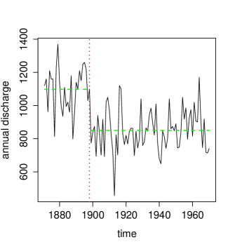
Figure 1. Measurements of the annual discharge of the river Nile at Aswan in $10^{8}$ $m^{3}$ for the years 1871-1970. The dotted line indicates the location of the change-point; the dashed lines designate the sample means for the pre-break and post-break samples.

The plot in Figure 1 depicts the annual volume of discharge from the Nile river at Aswan in $10^{8}$ $m^{3}$ for the years 1871 to 1970. The data set has been analyzed for the detection of a change-point by numerous authors under differing assumptions concerning the data generating random process and by usage of diverse methods. Amongst others, Cobb [19], MacNeill, Tang and Jandhyala [41], Wu and Zhao [57] and Shao [48] provided statistically significant evidence for a decrease of the Nile’s annual discharge towards the end of the 19th century. The construction of the Aswan Low Dam between 1898 and 1902 serves as a popular explanation for an abrupt change in the data.

The value of the self-normalized Wilcoxon test statistic computed with respect to the data is given by $T_{n}(\tau_{1},\tau_{2})=13.48729$. For a level of significance of $5\%$, the self-normalized Wilcoxon change-point test rejects the hypothesis for every possible value of $H\in\left(\frac{1}{2},1\right)$. Furthermore, we approximate the distribution of the self-normalized Wilcoxon test statistic by the sampling window method with block size $l=\lfloor\sqrt{n}\rfloor=10$. The subsampling-based test decision also indicates the existence of a change-point in the mean of the data, even if we consider the $99\%$-quantile of $\hat{F}_{l,n}$.

In particular, previous analysis of the Nile data done by Wu and Zhao [57] and Balke [7] suggests that the change in the discharge volume occurred in 1899. We applied the self-normalized Wilcoxon test and the sampling window method to the corresponding pre-break and post-break samples. Neither of these two approaches leads to rejection of the hypothesis, so that it seems reasonable to consider both samples as stationary. At this point, it is interesting to note that, based on the whole sample, local Whittle estimation with bandwidth parameter $m=\lfloor n^{2/3}\rfloor$ suggests the existence of long range dependence characterized by an Hurst parameter $\hat{H}=0.962$, whereas the estimates for the pre-break and post-break samples given by $\hat{H}_{1}=0.517$ and $\hat{H}_{2}=0.5$, respectively, should be considered as indication of short range dependent data. In this regard, our findings support the conjecture of spurious long memory caused by a change-point and therefore coincide with the results of Shao [48].

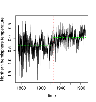
Figure 2. Monthly temperature of the northern hemisphere for the years 1854-1989 from the data base held at the Climate Research Unit of the University of East Anglia, Norwich, England. The temperature anomalies (in degrees C) are calculated with respect to the reference period 1950-1979. The dotted line indicates the location of the potential change-point; the dashed lines designate the sample means for the pre-break and post-break samples.

The second data set consists of the seasonally adjusted monthly deviations of the temperature (degrees C) for the northern hemisphere during the years 1854 to 1989 from the monthly averages over the period 1950 to 1979. The data results from spatial averaging of temperatures measured over land and sea. At first sight, the plot in Figure 2 may suggest an increasing trend as well as an abrupt change of the temperature deviations. Statistical evidence for a positive deterministic trend implies affirmation of the conjecture that there has been global warming during the last decades.

In scientific discourse, the question of whether the Northern hemisphere temperature data acts as an indicator for global warming of the atmosphere is a controversial issue. Deo and Hurvich [24] provided some indication for global warming by fitting a linear trend to the data. Beran and Feng [8] considered a more general stochastic model by the assumption of so-called semiparametric fractional autoregressive (SEMIFAR) processes. Their method did not deliver sufficient statistical evidence for a deterministic trend. Wang [55] applied another method for the detection of gradual change to the global temperature data and did not detect an increasing trend , either. Nonetheless, he offers an alternative explanation for the occurrence of a trend-like behavior by pointing out that it may have been generated by stationary long range dependent processes. In contrast, it is shown in Shao [48] that the existence of a change-point in the mean yields yet another explanation for the performance of the data.

The value of the self-normalized Wilcoxon test statistic computed with respect to the data is given by $T_{n}(\tau_{1},\tau_{2})=18.98636$. Consequently, the self-normalized Wilcoxon change-point test would reject the hypothesis for every possible value of $H\in\left(\frac{1}{2},1\right)$ at a level of significance of $1\%$. In addition, an application of the sampling window method with respect to the self-normalized Wilcoxon test statistic based on comparison of $T_{n}(\tau_{1},\tau_{2})$ with the $99\%$-quantile of the sampling distribution $\hat{F}_{l,n}$ yields a test decision in favor of the alternative hypothesis for any choice of the block length $l\in\{\lfloor n^{\gamma}\rfloor|\ \gamma=0.3,0.4,\ldots,0.9\}=\{9,19,40,84,177,371,778\}$. All in all, both testing procedures provide strong evidence for the existence of a change in the mean.

According to Shao [48] the change-point is located around October 1924. Based on the whole sample local Whittle estimation with bandwidth $m=\lfloor n^{2/3}\rfloor$ provides an estimator $\hat{H}=0.811$. The estimated Hurst parameters for the pre-break and post-break sample are $\hat{H}_{1}=0.597$ and $\hat{H}_{2}=0.88$, respectively. Neither of both testing procedures, i.e. subsampling with respect to the self-normalized Wilcoxon test statistic and comparison of the value of $T_{n}(\tau_{1},\tau_{2})$ with the corresponding critical values of its limit distribution, provides evidence for another change-point in the pre-break or post-break sample.

Moreover, computation of the test statistic that allows for two change-point locations yields $T_{n}(\tau_{1},\tau_{2},\varepsilon)=17.88404$ (for $\tau_{1}=1-\tau_{2}=\varepsilon=0.15$), i.e. if compared to the values in Table 1, the test statistic only surpasses the critical value corresponding to $H=0.501$ and a significance level of $10\%$, but does not exceed any of the other values. Subsampling with respect to the test statistic $T_{n}(\tau_{1},\tau_{2},\varepsilon)$ does not support the conjecture of two changes, either. In fact, subsampling leads to a rejection of the hypothesis when the block length equals $l=\lfloor n^{0.7}\rfloor=177$ (based on a comparison of $T_{n}(\tau_{1},\tau_{2},\varepsilon)$ with the $95\%$-quantile of the corresponding sampling distribution $\hat{F}_{l,n}$), but yields a test decision in favor of the hypothesis for block lengths $l\in\{\lfloor n^{\gamma}\rfloor|\ \gamma=0.5,0.6,0.8,0.9\}=\{40,84,371,778\}$ and for comparison with the $90\%$-quantile of $\hat{F}_{l,n}$.

Therefore, it seems safe to conclude that the appearance of long memory in the post-break sample is not caused by another change-point in the mean. The pronounced difference between the local Whittle estimators $\hat{H}_{1}$ and $\hat{H}_{2}$ suggests a change in the dependence structure of the times series. Another explanation might be a gradual change of the temperature in the post-break period. We conjecture that our test has only low power in the case of a gradual change, because the denominator of our self-normalized test statistic is inflated as the ranks systematically deviate from the mean rank of the first and second part. When using subsampling, the trend also appears in subsamples so that we fail to approximate the distribution under the hypothesis.

As pointed out by one of the referees, the Northern hemisphere temperature data does not seem to be second-order stationary; the variance in the first part of the time series seems to be higher. Such a change in variance should also result in a loss of power. The reason is that the ranks in the part with the higher variance are more extreme, so that the distance to the mean rank of this part is larger. This leads to a higher value of the denominator of our self-normalized test statistic and consequently to a lower value of the ratio.

The third data set consists of the arrival rate of Ethernet data (bytes per 10 milliseconds) from a local area network (LAN) measured at Bellcore Research and Engineering Center in 1989. For more information on the LAN traffic monitoring we refer to Leland and Wilson [38] and Beran [9]. Figure 3 reveals that the observations are strongly right-skewed. As the self-normalized Wilcoxon test is based on ranks, we do not expect that this will affect our analysis.

Figure 3. Ethernet traffic in bytes per 10 milliseconds from a LAN measured at Bellcore Research Engineering Center.

Coulon, Chabert and Swami [20] examined this data set for change-points before. The method proposed in their paper is based on the assumption that a FARIMA model holds for segments of the data. The number of different sections and the location of the change-points are chosen by a model selection criterion. The algorithm proposed by Coulon et al. [20] detects multiple changes in the parameters of the corresponding FARIMA time series.

In contrast, an application of the self-normalized Wilcoxon change-point test does not provide evidence for a change-point in the mean: the value of the test statistic is given by $T_{n}(\tau_{1},\tau_{2})=3.270726$, i.e. even for a level of significance of 10%, the self-normalized Wilcoxon change-point test does not reject the hypothesis for any value $H\in\left(\frac{1}{2},1\right)$. Furthermore, subsampling with respect to the self-normalized Wilcoxon test statistic does not lead to a rejection of the hypothesis , either (for any choice of block length $l\in\{\lfloor n^{\gamma}\rfloor|\ \gamma=0.3,0.4,\ldots,0.9\}=\{12,27,63,144,332,761,1745\}$ and for comparison with the $90\%$-quantile of the corresponding sampling distribution $\hat{F}_{l,n}$).

Taking into consideration that the data set contains ties (the value $0$ appears several times), we also applied the self-normalized Wilcoxon test statistic based on the modified ranks $\tilde{R}_{i}$ and used subsampling with respect to this statistic. Both approaches did not lead to a rejection of the hypothesis.

An application of the test statistic constructed for the detection of two changes yields a value of $T_{n}(\tau_{1},\tau_{2},\varepsilon)=15.24527$ when $\varepsilon=\tau_{1}=1-\tau_{2}=0.15$. Clearly, this does not lead to a rejection of the hypothesis for any value of the parameter $H$. In addition, subsampling based on comparison of $T_{n}(\tau_{1},\tau_{2},\varepsilon)$ with the $90\%$-quantile of the corresponding sampling distribution $\hat{F}_{l,n}$ does not provide evidence for the assertion of multiple changes for any block lenght $l\in\{\lfloor n^{\gamma}\rfloor|\ \gamma=0.5,0.6,0.7,0.8\}=\{63,144,332,761\}$ in the data, either.

These results do not coincide with the analysis of the previous authors. On the one hand this may be due to the fact that the applied methods differ considerably from the testing procedures applied before. On the other hand, the change-point estimation algorithm proposed in Coulon, Chabert and Swami [20] is not robust to skewness or heavy-tailed distributions and decisively relies on the assumption of FARIMA time series. However, this seems to contradict observations made by Bhansali and Kokoszka [14] as well as Taqqu and Teverovsky [54] who stress that the model that fits the Ethernet traffic data is very unlikely to be FARIMA.

Estimation of the Hurst parameter by the local Whittle procedure with bandwidth parameter $m=\lfloor n^{2/3}\rfloor$ yields an estimate of $\hat{H}=0.845$ and therefore indicates the existence of long range dependence. This is consistent with the results of Leland et al. [37] and Taqqu and Teverovsky [54].

In the three data examples, we find that the results obtained by subsampling and by parameter estimation are in good accordance with each other. The methods take into account long range dependence or heavy tails, but still detect a change in location in the first two examples. For the third data example our analysis supports the hypothesis of stationarity.

4. Simulations

We will now investigate the finite sample performance of the subsampling procedure with respect to the self-normalized Wilcoxon test and with respect to the classical Wilcoxon change-point test. Moreover, we will compare these results to the performance of the tests when the test decision is based on critical values obtained from the asymptotic distribution of the test statistic.

For this purpose, we consider subordinated Gaussian time series $\left(X_{n}\right)_{n\in\mathbb{N}}$, $X_{n}=G(\xi_{n})$, where $\left(\xi_{n}\right)_{n\in\mathbb{N}}$ is fractional Gaussian noise (introduced in Examples 1 and 2) with Hurst parameter $H\in\{0.6,0.7,0.8,0.9\}$ and covariance function

$$\gamma(k)\sim k^{-D}\left(1-\frac{D}{2}\right)\left(1-D\right),$$

where $D=2-2H$. Initially, we take $G(t)=t$, so that $\left(X_{n}\right)_{n\in\mathbb{N}}$ has normal marginal distributions. We also consider the transformation

$$G(t)=\left(\frac{\beta k^{2}}{(\beta-1)^{2}(\beta-2)}\right)^{-\frac{1}{2}}\left(k(\Phi(t))^{-\frac{1}{\beta}}-\frac{\beta k}{\beta-1}\right)$$

(with $\Phi$ denoting the standard normal distribution function) so as to generate Pareto-distributed data with parameters $k,\beta>0$ (referred to as Pareto($\beta$, $k$)). In both cases, the Hermite rank $r$ of $1_{\left\{G(\xi_{i})\leq x\right\}}-F(x),x\in\mathbb{R}$, equals $r=1$ and

$$\left|\int_{\mathbb{R}}J_{1}(x)dF(x)\right|=\frac{1}{2\sqrt{\pi}};$$

see [22].

Under the above conditions, the critical values of the asymptotic distribution of the self-normalized Wilcoxon test statistic are reported in Table 2 in [12]. The limit of the Wilcoxon change-point test statistic can be found in [22], the corresponding critical values can be taken from Table 1 in [12].

The frequencies of rejections of both testing procedures are reported in Table 2 and Table 3 for the self-normalized Wilcoxon change-point test and in Table 4 and Table 5 for the classical Wilcoxon test (without self-normalization). The calculations are based on $5,000$ realizations of time series with sample size $n=300$ and $n=500$. We have chosen block lengths $l=l_{n}=\lfloor n^{\gamma}\rfloor$ with $\gamma\in\left\{0.4,0.5,0.6\right\}$. As level of significance we chose $5\%$, i.e. we compare the values of the test statistic with the corresponding critical values of its asymptotic distribution and the corresponding quantile of the empirical distribution function $\hat{F}_{l,n}$, respectively.

For the usual testing procedures the estimation of the Hermite rank $r$, the slowly varying function $L_{\gamma}$ and the integral $\int J_{1}(x)dF(x)$ is neglected. Yet, for every simulated time series we estimate the Hurst parameter $H$ by the local Whittle estimator $\hat{H}$ proposed in Künsch [35]. This estimator is based on an approximation of the spectral density by the periodogram at the Fourier frequencies. It depends on the spectral bandwidth parameter $m=m(n)$ which denotes the number of Fourier frequencies used for the estimation. If the bandwidth $m$ satisfies $\frac{1}{m}+\frac{m}{n}\longrightarrow 0$ as $n\longrightarrow\infty$, the local Whittle estimator is a consistent estimator for $H$; see Robinson [47]. For convenience we always choose $m=\lfloor n^{2/3}\rfloor$ in this article. The critical values corresponding to the estimated values of $H$ are determined by linear interpolation.

Under the alternative $\operatorname{\mathbf{A}}$ we analyze the power of the testing procedures (the frequency of rejection) by considering different choices for the height of the level shift (denoted by $h$) and the location $[n\tau]$ of the change-point. In the tables the columns that are superscribed by “$h=0$” correspond to the frequency of a type 1 error, i.e. the rejection rate under the hypothesis $\operatorname{\mathbf{H}}$.

For the self-normalized Wilcoxon change-point test (based on the asymptotic distribution), the empirical size almost equals the level of significance of $5\%$ for normally distributed data (see Table 2). The sampling window method yields rejection rates that slightly exceed this level. For Pareto($3$, $1$) time series both testing procedures lead to similar results and tend to reject the hypothesis too often when there is no change. With regard to the empirical power, it is notable that for fractional Gaussian noise time series the sampling window method yields considerably better power than the test based on asymptotic critical values. If Pareto($3$, $1$)-distributed time series are considered, the empirical power of the subsampling procedure is still better than the empirical power that results from using asymptotic critical values. However, in this case, the deviation of the rejection rates is rather small. While the empirical size is not much affected by the Hurst parameter $H$, the empirical power is lower for $H=0.8,0.9$.

Considering the classical Wilcoxon test (without self-normalization), it is notable that for both procedures the empirical size is in most cases not close to the nominal level of significance ($5\%$), ranging from $1.1\%$ to $20.8\%$ using subsampling and from $2.6\%$ to $36.0\%$ using asymptotic critical values. In general, the sampling window method becomes more conservative for higher values of the Hurst parameter $H$, while the test based on the asymptotic distribution becomes more liberal. Under the alternative, the usual application of the Wilcoxon test yields better power than the sampling window method, especially for high values of $H$. It should be emphasized that this comparison is problematic because the rejection frequencies under the hypothesis differ.

We conclude that the self-normalized Wilcoxon change-point test is more reliable than the classical change-point test. The reason might be that in the scaling of the classical test, the estimator $\hat{H}$ of the Hurst parameter enters as a power of the sample size $n$. Thus, a small error in this estimation might lead to a large error in the value of the test statistic. By using the sampling window method for the self-normalized version, we avoid the estimation of unknown parameters so that the performance is similar to the performance of the classical testing procedure which compares the values of the test statistic with the corresponding critical values.

Note that in most cases covered by our simulations the choice of the block length for the subsampling procedure does not have a big impact on the frequency of a type 1 error. Considering the self-normalized Wilcoxon change-point test, an increase of the block length tends to go along with a decrease in power, especially for big values of the Hurst parameter $H$ and Pareto-distributed random variables. For smaller values of $H$ the effect is not pronounced. We recommend using a block length $\lfloor n^{0.4}\rfloor$ or $\lfloor n^{0.5}\rfloor$ for the self-normalized change-point test as the choice $l=\lfloor n^{0.6}\rfloor$ implies worse properties in most cases.

An application of the subsampling testing procedure to the classical (non-self-normalized) Wilcoxon test for different choices of the block length shows the opposite effect on the rejection rate under the alternative: an increase of the block length results in a higher frequency of rejections. Here, the block length $\lfloor n^{0.6}\rfloor$ leads to better results in many cases. However, we recommend to not use this test, but to self-normalize the test statistic instead.

An alternative way of choosing the block length would be to apply the data-driven block selection rule proposed by Götze and Rac̆kauskas [27] and Bickel and Sakov [15]. Although the algorithm had originally been implemented for applications of the $m$-out-of-$n$ bootstrap to independent and identically distributed data, it also lead to satisfactory simulation results in applications to long range dependent time series (see [33]). Another general approach to the selection of the block size in the context of hypothesis testing is given by Algorithm 9.4.2 in Politis, Romano and Wolf [46].

Table 2. Rejection rates of the self-normalized Wilcoxon change-point test obtained by subsampling (left) with block length $l=\lfloor n^{\gamma}\rfloor$, $\gamma\in\left\{0.4,0.5,0.6\right\}$, and by comparison with asymptotic critical values (right) for fractional Gaussian noise of length $n$ with Hurst parameter $H$.

			sampling window method										asymptotic distribution
							$\tau=0.25$			$\tau=0.5$					$\tau=0.25$			$\tau=0.5$
fGn	$n$		$l$		$h=0$		$h=0.5$	$h=1$		$h=0.5$	$h=1$		$h=0$		$h=0.5$	$h=1$		$h=0.5$	$h=1$
$H=0.6$	300		9		0.041		0.263	0.700		0.502	0.952
			17		0.064		0.313	0.742		0.570	0.964		0.044		0.209	0.521		0.424	0.861
			30		0.070		0.322	0.705		0.555	0.943
	500		12		0.053		0.396	0.859		0.697	0.994
			22		0.060		0.421	0.861		0.720	0.995		0.049		0.303	0.687		0.577	0.958
			41		0.069		0.411	0.829		0.697	0.991
$H=0.7$	300		9		0.057		0.155	0.412		0.291	0.759
			17		0.070		0.171	0.423		0.313	0.763		0.053		0.108	0.268		0.228	0.611
			30		0.077		0.177	0.403		0.314	0.737
	500		12		0.056		0.183	0.513		0.382	0.856
			22		0.059		0.193	0.508		0.382	0.854		0.048		0.133	0.359		0.302	0.730
			41		0.065		0.192	0.476		0.387	0.819
$H=0.8$	300		9		0.070		0.126	0.251		0.223	0.526
			17		0.067		0.117	0.234		0.208	0.494		0.048		0.081	0.144		0.141	0.362
			30		0.073		0.114	0.218		0.201	0.466
	500		12		0.066		0.121	0.295		0.217	0.591
			22		0.068		0.114	0.278		0.210	0.567		0.053		0.085	0.198		0.163	0.462
			41		0.069		0.119	0.257		0.205	0.532
$H=0.9$	300		9		0.093		0.126	0.208		0.209	0.462
			17		0.074		0.097	0.161		0.169	0.397		0.057		0.065	0.106		0.125	0.308
			30		0.073		0.095	0.145		0.165	0.367
	500		12		0.079		0.105	0.194		0.185	0.461
			22		0.067		0.091	0.166		0.162	0.416		0.051		0.068	0.120		0.128	0.350
			41		0.063		0.087	0.146		0.152	0.391

Table 3. Rejection rates of the self-normalized Wilcoxon change-point test obtained by subsampling (left) with block length $l=\lfloor n^{\gamma}\rfloor$, $\gamma\in\left\{0.4,0.5,0.6\right\}$, and by comparison with asymptotic critical values (right) for Pareto($3$, $1$)-transformed fractional Gaussian noise of length $n$ with Hurst parameter $H$.

			sampling window method										asymptotic distribution
							$\tau=0.25$			$\tau=0.5$					$\tau=0.25$			$\tau=0.5$
Pareto(3, 1)	$n$		$l$		$h=0$		$h=0.5$	$h=1$		$h=0.5$	$h=1$		$h=0$		$h=0.5$	$h=1$		$h=0.5$	$h=1$
$H=0.6$	300		9		0.041		0.847	0.977		0.990	1.000
			17		0.067		0.871	0.946		0.990	1.000		0.056		0.820	0.912		0.984	0.999
			30		0.070		0.831	0.946		0.979	1.000
	500		12		0.055		0.947	0.997		0.999	1.000
			22		0.066		0.946	0.994		0.999	1.000		0.061		0.920	0.970		0.996	1.000
			41		0.071		0.921	0.976		0.996	1.000
$H=0.7$	300		9		0.057		0.571	0.821		0.990	0.994
			17		0.064		0.527	0.738		0.876	0.990		0.070		0.529	0.702		0.856	0.982
			30		0.077		0.527	0.738		0.842	0.975
	500		12		0.066		0.693	0.904		0.949	0.999
			22		0.068		0.684	0.893		0.942	0.998		0.076		0.663	0.820		0.940	0.995
			41		0.072		0.632	0.838		0.921	0.994
$H=0.8$	300		9		0.070		0.355	0.574		0.703	0.931
			17		0.068		0.284	0.454		0.666	0.905		0.072		0.297	0.428		0.640	0.875
			30		0.073		0.284	0.454		0.633	0.857
	500		12		0.064		0.401	0.609		0.738	0.948
			22		0.063		0.379	0.581		0.714	0.933		0.069		0.369	0.510		0.715	0.920
			41		0.064		0.345	0.509		0.688	0.903
$H=0.9$	300		9		0.093		0.253	0.396		0.597	0.832
			17		0.071		0.168	0.254		0.532	0.772		0.073		0.165	0.236		0.499	0.738
			30		0.073		0.168	0.254		0.482	0.729
	500		12		0.073		0.256	0.405		0.585	0.839
			22		0.064		0.219	0.340		0.547	0.802		0.068		0.199	0.296		0.529	0.782
			41		0.065		0.190	0.296		0.503	0.762

Table 4. Rejection rates of the classical Wilcoxon change-point test obtained by subsampling (left) with block length $l=\lfloor n^{\gamma}\rfloor$, $\gamma\in\left\{0.4,0.5,0.6\right\}$, and by comparison with asymptotic critical values (right) for fractional Gaussian noise of length $n$ with Hurst parameter $H$.

			sampling window method										asymptotic distribution
							$\tau=0.25$			$\tau=0.5$					$\tau=0.25$			$\tau=0.5$
fGn	$n$		$l$		$h=0$		$h=0.5$	$h=1$		$h=0.5$	$h=1$		$h=0$		$h=0.5$	$h=1$		$h=0.5$	$h=1$
$H=0.6$	300		9		0.066		0.20	0.232		0.386	0.591
			17		0.054		0.223	0.411		0.439	0.784		0.026		0.096	0.160		0.223	0.727
			30		0.059		0.264	0.529		0.663	0.870
	500		12		0.063		0.285	0.436		0.569	0.856
			22		0.058		0.345	0.663		0.627	0.952		0.036		0.148	0.256		0.378	0.897
			41		0.062		0.397	0.789		0.683	0.975
$H=0.7$	300		9		0.052		0.080	0.088		0.162	0.302
			17		0.049		0.095	0.158		0.206	0.466		0.035		0.067	0.228		0.167	0.665
			30		0.051		0.120	0.227		0.267	0.593
	500		12		0.042		0.104	0.153		0.249	0.539
			22		0.039		0.131	0.267		0.287	0.689		0.030		0.079	0.259		0.225	0.714
			41		0.046		0.160	0.373		0.343	0.789
$H=0.8$	300		9		0.028		0.030	0.031		0.054	0.092
			17		0.029		0.038	0.048		0.075	0.179		0.077		0.153	0.421		0.245	0.673
			30		0.034		0.057	0.088		0.070	0.272
	500		12		0.023		0.031	0.036		0.064	0.162
			22		0.028		0.044	0.070		0.097	0.273		0.050		0.112	0.439		0.226	0.714
			41		0.039		0.071	0.129		0.137	0.391
$H=0.9$	300		9		0.009		0.010	0.006		0.016	0.020
			17		0.009		0.014	0.009		0.021	0.060		0.36		0.484	0.739		0.524	0.830
			30		0.015		0.029	0.028		0.011	0.153
	500		12		0.008		0.006	0.003		0.015	0.026
			22		0.011		0.009	0.011		0.029	0.086		0.319		0.439	0.743		0.511	0.845
			41		0.021		0.021	0.032		0.058	0.197

Table 5. Rejection rates of the classical Wilcoxon change-point test obtained by subsampling (left) with block length $l=\lfloor n^{\gamma}\rfloor$, $\gamma\in\left\{0.4,0.5,0.6\right\}$, and by comparison with asymptotic critical values (right) for Pareto($3$, $1$)-transformed fractional Gaussian noise of length $n$ with Hurst parameter $H$.

			sampling window method										asymptotic distribution
							$\tau=0.25$			$\tau=0.5$					$\tau=0.25$			$\tau=0.5$
Pareto(3, 1)	$n$		$l$		$h=0$		$h=0.5$	$h=1$		$h=0.5$	$h=1$		$h=0$		$h=0.5$	$h=1$		$h=0.5$	$h=1$
$H=0.6$	300		9		0.170		0.949	0.742		0.991	0.923
			17		0.130		0.963	0.861		0.996	0.991		0.108		0.938	0.985		0.998	1.000
			30		0.109		0.962	0.871		0.998	0.998
	500		12		0.163		0.991	0.916		1.000	0.993
			22		0.132		0.997	0.976		1.000	0.999		0.128		0.988	0.999		1.000	1.000
			41		0.114		0.997	0.989		1.000	1.000
$H=0.7$	300		9		0.224		0.785	0.568		0.939	0.796
			17		0.175		0.802	0.680		0.955	0.949		0.179		0.833	0.969		0.974	0.999
			30		0.140		0.789	0.708		0.959	0.976
	500		12		0.208		0.921	0.763		0.989	0.956
			22		0.167		0.931	0.862		0.992	0.996		0.191		0.940	0.994		0.996	1.000
			41		0.143		0.925	0.891		0.994	0.998
$H=0.8$	300		9		0.203		0.508	0.326		0.743	0.565
			17		0.160		0.496	0.347		0.776	0.808		0.204		0.729	0.925		0.918	0.993
			30		0.137		0.484	0.364		0.791	0.881
	500		12		0.190		0.639	0.445		0.865	0.770
			22		0.160		0.649	0.513		0.886	0.929		0.212		0.805	0.963		0.948	0.999
			41		0.137		0.626	0.556		0.890	0.961
$H=0.9$	300		9		0.128		0.150	0.077		0.320	0.336
			17		0.097		0.128	0.071		0.403	0.550		0.309		0.712	0.901		0.848	0.966
			30		0.092		0.125	0.077		0.481	0.677
	500		12		0.112		0.159	0.089		0.402	0.436
			22		0.100		0.161	0.101		0.518	0.680		0.27		0.726	0.911		0.851	0.975
			41		0.095		0.170	0.106		0.571	0.771

5. Proofs

5.1. Auxiliary Results

Lemma 1.

Under Assumption 2, there is a constant $K_{D}<\infty$, such that for all $x_{1},\ldots,x_{l}\in{\mathds{R}}$ with ${\rm Var}(\sum_{i=1}^{l}x_{i}\xi_{i})=1$

$$\sum_{i=1}^{l}x_{i}^{2}\leq K_{D}.$$

Proof.

Recall that we can rewrite the covariances as

$$\gamma(k)=\int_{-\pi}^{\pi}\operatorname{e}^{ik\lambda}f(\lambda)d\lambda$$

and that the spectral density $f$ can be written as $f(\lambda)=L_{f}(|\lambda|)|\lambda|^{D-1}$. By our assumptions $L_{f}(x)\geq C_{\text{min}}$ for a constant $C_{\text{min}}>0$, so that we can conclude that

$$1= {\rm Var}\Big{(}\sum_{i=1}^{l}x_{i}\xi_{i}\Big{)}=\sum\limits_{1\leq j,k\leq l}x_{j}x_{k}\gamma(j-k)$$

$$= \sum\limits_{1\leq j,k\leq l}x_{j}x_{k}\int_{-\pi}^{\pi}\operatorname{e}^{i(j-k)\lambda}f(\lambda)d\lambda=\sum\limits_{1\leq j,k\leq l}x_{j}x_{k}\int_{-\pi}^{\pi}\operatorname{e}^{i(j-k)\lambda}L_{f}(|\lambda|)|\lambda|^{D-1}d\lambda$$

$$= 2\int_{0}^{\pi}\!\sum\limits_{1\leq j,k\leq l}x_{j}x_{k}\operatorname{e}^{i(j-k)\lambda}L_{f}(\lambda)\lambda^{D-1}d\lambda=2\int_{0}^{\pi}\bigg{|}\sum\limits_{j=1}^{l}x_{j}\operatorname{e}^{-ij\lambda}\bigg{|}^{2}L_{f}(\lambda)\lambda^{D-1}d\lambda$$

$$\geq 2C_{\text{min}}\pi^{D-1}\int_{0}^{\pi}\bigg{|}\sum\limits_{j=1}^{l}x_{j}\operatorname{e}^{-ij\lambda}\bigg{|}^{2}d\lambda.$$

We rewrite the integrand as

$$\bigg{|}\sum\limits_{j=1}^{l}x_{j}\operatorname{e}^{-ij\lambda}\bigg{|}^{2} =\sum\limits_{1\leq j,k\leq l}x_{j}x_{k}\operatorname{e}^{-ij\lambda}\operatorname{e}^{ik\lambda}=\sum\limits_{j=1}^{l}x_{j}^{2}+\sum\limits_{j\neq k}x_{j}x_{k}\operatorname{e}^{-i(j-k)\lambda}$$

$$=\sum\limits_{j=1}^{l}x_{j}^{2}+\sum\limits_{j<k}x_{j}x_{k}\left(\operatorname{e}^{-i(j-k)\lambda}+\operatorname{e}^{-i(k-j)\lambda}\right)$$

$$=\sum\limits_{j=1}^{l}x_{j}^{2}+2\sum\limits_{j<k}x_{j}x_{k}\cos((k-j)\lambda)=\sum\limits_{1\leq j,k\leq l}x_{j}x_{k}\cos((k-j)\lambda).$$

As a result, we have

$$\int_{0}^{\pi}\bigg{|}\sum\limits_{j=1}^{l}x_{j}\operatorname{e}^{-ij\lambda}\bigg{|}^{2}d\lambda =\int_{0}^{\pi}\sum\limits_{1\leq j,k\leq l}x_{j}x_{k}\cos((k-j)\lambda)d\lambda$$

$$=\sum\limits_{1\leq j,k\leq l}x_{j}x_{k}\int_{0}^{\pi}\cos((k-j)\lambda)d\lambda$$

$$=\sum\limits_{j=1}^{l}x_{j}^{2}\int_{0}^{\pi}\cos(0)d\lambda+\sum\limits_{j\neq k}x_{j}x_{k}\int_{0}^{\pi}\cos((k-j)\lambda)d\lambda$$

$$=\pi\sum\limits_{j=1}^{l}x_{j}^{2}.$$

All in all, this yields

$$1={\rm Var}\left(\sum_{i=1}^{l}x_{i}\xi_{i}\right)\geq 2C_{\text{min}}\pi^{D-1}\int_{0}^{\pi}\bigg{|}\sum\limits_{j=1}^{l}x_{j}\operatorname{e}^{-ij\lambda}\bigg{|}^{2}d\lambda=2C_{\text{min}}\pi^{D}\sum\limits_{j=1}^{l}x_{j}^{2}.$$

Therefore, the statement of the lemma holds with $K_{D}=1/(2C_{\text{min}}\pi^{D})$.

∎

Lemma 2.

Under Assumption 2, there are constants $K^{\prime}_{D}<\infty$ and $l_{0}\in{\mathds{N}}$ such that

$$\bigg{|}\sum_{i=1}^{l}x_{i}\bigg{|}\leq K^{\prime}_{D}l^{D/2}$$

for all $l\geq l_{0}$ and $x_{1},\ldots,x_{l}\in{\mathds{R}}$ with ${\rm Var}\left(\sum_{i=1}^{l}x_{i}\xi_{i}\right)=1$.

Proof.

The statement of the proof is equivalent to the existence of a constant $C>0$, such that for all $x_{1},\ldots,x_{l}\in{\mathds{R}}$ with $\sum_{i=1}^{l}x_{i}=1$, we have

$${\rm Var}\left(\sum_{i=1}^{l}x_{i}\xi_{i}\right)\geq Cl^{-D}.$$

Let $x_{1}^{\star},\ldots,x_{l}^{\star}\in{\mathds{R}}$ with $\sum_{i=1}^{l}x_{i}^{\star}=1$ be the values that minimize ${\rm Var}\left(\sum_{i=1}^{l}x_{i}^{\star}\xi_{i}\right)$. Then $\hat{\mu}_{\xi}(\xi_{1},\ldots,\xi_{n}):=\sum_{i=1}^{l}x_{i}^{\star}\xi_{i}$ is the best linear unbiased estimator for $\mu:=E(\xi_{1})$. For a process $(\zeta_{n})_{n\in{\mathds{N}}}$ with spectral density

$$f_{\zeta}(x)=\frac{1}{2\pi}\left|1-e^{ix}\right|^{D-1},$$

we have

$${\rm Var}\left(\hat{\mu}_{\zeta}(\zeta_{1},\ldots,\zeta_{n})\right)\geq C_{1}l^{-D}$$

for a constant $C_{1}>0$ by a Corollary of Adenstedt [1] (see p. 1101). We rewrite the spectral density $f_{\zeta}$ of $(\zeta_{n})_{n\in{\mathds{N}}}$ with the help of the spectral density $f$ of $(\xi_{n})_{n\in{\mathds{N}}}$ as

$$f_{\zeta}(x)=f(x)\frac{\left|1-e^{ix}\right|^{D-1}}{2\pi|x|^{D-1}L_{f}(x)}.$$

Note that the function $g$ with $g(x)=\frac{\left|1-e^{ix}\right|^{D-1}}{2\pi|x|^{D-1}L_{f}(x)}$ is bounded, as we assumed that $L_{f}$ is bounded away from $0$. Hence, we have

$${\rm Var}\left(\hat{\mu}_{\xi}(\xi_{1},\ldots,\xi_{n})\right)\geq\frac{1}{g(0)}{\rm Var}\left(\hat{\mu}_{\zeta}(\zeta_{1},\ldots,\zeta_{n})\right)\geq Cl^{-D}$$

for all $l\geq l_{0}$ by Lemma 4.4 in [1]. ∎

The next Lemma deals with the $\rho$-mixing coefficient, which is defined in the following way: Let $\mathcal{A},\mathcal{B}$ be two $\sigma$-fields. Then

$$\rho(\mathcal{A},\mathcal{B}):=\sup{\rm corr}(X,Y),$$

where the supremum is taken over all $\mathcal{A}$-measurable random variables $X$ and all $\mathcal{B}$-measurable random variables $Y$. For details we recommend the book of Bradley [18].

Lemma 3.

Under Assumption 2, there are constants $C_{1},C_{2}<\infty$ such that

$$\rho(k,l):=\rho\big{(}\sigma(\xi_{i},1\leq i\leq l),\sigma(\xi_{j},k+l+1\leq j\leq k+2l)\big{)}\\ \leq C_{1}\left(k/l\right)^{-D}L_{\gamma}(k)+C_{2}l^{2}k^{-D-1}\max\{L_{\gamma}(k),1\}$$

for all $k\in{\mathds{N}}$ and all $l\in\{l_{k},\ldots,k\}$.

Proof.

Kolmogorov and Rozanov [34] proved that there exist real numbers $a_{1},a_{2},\ldots,a_{l}$, $b_{1},b_{2},\ldots,b_{l}$ such that

$$\rho\big{(}\sigma(\xi_{i},1\leq i\leq l),\sigma(\xi_{j},k+l+1\leq j\leq k+2l)\big{)}={\rm Cov}\Big{(}\sum\limits_{i=1}^{l}a_{i}\xi_{i},\sum\limits_{j=1}^{l}b_{j}\xi_{k+l+j}\Big{)}$$

and ${\rm Var}\big{(}\sum_{i=1}^{l}a_{i}\xi_{i}\big{)}={\rm Var}\big{(}\sum_{j=1}^{l}b_{j}\xi_{k+l+j}\big{)}=1$. The triangular inequality yields

$$\bigg{|}{\rm Cov}\Big{(}\sum\limits_{i=1}^{l}a_{i}\xi_{i},\sum_{j=1}^{l}b_{j}\xi_{k+l+j}\Big{)}\bigg{|}\\ \leq\Big{|}\sum\limits_{i=1}^{l}a_{i}\sum\limits_{j=1}^{l}b_{j}\Big{|}\left|\gamma(k)\right|+\sum\limits_{i=1}^{l}\sum_{j=1}^{l}|a_{i}||b_{j}|\left|\gamma(k)-\gamma(k+l+j-i)\right|.$$

We will treat the two summands on the right hand side separately. For the first term, it follows by Lemma 2 that

$$\Big{|}\sum\limits_{i=1}^{l}a_{i}\sum_{j=1}^{l}b_{j}\Big{|}\left|\gamma(k)\right|=\Big{|}\sum\limits_{i=1}^{l}a_{i}\Big{|}\Big{|}\sum_{j=1}^{l}b_{j}\Big{|}\left|\gamma(k)\right|\leq K^{\prime 2}_{d}l^{D}L_{\gamma}(k)k^{-D}.$$

Before we deal with the second summand, we observe that by Hölder’s inequality and Lemma 1

$$\sum\limits_{i=1}^{l}|a_{i}|\leq\sqrt{l\sum\limits_{i=1}^{l}a_{i}^{2}}\leq\sqrt{K_{D}}\sqrt{l}\ \ \text{and}\ \ \sum\limits_{j=1}^{l}|b_{j}|\leq\sqrt{l\sum\limits_{j=1}^{l}b_{j}^{2}}\leq\sqrt{K_{D}}\sqrt{l}.$$

Due to Assumption 2

$$\sup\limits_{|k-\tilde{k}|\leq 2l-1}\left|L_{\gamma}(k)-L_{\gamma}(\tilde{k})\right|\leq K\frac{l}{k}$$

for some constant $K$.

Consequently, for all $\tilde{k}\in\left\{k+1,\ldots,k+2l-1\right\}$

$$\left|\gamma(k)-\gamma(\tilde{k})\right| \leq L_{\gamma}(k)\left|k^{-D}-\tilde{k}^{-D}\right|+|L_{\gamma}(k)-L_{\gamma}(\tilde{k})|\tilde{k}^{-D}$$

$$\leq L_{\gamma}(k)\left(k^{-D}-(k+2l-1)^{-D}\right)+|L_{\gamma}(k)-L_{\gamma}(\tilde{k})|k^{-D}$$

$$\leq C_{d}k^{-D-1}lL_{\gamma}(k)+K\frac{l}{k}k^{-D}\max\{L_{\gamma}(k),1\}$$

$$\leq C_{3}k^{-D-1}l\max\{L_{\gamma}(k),1\}$$

for some constants $C_{d}$, $C_{3}$. Combining this with the bounds for $\sum_{i=1}^{l}|a_{i}|$, $\sum_{j=1}^{l}|b_{j}|$, we finally arrive at

$$\sum\limits_{i=1}^{l}|a_{i}|\sum\limits_{j=1}^{l}|b_{j}|\left|\gamma(k)-\gamma(k+l+j-i)\right| \leq K_{D}l\max\limits_{\tilde{k}\in\left\{k+1,\ldots,k+2l-1\right\}}\left|\gamma(k)-\gamma(\tilde{k})\right|$$

$$=K_{D}C_{3}k^{-D-1}l^{2}\max\{L_{\gamma}(k),1\}.$$

∎

5.2. Proof of the Main Result

Let $t$ be a point of continuity of $F_{T}$. In order to simplify notation, we write $N=n-l+1$ and $T_{l,i}=T_{l}(X_{i},\ldots,X_{i+l-1})$. The triangular inequality yields

$$|\hat{F}_{l,n}(t)-F_{T_{n}}(t)|\leq|\hat{F}_{l,n}(t)-F_{T}(t)|+|F_{T}(t)-F_{T_{n}}(t)|.$$

The second term on the right-hand side of the above inequality converges to zero because of Assumption 1. As $L_{2}$-convergence implies stochastic convergence, it suffices to show that

$$\operatorname{E}\left(|\hat{F}_{l,n}(t)-F_{T}(t)|^{2}\right)\longrightarrow 0$$

in order to prove that the first term converges to zero, as well. We have

$$\operatorname{E}\left(|\hat{F}_{l,n}(t)-F_{T}(t)|^{2}\right)$$

$$=\operatorname{E}\left(\hat{F}_{l,n}^{2}(t)\right)-\left(\operatorname{E}\hat{F}_{l,n}(t)\right)^{2}+\left(F_{T}(t)\right)^{2}-2F_{T}(t)\operatorname{E}\hat{F}_{l,n}(t)+\left(\operatorname{E}\hat{F}_{l,n}(t)\right)^{2}$$

$$={\rm Var}(\hat{F}_{l,n}(t))+\left|\operatorname{E}\hat{F}_{l,n}(t)-F_{T}(t)\right|^{2}.$$

Furthermore, stationarity of the process $\left(X_{n}\right)_{n\in\mathbb{N}}$ and Assumption 1 imply

$$\operatorname{E}\hat{F}_{l,n}(t)=\frac{1}{N}\sum\limits_{i=1}^{N}\operatorname{E}\left(1_{\left\{T_{l,i}\leq t\right\}}\right)=P\left(T_{l,1}\leq t\right)=F_{T_{l}}(t)\xrightarrow{l\rightarrow\infty}F_{T}(t).$$

It remains to show that ${\rm Var}(\hat{F}_{l,n}(t))\longrightarrow 0$. Again, it follows by stationarity of $\left(X_{n}\right)_{n\in\mathbb{N}}$ that

$${\rm Var}\left(\hat{F}_{l,n}(t)\right) =\frac{1}{N}{\rm Var}\left(1_{\left\{T_{l,1}\leq t\right\}}\right)+\frac{2}{N^{2}}\sum\limits_{i=2}^{N}(N-i+1){\rm Cov}\left(1_{\left\{T_{l,1}\leq t\right\}},1_{\left\{T_{l,i}\leq t\right\}}\right)$$

$$\leq\frac{2}{N}\sum\limits_{i=1}^{N}\left|{\rm Cov}\left(1_{\left\{T_{l,1}\leq t\right\}},1_{\left\{T_{l,i}\leq t\right\}}\right)\right|.$$

Recall that by Assumption 3, we have $l\leq C_{l}n^{(1+D)/2-\epsilon}$ for some constants $C_{l}$ and $\epsilon>0$. For $n$ large enough such that $l<\frac{1}{2}\lfloor n^{1-\epsilon/2}\rfloor$, we split the sum of covariances into two parts:

$$\frac{1}{N}\sum\limits_{i=1}^{N}\left|{\rm Cov}\left(1_{\left\{T_{l,1}\leq t\right\}},1_{\left\{T_{l,i}\leq t\right\}}\right)\right|$$

$$=\frac{1}{N}\sum\limits_{i=1}^{\lfloor n^{1-\epsilon/2}\rfloor}\!\!\left|{\rm Cov}\left(1_{\left\{T_{l,1}\leq t\right\}},1_{\left\{T_{l,i}\leq t\right\}}\right)\right|+\frac{1}{N}\sum\limits_{i=\lfloor n^{1-\epsilon/2}\rfloor+1}^{N}\!\!\!\!\left|{\rm Cov}\left(1_{\left\{T_{l,1}\leq t\right\}},1_{\left\{T_{l,i}\leq t\right\}}\right)\right|$$

$$\leq\frac{\lfloor n^{1-\epsilon/2}\rfloor}{N}+\frac{1}{N}\sum\limits_{k=\lfloor n^{1-\epsilon/2}\rfloor+1}^{N}\rho(\sigma(X_{i},1\leq i\leq l),\sigma(X_{j},k\leq j\leq k+l-1))$$

$$\leq\frac{\lfloor n^{1-\epsilon/2}\rfloor}{N}+\frac{1}{N}\sum\limits_{k=\lfloor n^{1-\epsilon/2}\rfloor-l}^{N-l-1}\rho(k,l),$$

where

$$\rho(k,l):=\rho\big{(}\sigma(X_{i},1\leq i\leq l),\sigma(X_{j},k+l+1\leq j\leq k+2l)\big{)}.$$

Obviously, the first summand converges to zero by Assumption 3. For the second summand note that as a consequence of Potter’s Theorem (Theorem 1.5.6 in the book of Bingham, Goldie and Teugels [17]), there is a constant $C_{L}$ such that $L_{\gamma}(k)\leq C_{L}k^{D\epsilon/2}$ for all $k\in\mathbb{N}$. This together with Lemma 3 yields

$$\frac{1}{N}\sum\limits_{k=\lfloor n^{1-\epsilon/2}\rfloor-l}^{N-l-1}\rho(k,l)$$

$$\leq C_{L}C_{1}\frac{l^{D}}{N}\sum\limits_{k=\lfloor n^{1-\epsilon/2}\rfloor/2}^{N-l-1}k^{-D}k^{D\epsilon/2}+C_{L}C_{2}\frac{l^{2}}{N}\sum\limits_{k=\lfloor n^{1-\epsilon/2}\rfloor/2}^{N-l-1}k^{-D-1}k^{D\epsilon/2}$$

$$\leq C_{L}C_{1}C_{l}^{D}2^{D(1-\epsilon/2)}n^{D\left(((1+D)/2-\epsilon)-(1-\epsilon/2)+\epsilon/2(1-\epsilon/2)\right)}$$

$$\ \quad+C_{L}C_{2}C_{l}^{2}2^{1+D(1-\epsilon/2)}n^{\left((1+D-2\epsilon)-(D+1)(1-\epsilon/2)+(1-\epsilon/2)D\epsilon/2\right)}$$

$$\leq C\left(n^{-D\left((1-D)/2+\epsilon^{2}/4\right)}+n^{-\epsilon(\frac{3}{2}-D+D\epsilon/4)}\right)\xrightarrow{n\rightarrow\infty}0$$

for some constant $C<\infty$. Thus, we have proved that ${\rm Var}(\hat{F}_{l,n}(t))\rightarrow 0$ as $n\rightarrow\infty$ and that the first conjecture of Theorem 1 holds.

The second assertion of Theorem 1 follows from

$$F_{T_{n}}(t)-\hat{F}_{l,n}(t)\overset{\mathcal{P}}{\longrightarrow}0$$

by the usual Glivenko-Cantelli argument for the uniform convergence of empirical distribution functions; see for example section 20 in the book of Billingsley [16]. ∎

Appendix A A Modified Change Point Test for Data with Ties

If the distribution of $X_{i}=G(\xi_{i})$ is not continuous, there is a positive probability that $X_{i}=X_{j}$ for some $i\neq j$, so there might be ties in the sample. We propose to use the following test statistic based on the modified ranks $\tilde{R}_{i}=\sum_{j=1}^{n}(1_{\{X_{j}<X_{i}\}}+\frac{1}{2}1_{\{X_{j}=X_{i}\}})$:

$$\tilde{T}_{n}(\tau_{1},\tau_{2}):=\max_{k\in\left\{\lfloor n\tau_{1}\rfloor,\ldots,\lfloor n\tau_{2}\rfloor\right\}}\frac{\left|\sum_{i=1}^{k}\tilde{R}_{i}-\frac{k}{n}\sum_{i=1}^{n}\tilde{R}_{i}\right|}{\Big{\{}\frac{1}{n}\sum_{t=1}^{k}\tilde{S}_{t}^{2}(1,k)+\frac{1}{n}\sum_{t=k+1}^{n}\tilde{S}_{t}^{2}(k+1,n)\Big{\}}^{1/2}},$$

where

$$\tilde{S}_{t}(j,k)=\sum\limits_{h=j}^{t}\bigg{(}\tilde{R}_{h}-\frac{1}{k-j+1}\sum\limits_{i=j}^{k}\tilde{R}_{i}\bigg{)}.$$

To be able to apply subsampling, we need $\tilde{T}_{n}$ to converge in distribution, which we will show now:

Lemma 4.

Let $(\xi_{n})_{n\in{\mathds{N}}}$ be a stationary sequence of centered standard Gaussian variables with covariance function $\gamma(k)=k^{-D}L_{\gamma}(k)$ for a $D\in(0,1)$ and a slowly varying function $L_{\gamma}$. Let $X_{i}=G(\xi_{i})$ for a function $G$, piecewise monotone on finitely many pieces. Then $\tilde{T}_{n}(\tau_{1},\tau_{2})\Rightarrow T$ for some random variable $T$.

Proof.

Let $h(x,y)=1_{\{G(x)<G(y)\}}+\frac{1}{2}1_{\{G(x)=G(y)\}}-\frac{1}{2}$. We define the modified Wilcoxon process $(\tilde{W}_{n}(\lambda))_{\lambda\in[0,1]}$ by

$$\tilde{W}_{n}(\lambda):=\frac{1}{nd_{n}}\sum_{i=1}^{[n\lambda]}\sum_{j=[n\lambda]+1}^{n}h(\xi_{i},\xi_{j})$$

with $d_{n}=\sqrt{{\rm Var}(\sum_{i=1}^{n}\xi_{i})}$. From Theorem 2.2 in Dehling, Rooch, Wendler [23], we have the weak convergence of this process $\tilde{W}_{n}$ to the limit process $W$ with

$$W(\lambda)\\ =-(1-\lambda)Z(\lambda)\!\int\!\varphi(x)d\tilde{h}(x)-\lambda(Z(1)-Z(\lambda))\!\int\!\Big{(}\int\!\varphi(y)dh(x,y)(y)\Big{)}\varphi(x)dx.$$

Here, $Z$ is a fractional Brownian motion, $\varphi$ is the density function of the standard normal distribution and $\tilde{h}(x)=E[h(x,\xi_{i})]$. Following the proof of Theorem 1 in [12], we can express $\tilde{T}_{n}(\tau_{1},\tau_{2})$ as a function of $\tilde{W}_{n}$:

$$T_{n}(\tau_{1},\tau_{2})\\ =\sup_{\tau_{1}\leq\lambda\leq\tau_{2}}\frac{\left|\tilde{W}_{n}(\lambda)\right|}{\big{\{}\int_{0}^{\lambda}(\tilde{W}_{n}(t)-\frac{c_{n}(t)}{c_{n}(\lambda)}\tilde{W}_{n}(\lambda))^{2}dt+\int_{\lambda}^{1}(\tilde{W}_{n}(t)-\frac{1-c_{n}(t)}{1-c_{n}(\lambda)}\tilde{W}_{n}(\lambda))^{2}dt\big{\}}^{1/2}}.$$

Note that $c_{n}(\lambda)$ converges to $\lambda$ uniformly, so we have the asymptotic equivalence

$$T_{n}(\tau_{1},\tau_{2})\\ \approx\sup_{\tau_{1}\leq\lambda\leq\tau_{2}}\frac{\left|\tilde{W}_{n}(\lambda)\right|}{\big{\{}\int_{0}^{\lambda}(\tilde{W}_{n}(t)-\frac{t}{\lambda}\tilde{W}_{n}(\lambda))^{2}dt+\int_{\lambda}^{1}(\tilde{W}_{n}(t)-\frac{1-t}{1-\lambda}\tilde{W}_{n}(\lambda))^{2}dt\big{\}}^{1/2}}.$$

By the continuous mapping theorem, we get

$$T_{n}(\tau_{1},\tau_{2})\\ \Rightarrow\sup_{\tau_{1}\leq\lambda\leq\tau_{2}}\frac{\left|W(\lambda)\right|}{\big{\{}\int_{0}^{\lambda}(W(t)-\frac{t}{\lambda}W(\lambda))^{2}dt+\int_{\lambda}^{1}(W(t)-\frac{1-t}{1-\lambda}W(\lambda))^{2}dt\big{\}}^{1/2}}=:T.$$

∎

Appendix B A Test for Multiple Change Points

For testing the alternative hypothesis of two change points, we suggest to use the test statistic $T_{n}(\tau_{1},\tau_{2},\varepsilon)=\sup_{(k_{1},k_{2})\in\Omega_{n}(\tau_{1},\tau_{2},\varepsilon)}\left|G_{n}(k_{1},k_{2})\right|$. Some calculations yield

$$G_{n}(k_{1},k_{2})$$

$$= \frac{\left|\tilde{W}_{n}(\lambda_{1},\lambda_{2})\right|}{\bigg{\{}\int\limits_{0}^{\lambda_{1}}\!\big{(}\tilde{W}_{n}(r,\lambda_{2})\!-\!\frac{r}{\lambda_{1}}\tilde{W}_{n}(\lambda_{1},\lambda_{2})\big{)}^{2}dr+\int\limits_{\lambda_{1}}^{\lambda_{2}}\!\big{(}\tilde{W}_{n}(r,\lambda_{2})\!-\!\frac{\lambda_{2}-r}{\lambda_{2}-\lambda_{1}}\tilde{W}_{n}(\lambda_{1},\lambda_{2})\big{)}^{2}dr\bigg{\}}^{\frac{1}{2}}}$$

$$+\frac{\left|W^{*}_{n}(\lambda_{2},\lambda_{1})\right|}{\bigg{\{}\int\limits_{\lambda_{1}}^{\lambda_{2}}\!\big{(}W^{*}_{n}(r,\lambda_{1})\!-\!\frac{r\!-\!\lambda_{1}}{\lambda_{2}\!-\!\lambda_{1}}W^{*}_{n}(\lambda_{2},\lambda_{1})\big{)}^{2}dr+\int\limits_{\lambda_{2}}^{1}\!\big{(}W^{*}_{n}(r,\lambda_{1})\!-\!\frac{1\!-\!r}{1\!-\!\lambda_{2}}W^{*}_{n}(\lambda_{2},\lambda_{1})\big{)}^{2}dr\bigg{\}}^{\frac{1}{2}}}$$

$$+o_{P}(1),$$

where

$$\tilde{W}_{n}(\lambda,\tau):=W_{n}(\lambda,\lambda)-W_{n}(\lambda,\tau),\quad W^{*}_{n}(\lambda,\tau):=W_{n}(\lambda,\lambda)-W_{n}(\tau,\lambda)$$

with

$$W_{n}(\lambda,\tau)=\sum\limits_{i=1}^{\lfloor n\lambda\rfloor}\sum\limits_{j=\lfloor n\tau\rfloor+1}^{n}\left(1_{\left\{X_{i}\leq X_{j}\right\}}-\frac{1}{2}\right),\ 0\leq\lambda\leq\tau\leq 1.$$

Define

$$d_{n}^{2}:={\rm Var}\left(\sum\limits_{j=1}^{n}H_{r}(\xi_{j})\right),$$

where $H_{r}$ denotes the $r$-th order Hermite polynomial and $r$ designates the Hermite rank of the class of functions $\left\{1_{\left\{G(\xi_{i})\leq x\right\}}-F(x),\ x\in\mathbb{R}\right\}$. It can be shown that $\frac{1}{nd_{n}}W_{n}(\lambda,\tau)$ converges in distribution to

$$\left\{(1-\tau)Z_{r}(\lambda)-\lambda(Z_{r}(1)-Z_{r}(\tau))\right\}\frac{1}{r!}\int J_{r}(x)dF(x),\ 0\leq\lambda\leq\tau\leq 1,$$

where $Z_{r}$ is an $r$-th order Hermite process with Hurst parameter $H:=\max\{1-\frac{rD}{2},\frac{1}{2}\}$ and where

$$J_{r}(x)=\operatorname{E}\left(H_{r}(\xi_{i})1_{\left\{G(\xi_{i})\leq x\right\}}\right).$$

As a result, under the hypothesis the limiting distribution of $T_{n}(\tau_{1},\tau_{2},\varepsilon)$ is given by $T(r,\tau_{1},\tau_{2},\varepsilon)=\sup_{\tau_{1}\leq\lambda_{1}<\lambda_{2}\leq\tau_{2},\ \lambda_{2}-\lambda_{1}\geq\varepsilon}G_{r}(\lambda_{1},\lambda_{2})$ with

$$G_{r}(\lambda_{1},\lambda_{2})$$

$$=\frac{\left|Z_{r}(\lambda_{1})-\frac{\lambda_{1}}{\lambda_{2}}Z_{r}(\lambda_{2})\right|}{\bigg{\{}\int\limits\!_{0}^{\lambda_{1}}\big{(}Z_{r}(t)-\frac{t}{\lambda_{1}}Z_{r}(\lambda_{1})\big{)}^{2}dt+\int\limits\!_{\lambda_{1}}^{\lambda_{2}}\big{(}Z_{r}(t)-\frac{t-\lambda_{1}}{\lambda_{2}-\lambda_{1}}Z_{r}(\lambda_{2})-\frac{\lambda_{2}-t}{\lambda_{2}-\lambda_{1}}Z_{r}(\lambda_{1})\big{)}^{2}dt\bigg{\}}^{\frac{1}{2}}}$$

$$\quad+\frac{\left|Z_{r}(\lambda_{2})-\frac{1-\lambda_{2}}{1-\lambda_{1}}Z_{r}(\lambda_{1})-\frac{\lambda_{2}-\lambda_{1}}{1-\lambda_{1}}Z_{r}(1)\right|}{\bigg{\{}\int\limits_{\lambda_{1}}^{\lambda_{2}}\!\big{(}Z_{r}(t)-\frac{\lambda_{2}-t}{\lambda_{2}-\lambda_{1}}Z_{r}(\lambda_{1})-\frac{t-\lambda_{1}}{\lambda_{2}-\lambda_{1}}Z_{r}(\lambda_{2})\big{)}^{2}dt+\int\limits_{\lambda_{2}}^{1}\!\big{(}Z_{r}(t)-\frac{1-t}{1-\lambda_{2}}Z_{r}(\lambda_{2})-\frac{t-\lambda_{2}}{1-\lambda_{2}}Z_{r}(1)\big{)}^{2}dt\bigg{\}}^{\frac{1}{2}}}.$$

References

- [1] Rolf K. Adenstedt, On large-sample estimation for the mean of a stationary random sequence, The Annals of Statistics (1974), 1095–1107.
- [2] Donald W. K. Andrews, Tests for parameter instability and structural change with unknown change point, Econometrica 61 (1993), 821–856.
- [3] Jaromír Antoch, Marie Hušková, Alicja Janic, and Teresa Ledwina, Data driven rank test for the change point problem, Metrika 68 (2008), 1–15.
- [4] Changryong Baek and Vladas Pipiras, On distinguishing multiple changes in mean and long-range dependence using local Whittle estimation, Electronic Journal of Statistics 8 (2014), no. 1, 931–964.
- [5] Shuyang Bai and Murad S. Taqqu, Canonical correlation between blocks of long-memory time series and consistency of subsampling, arXiv preprint arXiv:1512.00819 (2015).
- [6] Shuyang Bai, Murad S. Taqqu, and Ting Zhang, A unified approach to self-normalized block sampling, Stochastic Processes and their Applications 126 (2016), no. 8, 2465–2493.
- [7] Nathan S. Balke, Detecting level shifts in time series, Journal of Business & Economic Statistics 11 (1993), no. 1, 81–92.
- [8] J. Beran and Y. Feng, SEMIFAR models - a semiparametric framework for modelling trends, long-range dependence and nonstationarity, Computational Statistics & Data Analysis 40 (2002), no. 2, 393–419.
- [9] Jan Beran, Statistics for long-memory processes, Chapman & Hall, 1994.
- [10] Jan Beran, Yuanhua Feng, Sucharita Ghosh, and Rafal Kulik, Long-memory processes, Springer-Verlag Berlin Heidelberg, 2013.
- [11] István Berkes, Lajos Horváth, Piotr Kokoszka, and Qi-Man Shao, On discriminating between long-range dependence and changes in mean, The Annals of Statistics 34 (2006), 1140–1165.
- [12] Annika Betken, Testing for change-points in long-range dependent time series by means of a self-normalized Wilcoxon test, Journal of Time Series Analysis 37 (2016), 185–809.
- [13] Eric Beutner and Henryk Zähle, Continuous mapping approach to the asymptotics of U- and V-statistics, Bernoulli 20 (2014), no. 2, 846–877.
- [14] Rajendra J. Bhansali and Piotr S. Kokoszka, Estimation of the long-memory parameter: a review of recent developments and an extension, Lecture Notes-Monograph Series (2001), 125–150.
- [15] Peter J. Bickel and Anat Sakov, On the choice of m in the m out of n bootstrap and confidence bounds for extrema, Statistica Sinica (2008), 967–985.
- [16] Patrick Billingsley, Probability and measure, John Wiley & Sons, Inc., 1995.
- [17] N. H. Bingham, C. M. Goldie, and J. L. Teugels, Regular variation, Cambridge University Press, 1987.
- [18] Richard C. Bradley, Introduction to strong mixing conditions, Kendrick press, 2007.
- [19] George W. Cobb, The problem of the Nile: conditional solution to a changepoint problem, Biometrika 65 (1978), no. 2, 243 – 251.
- [20] Martial Coulon, Marie Chabert, and Ananthram Swami, Detection of multiple changes in fractional integrated ARMA processes, Signal Processing, IEEE Transactions on 57 (2009), no. 1, 48–61.
- [21] Miklós Csörgő and Lajos Horváth, Limit theorems in change-point analysis, Wiley Chichester; New York, 1997.
- [22] Herold Dehling, Aeneas Rooch, and Murad S. Taqqu, Non-parametric change-point tests for long-range dependent data, Scandinavian Journal of Statistics 40 (2013), 153 – 173.
- [23] Herold Dehling, Aeneas Rooch, and Martin Wendler, Two-Sample U-Statistic Processes for Long-Range Dependent Data, arXiv preprint arXiv:1404.0551 (2014).
- [24] Rohit S. Deo and Clifford M. Hurvich, Linear trend with fractionally integrated errors, Journal of Time Series Analysis 19 (1998), no. 4, 379–397.
- [25] Roland L. Dobrushin and Peter Major, Non-central limit theorems for non-linear functionals of Gaussian fields, Zeitschrift für Wahrscheinlichkeitstheorie und verwandte Gebiete 50 (1979), no. 1, 27–52.
- [26] Zhenwen Fan, Statistical issues and developments in time series analysis and educational measurement, BiblioBazaar, 2012.
- [27] Friedrich Götze and Alfredas Račkauskas, Adaptive choice of bootstrap sample sizes, Lecture Notes-Monograph Series (2001), 286–309.
- [28] Clive W. J. Granger and Roselyne Joyeux, An introduction to long-memory time series models and fractional differencing, Journal of Time Series Analysis 1 (1980), no. 1, 15–29.
- [29] Peter Hall, Bing-Yi Jing, and Soumendra Nath Lahiri, On the sampling window method for long-range dependent data, Statistica Sinica 8 (1998), no. 4, 1189–1204.
- [30] Peter Hall and Bingyi Jing, On sample reuse methods for dependent data, Journal of the Royal Statistical Society. Series B (Methodological) (1996), 727–737.
- [31] Harold Edwin Hurst, Methods of using long-term storage in reservoirs, ICE Proceedings, vol. 5, Thomas Telford, 1956, pp. 519–543.
- [32] Ildar Abdulovich Ibragimov and Yurii Antolevich Rozanov, Gaussian random processes, Springer, New York, 1978.
- [33] Agnieszka Jach, Tucker McElroy, and Dimitris N. Politis, Subsampling inference for the mean of heavy-tailed long-memory time series, Journal of Time Series Analysis 33 (2012), no. 1, 96–111.
- [34] A. N. Kolmogorov and Yu. A. Rozanov, On strong mixing conditions for stationary Gaussian processes, Theory of Probability & Its Applications 5 (1960), no. 2, 204–208.
- [35] Hans R. Künsch, Statistical aspects of self-similar processes, Proceedings of the first World Congress of the Bernoulli Society, vol. 1, VNU Science Press Utrecht, The Netherlands, 1987, pp. 67–74.
- [36] Soumendra Nath Lahiri, On the moving block bootstrap under long range dependence, Statistics & Probability Letters 18 (1993), no. 5, 405–413.
- [37] Will E. Leland, Murad S. Taqqu, Walter Willinger, and Daniel V. Wilson, On the self-similar nature of Ethernet traffic (extended version), Networking, IEEE/ACM Transactions on 2 (1994), no. 1, 1–15.
- [38] Will E. Leland and Daniel V. Wilson, High time-resolution measurement and analysis of LAN traffic: Implications for LAN interconnection, INFOCOM’91. Proceedings. Tenth Annual Joint Conference of the IEEE Computer and Communications Societies. Networking in the 90s., IEEE, IEEE, 1991, pp. 1360–1366.
- [39] Andrew W. Lo, Long-term memory in stock market prices, Tech. report, National Bureau of Economic Research, 1989.
- [40] Ignacio N. Lobato, Testing that a dependent process is uncorrelated, Journal of the American Statistical Association 96 (2001), 1066–1076.
- [41] I. B. Macneill, S. M. Tang, and V. K. Jandhyala, A Search for the Source of the Nile’s Change-Points , Environmetrics 2 (1991), no. 3, 341 – 375.
- [42] Tucker McElroy and Dimitris Politis, Self-normalization for heavy-tailed time series with long memory, Statistica Sinica 17 (2007), no. 1, 199.
- [43] Daniel J. Nordman and Soumendra N. Lahiri, Validity of the sampling window method for long-range dependent linear processes, Econometric Theory 21 (2005), no. 06, 1087–1111.
- [44] Vladas Pipiras and Murad S. Taqqu, Long-range dependence and self-similarity, Cambridge University Press, 2011.
- [45] Dimitris N. Politis and Joseph P. Romano, Large sample confidence regions based on subsamples under minimal assumptions, The Annals of Statistics (1994), 2031–2050.
- [46] Dimitris N. Politis, Joseph P. Romano, and Michael Wolf, Subsampling, 1999.
- [47] Peter M. Robinson, Gaussian semiparametric estimation of long range dependence, The Annals of Statistics (1995), 1630–1661.
- [48] Xiaofeng Shao, A simple test of changes in mean in the possible presence of long-range dependence, Journal of Time Series Analysis 32 (2011), 598–606.
- [49] Xiaofeng Shao and Xianyang Zhang, Testing for change points in time series, Journal of the American Statistical Association 105 (2010), 1228–1240.
- [50] Michael Sherman and Edward Carlstein, Replicate histograms, Journal of the American Statistical Association 91 (1996), no. 434, 566–576.
- [51] Yu G. Sinai, Self-similar probability distributions, Theory of Probability & Its Applications 21 (1976), no. 1, 64–80.
- [52] D. Surgailis, Zones of attraction of self-similar multiple integrals, Lithuanian Mathematical Journal 22 (1982), no. 3, 327–340.
- [53] Murad S. Taqqu, Convergence of integrated processes of arbitrary Hermite rank, Zeitschrift für Wahrscheinlichkeitstheorie und verwandte Gebiete 50 (1979), 53–83.
- [54] Murad S. Taqqu and Vadim Teverovsky, Robustness of Whittle-type estimators for time series with long-range dependence, Communications in statistics. Stochastic models 13 (1997), no. 4, 723–757.
- [55] Lihong Wang, Gradual changes in long memory processes with applications, Statistics 41 (2007), no. 3, 221–240.
- [56] by same author, Change-point detection with rank statistics in long-memory time-series models, Australian & New Zealand Journal of Statistics 50 (2008), 241–256.
- [57] Wei Biao Wu and Zhibiao Zhao, Inference of trends in time series, Journal of the Royal Statistical Society: Series B (Statistical Methodology) 69 (2007), no. 3, 391 – 410.
- [58] Ting Zhang, Hwai-Chung Ho, Martin Wendler, and Wei Biao Wu, Block sampling under strong dependence, Stochastic Processes and their Applications 123 (2013), no. 6, 2323–2339.