Nonequilibrium Pump-Probe Photoexcitation
as a Tool for Analyzing Unoccupied Equilibrium States of Correlated Electrons

Abstract

Relaxation of electrons in a Hubbard model coupled to a dissipative bosonic bath is studied to simulate the pump-probe photoemission measurement. From this insight, we propose an experimental method of eliciting unoccupied part of the single-particle spectra at the equilibrium of doped-Mott insulators. We reveal first that effective temperatures of distribution functions and electronic spectra are different during the relaxation, which makes the frequently employed thermalization picture inappropriate. Contrary to the conventional analysis, we show that the unoccupied spectra at equilibrium can be detected as the states that relax faster.

1 Introduction

Time-resolved and out-of-equilibrium dynamics of electrons in pico to femtosecond time scale has been revealed by rapidly developing pump-probe photoemission spectroscopy [1]. A challenge is to get insight into emerging properties of correlated electrons from the relaxing electrons far from equilibrium.

Instead of equilibrium Green’s functions used to analyze the single-particle excitations from the equilibrium [2], nonequilibrium Green’s functions have been used with a finite resolution limited by laser pulse width [3]. However, understanding the full relaxation process including long-time scale remains a challenge.

Electron relaxations were often analysed phenomenologically as if they were in equilibrium at each time steps but at time-dependent temperatures different from the state before pumping [3, 4, 5, 6, 7, 8] such as two-temperature model [4]. However, we will show later that these quasithermal treatments are insufficient.

In addition, the quasithermal approaches do not tell us microscopic information such as so-called dark sides (unoccupied sides) of the spectra above the Fermi level [9, 10, 11]. In fact, clarifying the momentum-resolved dark-side spectra is claimed to hold a key for understanding challenging issues such as the mechanism of the pseudogap and high-$T_{\rm c}$ superconductivity in the cuprates [11]. So far, the dark side has few accessibility such as the inverse photoemission with severely limited energy resolution.

In this paper, by introducing a simulation scheme for nonequilibrium dynamics of many-body electrons, we first show that effective temperatures determined for the electronic spectra, and the distribution (occupation) of electrons follow time evolution clearly distinct each other, which unjustifies the quasithermal model. In addition, we in fact find that electron relaxations strongly depend on excitations beyond the quasithermal picture. This inhomogeneous relaxation emerges in a way that simpler electron-hole excitations relax faster. We propose an experimental method by which unoccupied (dark side) quasiparticle states in equilibrium are identified by faster relaxation after pumping.

2 Model and Method

2.1 Hamiltonian

Here, we simulate relaxation processes of photo-excited states of doped Mott insulators [12] by including phase relaxation process in addition to energy, and momentum relaxations [13]. We introduce a minimal model that consists of a finite Hubbard ring described by $\hat{H}_{\rm H}$ coupled to bosons, and 2-level atoms to understand the generic feature of strongly correlated electrons in nonequilibrium.

The energy and momentum relaxations of electrons in crystalline solids occur through electron-phonon interactions. Simulating phonons carrying finite momenta are necessary for the relaxation. The phase relaxation is more complicated: In a closed system, the phase relaxation of the system never occurs. To simulate the phase relaxation, we introduce additional two level atoms as detailed below. At short intervals, we couple them to and disentangle them from the system consisting of electrons and phonons. When we disentangle these atoms, we introduce random phases and mimic the phase relaxation.

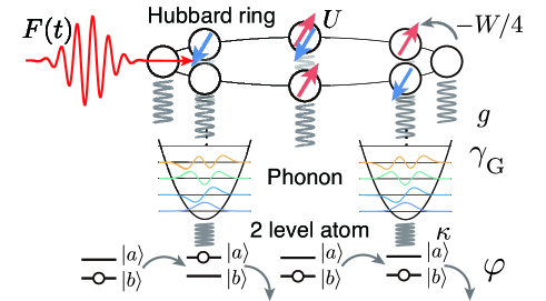
Figure 1: (color online): Schematic description of our hamiltonian. A Hubbard ring $\hat{H}_{\rm H}(t)$ coupled to phonons $\hat{a}_{\pm q_{0}}$ is excited by a time-dependent electric field $F(t)$. These phonons are also coupled to two-level atoms. We additionally introduce phonon dissipation with a phenomenological decay constant $\gamma_{\rm G}$ and with randomizing the phases of wave function $\varphi$ (see Appendix A.1 and A.2 for details).

Our hamiltonian reads

$$\hat{H}(t)=\hat{H}_{\rm H}(t)+\hat{H}_{b}+\hat{H}_{\rm fb}+\hat{H}_{\rm JC},$$ (1)

which is schematically illustrated in Fig. 1. A Hubbard ring under a time-dependent electric field $dF(t)/dt$ is defined as

$$\hat{H}_{\rm H}(t)=-\frac{W}{4}\sum_{i,\sigma}\left[e^{iF(t)}\hat{c}^{\dagger}_{i+1\sigma}\hat{c}^{\ }_{i\sigma}+{\rm h.c.}\right]+U\sum_{i}\hat{n}^{\ }_{i\uparrow}\hat{n}^{\ }_{i\downarrow},$$ (2)

where, $W$ is the band width, $\hat{c}^{\dagger}_{i\sigma}$ ($\hat{c}^{\ }_{i\sigma}$) is the operator creating (destroying) an electron with $\sigma$-spin at the $i$-th site, and $U$ is the on-site Coulomb repulsion. Here the electron number operators are defined as $\hat{n}^{\ }_{i\sigma}=\hat{c}^{\dagger}_{i\sigma}\hat{c}^{\ }_{i\sigma}$.

We introduce bosons that exchange energy and momentum to realize the energy, and momentum relaxations, which are subtantiated by (acoustic) phonons in real solids. Two modes of bosons (denoted by $\nu$ and $\mu$) are introduced by the Hamiltonian $\hat{H}_{\rm b}$ described by

$$\hat{H}_{\rm b} = \hbar\omega_{\rm b}\sum_{u=\nu,\mu}\left(\hat{a}^{\dagger}_{u}\hat{a}^{\ }_{u}+\frac{1}{2}\right),$$ (3)

where $\hat{a}^{\dagger}_{u}$ ($\hat{a}^{\ }_{u}$) is the creation (annihilation) operator of a boson mode with the label $u=\nu,\mu$ with energy $\hbar\omega_{\rm b}$. Here $\nu=q_{0}$ and $\mu=-q_{0}$ specify momenta $\pm q_{0}=\pm 2\pi/L$, where $L$ is the number of sites. The coupling of the bosons to the electrons are described by $\hat{H}_{\rm fb}$:

$$\hat{H}_{\rm fb} = g\sum_{k=2\pi\ell/L}\left[\hat{c}^{\dagger}_{k}\hat{c}^{\ }_{k+q_{0}}\left(\hat{a}^{\ }_{\mu}+\hat{a}^{\dagger}_{\nu}\right)+{\rm h.c.}\right],$$ (4)

where $g$ is the coupling constant. These bosons change the total momentum of the electron wave function with minimal increment and decrement in momenta for the $L$-site Hubbard ring. We also introduce a 2-level atom coupled to each mode of the boson. These atoms absorb and supply the bosons. The coupling between the two 2-level atoms (labeled by $\alpha$ and $\beta$) and bosons is described by $\hat{H}_{\rm JC}$ [14, 15] as

$$\hat{H}_{\rm JC}=\frac{\hbar\omega_{\rm b}}{2}(\sigma_{z}^{(\alpha)}+\sigma_{z}^{(\beta)})+\hbar\kappa\sum_{u=\nu,\mu}(\hat{a}^{\dagger}_{u}\sigma_{-}^{(\alpha)}+\hat{a}^{\ }_{u}\sigma_{+}^{(\alpha)}),$$ (5)

where $\sigma^{(\alpha/\beta)}_{z}$ is a diagonal Pauli matrix and $\sigma^{(\alpha/\beta)}_{\pm}$ are ladder operators interchanging the eigenstates of $\sigma^{(\alpha/\beta)}_{z}$. $\hbar\kappa$ is the coupling constant between the 2-level atoms and bosons. Here the energy difference of the levels between the ground state and the excited state of the atom, denoted by $|b\rangle$ and $|a\rangle$, respectively, is chosen as the energy of the boson mode $\hbar\omega_{\rm b}$.

By employing the time-dependent hamiltonian $\hat{H}(t)$, the photo-excitation and relaxation processes of the correlated electron systems will be studied in the following part of the present paper. Before going into details, we remark the generality of the present one-dimensional model as a prototype of strongly correlated electron systems including those in higher dimensional systems. One may suspect that the Tomonaga-Luttinger liquid behaviors may govern dynamical processes of the one-dimensional Hubbard ring which should be in a strict sense distinct from the universal Landau’s Fermi liquid behaviors in higher dimensional correlated metals. However, finite-size systems with finite time span and finite energy resolution in the present study do not distinguish the Tomonaga-Luttinger liquid behaviors from those of the Fermi liquid and do not hamper us from extracting general tendency of the dynamical processes in the correlated electron systems.

The relaxation of the dark-side spectra is proposed to be dominated by the relaxation of simple particle-hole excitations. The particle-hole excitations in the one-dimensional electron systems hardly remain as well-defined qausiparticles under the presence of the electron-electron interactions: The particle-hole excitations in one-dimensional interacting electron systems, for example, described by the Hubbard ring are reconstructed into collective excitations orthogonal to fermionic excitations in the thermodynamic limit, which is characterized by the Tomonaga-Luttinger liquid behaviors. However, the quasiparticle residue $Z$ remains finite even in the one-dimensional systems provided that the Hubbard ring with finite sites are examined: The quasiparticle residue $Z$ in the one-dimensional interacting electron systems is scaled by the power of the system size although $Z$ approaches zero as the system size increases[16]. Therefore, even though the one-dimensional Hubbard ring is employed, the relaxation processes in the numerical simulation given in the following sections are not specific to the one-dimensional systems except the relatively slow spin relaxations nearly decoupled from the charge excitations.

2.2 Method for time evolution

The wave function of the Hubbard ring coupled to the bath can be expanded by using the basis representing the $N$-electron eigenstates of the Hubbard ring $|\Phi_{m}^{(N)}\rangle$, the Fock states of the phonons $|n_{\nu}\rangle$ and $|n_{\mu}\rangle$, where $n_{\nu}$ and $n_{\mu}$ are numbers of phonons in the each modes, and the eigenstates of the two-level atoms $|\alpha\rangle$ and $|\beta\rangle$, as given as,

$$|\Phi(t)\rangle=\sum_{m=1}^{N_{\rm dim}}\sum_{n_{\nu}=0}^{L_{\rm B}-1}\sum_{n_{\mu}=0}^{L_{\rm B}-1}\sum_{\alpha=a,b}\sum_{\beta=a,b}C_{m;n_{\nu},n_{\mu};\alpha,\beta}(t)$$

$$\times|\Phi_{m}^{(N)}\rangle\otimes|n_{\nu}\rangle\otimes|n_{\mu}\rangle\otimes|\alpha\rangle\otimes|\beta\rangle.$$ (6)

As detailed below, the time-evolution based on the wave function is twofold. Together with the ordinary time-ordered hamiltonian dynamics

$$|\Phi(t)\rangle=T\exp\left[-i\int_{t_{0}}^{t}dt\hat{H}(t)\right]|\Phi(t_{0})\rangle,$$ (7)

started with the ground state wavefunction $|\Phi(t_{0})\rangle$, energy, momentum and phase relaxations of the total system are phenomenologically achieved through the stochastic surrogate hamiltonian approach [17] and a damping constant $\gamma_{\rm G}$ of the boson numbers [18], as detailed in Appendix A and B. The former realizes repeating and successive decoupling of the 2-level atoms from the bosons, and reset of the 2-level atoms to their ground states accompanied by randomization of their phases, everytime after a fixed interval of the time evolution by the Hamiltonan $\hat{H}$.

We use a specific form of $F(t)$,

$$F(t)=\int_{t_{0}}^{t}dt^{\prime}A_{0}e^{-(t^{\prime}-t_{0})^{2}/t_{d}^{2}}\cos\left[\omega_{\rm pulse}(t^{\prime}-t_{0})\right],$$ (8)

to represent applied pulsed lasers with the amplitude $A_{0}$, the pulse center $t_{0}$, the pulse width $t_{d}$, and the frequency $\omega_{\rm pulse}$.

2.3 Spectral functions

We calculate the momentum $k$ and frequency $\omega$ dependent spectral weight $A(k,\omega;t)$ and its occupied part $A_{\rm occ}(k,\omega;t)$ from the time evolution, by projecting the bosons and the two-level atoms out and by taking a long-time approximation that we call stretched-time Lehmann-representation methods. The stretched-time Lehmann representation is nothing but a Lehmann representation based on a projected electronic wave function $|\Phi(t)\rangle_{\rm proj}$ as detailed in Appendix C. The projected wave function is prepared by operating a projection operator

$$\hat{P}_{0} = (\sum_{m}|\Phi_{m}^{(N)}\rangle\langle\Phi_{m}^{(N)}|)$$ (9)

$$\otimes \langle n_{\nu}{\rm=0}|\otimes\langle n_{\mu}{\rm=0}|\otimes\langle{\rm\alpha={\it b}}|\otimes\langle{\rm\beta={\it b}}|,$$

to the wave function $|\Phi(t)\rangle$ as

$$|\Phi(t)\rangle_{\rm proj}=\hat{P}_{0}|\Phi(t)\rangle=\sum_{m=1}^{N_{\rm dim}}a_{m}(t)|\Phi_{m}^{(N)}\rangle,$$ (10)

where $a_{m}(t)=C_{m;0,0;b,b}(t)$.

This method enables the frequency representation of transient phenomena although it satisfies Freericks-Krishnamurthy-Pruschke’s resolution limit only approximately because of the finite probe-pulse width [3]. Typically $\mathcal{O}(10^{2})$ fs pulses give us the spectrum resolution $\sim$ $\mathcal{O}(10^{-2})$ eV, which justifies our results given below.

2.4 Effective temperatures

Here we show how to estimate the effective temperatures of the physical quantities. Our estimation is based on results of the angle-integrated spectra,

$$A_{\rm occ}(\omega,t)=\sum_{k}A_{\rm occ}(k,\omega;t),$$ (11)

and

$$A(\omega,t)=\sum_{k}A(k,\omega;t).$$ (12)

The distribution function is defined as

$$n(\omega,t)=A_{\rm occ}(\omega,t)/A(\omega,t),$$ (13)

which corresponds to the Fermi-Dirac distribution if an effective temperature becomes well-defined.

When we fit the time-dependent spectra by an exact electronic spectra at a finite temperature $T_{\rm eff}$, we can estimate effective temperatures from two different functions, namely, the temperature of $n(\omega,t)$ and that of $A(\omega,t)$. Here, we introduce the exact electronic (occupied) spectra at finite temperatures $A^{\rm(e)}(\omega,k_{\rm B}T_{\rm eff})$ and the distribution functions $n^{\rm(e)}(\omega,k_{\rm B}T_{\rm eff})$. Then we can estimate the temperatures estimated from the following function by minimizing

$$\chi^{2}[f^{\rm(e)},f](t;{T_{\rm eff}})=\int_{\Lambda_{1}}^{\Lambda_{2}}d\omega\left|f^{({\rm e})}(\omega,k_{\rm B}{T_{\rm eff}})-f(\omega,t)\right|^{2}.$$

The effective temperature $T_{\rm eff}$ that minimizes

$$\chi^{2}_{n}(t;T_{\rm eff})\equiv\chi^{2}[n^{\rm(e)},n](t;T_{\rm eff}),$$ (15)

and

$$\chi^{2}_{A}(t;T_{\rm eff})\equiv\chi^{2}[A^{\rm(e)},A](t;T_{\rm eff}),$$ (16)

are denoted by ${T_{\rm eff}}_{n}(t)$ and ${T_{\rm eff}}_{A}(t)$, respectively. If the photo-excited states are really described by the thermally excited ones, these two temperatures should be the same, namely, ${T_{\rm eff}}_{n}(t)={T_{\rm eff}}_{A}(t)$.

3 Results

We simulate relaxation of photo-excited strongly correlated metals. The spectra of the strongly correlated metals in equilibrium show a typical structure regardless of dimensionality of the systems: The spectra consist of the incoherent upper Hubbard band located around $\omega\sim U$, the incoherent lower Hubbard band located for $\omega\lesssim 0$, and the low-energy coherent band around the Fermi energy $\mu_{\rm F}$ [19, 20, 21]. While the upper Hubbard continuum is well separated from the low-energy coherent band, the latter and the lower Hubbard band touch each other or are not separable, in general. For the later discussion, we call the unoccupied part of the low-energy excitations including the quasiparticle band as mid-gap states. We especially highlight relaxations of dark side mid-gap states of doped Mott insulators after photo excitation by a laser pulse.

Below, we set the energy unit $W/4=\hbar=1$. Parameters used for real-time evolutions are $N_{\uparrow}=N_{\downarrow}=3$, $L=8$, $U=8$, $\omega_{\rm b}=\sqrt{2}/4$, $g=0.05$, $\lambda=\tan^{-1}19\pi/40\sim 0.08$, and $\gamma_{\rm G}\Delta t=0.05$ with a time interval $\Delta t=0.1$. We use pulses with frequencies $\omega_{\rm pulse}=\sqrt{2}/4$ much lower than direct gaps between occupied states and upper Hubbard bands. Typically, laser pulses used in this paper give energy $\sim 0.01$ mJ/cm² to electrons if we set $W/4=0.5$ eV and the inter-site distance as 3 Å. The unit time of the present system corresponds to $\sim$ 1.32 fs.

Here we use pulses with frequencies $\omega_{\rm pulse}$ much lower than direct gaps between occupied states and upper Hubbard bands. Even though the photon energy is not enough for direct transitions to the upper Hubbard band, both of the mid-gap low-energy states just above the Fermi level and the upper Hubbard bands are excited due to the short width of pulses and the energy-time uncertainty relation.

3.1 Relaxation of mid-gap states, upper Hubbard bands, and effective temperatures

First, we show relaxation of the density of states in Fig.2. A pulsed laser with duration $t_{d}=5$ and amplitude $A_{0}=4$ excites the system and induces nonequilibrium mid-gap excited states within an energy window, $\mu_{\rm F}\simeq 0.85<\omega\lesssim E_{\rm UHB}=4$, and upper Hubbard bands ($E_{\rm UHB}=4\lesssim\omega$), where $\mu_{\rm F}$ is the Fermi energy. Here, $E_{\rm UHB}$ is chosen as an upper bound of the low-energy spectrum around the Fermi energy $\mu_{\rm F}$.

We observe that the upper Hubbard band relaxes first. The mid-gap states absorb the relaxed excitations from the upper Hubbard band and it joins in the relaxation.

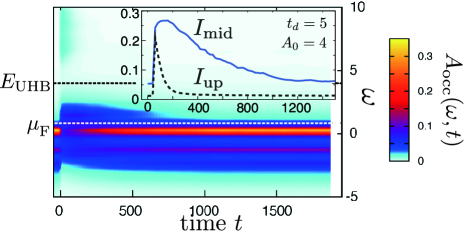
Figure 2: (color online): Relaxation of occupied density of states for $U/t=8$ with 6 electrons ($N_{\uparrow}=N_{\downarrow}$) on a 8-site ring. A laser pulse with $t_{d}=5$, $A_{0}=4$, and $\omega_{\rm pulse}=\sqrt{2}/4$ is used. The center of the pulse is located at $t=0$. Inset shows time-dependence of integrated spectral weights for mid-gap states and upper Hubbard bands, $I_{\rm mid}$ and $I_{\rm up}$. A finite line width $\delta=0.2$ is used for the spectra.

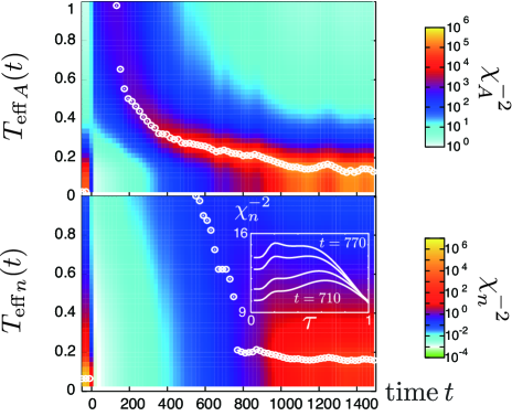
Figure 3: (color online): Time-dependent effective temperatures of distribution functions ${T_{\rm eff}}_{n}(t)$ and spectral functions ${T_{\rm eff}}_{A}(t)$ are shown by white circles with $\chi^{-2}_{n}$ and $\chi^{-2}_{A}$ in color plots. Inset shows double peak structures of $\chi^{-2}_{n}(t;T_{\rm eff})$ around $t=740$, which induce abrupt changes in ${T_{\rm eff}}_{n}(t)$.

By using the following integrated spectral weights,

$$I_{E_{1};E_{2}}(t)=\int_{E_{1}}^{E_{2}}d\omega A_{\rm occ}(\omega,t)/\int_{-\infty}^{+\infty}d\omega A_{\rm occ}(\omega,t),$$ (17)

we here define the integrated spectral weights for the mid-gap states and upper Hubbard bands as $I_{\rm mid}(t)=I_{\mu_{\rm F};E_{\rm UHB}}(t)$ and $I_{\rm up}(t)=I_{E_{\rm UHB};+\infty}(t)$, respectively. The integrated spectral weights $I_{\rm mid}$ and $I_{\rm up}$ are summarized in the inset of Fig. 2. The relaxation rate of $I_{\rm mid}$ up to $t\sim 10^{3}$ depends on the square of $g$ when other parameters are fixed, while the relaxation at longer time scales is additionally affected by phase relaxation. We employ $g$ to reproduce the experimental relaxation rate of doped Mott insulators [5, 22, 23, 24] in the time range up to $t\sim 10^{3}$, irrespective of ultrashort-time relaxation mechanisms that may depend on dimensionality and details of the hamiltonian [25, 26, 27].

The numerical results of the effective temperatures ${T_{\rm eff}}_{n}(t)$ and ${T_{\rm eff}}_{A}(t)$ are shown in Fig.3, where the energy windows are chosen to extract low-energy contribution as $\Lambda_{1}=-3$ and $\Lambda_{2}=+3$ ($\Lambda_{1}=-\infty$ and $\Lambda_{2}=E_{\rm UHB}$) are set for $T_{{\rm eff}n}(t)$ ($T_{{\rm eff}A}(t)$) in Eq.(2.4). Around the occupied band bottom and the upper Hubbard band distant from the Fermi energy $\mu_{\rm F}$, the density of states in non-equilibrium tends to deviate from the counterpart in equilibrium more significantly than the density of states around the Fermi energy $\mu_{\rm F}$ (for example, see Fig.1 of Ref.Ohnishi15).

The effective temperatures ${T_{\rm eff}}_{n}(t)$ and ${T_{\rm eff}}_{A}(t)$ are significantly different as shown in Fig.3, which clearly demonstrates that the spectral weights relaxes faster than the distribution functions. The deformation of the spectral weights is nothing but a manifestation of the electron correlations, which invalidates simple effective electron temperature approaches. The deformation of the spectral weights also means that the excited carriers above the Fermi level are not injected to the dark-side of the equilibrium spectra, in contrast to a naive expectation for visualizing the dark-side with hot carriers.

In contrast to the relaxation of the spectral function, the relaxation of the distribution function is not smooth as shown in the time dependence of ${T_{\rm eff}}_{n}(t)$ (see Fig.3). The abrupt change in the time dependence of ${T_{\rm eff}}_{n}(t)$ is a manifestation of a strong deviation from the equilibrium high-temperature distribution for a short time after the irradiation, $t\lesssim 800$. Similar strong deviations from the equilibrium distribution in initial stages of hot carrier relaxation are reported for phonon-assisted relaxation of hot carriers in free electron systems [28].

3.2 Angle-resolved and unoccupied spectra through logarithmic differences in relaxation processes

Next, we examine momentum-resolved nonequilibrium spectra. In Fig. 4(a), we show the equilibrium momentum-resolved spectrum with the same parameter set used in Fig. 2 and 3. Just after the photo-excitation, the occupied spectrum $A_{\rm occ}(k,w;t)$ becomes completely different from the spectrum in equilibrium shown in Fig. 4(a). As evident in Fig. 4(b), the peaks in nonequilibrium spectra are not coincident with the peaks in equilibrium unoccupied states.

Therefore, to observe or estimate the dark-side equilibrium spectra of doped Mott insulators, photo-excited electrons are seemingly useless. However, after closer inspection, we realize that, from the photo-excited spectra, the dark-side equilibrium spectra can be estimated as proposed below.

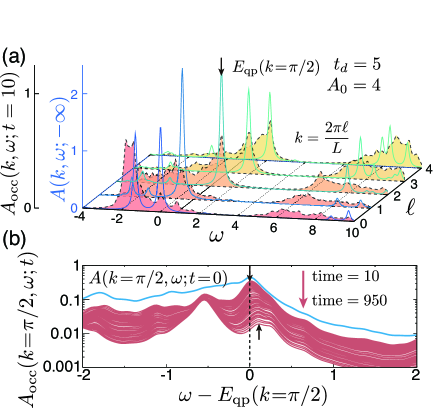
Figure 4: (color online): (a) Spectrum of a doped Mott insulator out of equilibrium, $A_{\rm occ}(k,\omega;t)$ in comparison with total spectrum in equilibrium $A(k,\omega;-\infty)$. The shaded area shows occupied spectrum $A_{\rm occ}(k,\omega;t)$ and the solid curves show total spectrum $A(k,\omega;-\infty)$ in equilibrium. The shaded area appears at energy ranges where no equilibrium unoccupied states exist. (b) Time-dependent spectra at smallest unoccupied momentum $k=\pi/2$ from $t=10$ to $t=950$. The nonequilibrium spectra have a prominent peak at the equilibrium quasiparticle peak $\omega=E_{\rm qp}(k=\pi/2)$ (downward arrow) , while they have peaks at $\omega$ different from the energy of the equilibrium peak as well, as indicated by the upward vertical arrow. A finite line width $\delta=0.2$ is used as in Fig.2.

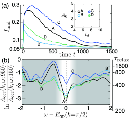
Figure 5: (color online): (a) Time-dependences of mid-gap weights $I_{\rm mid}$. The partial swap introduces noise in $I_{\rm mid}$. Inset shows parameter sets of $t_{d}$ and $A_{0}$. The circle A corresponds to the parameter set $t_{d}=5$ and $A_{0}=4$ used in Fig. 2 and 3. (b) Logarithmic differences and $\tau_{\rm relax}$ in nonequilibrium occupied spectra at the smallest unoccupied momentum $k=\pi/2$. When laser pulses with $A_{0}>3$ are used, the logarithmic differences show significant minima.

Here, we propose an approach to extract the dark-side spectra in equilibrium, which may replace the standard effective temperature approach. We focus on energy- and momentum-resolved relaxation rates of $A_{occ}(k,\omega;t)$ and frame a hypothesis: The relaxation rates of excited nonequilibrium states have local maxima when the states are located at the unoccupied quasiparticle energy in equilibrium. The hypothesis seemingly contradicts Landau’s Fermi liquid theory [29], in which the quasiparticles’ life times are longer than incoherent states in equilibrium. However, outside the equilibrium, the quasiparticle excitations have efficient relaxation pathways as detailed below.

Then, we explain how the photo-excited states in the dark side consisting the quasiparticles relax faster than the incoherent excitations. First of all, we assume correspondence of a many-body excited state with small total momentum $|q_{0}|$ to unoccupied quasiparticle peak due to added electrons in equilibrium, which is a central notion of the Fermi liquid theory. In equilibrium, the detailed balance between emission and absorption of the phonons and the Pauli blocking guarantee long life times of quasiparticles even in the presence of the electron-phonon couplings [30]. However, out of equilibrium, where the detailed balance and the Pauli blocking become inefficient, single particle-hole excitation easily decays by emitting energy and momentum through the electron-phonon couplings. Due to the short-time violation of the energy conservation, the particle-hole excitations decay through first order perturbation process of the electron-phonon coupling $g$. Therefore, by recalling the first assumption, out-of-equilibrium states injected at the quasiparticle peaks decay faster than more complicated excited states such as multiple particle-hole excitations.

To extract spectral components with large relaxation rates, we propose and use logarithmic differences of nonequilibrium occupied spectra $A_{\rm occ}(k,\omega;t)$ for some time interval from $t_{1}$ until $t_{2}$, which gives an averaged relaxation time $\tau_{\rm relax}(k,\omega)$ as

$$\frac{-1}{{\color[rgb]{0,0,0}\tau_{\rm relax}(k,\omega)}}\sim{\color[rgb]{0,0,0}\frac{1}{t_{2}-t_{1}}}\ln\frac{A_{\rm occ}(k,\omega;t_{2})}{A_{\rm occ}(k,\omega;t_{1})}.$$ (18)

By this average, the effects of unavoidable noise in experiments are suppressed. The slow relaxation of $I_{\rm mid}$ in comparison with the probe laser pulse width ($\sim$ 100 fs) validates our stretched-time Lehmann representation, where $t_{2}-t_{1}$ $(>0)$ longer than the relaxation time of $I_{\rm mid}$ is also better.

In Fig. 5, we show the usefulness of the logarithmic differences of the nonequilibrium unoccupied spectra. For sufficiently large amplitude of laser pulses, we obtain significant minima of the logarithmic differences as functions of $\omega$. The minima agree with the quasiparticle peak, as illustrated in Fig. 5(b). In contrast, for smaller amplitude of laser pulses, the minima become less significant and are not coincident with the quasiparticle peak as shown in Fig.7 of Appendix D.

It is crucial to use the laser-pulse amplitude $A_{0}$ in an appropriate range. The laser pulse must generate particle-hole excitations efficiently beyond the linear-response regime in a controlled way, which requires $A_{0}$ to be comparable with that required for the Bloch oscillation, $A_{\rm Bloch}$. We propose to choose $A_{0}$ in an extended range roughly given by $A_{0}>\omega_{\rm pulsse}>1/t_{d}$ but not $A_{0}\gg 1/t_{d}$. See the detailed condition for the pump laser in the Appendix D.

4 Summary and Discussion

In this paper, we have simulated relaxation of photo-excited doped Mott insulators by employing a Hubbard ring coupled with bosonic degrees of freedom. We have shown the existence of two distinct effective electronic temperatures that make the standard effective-temperature approaches unjustified. We instead propose a method to extract the dark-side equilibrium spectra from nonequilibrium pump-probe relaxation by using logarithmic difference of the time-dependent spectra. The logarithmic difference offers a stable experimental tool that circumvents inevitable noises in the experiments.

We have also explored sufficient conditions for detectable signals in experiments: Amplitude of the pumping laser is required to satisfy $A_{0}>\omega_{\rm pulse}>1/t_{d}$. The laser pulses with a sufficiently large amplitude generates photo-excited states consisting of combinations of elementary excitations and quasiparticle excitations. It enables us to extract the equilibrium dark-side spectra from the photo-excited nonequilibrium spectra.

The elementary excitations in equilibrium have relatively fast relaxation paths in the photo-excited nonequilibrium states. The proposed method opens a novel way to access the momentum-resolved dark-side spectra of the strongly correlated electron systems.

The newly proposed scheme to access the dark-side spectra will be helpful for the studies on unoccupied spectra of high-$T_{\rm c}$ superconducting cuprates [11]. It gives us a direct access to structure and formation of the so-called pseudogap in the cuprate superconductors, which hold a key for understanding the mechanism of the high-temperature superconductivities in the cuprates.

The authors thank Kyoko Ishizaka for fruitful discussion about pump-probe measurements. Y.Y. thank Takashi Oka and Yasuhiro Yamada for their comments on the present work. We acknowledge the financial supports by a Grant-in-Aid for Scientific Research (No. 22104010 and No. 22340090) from MEXT, Japan, and a Grant-in-Aid for Scientific Research on Innovative Areas ‘Materials Design through Computics: Complex Correlation and Non-Equilibrium Dynamics.’ This work was also supported by MEXT HPCI Strategic Programs for Innovative Research (SPIRE) (under the grant number hp130007 and hp140215) and Computational Materials Science Initiative (CMSI).

In this Appendix, we detail the simulation method for the energy, momentum and phase realized by the surrogated hamiltonian [17]. The stretched-time Lehmann-representation methods are also introduced. Constraint on pulse laser for efficient observation of quasiparticle excitations is also detailed.

Appendix A Energy, momentum, and phase relaxation

A.1 Swapping operator

As expalined in the main article, we introduce an operator, namely, swapping operator that stands for the reset of the 2-level atoms to its ground states $|b\rangle$ and replacing the phases of the electronic and bosonic wave functions with random phases with the periodic time interval $\Delta t$. Our swapping operator is defined as

$$\hat{O}_{\rm swap}|\Phi(t)\rangle=\sum_{m=1}^{N_{\rm dim}}\sum_{n_{\nu}=0}^{L_{\rm B}-1}\sum_{n_{\mu}=0}^{L_{\rm B}-1}\sqrt{\sum_{\alpha,\beta=a,b}\left|C_{m;n_{\nu},n_{\mu};\alpha,\beta}(t)\right|^{2}}$$

$$\times e^{i\varphi_{m;n_{\nu},n_{\mu}}}|\Phi_{m}^{(N)}\rangle\otimes|n_{\nu}\rangle\otimes|n_{\mu}\rangle\otimes|b\rangle\otimes|b\rangle,$$ (19)

where $\varphi_{m;n_{\nu},n_{\mu}}$ is a random phase.

We also use a partial swap defined by the following partial swapping operator:

$$\hat{O}_{\rm pswap}=\hat{1}+\lambda\hat{O}_{\rm swap},$$ (20)

where $\hat{1}$ is an identity operator. After applying the $\hat{O}_{\rm swap}$ and $\hat{O}_{\rm pswap}$, we normalize the wave function.

A.2 Additional disspation mechanism

To control the temperatures of the lattice, which is mimicked by the two boson modes, in addition to the swapping operators, we use a Landau-Lifshitz and Gilbert-type dissipation operator to keep the number of bosons small enough partially following Gisin’s idea (see Ref.Gisin) for the time interval $\Delta t$:

$$\hat{O}_{\rm Gisin}|\Phi(t)\rangle=\sum_{m=1}^{N_{\rm dim}}\sum_{n_{\nu}=0}^{L_{\rm B}-1}\sum_{n_{\mu}=0}^{L_{\rm B}-1}\sum_{\alpha=a,b}\sum_{\beta=a,b}C_{m;n_{\nu},n_{\mu};\alpha,\beta}(t)$$

$$\times e^{-\gamma_{\rm G}\Delta t(n_{\nu}+n_{\mu})}|\Phi_{m}^{(N)}\rangle\otimes|n_{\nu}\rangle\otimes|n_{\mu}\rangle\otimes|\alpha\rangle\otimes|\beta\rangle,$$ (21)

where $\gamma_{\rm G}$ is a phenomenological decay constant of the number of the bosons, Here, we impose the condition that the equilibrium temperature to be zero, because experimental temperature is normally negligible in terms of the excited energy of electrons.

For practical numerical treatments, the additional dissipation mechanism with the decay constant $\gamma_{\rm G}$ is helpful since it keeps the averaged bosonic number small and, therefore, reduces the truncation errors for the bosonic Hilbert space. In a real crystalline solids, the number of the phonon modes is large enough to keep the density of the bosons. However, due to the limit of computational resources, we employ a minimal phonon subsystem. Therefore, we need to get rid of excess accumulation of the bosons due to the limited number of the phonon modes. The decay constant $\gamma_{\rm G}$ is again useful to avoid the accumulation of the bosons.

Appendix B Time evolution

Our time evolution consists of 2 steps as detailed below: First, we calculate the hamiltonian time-evolution as

$$|\widetilde{\Phi}(t_{i+1})\rangle=T\exp\left[-i\int_{t_{i}}^{t_{i+1}}dt\hat{H}(t)\right]|\Phi(t_{i})\rangle,$$ (22)

where $Te^{-i\int_{t_{i}}^{t_{i+1}}\hat{H}(t)}$ is a time-ordered operator. Next, we apply the swapping operator,

$$|\Phi(t_{i+1})\rangle=\frac{\hat{O}_{\rm pswap}\hat{O}_{\rm Gisin}^{{\color[rgb]{0,0,0}M}}|\widetilde{\Phi}(t_{i+1})\rangle}{\sqrt{\left|\hat{O}_{\rm pswap}\hat{O}_{\rm Gisin}^{{\color[rgb]{0,0,0}M}}|\widetilde{\Phi}(t_{i+1})\rangle\right|^{2}}}.$$ (23)

We successively repeat the above 2 steps. The swapping time defined by $t_{\rm swap}=t_{i+1}-t_{i}$ $(={\color[rgb]{0,0,0}M}\Delta t)$ controls the phase relaxation, and an energy relaxation as well. In this study, we set $M=200$.

Appendix C Ansatz for spectrum

Here we introduce an approximate method to calculate time-dependent spectral functions. The spectral functions revealed by time-dependent angle-resolved photoemission spectra provide us with physical pictures. The present formalism corresponds to the limit of the long-time window of the laser pulse used as the probe (see Ref.Freericks). We call the following approximate method as stretched-time Lehmann spectral representation.

C.1 Projection

First, we need to eliminate the bosonic degrees of freedom and project the entire wave function onto the $N$-electron partial Hilbert space expanded by $\{|\Phi_{m}^{(N)}\rangle\}$ as in Eq.(10):

$$|\Phi(t)\rangle_{\rm proj}=\sum_{m=1}^{N_{\rm dim}}a_{m}(t)|\Phi_{m}^{(N)}\rangle.$$ (24)

Here, we expand the projected wave function by the $N$-particle eigenstates of $\hat{H}_{\rm H}(t=0)$, $\{|\Phi_{m}^{(N)}\rangle\}$.

C.2 Ansatz

As an important observable in experiments, the time-dependent spectral functions have often been discussed. However, the energy-resolved spectral functions are definitely approximate ones whenever the observations are carried out in non-steady states (see Ref.Freericks). If the time-dependence of the system is slow enough in comparison with the time scale set by resolution limits, the approximate time-dependence of the energy-resolved spectral functions becomes well-defined. Here we apply the following ansatz justified in the steady-state limit: Starting from $|\Phi(t)\rangle_{\rm proj}$, we define an approximate time-dependent Green’s function for the occupied and unoccupied states as,

$$G_{\rm occ}(k,\omega;t)=\sum_{n,m}|a_{m}(t)|^{2}$$

$$\times\frac{\langle\Phi^{(N)}_{m}|\hat{c}^{\dagger}_{k\sigma}|\Phi^{(N-1)}_{n}\rangle\langle\Phi^{(N-1)}_{n}|\hat{c}^{\ }_{k\sigma}|\Phi^{(N)}_{m}\rangle}{\omega+i\delta+E_{n}^{(N-1)}-E_{m}^{(N)}},$$ (25)

and

$$G_{\rm uno}(k,\omega;t)=\sum_{n,m}|a_{m}(t)|^{2}$$

$$\times\frac{\langle\Phi^{(N)}_{m}|\hat{c}^{\ }_{k\sigma}|\Phi^{(N+1)}_{n}\rangle\langle\Phi^{(N+1)}_{n}|\hat{c}^{\dagger}_{k\sigma}|\Phi^{(N)}_{m}\rangle}{\omega+i\delta-E_{n}^{(N+1)}+E_{m}^{(N)}},$$ (26)

where $E_{m}^{(N)}$ is the eigenvalue that corresponds to $|\Phi_{m}^{(N)}\rangle$.

By using the above ansatz for the Green’s functions, we can define the stretched-time Lehmann spectral representation as

$$A(k,\omega;t)=-\frac{1}{\pi}{\rm Im}\left[G_{\rm occ}(k,\omega;t)+G_{\rm uno}(k,\omega;t)\right].$$ (27)

Here we note that the occupied spectrum is given by an occupied Green’s function defined as

$$A_{\rm occ}(k,\omega;t)=-\frac{1}{\pi}{\rm Im}\left[G_{\rm occ}(k,\omega;t)\right].$$ (28)

Appendix D Pumping laser dependence

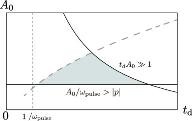
Figure 6: Constraints on amplitude $A_{0}$ and duration $t_{d}$ of laser pulses to observe quasiparticles with momentum amplitude $|p|$. The curves and lines are determined by $A_{0}/\omega_{\rm pulse}=|p|$, $t_{d}A_{0}={\rm const.}$, and $t_{d}=1/\omega_{\rm pulse}$. The dashed curve qualitatively illustrates the upper bound of $A_{0}$, below which the “adiabatic transitions” accompanying the particle-hole excitations efficiently occur by suppressing the Landau-Zener tunneling. The shaded parameter region is suitable for generating a pair of particle-hole excitations.

There is an optimal parameter range of amplitude and duration of laser pulses for efficient observations of the dark-side spectra by utilizing the logarithmic differences of the time-dependent angle-resolved photoemission intensities. For the efficient observation, the laser pulses are required to efficiently generate particle-hole excitations including the desired momentum $p$ intended to measure the quasiparticle. Below, we clarify what are the optimal amplitude and duration of the laser pulses.

We start with two trivial constraints. The efficient observations are hampered in two regions. For $\omega_{\rm pulse}t_{d}\ll 2\pi$, the laser pulse contains less than a single cycle of electric-field oscillations, which is called a subcycle laser pulse. Subcycle laser pulses are expected to generate net electric currents strongly depending on their pulse shape or phase. Thus, the subcycle pulses are not suitable for stable observations of the dark side. The other trivial constraint comes from pump fluence. For too large pump fluence or $t_{d}A_{0}\gg 1$, the system gains too much energy. Then, the relaxation processes involves multiple particle-hole excitations and becomes complicated, which may be observed as sudden increase in relaxation time as laser fluence is increased.

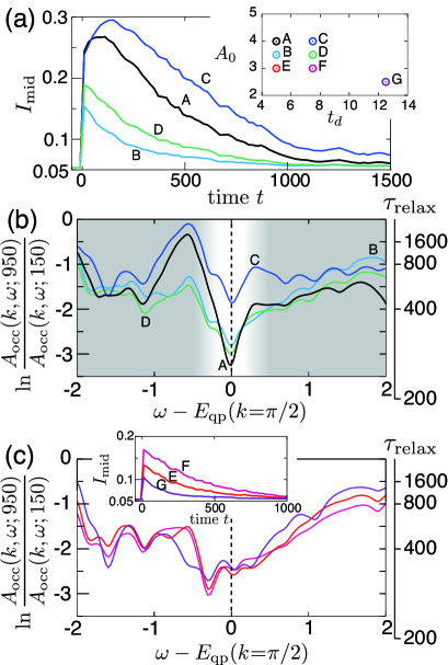
Figure 7: (a) Time-dependences of mid-gap weights $I_{\rm mid}$. The partial swap introduces noise in $I_{\rm mid}$. Inset shows parameter sets of $t_{d}$ and $A_{0}$. (b) Logarithmic differences and $\tau_{\rm relax}$ in nonequilibrium occupied spectra at the smallest unoccupied momentum $k=\pi/2$. When laser pulses with $A_{0}>3$ are used, the logarithmic differences show significant minima. (c) Logarithmic differences and $\tau_{\rm relax}$ at momentum $k=\pi/2$ for $A_{0}\lesssim 3$. The minima are located at $\omega$ different from $E_{\rm qp}$. Inset shows $I_{\rm mid}$ for weakly excited cases with $A_{0}\lesssim 3$.

To gain sufficient intensity of the emitted electrons by the probe laser, the pump light is required to generate sufficient amount of particle-hole excitations. In the present formalism such excitations are generated by the acceleration of electrons by the time dependent vector potential $F(t)/ea$, where $e$ is the elementary charge and $a$ is the lattice constant. The amplitude of the vector potential $F(t)/ea$ is controlled by a parameter $A_{0}$.

Let us clarify how $F(t)\propto A_{0}$ generates the particle-hole excitations. These particle-hole excited states orthogonal to the ground state in the electronic subsystem $\hat{H}_{\rm H}$ are attained by many level crossings generated by the vector potential $F(t)\propto A_{0}$ and additionally by the hybridization gap indirectly induced by the coupling to bosons, which transforms the simple level crossing to the avoided crossing.

When the system originally in the ground state is driven by adiabatically passing through such an avoided crossing, the state becomes containing particle-hole excitations originally orthogonal to the ground state in the absence of the light and bosons. Namely, the particle-hole excitations are generated by the “adiabatic transitions” in the driven system. When the time dependent vector potential $F(t)\propto A_{0}$ is an oscillating pulse with a frequency $\omega_{\rm pulse}$ and a gaussian envelop $\exp\left[-(t-t_{0})^{2}/t_{d}^{2}\right]$, $\omega_{\rm pulse}t_{d}$ determines the number of times that the system passes through the avoided crossing, where $t_{0}$ is the gaussian pulse center in the time domain and $t_{d}$ is the pulse width. Therefore, to increase the chance of such “adiabatic transitions” to particle-hole excited states, we need to drive the system for sufficiently long time $t_{d}$ at least to satisfy $\omega_{\rm pulse}t_{d}\gtrsim 1$ provided that the above condition $t_{d}A_{0}\lesssim 1$ is satisfied.

An additional requirement for the “adiabatic transitions” to occur effectively exists: If $A_{0}$ becomes high, the probability of the non-adiabatic Landau-Zener tunneling at the avoided level crossings increases without following the adiabatic route. It prevents effective generation of particle-hole pairs. Therefore, for higher $A_{0}$, $t_{d}$ is required to be longer to achieve the same density of particle-hole excitations.

Equivalently, an appropriate density of particle-hole excitations are obtained in the region $(1-P_{\rm LZ}(A_{0}))\omega_{\rm pulse}\sim 1/t_{d}$, where the Landau-Zener tunneling probability $0<P_{\rm LZ}<1$ (the probability per each crossing through the avoided energy crossing point) depends on $A_{0}$ and largely increases with $A_{0}$. Thus the “adiabatic transition” with the probability $1-P_{\rm LZ}(A_{0})$ decreases with increasing $A_{0}$. This means that the upper limit of desired $A_{0}$ increases with $t_{d}$.

We also have a constraint that $A_{0}$ has to be larger than another threshold. By noting that the time-dependent phase $F(t)$ causes lattice-momentum shifts, for observation of quasiparticles with momentum amplitude $|p|$, we need the maximum of the time-dependent phase $F(t)$ larger than $|p|$. For a gaussian pulse, the maximum of the phase $F(t)$ is approximately given by $A_{0}/\omega_{\rm pulse}$. Therefore, when we observe the quasiparticles with momentum amplitude $|p|$, we need $A_{0}$ that satisfies $A_{0}/\omega_{\rm pulse}>|p|$. In general, $A_{0}$ required by the above constraint is comparable with that required for the Bloch oscillation, $A_{\rm Bloch}$.

By taking the above constraints into account, the suitable parameter region of the pulse laser amplitude $A_{0}$ and duration $t_{d}$ is determined for the efficient observation of the dark side. The constraints and the obtained parameter region are summarized in Fig.6. The appropriate region for the parameter values is roughly given by $A_{0}>\omega_{\rm pulse}|p|\sim\omega_{\rm pulse}\gtrsim 1/t_{d}$. The parameter values studied in the main text, namely, $A_{0}=4,t_{d}=5$, $\omega_{\rm pulse}=\sqrt{2}/4$, and $|p|=2\pi/L\sim 0.8$ satisfies this criteria.

To demonstrate the general validity of the hypothesis on the relaxation rates in the logarithmic differences, we choose several sets of parameters $t_{d}$ and $A_{0}$, in addition to Fig.5 of the present paper, and show that the hypothesis works if the amplitude of the laser pulse is large enough, here $A_{0}\gtrsim 3$, as illustrated in Fig.7.

References

- [1] U. Bovensiepen, J. Phys.: Condens. Matter 19, 083201 (2007).
- [2] A. Damascelli, Z. Hussain, Z.-X. Shen, Rev. Mod. Phys. 75, 473 (2003).
- [3] J. K. Freericks, H. R. Krishnamurthy, and Th. Pruschke, Phys. Rev. Lett. 102, 136401 (2009).
- [4] P .B. Allen, Phys. Rev. Lett. 59, 1460 (1987).
- [5] L. Perfetti, P. A. Loukakos, M. Lisowski, U. Bovensiepen, H. Eisaki, and M. Wolf, Phys. Rev. Lett. 99, 197001 (2007).
- [6] L. Perfetti, P. A. Loukakos, M. Lisowski, U. Bovensiepen, M. Wolf, H. Berger, S. Biermann, and A. Georges, New J. Phys. 10, 053019 (2008).
- [7] B. Moritz, A. F. Kemper, M. Sentef, T. P. Devereaux, and J. K. Freericks, Phys. Rev. Lett. 111, 077401 (2013).
- [8] S. Hellmann, T. Rohwer, M. Kallne, K. Hanff, C. Sohrt, A. Stange, A. Carr, M. M. Murnane, H. C. Kapteyn, L. Kipp, M. Bauer, and K. Rossnagel, Nature Communications 3, 1069 (2012).
- [9] F. Reinert, D. Ehm, S. Schmidt, G. Nicolay, S. Hüfner, J. Kroha, O. Trovarelli, and C. Geibel, Phys. Rev. Lett. 87, 106401 (2001).
- [10] A. Shimoyamada, S. Tsuda, K. Ishizaka, T. Kiss, T. Shimojima, T. Togashi, S. Watanabe, C. Q. Zhang, C. T. Chen, Y. Matsushita, H. Ueda, Y. Ueda, and S. Shin Phys. Rev. Lett. 96, 026403 (2006).
- [11] S. Sakai, S. Blanc, M. Civelli, Y. Gallais, M. Cazayous, M.-A. Masson, J. S. Wen, Z. J. Xu, G. D. Gu, G. Sangiovanni, Y. Motome, K. Held, A. Sacuto, A. Georges, and M. Imada, Phys. Rev. Lett. 111, 107001 (2013).
- [12] M. Imada, A. Fujimori, and Y. Tokura, Rev. Mod. Phys. 70, 1039 (1998).
- [13] Y. Imry, Introduction to Mesoscopic Physics (Oxford University Press, Oxford, 1997).
- [14] E. T. Jaynes and F. W. Cummings, Proc. IEEE 51, 89 (1963).
- [15] J. H. Eberly, N. B. Narozhny, and J. J. Sanchez-Mondragon, Phys. Rev. Lett. 44, 1323 (1980).
- [16] A. Shashi, M. Panfil, J.-S. Caux, and A. Imambekov, Phys. Rev. B 85, 155136 (2012).
- [17] G. Katz, D. Gelman, M. A. Ratner, and R. Kosloff, J. Chem. Phys. 129, 034108 (2008).
- [18] N. Gisin, J. Phys. A 14, 2259 (1981).
- [19] M. B. J. Meinders, H. Eskes, and G. A. Sawatzky, Phys. Rev. B 48, 3916 (1993).
- [20] D. Sénéchal, D. Perez, and M. Pioro-Ladrière, Phys. Rev. Lett. 84, 522 (2000).
- [21] M. Kohno, Phys. Rev. B 90, 035111 (2014).
- [22] W. Nessler, S. Ogawa, H. Nagano, H. Petek, J. Shimoyama, Y. Nakayama, and K. Kishio, Phys. Rev. Lett. 81, 4480 (1998).
- [23] Y. H. Liu, Y. Toda, K. Shimatake, N. Momono, M. Oda, and M. Ido, Phys. Rev. Lett. 101, 137003 (2008).
- [24] J. D. Rameau, S. Freutel, L. Rettig, I. Avigo, M. Ligges, Y. Yoshida, H. Eisaki, J. Schneeloch, R. D. Zhong, Z. J. Xu, G. D. Gu, P. D. Johnson, and U. Bovensiepen, Phys. Rev. B 89, 115115 (2014).
- [25] H. Okamoto, T. Miyagoe, K. Kobayashi, H. Uemura, H. Nishioka, H. Matsuzaki, A. Sawa, and Y. Tokura, Phys. Rev. B 83, 125102 (2011).
- [26] Z. Lenari and P. Prelovek, Phys. Rev. Lett. 111, 016401 (2013).
- [27] H. Aoki, N. Tsuji, M. Eckstein, M. Kollar, T. Oka, and P. Werner, Prev. Mod. Phys. 86, 779 (2014).
- [28] H. Ohnishi, N. Tomita, and K. Nasu, J. Phys. Soc. Jpn. 84, 043701 (2015).
- [29] A. A. Abrikosov, L. P. Gorkov, and I. E. Dzyaloshinski, Methods of Quantum Field Theory in Statistical Physics (Dover Publications, INC., New York, 1963).
- [30] J. R. Schrieffer, Theory of Superconductivity (Westview Press, Boulder, CO, 1971).